The quasiprobability behind the out-of-time-ordered correlator

Abstract

Two topics, evolving rapidly in separate fields, were combined recently: The out-of-time-ordered correlator (OTOC) signals quantum-information scrambling in many-body systems. The Kirkwood-Dirac (KD) quasiprobability represents operators in quantum optics. The OTOC was shown to equal a moment of a summed quasiprobability [Yunger Halpern, Phys. Rev. A 95, 012120 (2017)]. That quasiprobability, we argue, is an extension of the KD distribution. We explore the quasiprobability’s structure from experimental, numerical, and theoretical perspectives. First, we simplify and analyze the weak-measurement and interference protocols for measuring the OTOC and its quasiprobability. We decrease, exponentially in system size, the number of trials required to infer the OTOC from weak measurements. We also construct a circuit for implementing the weak-measurement scheme. Next, we calculate the quasiprobability (after coarse-graining) numerically and analytically: We simulate a transverse-field Ising model first. Then, we calculate the quasiprobability averaged over random circuits, which model chaotic dynamics. The quasiprobability, we find, distinguishes chaotic from integrable regimes. We observe nonclassical behaviors: The quasiprobability typically has negative components. It becomes nonreal in some regimes. The onset of scrambling breaks a symmetry that bifurcates the quasiprobability, as in classical-chaos pitchforks. Finally, we present mathematical properties. We define an extended KD quasiprobability that generalizes the KD distribution. The quasiprobability obeys a Bayes-type theorem, for example, that exponentially decreases the memory required to calculate weak values, in certain cases. A time-ordered correlator analogous to the OTOC, insensitive to quantum-information scrambling, depends on a quasiprobability closer to a classical probability. This work not only illuminates the OTOC’s underpinnings, but also generalizes quasiprobability theory and motivates immediate-future weak-measurement challenges.

Two topics have been flourishing independently: the out-of-time-ordered correlator (OTOC) and the Kirkwood-Dirac (KD) quasiprobability distribution. The OTOC signals chaos, and the dispersal of information through entanglement, in quantum many-body systems Shenker_Stanford_14_BHs_and_butterfly ; Shenker_Stanford_14_Multiple_shocks ; Shenker_Stanford_15_Stringy ; Roberts_15_Localized_shocks ; Roberts_Stanford_15_Diagnosing ; Maldacena_15_Bound . Quasiprobabilities represent quantum states as phase-space distributions represent statistical-mechanical states Carmichael_02_Statistical . Classical phase-space distributions are restricted to positive values; quasiprobabilities are not. The best-known quasiprobability is the Wigner function. The Wigner function can become negative; the KD quasiprobability, negative and nonreal Kirkwood_33_Quantum ; Dirac_45_On ; Lundeen_11_Direct ; Lundeen_12_Procedure ; Bamber_14_Observing ; Mirhosseini_14_Compressive ; Dressel_15_Weak . Nonclassical values flag contextuality, a resource underlying quantum-computation speedups Spekkens_08_Negativity ; Ferrie_11_Quasi ; Kofman_12_Nonperturbative ; Dressel_14_Understanding ; Howard_14_Contextuality ; Dressel_15_Weak ; Delfosse_15_Wigner . Hence the KD quasiprobability, like the OTOC, reflects nonclassicality.

Yet disparate communities use these tools: The OTOC $F(t)$ features in quantum information theory, high-energy physics, and condensed matter. Contexts include black holes within AdS/CFT duality Shenker_Stanford_14_BHs_and_butterfly ; Maldacena_98_AdSCFT ; Witten_98_AdSCFT ; Gubser_98_AdSCFT , weakly interacting field theories Stanford_15_WeakCouplingChaos ; Patel_16_ChaosCritFS ; Chowdhury_17_ONChaos ; Patel_17_DisorderMetalChaos , spin models Shenker_Stanford_14_BHs_and_butterfly ; HosurYoshida_16_Chaos , and the Sachdev-Ye-Kitaev model Sachdev_93_Gapless ; Kitaev_15_Simple . The KD distribution features in quantum optics. Experimentalists have inferred the quasiprobability from weak measurements of photons Bollen_10_Direct ; Lundeen_11_Direct ; Lundeen_12_Procedure ; Bamber_14_Observing ; Mirhosseini_14_Compressive ; Suzuki_16_Observation ; Piacentini_16_Measuring ; Thekkadath_16_Direct and superconducting qubits White_16_Preserving ; Groen_13_Partial .

The two tools were united in YungerHalpern_17_Jarzynski . The OTOC was shown to equal a moment of a summed quasiprobability, $\tilde{A}_{\rho}$:

$$F(t)=\frac{\partial^{2}}{\partial\beta\,\partial\beta^{\prime}}\left\langle e^{-(\beta W+\beta^{\prime}W^{\prime})}\right\rangle\Bigg{\rvert}_{\beta,\beta^{\prime}=0}\,.$$ (1)

$W$ and $W^{\prime}$ denote measurable random variables analogous to thermodynamic work; and $\beta,\beta^{\prime}\in\mathbb{R}$. The average $\left\langle.\right\rangle$ is with respect to a sum of quasiprobability values $\tilde{A}_{\rho}(.)$. Equation (1) resembles Jarzynski’s Equality, a fluctuation relation in nonequilibrium statistical mechanics Jarzynski_97_Nonequilibrium . Jarzynski cast a useful, difficult-to-measure free-energy difference $\Delta F$ in terms of the characteristic function of a probability. Equation (1) casts the useful, difficult-to-measure OTOC in terms of the characteristic function of a summed quasiprobability. The OTOC has recently been linked to thermodynamics also in Campisi_16_Thermodynamics ; Tsuji_16_Out .

Equation (1) motivated definitions of quantities that deserve study in their own right. The most prominent quantity is the quasiprobability $\tilde{A}_{\rho}$. $\tilde{A}_{\rho}$ is more fundamental than $F(t)$: $\tilde{A}_{\rho}$ is a distribution that consists of many values. $F(t)$ equals a combination of those values—a derived quantity, a coarse-grained quantity. $\tilde{A}_{\rho}$ contains more information than $F(t)$. This paper spotlights $\tilde{A}_{\rho}$ and related quasiprobabilities “behind the OTOC.”

$\tilde{A}_{\rho}$, we argue, is an extension of the KD quasiprobability. Weak-measurement tools used to infer KD quasiprobabilities can be applied to infer $\tilde{A}_{\rho}$ from experiments YungerHalpern_17_Jarzynski . Upon measuring $\tilde{A}_{\rho}$, one can recover the OTOC. Alternative OTOC-measurement proposals rely on Lochshmidt echoes Swingle_16_Measuring , interferometry Swingle_16_Measuring ; Yao_16_Interferometric ; YungerHalpern_17_Jarzynski ; Bohrdt_16_Scrambling , clocks Zhu_16_Measurement , particle-number measurements of ultracold atoms Danshita_16_Creating ; Tsuji_17_Exact ; Bohrdt_16_Scrambling , and two-point measurements Campisi_16_Thermodynamics . Initial experiments have begun the push toward characterizing many-body scrambling: OTOCs of an infinite-temperature four-site NMR system have been measured Li_16_Measuring . OTOCs of symmetric observables have been measured with infinite-temperature trapped ions Garttner_16_Measuring and in nuclear spin chains Wei_16_NuclearSpinOTOC . Weak measurements offer a distinct toolkit, opening new platforms and regimes to OTOC measurements. The weak-measurement scheme in YungerHalpern_17_Jarzynski is expected to provide a near-term challenge for superconducting qubits White_16_Preserving ; Hacohen_16_Quantum ; Rundle_16_Quantum ; Takita_16_Demonstration ; Kelly_15_State ; Heeres_16_Implementing ; Riste_15_Detecting , trapped ions Gardiner_97_Quantum ; Choudhary_13_Implementation ; Lutterbach_97_Method ; Debnath_16_Nature ; Monz_16_Realization ; Linke_16_Experimental ; Linke_17_Experimental , ultracold atoms Browaeys_16_Experimental , cavity quantum electrodynamics (QED) Guerlin_07_QND ; Murch_13_SingleTrajectories , and perhaps NMR Xiao_06_NMR ; Dawei_14_Experimental .

We investigate the quasiprobability $\tilde{A}_{\rho}$ that “lies behind” the OTOC. The study consists of three branches: We discuss experimental measurements, calculate (a coarse-grained) $\tilde{A}_{\rho}$, and explore mathematical properties. Not only does quasiprobability theory shed new light on the OTOC. The OTOC also inspires questions about quasiprobabilities and motivates weak-measurement experimental challenges.

The paper is organized as follows. In a technical introduction, we review the KD quasiprobability, the OTOC, the OTOC quasiprobability $\tilde{A}_{\rho}$, and schemes for measuring $\tilde{A}_{\rho}$. We also introduce our set-up and notation. All the text that follows the technical introduction is new (never published before, to our knowledge).

Next, we discuss experimental measurements. We introduce a coarse-graining $\tilde{\mathscr{A}}_{\rho}$ of $\tilde{A}_{\rho}$. The coarse-graining involves a “projection trick” that decreases, exponentially in system size, the number of trials required to infer $F(t)$ from weak measurements. We evaluate pros and cons of the quasiprobability-measurement schemes in YungerHalpern_17_Jarzynski . We also compare our schemes with alternative $F(t)$-measurement schemes Swingle_16_Measuring ; Yao_16_Interferometric ; Zhu_16_Measurement . We then present a circuit for weakly measuring a qubit system’s $\tilde{\mathscr{A}}_{\rho}$. Finally, we show how to infer the coarse-grained $\tilde{\mathscr{A}}_{\rho}$ from alternative OTOC-measurement schemes (e.g., Swingle_16_Measuring ).

Sections III and IV feature calculations of $\tilde{\mathscr{A}}_{\rho}$. First, we numerically simulate a transverse-field Ising model. $\tilde{\mathscr{A}}_{\rho}$ changes significantly, we find, over time scales relevant to the OTOC. The quasiprobability’s behavior distinguishes nonintegrable from integrable Hamiltonians. The quasiprobability’s negativity and nonreality remains robust with respect to substantial quantum interference. We then calculate an average, over Brownian circuits, of $\tilde{\mathscr{A}}_{\rho}$. Brownian circuits model chaotic dynamics: The system is assumed to evolve, at each time step, under random two-qubit couplings Brown_13_Scrambling ; Hayden_07_Black ; Sekino_08_Fast ; Lashkari_13_Towards .

A final “theory” section concerns mathematical properties and physical interpretations of $\tilde{A}_{\rho}$. $\tilde{A}_{\rho}$ shares some, though not all, of its properties with the KD distribution. The OTOC motivates a generalization of a Bayes-type theorem obeyed by the KD distribution Aharonov_88_How ; Johansen_04_Nonclassical ; Hall_01_Exact ; Hall_04_Prior ; Dressel_15_Weak . The generalization exponentially shrinks the memory required to compute weak values, in certain cases. The OTOC also motivates a generalization of decompositions of quantum states $\rho$. This decomposition property may help experimentalists assess how accurately they prepared the desired initial state when measuring $F(t)$. A time-ordered correlator $F_{\rm TOC}(t)$ analogous to $F(t)$, we show next, depends on a quasiprobability that can reduce to a probability. The OTOC quasiprobability lies farther from classical probabilities than the TOC quasiprobability, as the OTOC registers quantum-information scrambling that $F_{\rm TOC}(t)$ does not. Finally, we recall that the OTOC encodes three time reversals. OTOCs that encode more are moments of sums of “longer” quasiprobabilities. We conclude with theoretical and experimental opportunities.

We invite readers to familiarize themselves with the technical review, then to dip into the sections that interest them most. The technical review is intended to introduce condensed-matter, high-energy, and quantum-information readers to the KD quasiprobability and to introduce quasiprobability and weak-measurement readers to the OTOC. Armed with the technical review, experimentalists may wish to focus on Sec. II and perhaps Sec. III. Adherents of abstract theory may prefer Sec. V. The computationally minded may prefer Sections III and IV. The paper’s modules (aside from the technical review) are independently accessible.

I Technical introduction

This review consists of three parts. In Sec. I.1, we overview the KD quasiprobability. Section I.2 introduces our set-up and notation. In Sec. I.3, we review the OTOC and its quasiprobability $\tilde{A}_{\rho}$. We overview also the weak-measurement and interference schemes for measuring $\tilde{A}_{\rho}$ and $F(t)$.

The quasiprobability section (I.1) provides background for quantum-information, high-energy, and condensed-matter readers. The OTOC section (I.3) targets quasiprobability and weak-measurement readers. We encourage all readers to study the set-up (I.2), as well as $\tilde{A}_{\rho}$ and the schemes for measuring $\tilde{A}_{\rho}$ (I.4).

I.1 The KD quasiprobability in quantum optics

The Kirkwood-Dirac quasiprobability is defined as follows. Let $S$ denote a quantum system associated with a Hilbert space $\mathcal{H}$. Let $\left\{\lvert a\rangle\right\}$ and $\left\{\lvert f\rangle\right\}$ denote orthonormal bases for $\mathcal{H}$. Let $\mathcal{B}(\mathcal{H})$ denote the set of bounded operators defined on $\mathcal{H}$, and let $\mathcal{O}\in\mathcal{B}(\mathcal{H})$. The KD quasiprobability

$$\tilde{A}_{\mathcal{O}}^{(1)}(a,f):=\langle f|a\rangle\langle a|\mathcal{O}|f\rangle\,,$$ (2)

regarded as a function of $a$ and $f$, contains all the information in $\mathcal{O}$, if $\langle a|f\rangle\neq 0$ for all $a,f$. Density operators $\mathcal{O}=\rho$ are often focused on in the literature and in this paper. This section concerns the context, structure, and applications of $\tilde{A}_{\mathcal{O}}^{(1)}(a,f)$.

We set the stage with phase-space representations of quantum mechanics, alternative quasiprobabilities, and historical background. Equation (2) facilitates retrodiction, or inference about the past, reviewed in Sec. I.1.2. How to decompose an operator $\mathcal{O}$ in terms of KD-quasiprobability values appears in Sec. I.1.3. The quasiprobability has mathematical properties reviewed in Sec. I.1.4.

Much of this section parallels Sec. V, our theoretical investigation of the OTOC quasiprobability. More background appears in Dressel_15_Weak .

I.1.1 Phase-space representations, alternative quasiprobabilities, and history

Phase-space distributions form a mathematical toolkit applied in Liouville mechanics Landau_80_Statistical . Let $S$ denote a system of $6N$ degrees of freedom (DOFs). An example system consists of $N$ particles, lacking internal DOFs, in a three-dimensional space. We index the particles with $i$ and let $\alpha=x,y,z$. The $\alpha^{\rm th}$ component $q_{i}^{\alpha}$ of particle $i$’s position is conjugate to the $\alpha^{\rm th}$ component $p_{i}^{\alpha}$ of the particle’s momentum. The variables $q_{i}^{\alpha}$ and $p_{i}^{\alpha}$ label the axes of phase space.

Suppose that the system contains many DOFs: $N\gg 1$. Tracking all the DOFs is difficult. Which phase-space point $S$ occupies, at any instant, may be unknown. The probability that, at time $t$, $S$ occupies an infinitesimal volume element localized at $(q_{1}^{x},\ldots,p_{N}^{z})$ is $\rho(\{q_{i}^{\alpha}\},\{p_{i}^{\alpha}\};t)\,d^{3N}q\>d^{3N}p$. The phase-space distribution $\rho(\{q_{i}^{\alpha}\},\{p_{i}^{\alpha}\};t)$ is a probability density.

$q_{i}^{\alpha}$ and $p_{i}^{\alpha}$ seem absent from quantum mechanics (QM), prima facie. Most introductions to QM cast quantum states in terms of operators, Dirac kets $\lvert\psi\rangle$, and wave functions $\psi(x)$. Classical variables are relegated to measurement outcomes and to the classical limit. Wigner, Moyal, and others represented QM in terms of phase space Carmichael_02_Statistical . These representations are used most in quantum optics.

In such a representation, a quasiprobability density replaces the statistical-mechanical probability density $\rho$. Yet quasiprobabilities violate axioms of probability Ferrie_11_Quasi . Probabilities are nonnegative, for example. Quasiprobabilities can assume negative values, associated with nonclassical physics such as contextuality Spekkens_08_Negativity ; Ferrie_11_Quasi ; Kofman_12_Nonperturbative ; Dressel_14_Understanding ; Dressel_15_Weak ; Delfosse_15_Wigner , and nonreal values. Relaxing different axioms leads to different quasiprobabilities. Different quasiprobabilities correspond also to different orderings of noncommutative operators Dirac_45_On . The best-known quasiprobabilities include the Wigner function, the Glauber-Sudarshan $P$ representation, and the Husimi $Q$ function Carmichael_02_Statistical .

The KD quasiprobability resembles a little brother of theirs, whom hardly anyone has heard of Banerji_07_Exploring . Kirkwood and Dirac defined the quasiprobability independently in 1933 Kirkwood_33_Quantum and 1945 Dirac_45_On . Their finds remained under the radar for decades. Rihaczek rediscovered the distribution in 1968, in classical-signal processing Rihaczek_68_Signal ; Cohen_89_Time . (The KD quasiprobability is sometimes called “the Kirkwood-Rihaczek distribution.”) The quantum community’s attention has revived recently. Reasons include experimental measurements, mathematical properties, and applications to retrodiction and state decompositions.

I.1.2 Bayes-type theorem and retrodiction with the KD quasiprobability

Prediction is inference about the future. Retrodiction is inference about the past. One uses the KD quasiprobability to infer about a time $t^{\prime}$, using information about an event that occurred before $t^{\prime}$ and information about an event that occurred after $t^{\prime}$. This forward-and-backward propagation evokes the OTOC’s out-of-time ordering.

We borrow notation from, and condense the explanation in, Dressel_15_Weak . Let $S$ denote a discrete quantum system. Consider preparing $S$ in a state $\lvert i\rangle$ at time $t=0$. Suppose that $S$ evolves under a time-independent Hamiltonian that generates the family $U_{t}$ of unitaries. Let $F$ denote an observable measured at time $t^{\prime\prime}>0$. Let $F=\sum_{f}f\lvert f\rangle\!\langle f\rvert$ be the eigendecomposition, and let $f$ denote the outcome.

Let $\mathcal{A}=\sum_{a}a\lvert a\rangle\!\langle a\rvert$ be the eigendecomposition of an observable that fails to commute with $F$. Let $t^{\prime}$ denote a time in $(0,t^{\prime\prime})$. Which value can we most reasonably attribute to the system’s time-$t^{\prime}$ $\mathcal{A}$, knowing that $S$ was prepared in $\lvert i\rangle$ and that the final measurement yielded $f$?

Propagating the initial state forward to time $t^{\prime}$ yields $\lvert i^{\prime}\rangle:=U_{t^{\prime}}\lvert i\rangle$. Propagating the final state backward yields $\lvert f^{\prime}\rangle:=U^{\dagger}_{t^{\prime\prime}-t^{\prime}}\lvert f\rangle$. Our best guess about $\mathcal{A}$ is the weak value Ritchie_91_Realization ; Hall_01_Exact ; Johansen_04_Nonclassical ; Hall_04_Prior ; Pryde_05_Measurement ; Dressel_11_Experimentals ; Groen_13_Partial

$$\mathcal{A}_{\rm weak}(i,f):=\Re\left(\frac{\langle f^{\prime}|\mathcal{A}|i^{\prime}\rangle}{\langle f^{\prime}|i^{\prime}\rangle}\right)\,.$$ (3)

The real part of a complex number $z$ is denoted by $\Re(z)$. The guess’s accuracy is quantified with a distance metric (Sec. V.2) and with comparisons to weak-measurement data.

Aharonov et al. discovered weak values in 1988 Aharonov_88_How . Weak values be anomalous, or strange: $\mathcal{A}_{\rm weak}$ can exceed the greatest eigenvalue $a_{\rm max}$ of $\mathcal{A}$ and can dip below the least eigenvalue $a_{\rm min}$. Anomalous weak values concur with negative quasiprobabilities and nonclassical physics Kofman_12_Nonperturbative ; Dressel_14_Understanding ; Pusey_14_Anomalous ; Dressel_15_Weak ; Waegell_16_Confined . Debate has surrounded weak values’ role in quantum mechanics Ferrie_14_How ; Vaidman_14_Comment ; Cohen_14_Comment ; Aharonov_14 ; Sokolovski_14_Comment ; Brodutch_15_Comment ; Ferrie_15_Ferrie .

The weak value $\mathcal{A}_{\rm weak}$, we will show, depends on the KD quasiprobability. We replace the $\mathcal{A}$ in Eq. (3) with its eigendecomposition. Factoring out the eigenvalues yields

$$\mathcal{A}_{\rm weak}(i,f)=\sum_{a}a\,\Re\left(\frac{\langle f^{\prime}|a\rangle\langle a|i^{\prime}\rangle}{\langle f^{\prime}|i^{\prime}\rangle}\right)\,.$$ (4)

The weight $\Re(.)$ is a conditional quasiprobability. It resembles a conditional probability—the likelihood that, if $\lvert i\rangle$ was prepared and the measurement yielded $f$, $a$ is the value most reasonably attributable to $\mathcal{A}$. Multiplying and dividing the argument by $\langle i^{\prime}|f^{\prime}\rangle$ yields

$$\tilde{p}(a|i,f):=\frac{\Re\left(\langle f^{\prime}|a\rangle\langle a|i^{\prime}\rangle\langle i^{\prime}|f^{\prime}\rangle\right)}{|\langle f^{\prime}|i^{\prime}\rangle|^{2}}\,.$$ (5)

Substituting into Eq. (4) yields

$$\mathcal{A}_{\rm weak}(i,f)=\sum_{a}a\,\tilde{p}(a|i,f)\,.$$ (6)

Equation (6) illustrates why negative quasiprobabilities concur with anomalous weak values. Suppose that $\tilde{p}(a|i,f)\geq 0\;\>\forall a$. The triangle inequality, followed by the Cauchy-Schwarz inequality, implies

$$|\mathcal{A}_{\rm weak}(i,f)| \leq\left\lvert\sum_{a}a\,\tilde{p}(a|i,f)\right\rvert$$ (7)

$$\leq\sum_{a}|a|\cdot|\tilde{p}(a|i,f)|$$ (8)

$$\leq|a_{\rm max}|\sum_{a}|\tilde{p}(a|i,f)|$$ (9)

$$=|a_{\rm max}|\sum_{a}\tilde{p}(a|i,f)$$ (10)

$$=|a_{\rm max}|\,.$$ (11)

The penultimate equality follows from $\tilde{p}(a|i,f)\geq 0$. Suppose, now, that the quasiprobability contains a negative value $\tilde{p}(a_{-}|i,f)<0$. The distribution remains normalized. Hence the rest of the $\tilde{p}$ values sum to $>1$. The RHS of (9) exceeds $|a_{\rm max}|$.

The numerator of Eq. (5) is the Terletsky-Margenau-Hill (TMH) quasiprobability Terletsky_37_Limiting ; Margenau_61_Correlation ; Johansen_04_Nonclassical ; Johansen_04_Nonclassicality . The TMH distribution is the real part of a complex number. That complex generalization,

$$\langle f^{\prime}|a\rangle\langle a|i^{\prime}\rangle\langle i^{\prime}|f^{\prime}\rangle\,,$$ (12)

is the KD quasiprobability (2).

We can generalize the retrodiction argument to arbitrary states $\rho$ Wiseman_02_Weak . Let $\mathcal{D}(\mathcal{H})$ denote the set of density operators (unit-trace linear positive-semidefinite operators) defined on $\mathcal{H}$. Let $\rho=\sum_{i}p_{i}\lvert i\rangle\!\langle i\rvert\in\mathcal{D}(\mathcal{H})$ be a density operator’s eigendecomposition. Let $\rho^{\prime}:=U_{t^{\prime}}\rho U_{t^{\prime}}^{\dagger}$. The weak value Eq. (3) becomes

$$\mathcal{A}_{\rm weak}(\rho,f):=\Re\left(\frac{\langle f^{\prime}|\mathcal{A}\rho^{\prime}|f^{\prime}\rangle}{\langle f^{\prime}|\rho^{\prime}|f^{\prime}\rangle}\right)\,.$$ (13)

Let us eigendecompose $\mathcal{A}$ and factor out $\sum_{a}a$. The eigenvalues are weighted by the conditional quasiprobability

$$\tilde{p}(a|\rho,f)=\frac{\Re\left(\langle f^{\prime}|a\rangle\langle a|\rho^{\prime}|f^{\prime}\rangle\right)}{\langle f^{\prime}|\rho^{\prime}|f^{\prime}\rangle}\,.$$ (14)

The numerator is the TMH quasiprobability for $\rho$. The complex generalization

$$\tilde{A}_{\rho}^{(1)}(a,f)=\langle f^{\prime}|a\rangle\langle a|\rho^{\prime}|f^{\prime}\rangle$$ (15)

is the KD quasiprobability (2) for $\rho$. We rederive (15), via an operator decomposition, next.

I.1.3 Decomposing operators in terms of KD-quasiprobability coefficients

The KD distribution can be interpreted not only in terms of retrodiction, but also in terms of operation decompositions Lundeen_11_Direct ; Lundeen_12_Procedure . Quantum-information scientists decompose qubit states in terms of Pauli operators. Let $\bm{\sigma}=\sigma^{x}\hat{\mathbf{x}}+\sigma^{y}\hat{\mathbf{y}}+\sigma^{z}\hat{\mathbf{z}}$ denote a vector of the one-qubit Paulis. Let $\hat{\mathbf{n}}\in\mathbb{R}^{3}$ denote a unit vector. Let $\rho$ denote any state of a qubit, a two-level quantum system. $\rho$ can be expressed as $\rho=\frac{1}{2}\left(\mathbbm{1}+\hat{\mathbf{n}}\cdot\bm{\sigma}\right)\,.$ The identity operator is denoted by $\mathbbm{1}$. The $\bm{\hat{n}}$ components $n_{\ell}$ constitute decomposition coefficients. The KD quasiprobability consists of coefficients in a more general decomposition.

Let $S$ denote a discrete quantum system associated with a Hilbert space $\mathcal{H}$. Let $\left\{\lvert f\rangle\right\}$ and $\left\{\lvert a\rangle\right\}$ denote orthonormal bases for $\mathcal{H}$. Let $\mathcal{O}\in\mathcal{B}(\mathcal{H})$ denote a bounded operator defined on $\mathcal{H}$. Consider operating on each side of $\mathcal{O}$ with a resolution of unity:

$$\mathcal{O} =\mathbbm{1}\mathcal{O}\mathbbm{1}=\left(\sum_{a}\lvert a\rangle\!\langle a\rvert\right)\mathcal{O}\left(\sum_{f}\lvert f\rangle\!\langle f\rvert\right)$$ (16)

$$=\sum_{a,f}\lvert a\rangle\!\langle f\rvert\;\langle a|\mathcal{O}|f\rangle\,.$$ (17)

Suppose that every element of $\left\{\lvert a\rangle\right\}$ has a nonzero overlap with every element of $\left\{\lvert f\rangle\right\}$:

$$\langle f|a\rangle\neq 0\qquad\forall a,f\,.$$ (18)

Each term in Eq. (17) can be multiplied and divided by the inner product:

$$\mathcal{O}=\sum_{a,f}\frac{\lvert a\rangle\!\langle f\rvert}{\langle f|a\rangle}\;\langle f|a\rangle\langle a|\mathcal{O}|f\rangle\,.$$ (19)

Under condition (18), $\left\{\frac{\lvert a\rangle\!\langle f\rvert}{\langle f|a\rangle}\right\}$ forms an orthonormal basis for $\mathcal{B}(\mathcal{H})\,.$ [The orthonormality is with respect to the Hilbert-Schmidt inner product. Let $\mathcal{O}_{1},\mathcal{O}_{2}\in\mathcal{B}(\mathcal{H})$. The operators have the Hilbert-Schmidt inner product $(\mathcal{O}_{1},\,\mathcal{O}_{2})={\rm Tr}(\mathcal{O}_{1}^{\dagger}\mathcal{O}_{2})$.] The KD quasiprobability $\langle f|a\rangle\langle a|\mathcal{O}|f\rangle$ consists of the decomposition coefficients.

Condition (18) is usually assumed to hold Lundeen_11_Direct ; Lundeen_12_Procedure ; Thekkadath_16_Direct . In Lundeen_11_Direct ; Lundeen_12_Procedure , for example, $\left\{\lvert a\rangle\!\langle a\rvert\right\}$ and $\left\{\lvert f\rangle\!\langle f\rvert\right\}$ manifest as the position and momentum eigenbases $\left\{\lvert x\rangle\right\}$ and $\left\{\lvert p\rangle\right\}$. Let $\lvert\psi\rangle$ denote a pure state. Let $\psi(x)$ and $\tilde{\psi}(p)$ represent $\lvert\psi\rangle$ relative to the position and momentum eigenbases. The KD quasiprobability for $\rho=\lvert\psi\rangle\!\langle\psi\rvert$ has the form

$$\tilde{A}_{\lvert\psi\rangle\!\langle\psi\rvert}^{(1)}(p,x) =\langle x|p\rangle\langle p|\psi\rangle\langle\psi|x\rangle$$ (20)

$$=\frac{e^{-ixp/\hbar}}{\sqrt{2\pi\hbar}}\;\tilde{\psi}(p)\,\psi^{*}(x)\,.$$ (21)

The OTOC motivates a relaxation of condition (18) (Sec. V.3). [Though assumed in the operator decomposition (19), and assumed often in the literature, condition (18) need not hold in arbitrary KD-quasiprobability arguments.]

I.1.4 Properties of the KD quasiprobability

The KD quasiprobability shares some, but not all, of its properties with other quasiprobabilities. The notation below is defined as it has been throughout Sec. I.1.

Property 1.

The KD quasiprobability $\tilde{A}_{\mathcal{O}}^{(1)}(a,f)$ maps $\mathcal{B}(\mathcal{H})\times\left\{a\right\}\times\left\{f\right\}$ to $\mathbb{C}\,.$ The domain is a composition of the set $\mathcal{B}(\mathcal{H})$ of bounded operators and two sets of real numbers. The range is the set $\mathbb{C}$ of complex numbers, not necessarily the set $\mathbb{R}$ of real numbers.

The Wigner function assumes only real values. Only by dipping below zero can the Wigner function deviate from classical probabilistic behavior. The KD distribution’s negativity has the following physical significance: Imagine projectively measuring two (commuting) observables, $\mathcal{A}$ and $\mathcal{B}$, simultaneously. The measurement has some probability $p(a;b)$ of yielding the values $a$ and $b$. Now, suppose that $\mathcal{A}$ does not commute with $\mathcal{B}$. No joint probability distribution $p(a;b)$ exists. Infinitely precise values cannot be ascribed to noncommuting observables simultaneously. Negative quasiprobability values are not observed directly: Observable phenomena are modeled by averages over quasiprobability values. Negative values are visible only on scales smaller than the physical coarse-graining scale. But negativity causes observable effects, visible in sequential measurements. Example effects include anomalous weak values Aharonov_88_How ; Kofman_12_Nonperturbative ; Dressel_14_Understanding ; Pusey_14_Anomalous ; Dressel_15_Weak ; Waegell_16_Confined and violations of Leggett-Garg inequalities Leggett_85_Quantum ; Emary_14_LGI .

Unlike the Wigner function, the KD distribution can assume nonreal values. Consider measuring two noncommuting observables sequentially. How much does the first measurement affect the second measurement’s outcome? This disturbance is encoded in the KD distribution’s imaginary component Hofmann_12_Complex ; Dressel_12_Significance ; Hofmann_14_Derivation ; Hofmann_14_Sequential .

Property 2.

Summing $\tilde{A}_{\rho}^{(1)}(a,f)$ over $a$ yields a probability distribution. So does summing $\tilde{A}_{\rho}^{(1)}(a,f)$ over $f$.

Consider substituting $\mathcal{O}=\rho$ into Eq. (2). Summing over $a$ yields $\langle f|\rho|f\rangle$. This inner product equals a probability, by Born’s Rule.

Property 3.

The KD quasiprobability is defined as in Eq. (2) regardless of whether $\left\{a\right\}$ and $\left\{f\right\}$ are discrete.

The KD distribution and the Wigner function were defined originally for continuous systems. Discretizing the Wigner function is less straightforward Ferrie_11_Quasi ; Delfosse_15_Wigner .

Property 4.

The KD quasiprobability obeys an analog of Bayes’ Theorem, Eq. (5).

Bayes’ Theorem governs the conditional probability $p(f|i)$ that an event $f$ will occur, given that an event $i$ has occurred. $p(f|i)$ is expressed in terms of the conditional probability $p(i|f)$ and the absolute probabilities $p(i)$ and $p(f)$:

$$p(f|i)=\frac{p(i|f)\>p(f)}{p(i)}\,.$$ (22)

Equation (22) can be expressed in terms of jointly conditional distributions. Let $p(a|i,f)$ denote the probability that an event $a$ will occur, given that an event $i$ occurred and that $f$ occurred subsequently. $p(a,f|i)$ is defined similarly. What is the joint probability $p(i,f,a)$ that $i$, $f$, and $a$ will occur? We can construct two expressions:

$$p(i,f,a)=p(a|i,f)\,p(i,f)=p(a,f|i)\,p(i)\,.$$ (23)

The joint probability $p(i,f)$ equals $p(f|i)\,p(i)$. This $p(i)$ cancels with the $p(i)$ on the right-hand side of Eq. (23). Solving for $p(a|i,f)$ yields Bayes’ Theorem for jointly conditional probabilities,

$$p(a|i,f)=\frac{p(a,f|i)}{p(f|i)}\,.$$ (24)

Equation (5) echoes Eq. (24). The KD quasiprobability’s Bayesian behavior Hofmann_14_Derivation ; Bamber_14_Observing has been applied to quantum state tomography Lundeen_11_Direct ; Lundeen_12_Procedure ; Hofmann_14_Sequential ; Salvail_13_Full ; Malik_14_Direct ; Howland_14_Compressive ; Mirhosseini_14_Compressive and to quantum foundations Hofmann_12_Complex .

Having reviewed the KD quasiprobability, we approach the extended KD quasiprobability behind the OTOC. We begin by concretizing our set-up, then reviewing the OTOC.

I.2 Set-up

This section concerns the set-up and notation used throughout the rest of this paper. Our framework is motivated by the OTOC, which describes quantum many-body systems. Examples include black holes  Shenker_Stanford_14_BHs_and_butterfly ; Kitaev_15_Simple , the Sachdev-Ye-Kitaev model Sachdev_93_Gapless ; Kitaev_15_Simple , other holographic systems Maldacena_98_AdSCFT ; Witten_98_AdSCFT ; Gubser_98_AdSCFT and spin chains. We consider a system $S$ associated with a Hilbert space $\mathcal{H}$ of dimensionality $d$. The system evolves under a Hamiltonian $H$ that might be nonintegrable or integrable. $H$ generates the time-evolution operator $U:=e^{-iHt}\,.$

We will have to sum or integrate over spectra. For concreteness, we sum, supposing that $\mathcal{H}$ is discrete. A spin-chain example, discussed next, motivates our choice. Our sums can be replaced with integrals unless, e.g., we evoke spin chains explicitly.

We will often illustrate with a one-dimensional (1D) chain of spin-$\frac{1}{2}$ degrees of freedom. Figure 1 illustrates the chain, simulated numerically in Sec. III. Let $N$ denote the number of spins. This system’s $\mathcal{H}$ has dimensionality $d=2^{N}$.

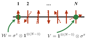
Figure 1: Spin-chain example: A spin chain exemplifies the quantum many-body systems characterized by the out-of-time-ordered correlator (OTOC). We illustrate with a one-dimensional chain of $N$ spin-$\frac{1}{2}$ degrees of freedom. The vertical red bars mark the sites. The dotted red arrows illustrate how spins can point in arbitrary directions. The OTOC is defined in terms of local unitary or Hermitian operators $\mathcal{W}$ and $V$. Example operators include single-qubit Paulis $\sigma^{x}$ and $\sigma^{z}$ that act nontrivially on opposite sides of the chain.

We will often suppose that $S$ occupies, or is initialized to, a state

$$\rho=\sum_{j}p_{j}\lvert j\rangle\!\langle j\rvert\in\mathcal{D}(\mathcal{H})\,.$$ (25)

The set of density operators defined on $\mathcal{H}$ is denoted by $\mathcal{D}(\mathcal{H})$, as in Sec. I.1. Orthonormal eigenstates are indexed by $j$; eigenvalues are denoted by $p_{j}$. Much literature focuses on temperature-$T$ thermal states $e^{-H/T}/Z$. (The partition function $Z$ normalizes the state.) We leave the form of $\rho$ general, as in YungerHalpern_17_Jarzynski .

The OTOC is defined in terms of local operators $\mathcal{W}$ and $V$. In the literature, $\mathcal{W}$ and $V$ are assumed to be unitary and/or Hermitian. Unitarity suffices for deriving the results in YungerHalpern_17_Jarzynski , as does Hermiticity. Unitarity and Hermiticity are assumed there, and here, for convenience. In our spin-chain example, the operators manifest as one-qubit Paulis that act nontrivially on opposite sides of the chain, e.g., $\mathcal{W}=\sigma^{z}\otimes\mathbbm{1}^{\otimes(N-1)}$, and $V=\mathbbm{1}^{\otimes(N-1)}\otimes\sigma^{x}$. In the Heisenberg Picture, $\mathcal{W}$ evolves as $\mathcal{W}(t):=U^{\dagger}\mathcal{W}U\,.$

The operators eigendecompose as

$$\mathcal{W}=\sum_{w_{\ell},\alpha_{w_{\ell}}}w_{\ell}\lvert w_{\ell},\alpha_{w_{\ell}}\rangle\!\langle w_{\ell},\alpha_{w_{\ell}}\rvert$$ (26)

and

$$V=\sum_{v_{\ell},\lambda_{v_{\ell}}}v_{\ell}\lvert v_{\ell},\lambda_{v_{\ell}}\rangle\!\langle v_{\ell},\lambda_{v_{\ell}}\rvert\,.$$ (27)

The eigenvalues are denoted by $w_{\ell}$ and $v_{\ell}$. The degeneracy parameters are denoted by $\alpha_{w_{\ell}}$ and $\lambda_{v_{\ell}}$. Recall that $\mathcal{W}$ and $V$ are local. In our example, $\mathcal{W}$ acts nontrivially on just one of $N\gg 1$ qubits. Hence $\mathcal{W}$ and $V$ are exponentially degenerate in $N$. The degeneracy parameters can be measured: Some nondegenerate Hermitian operator $\tilde{\mathcal{W}}$ has eigenvalues in a one-to-one correspondence with the $\alpha_{w_{\ell}}$’s. A measurement of $\mathcal{W}$ and $\tilde{\mathcal{W}}$ outputs a tuple $(w_{\ell},\alpha_{w_{\ell}})$. We refer to such a measurement as “a $\tilde{\mathcal{W}}$ measurement,” for conciseness. Analogous statements concern $V$ and a Hermitian operator $\tilde{V}$. Section II.1 introduces a trick that frees us from bothering with degeneracies.

I.3 The out-of-time-ordered correlator

Given two unitary operators $\mathcal{W}$ and $V$, the out-of-time-ordered correlator is defined as

$$F(t):=\langle\mathcal{W}^{\dagger}(t)V^{\dagger}\mathcal{W}(t)V\rangle\equiv\text{Tr}\bm{(}\rho\mathcal{W}^{\dagger}(t)V^{\dagger}\mathcal{W}(t)V\bm{)}\,.$$ (28)

This object reflects the degree of noncommutativity of $V$ and the Heisenberg operator $\mathcal{W}(t)$. More precisely, the OTOC appears in the expectation value of the squared magnitude of the commutator $[\mathcal{W}(t),V]$,

$$C(t):=\langle[\mathcal{W}(t),V]^{\dagger}[\mathcal{W}(t),V]\rangle=2-2\Re\bm{(}F(t)\bm{)}\,.$$ (29)

Even if $\mathcal{W}$ and $V$ commute, the Heisenberg operator $\mathcal{W}(t)$ generically does not commute with $V$ at sufficiently late times.

An analogous definition involves Hermitian $\mathcal{W}$ and $V$. The commutator’s square magnitude becomes

$$C(t)=-\langle[\mathcal{W}(t),V]^{2}\rangle.$$ (30)

This squared commutator involves TOC (time-ordered-correlator) and OTOC terms. The TOC terms take the forms $\langle V\mathcal{W}(t)\mathcal{W}(t)V\rangle$ and $\langle\mathcal{W}(t)VV\mathcal{W}(t)\rangle$. [Technically, $\langle V\mathcal{W}(t)\mathcal{W}(t)V\rangle$ is time-ordered. $\langle\mathcal{W}(t)VV\mathcal{W}(t)\rangle$ behaves similarly.]

The basic physical process reflected by the OTOC is the spread of Heisenberg operators with time. Imagine starting with a simple $\mathcal{W}$, e.g., an operator acting nontrivially on just one spin in a many-spin system. Time-evolving yields $\mathcal{W}(t)$. The operator has grown if $\mathcal{W}(t)$ acts nontrivially on more spins than $\mathcal{W}$ does. The operator $V$ functions as a probe for testing whether the action of $\mathcal{W}(t)$ has spread to the spin on which $V$ acts nontrivially.

Suppose $\mathcal{W}$ and $V$ are unitary and commute. At early times, $\mathcal{W}(t)$ and $V$ approximately commute. Hence $F(t)\approx 1$, and $C(t)\approx 0$. Depending on the dynamics, at later times, $\mathcal{W}(t)$ may significantly fail to commute with $V$. In a chaotic quantum system, $\mathcal{W}(t)$ and $V$ generically do not commute at late times, for most choices of $\mathcal{W}$ and $V$.

The analogous statement for Hermitian $\mathcal{W}$ and $V$ is that $F(t)$ approximately equals the TOC terms at early times. At late times, depending on the dynamics, the commutator can grow large. The time required for the TOC terms to approach their equilibrium values is called the dissipation time $t_{\text{d}}$. This time parallels the time required for a system to reach local thermal equilibrium. The time scale on which the commutator grows to be order-one is called the scrambling time $t_{*}$. The scrambling time parallels the time over which a drop of ink spreads across a container of water.

Why consider the commutator’s square modulus? The simpler object $\langle[\mathcal{W}(t),V]\rangle$ often vanishes at late times, due to cancellations between states in the expectation value. Physically, the vanishing of $\langle[\mathcal{W}(t),V]\rangle$ signifies that perturbing the system with $V$ does not significantly change the expectation value of $\mathcal{W}(t)$. This physics is expected for a chaotic system, which effectively loses its memory of its initial conditions. In contrast, $C(t)$ is the expectation value of a positive operator (the magnitude-squared commutator). The cancellations that zero out $\langle[\mathcal{W}(t),V]\rangle$ cannot zero out $\left\langle|[\mathcal{W}(t),V]|^{2}\right\rangle$.

Mathematically, the diagonal elements of the matrix that represents $[\mathcal{W}(t),V]$ relative to the energy eigenbasis can be small. $\left\langle[\mathcal{W}(t),V]\right\rangle$, evaluated on a thermal state, would be small. Yet the matrix’s off-diagonal elements can boost the operator’s Frobenius norm, $\sqrt{{\rm Tr}\left(|[\mathcal{W}(t),V]|^{2}\right)}$, which reflects the size of $C(t)$.

We can gain intuition about the manifestation of chaos in $F(t)$ from a simple quantum system that has a chaotic semiclassical limit. Let $\mathcal{W}=q$ and $\mathcal{V}=p$ for some position $q$ and momentum $p$:

$$C(t)=-\langle[q(t),p]^{2}\rangle\sim\hbar^{2}e^{2\lambda_{\rm L}t}\,.$$ (31)

This $\lambda_{\rm L}$ is a classical Lyapunov exponent. The final expression follows from the Correspondence Principle: Commutators are replaced with $i\hbar$ times the corresponding Poisson bracket. The Poisson bracket of $q(t)$ with $p$ equals the derivative of the final position with respect to the initial position. This derivative reflects the butterfly effect in classical chaos, i.e., sensitivity to initial conditions. The growth of $C(t)$, and the deviation of $F(t)$ from the TOC terms, provide a quantum generalization of the butterfly effect.

Within this simple quantum system, the analog of the dissipation time may be regarded as $t_{\text{d}}\sim\lambda_{\rm L}^{-1}$. The analog of the scrambling time is $t_{*}\sim\lambda_{\rm L}^{-1}\ln\frac{\Omega}{\hbar}$. The $\Omega$ denotes some measure of the accessible phase-space volume. Suppose that the phase space is large in units of $\hbar$. The scrambling time is much longer than the dissipation time: $t_{*}\gg t_{\rm d}$. Such a parametric separation between the time scales characterizes the systems that interest us most.

In more general chaotic systems, the value of $t_{*}$ depends on whether the interactions are geometrically local and on $\mathcal{W}$ and $V$. Consider, as an example, a spin chain governed by a local Hamiltonian. Suppose that $\mathcal{W}$ and $V$ are local operators that act nontrivially on spins separated by a distance $\ell$. The scrambling time is generically proportional to $\ell$. For this class of local models, $\ell/t_{*}$ defines a velocity $v_{\rm B}$ called the butterfly velocity. Roughly, the butterfly velocity reflects how quickly initially local Heisenberg operators grow in space.

Consider a system in which $t_{\rm d}$ is separated parametrically from $t_{*}$. The rate of change of $F(t)$ [rather, a regulated variation on $F(t)$] was shown to obey a nontrivial bound. Parameterize the OTOC as $F(t)\sim\text{TOC}-\epsilon\,e^{\lambda_{\rm L}t}$. The parameter $\epsilon\ll 1$ encodes the separation of scales. The exponent $\lambda_{\rm L}$ obeys $\lambda_{\rm L}\leq 2\pi k_{\mathrm{B}}T$ in thermal equilibrium at temperature $T$ Maldacena_15_Bound . $k_{\mathrm{B}}$ denotes Boltzmann’s constant. Black holes in the AdS/CFT duality saturate this bound, exhibiting maximal chaos Shenker_Stanford_14_BHs_and_butterfly ; Kitaev_15_Simple .

More generally, $\lambda_{\rm L}$ and $v_{\rm B}$ control the operators’ growth and the spread of chaos. The OTOC has thus attracted attention for a variety of reasons, including (but not limited to) the possibilities of nontrivial bounds on quantum dynamics, a new probe of quantum chaos, and a signature of black holes in AdS/CFT.

I.4 Introducing the quasiprobability behind the OTOC

$F(t)$ was shown, in YungerHalpern_17_Jarzynski , to equal a moment of a summed quasiprobability. We review this result, established in four steps: A quantum probability amplitude $A_{\rho}$ is reviewed in Sec. I.4.1 . Amplitudes are combined to form the quasiprobability $\tilde{A}_{\rho}$ in Sec. I.4.2. Summing $\tilde{A}_{\rho}(.)$ values, with constraints, yields a complex distribution $P(W,W^{\prime})$ in Sec. I.4.3. Differentiating $P(W,W^{\prime})$ yields the OTOC. $\tilde{A}_{\rho}$ can be inferred experimentally from a weak-measurement scheme and from interference. We review these schemes in Sec. I.4.4.

A third quasiprobability is introduced in Sec. II.1, the coarse-grained quasiprobability $\tilde{\mathscr{A}}_{\rho}$. $\tilde{\mathscr{A}}_{\rho}$ follows from summing values of $\tilde{A}_{\rho}$. $\tilde{\mathscr{A}}_{\rho}$ has a more concise description than $\tilde{A}_{\rho}$. Also, measuring $\tilde{\mathscr{A}}_{\rho}$ requires fewer resources (e.g., trials) than measuring $\tilde{A}_{\rho}$. Hence Sections II-IV will spotlight $\tilde{\mathscr{A}}_{\rho}$. $\tilde{A}_{\rho}$ returns to prominence in the proofs of Sec. V and in opportunities detailed in Sec. VI. Different distributions suit different investigations. Hence the presentation of three distributions in this thorough study: $\tilde{A}_{\rho}$, $\tilde{\mathscr{A}}_{\rho}$, and $P(W,W^{\prime})$.

I.4.1 Quantum probability amplitude $A_{\rho}$

The OTOC quasiprobability $\tilde{A}_{\rho}$ is defined in terms of probability amplitudes $A_{\rho}$. The $A_{\rho}$’s are defined in terms of the following process, $\mathscr{P}_{A}$:

1. Prepare $\rho$.

2. Measure the $\rho$ eigenbasis, $\left\{\lvert j\rangle\!\langle j\rvert\right\}$.

3. Evolve $S$ forward in time under $U$.

4. Measure $\tilde{\mathcal{W}}$.

5. Evolve $S$ backward under $U^{\dagger}$.

6. Measure $\tilde{V}$.

7. Evolve $S$ forward under $U$.

8. Measure $\tilde{\mathcal{W}}$.

Suppose that the measurements yield the outcomes $j$, $(w_{1},\alpha_{w_{1}})$, $(v_{1},\lambda_{v_{1}})$, and $(w_{2},\alpha_{w_{2}})$. Figure 2(a) illustrates this process. The process corresponds to the probability amplitude

$$A_{\rho}(j;w_{1},\alpha_{w_{1}};v_{1},\lambda_{v_{1}};w_{2},\alpha_{w_{2}}):=\langle w_{2},\alpha_{w_{2}}|U|v_{1},\lambda_{v_{1}}\rangle$$

$$\qquad\times\langle v_{1},\lambda_{v_{1}}|U^{\dagger}|w_{1},\alpha_{w_{1}}\rangle\langle w_{1},\alpha_{w_{1}}|U|j\rangle\sqrt{p_{j}}\,.$$ (32)

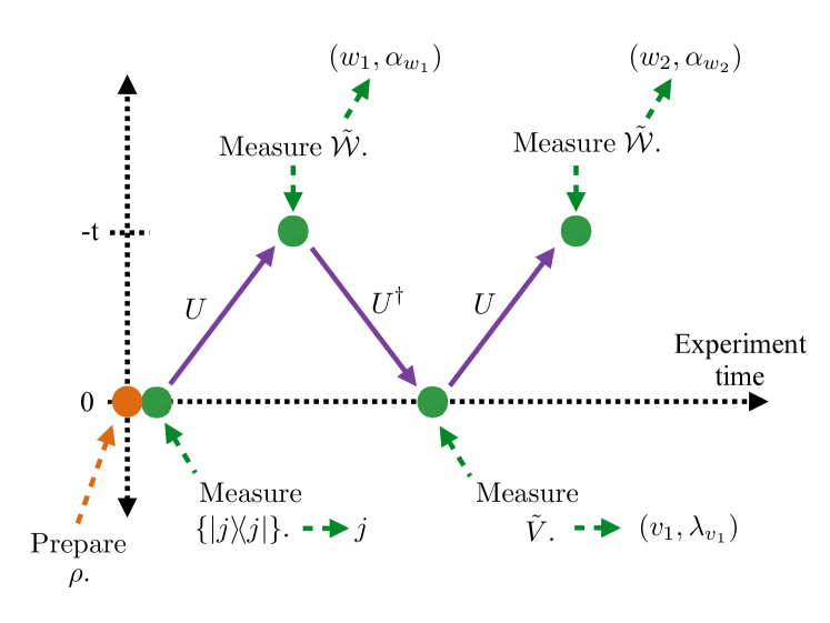
(a)

(b)

Figure 2: Quantum processes described by the probability amplitudes $A_{\rho}$ in the out-of-time-ordered correlator (OTOC): These figures, and parts of this caption, appear in YungerHalpern_17_Jarzynski . The OTOC quasiprobability $\tilde{A}_{\rho}$ results from summing products $A_{\rho}^{*}(.)A_{\rho}(.)$. Each $A_{\rho}(.)$ denotes a probability amplitude [Eq. (I.4.1)], so each product resembles a probability. But the amplitudes’ arguments differ—the amplitudes correspond to different quantum processes—because the OTOC operators $\mathcal{W}(t)$ and $V$ fail to commute, typically. Figure 2(a) illustrates the process described by the $A_{\rho}(.)$; and Fig. 2(b), the process described by the $A_{\rho}^{*}(.)$. Time, as measured by a laboratory clock, increases from left to right. Each process begins with the preparation of the state $\rho=\sum_{j}p_{j}\lvert j\rangle\!\langle j\rvert$ and a measurement of the state’s eigenbasis. Three evolutions ($U$, $U^{\dagger}$, and $U$) then alternate with three measurements of observables ($\tilde{\mathcal{W}}$, $\tilde{V}$, and $\tilde{\mathcal{W}}$). Figures 2(a) and 2(b) are used to define $\tilde{A}_{\rho}$, rather than showing protocols for measuring $\tilde{A}_{\rho}$.

We do not advocate for performing $\mathscr{P}_{A}$ in any experiment. $\mathscr{P}_{A}$ is used to define $A_{\rho}$ and to interpret $A_{\rho}$ physically. Instances of $A_{\rho}$ are combined into $\tilde{A}_{\rho}$. A weak-measurement protocol can be used to measure $\tilde{A}_{\rho}$ experimentally. An interference protocol can be used to measure $A_{\rho}$ (and so $\tilde{A}_{\rho}$) experimentally.

I.4.2 The fine-grained OTOC quasiprobability $\tilde{A}_{\rho}$

The quasiprobability’s definition is constructed as follows. Consider a realization of $\mathscr{P}_{A}$ that yields the outcomes $j$, $(w_{3},\alpha_{w_{3}})$, $(v_{2},\lambda_{v_{2}})$, and $(w_{2},\alpha_{w_{2}})$. Figure 2(b) illustrates this realization. The initial and final measurements yield the same outcomes as in the (I.4.1) realization. We multiply the complex conjugate of the second realization’s amplitude by the first realization’s probability amplitude. Then, we sum over $j$ and $(w_{1},\alpha_{w_{1}})$:^,

$$\tilde{A}_{\rho}(v_{1},\lambda_{v_{1}};w_{2},\alpha_{w_{2}};v_{2},\lambda_{v_{2}};w_{3},\alpha_{w_{3}})$$

$$:=\sum_{j,(w_{1},\alpha_{w_{1}})}A_{\rho}^{*}(j;w_{3},\alpha_{w_{3}};v_{2},\lambda_{v_{2}};w_{2},\alpha_{w_{2}})$$

$$\qquad\qquad\qquad\times A_{\rho}(j;w_{1},\alpha_{w_{1}};v_{1},\lambda_{v_{1}};w_{2},\alpha_{w_{2}})\,.$$ (33)

Equation (I.4.2) resembles a probability but differs due to the noncommutation of $\mathcal{W}(t)$ and $V$. We illustrate this relationship in two ways.

Consider a 1D quantum system, e.g., a particle on a line. We represent the system’s state with a wave function $\psi(x)$. The probability density at point $x$ equals $\psi^{*}(x)\,\psi(x)$. The $A^{*}_{\rho}\,A_{\rho}$ in Eq. (I.4.2) echoes $\psi^{*}\psi$. But the argument of the $\psi^{*}$ equals the argument of the $\psi$. The argument of the $A^{*}_{\rho}$ differs from the argument of the $A_{\rho}$, because $\mathcal{W}(t)$ and $V$ fail to commute.

Substituting into Eq. (I.4.2) from Eq. (I.4.1) yields

$$\tilde{A}_{\rho}(v_{1},\lambda_{v_{1}};w_{2},\alpha_{w_{2}};v_{2},\lambda_{v_{2}};w_{3},\alpha_{w_{3}})$$

$$=\langle w_{3},\alpha_{w_{3}}|U|v_{2},\lambda_{v_{2}}\rangle\langle v_{2},\lambda_{v_{2}}|U^{\dagger}|w_{2},\alpha_{w_{2}}\rangle$$

$$\qquad\times\langle w_{2},\alpha_{w_{2}}|U|v_{1},\lambda_{v_{1}}\rangle\langle v_{1},\lambda_{v_{1}}|\rho U^{\dagger}|w_{3},\alpha_{w_{3}}\rangle\,.$$ (34)

A simple example illustrates how $\tilde{A}_{\rho}$ nearly equals a probability. Suppose that an eigenbasis of $\rho$ coincides with $\left\{\lvert v_{\ell},\lambda_{v_{\ell}}\rangle\!\langle v_{\ell},\lambda_{v_{\ell}}\rvert\right\}$ or with $\left\{U^{\dagger}\lvert w_{\ell},\alpha_{w_{\ell}}\rangle\!\langle w_{\ell},\alpha_{w_{\ell}}\rvert U\right\}$. Suppose, for example, that

$$\rho=\rho_{V}:=\sum_{v_{\ell},\lambda_{v_{\ell}}}p_{v_{\ell},\lambda_{v_{\ell}}}\lvert v_{\ell},\lambda_{v_{\ell}}\rangle\!\langle v_{\ell},\lambda_{v_{\ell}}\rvert\,.$$ (35)

One such $\rho$ is the infinite-temperature Gibbs state $\mathbbm{1}/d$. Another example is easier to prepare: Suppose that $S$ consists of $N$ spins and that $V=\sigma^{x}_{N}$. One $\rho_{V}$ equals a product of $N$ $\sigma^{x}$ eigenstates. Let $(v_{2},\lambda_{v_{2}})=(v_{1},\lambda_{v_{1}})$. [An analogous argument follows from $(w_{3},\alpha_{w_{3}})=(w_{2},\alpha_{w_{2}})$.] Equation (I.4.2) reduces to

$$|\langle w_{2},\alpha_{w_{2}}|U|v_{1},\lambda_{v_{1}}\rangle|^{2}\,|\langle w_{3},\alpha_{w_{3}}|U|v_{1},\lambda_{v_{1}}\rangle|^{2}\,p_{v_{1},\lambda_{v_{1}}}\,.$$ (36)

Each square modulus equals a conditional probability. $p_{v_{1},\lambda_{v_{1}}}$ equals the probability that, if $\rho$ is measured with respect to $\left\{\lvert v_{\ell},\lambda_{v_{\ell}}\rangle\!\langle v_{\ell},\lambda_{v_{\ell}}\rvert\right\}$, outcome $(v_{1},\lambda_{v_{1}})$ obtains.

In this simple case, certain quasiprobability values equal probability values—the quasiprobability values that satisfy $(v_{2},\lambda_{v_{2}})=(v_{1},\lambda_{v_{1}})$ or $(w_{3},\alpha_{w_{3}})=(w_{2},\alpha_{w_{2}})$. When both conditions are violated, typically, the quasiprobability value does not equal a probability value. Hence not all the OTOC quasiprobability’s values reduce to probability values. Just as a quasiprobability lies behind the OTOC, quasiprobabilities lie behind time-ordered correlators (TOCs). Every value of a TOC quasiprobability reduces to a probability value in the same simple case (when $\rho$ equals, e.g., a $V$ eigenstate) (Sec. V.4).

I.4.3 Complex distribution $P(W,W^{\prime})$

$\tilde{A}_{\rho}$ is summed, in YungerHalpern_17_Jarzynski , to form a complex distribution $P(W,W^{\prime})$. Let $W:=w_{3}^{*}v_{2}^{*}$ and $W^{\prime}:=w_{2}v_{1}$ denote random variables calculable from measurement outcomes. If $\mathcal{W}$ and $V$ are Paulis, $(W,W^{\prime})$ can equal $(1,1),(1,-1),(-1,1),$ or $(-1,-1)$.

$W$ and $W^{\prime}$ serve, in the Jarzynski-like equality (1), analogously to thermodynamic work $W_{\rm th}$ in Jarzynski’s equality. $W_{\rm th}$ is a random variable, inferable from experiments, that fluctuates from trial to trial. So are $W$ and $W^{\prime}$. One infers a value of $W_{\rm th}$ by performing measurements and processing the outcomes. The two-point measurement scheme (TPMS) illustrates such protocols most famously. The TPMS has been used to derive quantum fluctuation relations Tasaki00 . One prepares the system in a thermal state, measures the Hamiltonian, $H_{i}$, projectively; disconnects the system from the bath; tunes the Hamiltonian to $H_{f}$; and measures $H_{f}$ projectively. Let $E_{i}$ and $E_{f}$ denote the measurement outcomes. The work invested in the Hamiltonian tuning is defined as $W_{\rm th}:=E_{f}-E_{i}$. Similarly, to infer $W$ and $W^{\prime}$, one can measure $\mathcal{W}$ and $V$ as in Sec. I.4.4, then multiply the outcomes.

Consider fixing the value of $(W,W^{\prime})$. For example, let $(W,W^{\prime})=(1,-1)$. Consider the octuples $(v_{1},\lambda_{v_{1}};w_{2},\alpha_{w_{2}};v_{2},\lambda_{v_{2}};w_{3},\alpha_{w_{3}})$ that satisfy the constraints $W=w_{3}^{*}v_{2}^{*}$ and $W^{\prime}=w_{2}v_{1}$. Each octuple corresponds to a quasiprobability value $\tilde{A}_{\rho}(.)$. Summing these quasiprobability values yields

$$P(W,W^{\prime}):=\sum_{\begin{subarray}{c}(v_{1},\lambda_{v_{1}}),(w_{2},\alpha_{w_{2}}),(v_{2},\lambda_{v_{2}}),(w_{3},\alpha_{w_{3}})\end{subarray}}$$ (37)

$$\tilde{A}_{\rho}(v_{1},\lambda_{v_{1}};w_{2},\alpha_{w_{2}};v_{2},\lambda_{v_{2}};w_{3},\alpha_{w_{3}})\>\delta_{W(w_{3}^{*}v_{2}^{*})}\delta_{W^{\prime}(w_{2}v_{1})}\,.$$

The Kronecker delta is represented by $\delta_{ab}$. $P(W,W^{\prime})$ functions analogously to the probability distribution, in the fluctuation-relation paper Jarzynski_97_Nonequilibrium , over values of thermodynamic work.

The OTOC equals a moment of $P(W,W^{\prime})$ [Eq. (1)], which equals a constrained sum over $\tilde{A}_{\rho}$ YungerHalpern_17_Jarzynski . Hence our labeling of $\tilde{A}_{\rho}$ as a “quasiprobability behind the OTOC.” Equation (37) expresses the useful, difficult-to-measure $F(t)$ in terms of a characteristic function of a (summed) quasiprobability, as Jarzynski Jarzynski_97_Nonequilibrium expresses a useful, difficult-to-measure free-energy difference $\Delta F$ in terms of a characteristic function of a probability. Quasiprobabilities reflect nonclassicality (contextuality) as probabilities do not; so, too, does $F(t)$ reflect nonclassicality (noncommutation) as $\Delta F$ does not.

The definition of $P$ involves arbitrariness: The measurable random variables, and $P$, may be defined differently. Alternative definitions, introduced in Sec. V.5, extend more robustly to OTOCs that encode more time reversals. All possible definitions share two properties: (i) The arguments $W$, etc. denote random variables inferable from measurement outcomes. (ii) $P$ results from summing $\tilde{A}_{\rho}(.)$ values subject to constraints $\delta_{ab}$.

$P(W,W^{\prime})$ resembles a work distribution constructed by Solinas and Gasparinetti (S&G) Jordan_chat ; Solinas_chat . They study fluctuation-relation contexts, rather than the OTOC. S&G propose a definition for the work performed on a quantum system Solinas_15_Full ; Solinas_16_Probing . The system is coupled weakly to detectors at a protocol’s start and end. The couplings are represented by constraints like $\delta_{W(w_{3}^{*}v_{2}^{*})}$ and $\delta_{W^{\prime}(w_{2}v_{1})}$. Suppose that the detectors measure the system’s Hamiltonian. Subtracting the measurements’ outcomes yields the work performed during the protocol. The distribution over possible work values is a quasiprobability. Their quasiprobability is a Husimi $Q$-function, whereas the OTOC quasiprobability is a KD distribution Solinas_16_Probing . Related frameworks appear in Alonso_16_Thermodynamics ; Miller_16_Time ; Elouard_17_Role . The relationship between those thermodynamics frameworks and our thermodynamically motivated OTOC framework merits exploration.

I.4.4 Weak-measurement and interference schemes for inferring $\tilde{A}_{\rho}$

$\tilde{A}_{\rho}$ can be inferred from weak measurements and from interference, as shown in YungerHalpern_17_Jarzynski . Section II.4 shows how to infer a coarse-graining of $\tilde{A}_{\rho}$ from other OTOC-measurement schemes (e.g., Swingle_16_Measuring ). We focus mostly on the weak-measurement scheme here. The scheme is simplified in Sec. II. First, we briefly review the interference scheme.

The interference scheme in YungerHalpern_17_Jarzynski differs from other interference schemes for measuring $F(t)$ Swingle_16_Measuring ; Yao_16_Interferometric ; Bohrdt_16_Scrambling : From the YungerHalpern_17_Jarzynski interference scheme, one can infer not only $F(t)$, but also $\tilde{A}_{\rho}$. Time need not be inverted ($H$ need not be negated) in any trial. The scheme is detailed in Appendix B of YungerHalpern_17_Jarzynski . The system is coupled to an ancilla prepared in a superposition $\frac{1}{\sqrt{2}}\,(\lvert 0\rangle+\lvert 1\rangle)$. A unitary, conditioned on the ancilla, rotates the system’s state. The ancilla and system are measured projectively. From many trials’ measurement data, one infers $\langle a|\mathcal{U}|b\rangle$, wherein $\mathcal{U}=U$ or $U^{\dagger}$ and $a,b=(w_{\ell},\alpha_{w_{\ell}}),(v_{m},\lambda_{v_{m}})$. These inner products are multiplied together to form $\tilde{A}_{\rho}$ [Eq. (I.4.2)]. If $\rho$ shares neither the $\tilde{V}$ nor the $\tilde{\mathcal{W}}(t)$ eigenbasis, quantum-state tomography is needed to infer $\langle v_{1},\lambda_{v_{1}}|\rho U^{\dagger}|w_{3},\alpha_{w_{3}}\rangle$.

The weak-measurement scheme is introduced in Sec. II B 3 of YungerHalpern_17_Jarzynski . A simple case, in which $\rho=\mathbbm{1}/d$, is detailed in Appendix A of YungerHalpern_17_Jarzynski . Recent weak measurements Bollen_10_Direct ; Lundeen_11_Direct ; Lundeen_12_Procedure ; Bamber_14_Observing ; Mirhosseini_14_Compressive ; White_16_Preserving ; Piacentini_16_Measuring ; Suzuki_16_Observation ; Thekkadath_16_Direct , some used to infer KD distributions, inspired our weak $\tilde{A}_{\rho}$-measurement proposal. We review weak measurements, a Kraus-operator model for measurements, and the $\tilde{A}_{\rho}$-measurement scheme.

Review of weak measurements: Measurements can alter quantum systems’ states. A weak measurement barely disturbs the measured system’s state. In exchange, the measurement provides little information about the system. Yet one can infer much by performing many trials and processing the outcome statistics.

Extreme disturbances result from strong measurements NielsenC10 . The measured system’s state collapses onto a subspace. For example, let $\rho$ denote the initial state. Let $\mathcal{A}=\sum_{a}a\lvert a\rangle\!\langle a\rvert$ denote the measured observable’s eigendecomposition. A strong measurement has a probability $\langle a|\rho|a\rangle$ of projecting $\rho$ onto $\lvert a\rangle$.

One can implement a measurement with an ancilla. Let $X=\sum_{x}x\lvert x\rangle\!\langle x\rvert$ denote an ancilla observable. One correlates $\mathcal{A}$ with $X$ via an interaction unitary. Von Neumann modeled such unitaries with $V_{\rm int}:=e^{-i\tilde{g}\,\mathcal{A}\otimes X}$ vonNeumann_32_Mathematische ; Dressel_15_Weak . The parameter $\tilde{g}$ signifies the interaction strength. An ancilla observable—say, $Y=\sum_{y}y\lvert y\rangle\!\langle y\rvert$—is measured strongly.

The greater the $\tilde{g}$, the stronger the correlation between $\mathcal{A}$ and $Y$. $\mathcal{A}$ is measured strongly if it is correlated with $Y$ maximally, if a one-to-one mapping interrelates the $y$’s and the $a$’s. Suppose that the $Y$ measurement yields $y$. We say that an $\mathcal{A}$ measurement has yielded some outcome $a_{y}$.

Suppose that $\tilde{g}$ is small. $\mathcal{A}$ is correlated imperfectly with $Y$. The $Y$-measurement outcome, $y$, provides incomplete information about $\mathcal{A}$. The value most reasonably attributable to $\mathcal{A}$ remains $a_{y}$. But a subsequent measurement of $\mathcal{A}$ would not necessarily yield $a_{y}$. In exchange for forfeiting information about $\mathcal{A}$, we barely disturb the system’s initial state. We can learn more about $\mathcal{A}$ by measuring $\mathcal{A}$ weakly in each of many trials, then processing measurement statistics.

Kraus-operator model for measurement: Kraus operators NielsenC10 model the system-of-interest evolution induced by a weak measurement. Let us choose the following form for $\mathcal{A}$. Let $V=\sum_{v_{\ell},\lambda_{v_{\ell}}}v_{\ell}\lvert v_{\ell},\lambda_{v_{\ell}}\rangle\!\langle v_{\ell},\lambda_{v_{\ell}}\rvert=\sum_{v_{\ell}}v_{\ell}\,\Pi^{V}_{v_{\ell}}$ denote an observable of the system. $\Pi^{V}_{v_{\ell}}$ projects onto the $v_{\ell}$ eigenspace. Let $\mathcal{A}=\lvert v_{\ell},\lambda_{v_{\ell}}\rangle\!\langle v_{\ell},\lambda_{v_{\ell}}\rvert$. Let $\rho$ denote the system’s initial state, and let $\lvert D\rangle$ denote the detector’s initial state.

Suppose that the $Y$ measurement yields $y$. The system’s state evolves under the Kraus operator

$$M_{y} =\langle y|V_{\rm int}|D\rangle$$ (38)

$$=\langle y|\exp\left(-i\tilde{g}\lvert v_{\ell},\lambda_{v_{\ell}}\rangle\!\langle v_{\ell},\lambda_{v_{\ell}}\rvert\otimes X\right)|D\rangle$$ (39)

$$=\langle y|D\rangle\,\mathbbm{1}$$

$$\quad+\langle y|\left(e^{-i\tilde{g}X}-\mathbbm{1}\right)|D\rangle\,\lvert v_{\ell},\lambda_{v_{\ell}}\rangle\!\langle v_{\ell},\lambda_{v_{\ell}}\rvert\,$$ (40)

as $\rho\mapsto\frac{M_{y}\rho M_{y}^{\dagger}}{{\rm Tr}\left(M_{y}\rho M_{y}^{\dagger}\right)}\,.$ The third equation follows from Taylor-expanding the exponential, then replacing the projector’s square with the projector. We reparameterize the coefficients as $\langle y|D\rangle\equiv p(y)\,e^{i\phi}$, wherein $p(y):=|\langle y|D\rangle|$, and $\langle y|\left(e^{-i\tilde{g}X}-\mathbbm{1}\right)|D\rangle\equiv g(y)\,e^{i\phi}$. An unimportant global phase is denoted by $e^{i\phi}$. We remove this global phase from the Kraus operator, redefining $M_{y}$ as

$$M_{y} =\sqrt{p(y)}\>\mathbbm{1}+g(y)\,\lvert v_{\ell},\lambda_{v_{\ell}}\rangle\!\langle v_{\ell},\lambda_{v_{\ell}}\rvert\,.$$ (42)

The coefficients have the following significances. Suppose that the ancilla did not couple to the system. The $Y$ measurement would have a baseline probability $p(y)$ of outputting $y$. The dimensionless parameter $g(y)\in\mathbb{C}$ is derived from $\tilde{g}$. We can roughly interpret $M_{y}$ statistically: In any given trial, the coupling has a probability $p(y)$ of failing to disturb the system (of evolving $\rho$ under $\mathbbm{1}$) and a probability $|g(y)|^{2}$ of projecting $\rho$ onto $\lvert v_{\ell},\lambda_{v_{\ell}}\rangle\!\langle v_{\ell},\lambda_{v_{\ell}}\rvert$.

Weak-measurement scheme for inferring the OTOC quasiprobability $\tilde{A}_{\rho}$: Weak measurements have been used to measure KD quasiprobabilities Bollen_10_Direct ; Lundeen_11_Direct ; Lundeen_12_Procedure ; Bamber_14_Observing ; Mirhosseini_14_Compressive ; White_16_Preserving ; Suzuki_16_Observation ; Thekkadath_16_Direct . These experiments’ techniques can be applied to infer $\tilde{A}_{\rho}$ and, from $\tilde{A}_{\rho}$, the OTOC. Our scheme involves three sequential weak measurements per trial (if $\rho$ is arbitrary) or two [if $\rho$ shares the $\tilde{V}$ or the $\tilde{\mathcal{W}}(t)$ eigenbasis, e.g., if $\rho=\mathbbm{1}/d$]. The weak measurements alternate with time evolutions and precede a strong measurement.

We review the general and simple-case protocols. A projection trick, introduced in Sec. II.1, reduces exponentially the number of trials required to infer about $\tilde{A}_{\rho}$ and $F(t)$. The weak-measurement and interference protocols are analyzed in Sec. II.2. A circuit for implementing the weak-measurement scheme appears in Sec. II.3.

Suppose that $\rho$ does not share the $\tilde{V}$ or the $\tilde{\mathcal{W}}(t)$ eigenbasis. One implements the following protocol, $\mathcal{P}$:

1. Prepare $\rho$.

2. Measure $\tilde{V}$ weakly. (Couple the system’s $\tilde{V}$ weakly to some observable $X$ of a clean ancilla. Measure $X$ strongly.)

3. Evolve the system forward in time under $U$.

4. Measure $\tilde{\mathcal{W}}$ weakly. (Couple the system’s $\tilde{\mathcal{W}}$ weakly to some observable $Y$ of a clean ancilla. Measure $Y$ strongly.)

5. Evolve the system backward under $U^{\dagger}$.

6. Measure $\tilde{V}$ weakly. (Couple the system’s $\tilde{V}$ weakly to some observable $Z$ of a clean ancilla. Measure $Z$ strongly.)

7. Evolve the system forward under $U$.

8. Measure $\tilde{\mathcal{W}}$ strongly.

$X$, $Y$, and $Z$ do not necessarily denote Pauli operators. Each trial yields three ancilla eigenvalues ($x$, $y$, and $z$) and one $\tilde{\mathcal{W}}$ eigenvalue ($w_{3},\alpha_{w_{3}}$). One implements $\mathcal{P}$ many times. From the measurement statistics, one infers the probability $\mathscr{P}_{\rm weak}(x;y;z;w_{3},\alpha_{w_{3}})$ that any given trial will yield the outcome quadruple $(x;y;z;w_{3},\alpha_{w_{3}})$.

From this probability, one infers the quasiprobability $\tilde{A}_{\rho}(v_{1},\lambda_{v_{1}};w_{2},\alpha_{w_{2}};v_{2},\lambda_{v_{2}};w_{3},\alpha_{w_{3}})$. The probability has the form

$$\mathscr{P}_{\rm weak}(x;y;z;w_{3},\alpha_{w_{3}})=\langle w_{3},\alpha_{w_{3}}\rvert UM_{z}U^{\dagger}M_{y}UM_{x}$$

$$\qquad\qquad\qquad\quad\times\rho M_{x}^{\dagger}U^{\dagger}M_{y}^{\dagger}UM_{z}^{\dagger}U^{\dagger}\lvert w_{3},\alpha_{w_{3}}\rangle\,.$$ (43)

We integrate over $x$, $y$, and $z$, to take advantage of all measurement statistics. We substitute in for the Kraus operators from Eq. (42), then multiply out. The result appears in Eq. (A7) of YungerHalpern_17_Jarzynski . Two terms combine into $\propto\Im\bm{(}\tilde{A}_{\rho}(.)\bm{)}$. The other terms form independently measurable “background” terms. To infer $\Re\bm{(}\tilde{A}_{\rho}(.)\bm{)}$, one performs $\mathcal{P}$ many more times, using different couplings (equivalently, measuring different detector observables). Details appear in Appendix A of YungerHalpern_17_Jarzynski .

To infer the OTOC, one multiplies each quasiprobability value $\tilde{A}_{\rho}(v_{1},\lambda_{v_{1}};w_{2},\alpha_{w_{2}};v_{2},\lambda_{v_{2}};w_{3},\alpha_{w_{3}})$ by the eigenvalue product $v_{1}w_{2}v_{2}^{*}w_{3}^{*}$. Then, one sums over the eigenvalues and the degeneracy parameters:

$$F(t) =\sum_{(v_{1},\lambda_{v_{1}}),(w_{2},\alpha_{w_{2}}),(v_{2},\lambda_{v_{2}}),(w_{3},\alpha_{w_{3}})}v_{1}w_{2}v_{2}^{*}w_{3}^{*}$$ (44)

$$\quad\times\tilde{A}_{\rho}(v_{1},\lambda_{v_{1}};w_{2},\alpha_{w_{2}};v_{2},\lambda_{v_{2}};w_{3},\alpha_{w_{3}})\,.$$

Equation (44) follows from Eq. (1). Hence inferring the OTOC from the weak-measurement scheme—inspired by Jarzynski’s equality—requires a few steps more than inferring a free-energy difference $\Delta F$ from Jarzynski’s equality Jarzynski_97_Nonequilibrium . Yet such quasiprobability reconstructions are performed routinely in quantum optics.

$\mathcal{W}$ and $V$ are local. Their degeneracies therefore scale with the system size. If $S$ consists of $N$ spin-$\frac{1}{2}$ degrees of freedom, $|\alpha_{w_{\ell}}|,|\lambda_{v_{\ell}}|\sim 2^{N}$. Exponentially many $\tilde{A}_{\rho}(.)$ values must be inferred. Exponentially many trials must be performed. We sidestep this exponentiality in Sec. II.1: One measures eigenprojectors of the degenerate $\mathcal{W}$ and $V$, rather than of the nondegenerate $\tilde{\mathcal{W}}$ and $\tilde{V}$. The one-dimensional $\lvert v_{\ell},\lambda_{v_{\ell}}\rangle\!\langle v_{\ell},\lambda_{v_{\ell}}\rvert$ of Eq. (I.4.4) is replaced with $\Pi^{V}_{v_{\ell}}$. From the weak measurements, one infers the coarse-grained quasiprobability $\sum_{\rm degeneracies}\tilde{A}_{\rho}(.)=:\tilde{\mathscr{A}}_{\rho}(.)$. Summing $\tilde{\mathscr{A}}_{\rho}(.)$ values yields the OTOC:

$$F(t) =\sum_{v_{1},w_{2},v_{2},w_{3}}v_{1}w_{2}v_{2}^{*}w_{3}^{*}\;\tilde{\mathscr{A}}_{\rho}(v_{1},w_{2},v_{2},w_{3})\,.$$ (45)

Equation (45) follows from performing the sums over the degeneracy parameters $\alpha$ and $\lambda$ in Eq. (44).

Suppose that $\rho$ shares the $\tilde{V}$ or the $\tilde{\mathcal{W}}(t)$ eigenbasis. The number of weak measurements reduces to two. For example, suppose that $\rho$ is the infinite-temperature Gibbs state $\mathbbm{1}/d$. The protocol $\mathcal{P}$ becomes

1. Prepare a $\tilde{\mathcal{W}}$ eigenstate $\lvert w_{3},\alpha_{w_{3}}\rangle$.

2. Evolve the system backward under $U^{\dagger}$.

3. Measure $\tilde{V}$ weakly.

4. Evolve the system forward under $U$.

5. Measure $\tilde{\mathcal{W}}$ weakly.

6. Evolve the system backward under $U^{\dagger}$.

7. Measure $\tilde{V}$ strongly.

In many recent experiments, only one weak measurement is performed per trial Bollen_10_Direct ; Lundeen_11_Direct ; Bamber_14_Observing . A probability $\mathscr{P}_{\rm weak}$ must be approximated to first order in the coupling constant $g(x)$. Measuring $\tilde{A}_{\rho}$ requires two or three weak measurements per trial. We must approximate $\mathscr{P}_{\rm weak}$ to second or third order. The more weak measurements performed sequentially, the more demanding the experiment. Yet sequential weak measurements have been performed recently Piacentini_16_Measuring ; Suzuki_16_Observation ; Thekkadath_16_Direct . The experimentalists aimed to reconstruct density matrices and to measure non-Hermitian operators. The OTOC measurement provides new applications for their techniques.

II Experimentally measuring $\tilde{A}_{\rho}$ and the coarse-grained $\tilde{\mathscr{A}}_{\rho}$

Multiple reasons motivate measurements of the OTOC quasiprobability $\tilde{A}_{\rho}$. $\tilde{A}_{\rho}$ is more fundamental than the OTOC $F(t)$, $F(t)$ results from combining values of $\tilde{A}_{\rho}$. $\tilde{A}_{\rho}$ exhibits behaviors not immediately visible in $F(t)$, as shown in Sections III and IV. $\tilde{A}_{\rho}$ therefore holds interest in its own right. Additionally, $\tilde{A}_{\rho}$ suggests new schemes for measuring the OTOC. One measures the possible values of $\tilde{A}_{\rho}(.)$, then combines the values to form $F(t)$. Two measurement schemes are detailed in YungerHalpern_17_Jarzynski and reviewed in Sec. I.4.4. One scheme relies on weak measurements; one, on interference. We simplify, evaluate, and augment these schemes.

First, we introduce a “projection trick”: Summing over degeneracies turns one-dimensional projectors (e.g., $\lvert w_{\ell},\alpha_{w_{\ell}}\rangle\!\langle w_{\ell},\alpha_{w_{\ell}}\rvert$) into projectors onto degenerate eigenspaces (e.g., $\Pi^{\mathcal{W}}_{w_{\ell}}$). The coarse-grained OTOC quasiprobability $\tilde{\mathscr{A}}_{\rho}$ results. This trick decreases exponentially the number of trials required to infer the OTOC from weak measurements. Section II.2 concerns pros and cons of the weak-measurement and interference schemes for measuring $\tilde{A}_{\rho}$ and $F(t)$. We also compare those schemes with alternative schemes for measuring $F(t)$. Section II.3 illustrates a circuit for implementing the weak-measurement scheme. Section II.4 shows how to infer $\tilde{\mathscr{A}}_{\rho}$ not only from the measurement schemes in Sec. I.4.4, but also with alternative OTOC-measurement proposals (e.g., Swingle_16_Measuring ) (if the eigenvalues of $\mathcal{W}$ and $V$ are $\pm 1$).

II.1 The coarse-grained OTOC quasiprobability $\tilde{\mathscr{A}}_{\rho}$ and a projection trick

$\mathcal{W}$ and $V$ are local. They manifest, in our spin-chain example, as one-qubit Paulis that nontrivially transform opposite ends of the chain. The operators’ degeneracies grows exponentially with the system size $N$: $|\alpha_{w_{\ell}}|,\>|\lambda_{v_{m}}|\sim 2^{N}$. Hence the number of $\tilde{A}_{\rho}(.)$ values grows exponentially. One must measure exponentially many numbers to calculate $F(t)$ precisely via $\tilde{A}_{\rho}$. We circumvent this inconvenience by summing over the degeneracies in $\tilde{A}_{\rho}(.)$, forming the coarse-grained quasiprobability $\tilde{\mathscr{A}}_{\rho}(.)$. $\tilde{\mathscr{A}}_{\rho}(.)$ can be measured in numerical simulations, experimentally via weak measurements, and (if the eigenvalues of $\mathcal{W}$ and $V$ are $\pm 1$) experimentally with other $F(t)$-measurement set-ups (e.g., Swingle_16_Measuring ).

The coarse-grained OTOC quasiprobability results from marginalizing $\tilde{A}_{\rho}(.)$ over its degeneracies:

$$\tilde{\mathscr{A}}_{\rho}(v_{1},w_{2},v_{2},w_{3}):=\sum_{\lambda_{v_{1}},\alpha_{w_{2}},\lambda_{v_{2}},\alpha_{w_{3}}}$$

$$\quad\tilde{A}_{\rho}(v_{1},\lambda_{v_{1}};w_{2},\alpha_{w_{2}};v_{2},\lambda_{v_{2}};w_{3},\alpha_{w_{3}})\,.$$ (46)

Equation (II.1) reduces to a more practical form. Consider substituting into Eq. (II.1) for $\tilde{A}_{\rho}(.)$ from Eq. (I.4.2). The right-hand side of Eq. (I.4.2) equals a trace. Due to the trace’s cyclicality, the three rightmost factors can be shifted leftward:

$$\tilde{\mathscr{A}}_{\rho}(v_{1},w_{2},v_{2},w_{3})=\sum_{\begin{subarray}{c}\lambda_{v_{1}},\alpha_{w_{2}},\\ \lambda_{v_{2}},\alpha_{w_{3}}\end{subarray}}{\rm Tr}\Big{(}\rho U^{\dagger}\lvert w_{3},\alpha_{w_{3}}\rangle\!\langle w_{3},\alpha_{w_{3}}\rvert U$$

$$\times\lvert v_{2},\lambda_{v_{2}}\rangle\!\langle v_{2},\lambda_{v_{2}}\rvert U^{\dagger}\lvert w_{2},\alpha_{w_{2}}\rangle\!\langle w_{2},\alpha_{w_{2}}\rvert U\lvert v_{1},\lambda_{v_{1}}\rangle\!\langle v_{1},\lambda_{v_{1}}\rvert\Big{)}\,.$$ (47)

The sums are distributed throughout the trace:

$$\tilde{\mathscr{A}}_{\rho}(v_{1},w_{2},v_{2},w_{3})={\rm Tr}\Bigg{(}\rho\Bigg{[}U^{\dagger}\sum_{\alpha_{w_{3}}}\lvert w_{3},\alpha_{w_{3}}\rangle\!\langle w_{3},\alpha_{w_{3}}\rvert U\Bigg{]}$$

$$\times\Bigg{[}\sum_{\lambda_{v_{2}}}\lvert v_{2},\lambda_{v_{2}}\rangle\!\langle v_{2},\lambda_{v_{2}}\rvert\Bigg{]}\Bigg{[}U^{\dagger}\sum_{\alpha_{w_{2}}}\lvert w_{2},\alpha_{w_{2}}\rangle\!\langle w_{2},\alpha_{w_{2}}\rvert U\Bigg{]}$$

$$\times\Bigg{[}\sum_{\lambda_{v_{1}}}\lvert v_{1},\lambda_{v_{1}}\rangle\!\langle v_{1},\lambda_{v_{1}}\rvert\Bigg{]}\Bigg{)}\,.$$ (48)

Define

$$\Pi^{\mathcal{W}}_{w_{\ell}}:=\sum_{\alpha_{w_{\ell}}}\lvert w_{\ell},\alpha_{w_{\ell}}\rangle\!\langle w_{\ell},\alpha_{w_{\ell}}\rvert$$ (49)

as the projector onto the $w_{\ell}$ eigenspace of $\mathcal{W}$,

$$\Pi^{\mathcal{W}(t)}_{w_{\ell}}:=U^{\dagger}\Pi^{\mathcal{W}}_{w_{\ell}}U$$ (50)

as the projector onto the $w_{\ell}$ eigenspace of $\mathcal{W}(t)$, and

$$\Pi^{V}_{v_{\ell}}:=\sum_{\lambda_{v_{\ell}}}\lvert v_{\ell},\lambda_{v_{\ell}}\rangle\!\langle v_{\ell},\lambda_{v_{\ell}}\rvert$$ (51)

as the projector onto the $v_{\ell}$ eigenspace of $V$. We substitute into Eq. (II.1), then invoke the trace’s cyclicality:

$$\boxed{\tilde{\mathscr{A}}_{\rho}(v_{1},w_{2},v_{2},w_{3})={\rm Tr}\Big{(}\Pi^{\mathcal{W}(t)}_{w_{3}}\Pi^{V}_{v_{2}}\Pi^{\mathcal{W}(t)}_{w_{2}}\Pi^{V}_{v_{1}}\rho\Big{)}}\,.$$ (52)

Asymmetry distinguishes Eq. (52) from Born’s Rule and from expectation values. Imagine preparing $\rho$, measuring $V$ strongly, evolving $S$ forward under $U$, measuring $\mathcal{W}$ strongly, evolving $S$ backward under $U^{\dagger}$, measuring $V$ strongly, evolving $S$ forward under $U$, and measuring $\mathcal{W}$. The probability of obtaining the outcomes $v_{1},w_{2},v_{2}$, and $w_{3}$, in that order, is

$${\rm Tr}\Big{(} \Pi^{\mathcal{W}(t)}_{w_{3}}\Pi^{V}_{v_{2}}\Pi^{\mathcal{W}(t)}_{w_{2}}\Pi^{V}_{v_{1}}\rho\Pi^{V}_{v_{1}}\Pi^{\mathcal{W}(t)}_{w_{2}}\Pi^{V}_{v_{2}}\Pi^{\mathcal{W}(t)}_{w_{3}}\Big{)}\,.$$ (53)

The operator $\Pi^{\mathcal{W}(t)}_{w_{3}}\Pi^{V}_{v_{2}}\Pi^{\mathcal{W}(t)}_{w_{2}}\Pi^{V}_{v_{1}}$ conjugates $\rho$ symmetrically. This operator multiplies $\rho$ asymmetrically in Eq. (52). Hence $\tilde{\mathscr{A}}_{\rho}$ does not obviously equal a probability.

Nor does $\tilde{\mathscr{A}}_{\rho}$ equal an expectation value. Expectation values have the form ${\rm Tr}(\rho\mathcal{A})$, wherein $\mathcal{A}$ denotes a Hermitian operator. The operator leftward of the $\rho$ in Eq. (52) is not Hermitian. Hence $\tilde{\mathscr{A}}_{\rho}$ lacks two symmetries of familiar quantum objects: the symmetric conjugation in Born’s Rule and the invariance, under Hermitian conjugation, of the observable $\mathcal{A}$ in an expectation value.

The right-hand side of Eq. (52) can be measured numerically and experimentally. We present numerical measurements in Sec. III. The weak-measurement scheme follows from Appendix A of YungerHalpern_17_Jarzynski , reviewed in Sec. I.4.4: Section I.4.4 features projectors onto one-dimensional eigenspaces, e.g., $\lvert v_{1},\lambda_{v_{1}}\rangle\!\langle v_{1},\lambda_{v_{1}}\rvert$. Those projectors are replaced with $\Pi$’s onto higher-dimensional eigenspaces. Section II.4 details how $\tilde{\mathscr{A}}_{\rho}$ can be inferred from alternative OTOC-measurement schemes.

II.2 Analysis of the quasiprobability-measurement schemes and comparison with other OTOC-measurement schemes

	Weak-	Yunger Halpern	Swingle	Yao	Zhu
	measurement	interferometry	et al.	et al.	et al.
Key tools	Weak	Interference	Interference,	Ramsey interfer.,	Quantum
	measurement		Lochschmidt echo	Rényi-entropy meas.	clock
What’s inferable	(1) $F(t)$, $\tilde{A}_{\rho}$,	$F^{(\bar{\mathscr{K}})}(t)$, $\tilde{A}_{\rho}^{\mathcal{K}}$,	$F(t)$	Regulated	$F(t)$
from the mea-	& $\rho$ or	& $\rho\;\>\forall\mathcal{K}$		correlator
surement?	(2) $F(t)$ & $\tilde{\mathscr{A}}_{\rho}$			$F_{\rm reg}(t)$
Generality	Arbitrary	Arbitrary	Arbitrary	Thermal:	Arbitrary
of $\rho$	$\rho\in\mathcal{D}(\mathcal{H})$	$\rho\in\mathcal{D}(\mathcal{H})$	$\rho\in\mathcal{D}(\mathcal{H})$	$e^{-H/T}/Z$	$\rho\in\mathcal{D}(\mathcal{H})$
Ancilla	Yes	Yes	Yes for $\Re\bm{(}F(t)\bm{)}$,	Yes	Yes
needed?			no for $|F(t)|^{2}$
Ancilla coup-	No	Yes	Yes	No	Yes
ling global?
How long must	1 weak	Whole	Whole	Whole	Whole
ancilla stay	measurement	protocol	protocol	protocol	protocol
coherent?
# time	2	0	1	0	2 (implemented
reversals					via ancilla)
# copies of $\rho$	1	1	1	2	1
needed / trial
Signal-to-	To be deter-	To be deter-	Constant	$\sim e^{-N}$	Constant
noise ratio	mined Swingle_Resilience	mined Swingle_Resilience	in $N$		in $N$
Restrictions	Hermitian or	Unitary	Unitary (extension	Hermitian	Unitary
on $\mathcal{W}$ & $V$	unitary		to Hermitian possible)	and unitary

Table 1: Comparison of our measurement schemes with alternatives: This paper focuses on the weak-measurement and interference schemes for measuring the OTOC quasiprobability $\tilde{A}_{\rho}$ or the coarse-grained quasiprobability $\tilde{\mathscr{A}}_{\rho}$. From $\tilde{A}_{\rho}$ or $\tilde{\mathscr{A}}_{\rho}$, one can infer the OTOC $F(t)$. These schemes appear in YungerHalpern_17_Jarzynski , are reviewed in Sec. I.4.4, and are assessed in Sec. II.2. We compare our schemes with the OTOC-measurement schemes in Swingle_16_Measuring ; Yao_16_Interferometric ; Zhu_16_Measurement . More OTOC-measurement schemes appear in Danshita_16_Creating ; Li_16_Measuring ; Garttner_16_Measuring ; Tsuji_17_Exact ; Campisi_16_Thermodynamics ; Bohrdt_16_Scrambling . Each row corresponds to a desirable quantity or to a resource potentially challenging to realize experimentally. The regulated correlator $F_{\rm reg}(t)$ [Eq. (108)] is expected to behave similarly to $F(t)$ Maldacena_15_Bound ; Yao_16_Interferometric . $\mathcal{D}(\mathcal{H})$ denotes the set of density operators defined on the Hilbert space $\mathcal{H}$. $\rho$ denotes the initially prepared state. Target states $\rho_{\rm target}$ are never prepared perfectly; $\rho$ may differ from $\rho_{\rm target}$. Experimentalists can reconstruct $\rho$ by trivially processing data taken to infer $\tilde{A}_{\rho}$ YungerHalpern_17_Jarzynski (Sec. V.2). $F^{(\bar{\mathscr{K}})}(t)$ denotes the $\bar{\mathscr{K}}$-fold OTOC, which encodes $\mathscr{K}=2\bar{\mathscr{K}}-1$ time reversals. The conventional OTOC corresponds to $\mathscr{K}=3$. The quasiprobability behind $F^{(\bar{\mathscr{K}})}(t)$ is $\tilde{A}_{\rho}^{(\mathscr{K})}$ (Sec. V.5). $N$ denotes the system size, e.g., the number of qubits. The Swingle et al. and Zhu et al. schemes have constant signal-to-noise ratios (SNRs) in the absence of environmental decoherence. The Yao et al. scheme’s SNR varies inverse-exponentially with the system’s entanglement entropy, $S_{\rm vN}$. The system occupies a thermal state $e^{-H/T}/Z$, so $S_{\rm vN}\sim\log(2^{N})=N$.

Section I.4.4 reviews two schemes for inferring $\tilde{A}_{\rho}$: a weak-measurement scheme and an interference scheme. From $\tilde{A}_{\rho}$ measurements, one can infer the OTOC $F(t)$. We evaluate our schemes’ pros and cons. Alternative schemes for measuring $F(t)$ have been proposed Swingle_16_Measuring ; Danshita_16_Creating ; Yao_16_Interferometric ; Zhu_16_Measurement ; Tsuji_17_Exact ; Campisi_16_Thermodynamics ; Bohrdt_16_Scrambling , and two schemes have been realized Li_16_Measuring ; Garttner_16_Measuring . We compare our schemes with alternatives, as summarized in Table 1. For specificity, we focus on Swingle_16_Measuring ; Yao_16_Interferometric ; Zhu_16_Measurement .

The weak-measurement scheme augments the set of techniques and platforms with which $F(t)$ can be measured. Alternative schemes rely on interferometry Swingle_16_Measuring ; Yao_16_Interferometric ; Bohrdt_16_Scrambling , controlled unitaries Swingle_16_Measuring ; Zhu_16_Measurement , ultracold-atoms tools Danshita_16_Creating ; Tsuji_17_Exact ; Bohrdt_16_Scrambling , and strong two-point measurements Campisi_16_Thermodynamics . Weak measurements, we have shown, belong in the OTOC-measurement toolkit. Such weak measurements are expected to be realizable, in the immediate future, with superconducting qubits White_16_Preserving ; Hacohen_16_Quantum ; Rundle_16_Quantum ; Takita_16_Demonstration ; Kelly_15_State ; Heeres_16_Implementing ; Riste_15_Detecting , trapped ions Gardiner_97_Quantum ; Choudhary_13_Implementation ; Lutterbach_97_Method ; Debnath_16_Nature ; Monz_16_Realization ; Linke_16_Experimental ; Linke_17_Experimental , cavity QED Guerlin_07_QND ; Murch_13_SingleTrajectories , ultracold atoms Browaeys_16_Experimental , and perhaps NMR Xiao_06_NMR ; Dawei_14_Experimental . Circuits for weakly measuring qubit systems have been designed Groen_13_Partial ; Hacohen_16_Quantum . Initial proof-of-principle experiments might not require direct access to the qubits: The five superconducting qubits available from IBM, via the cloud, might suffice IBM_QC . Random two-qubit unitaries could simulate chaotic Hamiltonian evolution.

In many weak-measurement experiments, just one weak measurement is performed per trial Lundeen_11_Direct ; Lundeen_12_Procedure ; Bamber_14_Observing ; Mirhosseini_14_Compressive . Yet two weak measurements have recently been performed sequentially Piacentini_16_Measuring ; Suzuki_16_Observation ; Thekkadath_16_Direct . Experimentalists aimed to “directly measure general quantum states” Lundeen_12_Procedure and to infer about non-Hermitian observable-like operators. The OTOC motivates a new application of recently realized sequential weak measurements.

Our schemes furnish not only the OTOC $F(t)$, but also more information:

1. From the weak-measurement scheme in YungerHalpern_17_Jarzynski , we can infer the following:

   1. The OTOC quasiprobability $\tilde{A}_{\rho}$. The quasiprobability is more fundamental than $F(t)$, as combining $\tilde{A}_{\rho}(.)$ values yields $F(t)$ [Eq. (44)].

   2. The OTOC $F(t)$.

   3. The form $\rho$ of the state prepared. Suppose that we wish to evaluate $F(t)$ on a target state $\rho_{\rm target}$. $\rho_{\rm target}$ might be difficult to prepare, e.g., might be thermal. The prepared state $\rho$ approximates $\rho_{\rm target}$. Consider performing the weak-measurement protocol $\mathcal{P}$ with $\rho$. One infers $\tilde{A}_{\rho}$. Summing $\tilde{A}_{\rho}(.)$ values yields the form of $\rho$. We can assess the preparation’s accuracy without performing tomography independently. Whether this assessment meets experimentalists’ requirements for precision remains to be seen. Details appear in Sec. V.3.

2. The weak-measurement protocol $\mathcal{P}$ is simplified later in this section. Upon implementing the simplified protocol, we can infer the following information:

   1. The coarse-grained OTOC quasiprobability $\tilde{\mathscr{A}}_{\rho}$. Though less fundamental than the fine-grained $\tilde{A}_{\rho}$, $\tilde{\mathscr{A}}_{\rho}$ implies the OTOC’s form [Eq. (45)].

   2. The OTOC $F(t)$.

3. Upon implementing the interferometry scheme in YungerHalpern_17_Jarzynski , we can infer the following information:

   1. The OTOC quasiprobability $\tilde{A}_{\rho}$.

   2. The OTOC $F(t)$.

   3. The form of the state $\rho$ prepared.

   4. All the $\bar{\mathscr{K}}$-fold OTOCs $F^{(\bar{\mathscr{K}})}(t)$, which generalize the OTOC $F(t)$. $F(t)$ encodes three time reversals. $F^{(\bar{\mathscr{K}})}(t)$ encodes $\mathscr{K}=2\bar{\mathscr{K}}-1=3,5,\ldots$ time reversals. Details appear in Sec. V.5.

   5. The quasiprobability $\tilde{A}_{\rho}^{(\mathscr{K})}$ behind $F^{(\bar{\mathscr{K}})}(t)$, for all $\mathscr{K}$ (Sec. V.5).

We have delineated the information inferable from the weak-measurement and interference schemes for measuring $\tilde{A}_{\rho}$ and $F(t)$. Let us turn to other pros and cons.

The weak-measurement scheme’s ancillas need not couple to the whole system. One measures a system weakly by coupling an ancilla to the system, then measuring the ancilla strongly. Our weak-measurement protocol requires one ancilla per weak measurement. Let us focus, for concreteness, on an $\tilde{\mathscr{A}}_{\rho}$ measurement for a general $\rho$. The protocol involves three weak measurements and so three ancillas. Suppose that $\mathcal{W}$ and $V$ manifest as one-qubit Paulis localized at opposite ends of a spin chain. Each ancilla need interact with only one site (Fig. 3). In contrast, the ancilla in Zhu_16_Measurement couples to the entire system. So does the ancilla in our interference scheme for measuring $\tilde{A}_{\rho}$. Global couplings can be engineered in some platforms, though other platforms pose challenges. Like our weak-measurement scheme, Swingle_16_Measuring and Yao_16_Interferometric require only local ancilla couplings.

In the weak-measurement protocol, each ancilla’s state must remain coherent during only one weak measurement—during the action of one (composite) gate in a circuit. The first ancilla may be erased, then reused in the third weak measurement. In contrast, each ancilla in Swingle_16_Measuring ; Yao_16_Interferometric ; Zhu_16_Measurement remains in use throughout the protocol. The Swingle et al. scheme for measuring $\Re\bm{(}F(t)\bm{)}$, too, requires an ancilla that remains coherent throughout the protocol Swingle_16_Measuring . The longer an ancilla’s “active-duty” time, the more likely the ancilla’s state is to decohere. Like the weak-measurement sheme, the Swingle et al. scheme for measuring $|F(t)|^{2}$ requires no ancilla Swingle_16_Measuring .

Also in the interference scheme for measuring $\tilde{A}_{\rho}$ YungerHalpern_17_Jarzynski , an ancilla remains active throughout the protocol. That protocol, however, is short: Time need not be reversed in any trial. Each trial features exactly one $U$ or $U^{\dagger}$, not both. Time can be difficult to reverse in some platforms, for two reasons. Suppose that a Hamiltonian $H$ generates a forward evolution. A perturbation $\varepsilon$ might lead $-(H+\varepsilon)$ to generate the reverse evolution. Perturbations can mar long-time measurements of $F(t)$ Zhu_16_Measurement . Second, systems interact with environments. Decoherence might not be completely reversible Swingle_16_Measuring . Hence the lack of a need for time reversal, as in our interference scheme and in Yao_16_Interferometric ; Zhu_16_Measurement , has been regarded as an advantage.

Unlike our interference scheme, the weak-measurement scheme requires that time be reversed. Perturbations $\varepsilon$ threaten the weak-measurement scheme as they threaten the Swingle et al. scheme Swingle_16_Measuring . $\varepsilon$’s might threaten the weak-measurement scheme more, because time is inverted twice in our scheme. Time is inverted only once in Swingle_16_Measuring . However, our error might be expected to have roughly the size of the Swingle et al. scheme’s error Swingle_Resilience . Furthermore, tools for mitigating the Swingle et al. scheme’s inversion error are being investigated Swingle_Resilience . Resilience of the Swingle et al. scheme to decoherence has been analyzed Swingle_16_Measuring . These tools may be applied to the weak-measurement scheme Swingle_Resilience . Like resilience, our schemes’ signal-to-noise ratios require further study.

As noted earlier, as the system size $N$ grows, the number of trials required to infer $\tilde{A}_{\rho}$ grows exponentially. So does the number of ancillas required to infer $\tilde{A}_{\rho}$: Measuring a degeneracy parameter $\alpha_{w_{\ell}}$ or $\lambda_{v_{m}}$ requires a measurement of each spin. Yet the number of trials, and the number of ancillas, required to measure the coarse-grained $\tilde{\mathscr{A}}_{\rho}$ remains constant as $N$ grows. One can infer $\tilde{\mathscr{A}}_{\rho}$ from weak measurements and, alternatively, from other $F(t)$-measurement schemes (Sec. II.4). $\tilde{\mathscr{A}}_{\rho}$ is less fundamental than $\tilde{A}_{\rho}$, as $\tilde{\mathscr{A}}_{\rho}$ results from coarse-graining $\tilde{A}_{\rho}$. $\tilde{\mathscr{A}}_{\rho}$, however, exhibits nonclassicality and OTOC time scales (Sec. III). Measuring $\tilde{\mathscr{A}}_{\rho}$ can balance the desire for fundamental knowledge with practicalities.

The weak-measurement scheme for inferring $\tilde{\mathscr{A}}_{\rho}$ can be rendered more convenient. Section II.1 describes measurements of projectors $\Pi$. Experimentalists might prefer measuring Pauli operators $\sigma^{\alpha}$. Measuring Paulis suffices for inferring a multiqubit system’s $\tilde{\mathscr{A}}_{\rho}$: The relevant $\Pi$ projects onto an eigenspace of a $\sigma^{\alpha}$. Measuring the $\sigma^{\alpha}$ yields $\pm 1$. These possible outcomes map bijectively onto the possible $\Pi$-measurement outcomes. See Footnote 10 for mathematics.

Our weak-measurement and interference schemes offer the advantage of involving general operators. $\mathcal{W}$ and $V$ must be Hermitian or unitary, not necessarily one or the other. Suppose that $\mathcal{W}$ and $V$ are unitary. Hermitian operators $G_{\mathcal{W}}$ and $G_{V}$ generate $\mathcal{W}$ and $V$, as discussed in Sec. I.2. $G_{\mathcal{W}}$ and $G_{V}$ may be measured in place of $\mathcal{W}$ and $V$. This flexibility expands upon the measurement opportunities of, e.g., Swingle_16_Measuring ; Yao_16_Interferometric ; Zhu_16_Measurement , which require unitary operators.

Our weak-measurement and interference schemes offer leeway in choosing not only $\mathcal{W}$ and $V$, but also $\rho$. The state can assume any form $\rho\in\mathcal{D}(\mathcal{H})$. In contrast, infinite-temperature Gibbs states $\rho=\mathbbm{1}/d$ were used in Li_16_Measuring ; Garttner_16_Measuring . Thermality of $\rho$ is assumed in Yao_16_Interferometric . Commutation of $\rho$ with $V$ is assumed in Campisi_16_Thermodynamics . If $\rho$ shares a $V$ eigenbasis or the $\mathcal{W}(t)$ eigenbasis, e.g., if $\rho=\mathbbm{1}/d$, our weak-measurement protocol simplifies from requiring three sequential weak measurements to requiring two.

II.3 Circuit for inferring $\tilde{\mathscr{A}}_{\rho}$ from weak measurements

Consider a 1D chain $S$ of $N$ qubits. A circuit implements the weak-measurement scheme reviewed in Sec. I.4.4. We exhibit a circuit for measuring $\tilde{\mathscr{A}}_{\rho}$. One subcircuit implements each weak measurement. These subcircuits result from augmenting Fig. 1 of Dressel_14_Implementing .

Dressel et al. use the partial-projection formalism, which we review first. We introduce notation, then review the weak-measurement subcircuit of Dressel_14_Implementing . Copies of the subcircuit are embedded into our $\tilde{\mathscr{A}}_{\rho}$-measurement circuit.

II.3.1 Partial-projection operators

Partial-projection operators update a state after a measurement that may provide incomplete information. Suppose that $S$ begins in a state $\lvert\psi\rangle$. Consider performing a measurement that could output $+$ or $-$. Let $\Pi_{+}$ and $\Pi_{-}$ denote the projectors onto the $+$ and $-$ eigenspaces. Parameters $p,q\in[0,1]$ quantify the correlation between the outcome and the premeasurement state. If $\lvert\psi\rangle$ is a $+$ eigenstate, the measurement has a probability $p$ of outputting $+$. If $\lvert\psi\rangle$ is a $-$ eigenstate, the measurement has a probability $q$ of outputting $-$.

Suppose that outcome $+$ obtains. We update $\lvert\psi\rangle$ using the partial-projection operator $D_{+}:=\sqrt{p}\;\Pi_{+}+\sqrt{1-q}\;\Pi_{-}$: $\lvert\psi\rangle\mapsto\frac{D_{+}\lvert\psi\rangle}{||D_{+}\lvert\psi\rangle||^{2}}\,.$ If the measurement yields $-$, we update $\lvert\psi\rangle$ with $D_{-}:=\sqrt{1-p}\;\Pi_{+}+\sqrt{q}\;\Pi_{-}$.

The measurement is strong if $(p,q)=(0,1)$ or $(1,0)$. $D_{+}$ and $D_{-}$ reduce to projectors. The measurement collapses $\lvert\psi\rangle$ onto an eigenspace. The measurement is weak if $p$ and $q$ lie close to $\frac{1}{2}$: $D_{\pm}$ lies close to the normalized identity, $\frac{\mathbbm{1}}{d}$. Such an operator barely changes the state. The measurement provides hardly any information.

We modeled measurements with Kraus operators $M_{x}$ in Sec. I.4.4. The polar decomposition of $M_{x}$ Preskill_15_Ch3 is a partial-projection operator. Consider measuring a qubit’s $\sigma^{z}$. Recall that $X$ denotes a detector observable. Suppose that, if an $X$ measurement yields $x$, a subsequent measurement of the spin’s $\sigma^{z}$ most likely yields $+$. The Kraus operator $M_{x}=\sqrt{p(x)}\>\mathbbm{1}+g(x)\,\Pi_{+}$ updates the system’s state. $M_{x}$ is related to $D_{+}$ by $D_{+}=U_{x}\sqrt{M_{x}^{\dagger}M_{x}}$ for some unitary $U_{x}$. The form of $U_{x}$ depends on the system-detector coupling and on the detector-measurement outcome.

The imbalance $|p-q|$ can be tuned experimentally. Our scheme has no need for a nonzero imbalance. We assume that $p$ equals $q$.

II.3.2 Notation

Let $\bm{\sigma}:=\sigma^{x}\,\hat{\mathbf{x}}+\sigma^{y}\,\hat{\mathbf{y}}+\sigma^{z}\,\hat{\mathbf{z}}$ denote a vector of one-qubit Pauli operators. The $\sigma^{z}$ basis serves as the computational basis in Dressel_14_Implementing . We will exchange the $\sigma^{z}$ basis with the $\mathcal{W}$ eigenbasis, or with the $V$ eigenbasis, in each weak-measurement subcircuit.

In our spin-chain example, $\mathcal{W}$ and $V$ denote one-qubit Pauli operators localized on opposite ends of the chain $S$: $\mathcal{W}=\sigma^{\mathcal{W}}\otimes\mathbbm{1}^{\otimes(N-1)}$, and $V=\mathbbm{1}^{\otimes(N-1)}\otimes\sigma^{V}$. Unit vectors $\hat{\mathcal{W}},\hat{V}\in\mathbb{R}^{3}$ are chosen such that $\sigma^{n}:=\bm{\sigma}\cdot\hat{\bm{n}}$, for $n=\mathcal{W},V$.

The one-qubit Paulis eigendecompose as $\sigma^{\mathcal{W}}=\lvert+\mathcal{W}\rangle\!\langle+\mathcal{W}\rvert-\lvert-\mathcal{W}\rangle\!\langle-\mathcal{W}\rvert$ and $\sigma^{V}=\lvert+V\rangle\!\langle+V\rvert-\lvert-V\rangle\!\langle-V\rvert$. The whole-system operators eigendecompose as $\mathcal{W}=\Pi^{\mathcal{W}}_{+}-\Pi^{\mathcal{W}}_{-}$ and $V=\Pi^{V}_{+}-\Pi^{V}_{-}$. A rotation operator $R_{n}$ maps the $\sigma^{z}$ eigenstates to the $\sigma^{n}$ eigenstates: $R_{n}\lvert+z\rangle=\lvert+n\rangle$, and $R_{n}\lvert-z\rangle=\lvert-n\rangle$.

We model weak $\mathcal{W}$ measurements with the partial-projection operators

$$D_{+}^{\mathcal{W}}:=\sqrt{p_{\mathcal{W}}}\;\Pi^{\mathcal{W}}_{+}+\sqrt{1-p_{\mathcal{W}}}\;\Pi^{\mathcal{W}}_{-}\;\>\text{and}$$ (54)

$$D_{-}^{\mathcal{W}}:=\sqrt{1-p_{\mathcal{W}}}\;\Pi^{\mathcal{W}}_{+}+\sqrt{p_{\mathcal{W}}}\;\Pi^{\mathcal{W}}_{-}\,.$$ (55)

The $V$ partial-projection operators are defined analogously:

$$D_{+}^{V}:=\sqrt{p_{V}}\;\Pi^{V}_{+}+\sqrt{1-p_{V}}\;\Pi^{V}_{-}\;\>\text{and}$$ (56)

$$D_{-}^{V}:=\sqrt{1-p_{V}}\;\Pi^{V}_{+}+\sqrt{p_{V}}\;\Pi^{V}_{-}\,.$$ (57)

II.3.3 Weak-measurement subcircuit

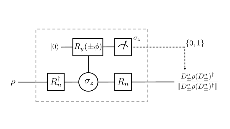
(a)

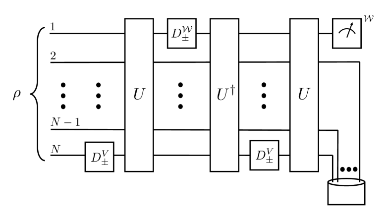
(b)

Figure 3: Quantum circuit for inferring the coarse-grained OTOC quasiprobability $\tilde{\mathscr{A}}_{\rho}$ from weak measurements: We consider a system of $N$ qubits prepared in a state $\rho$. The local operators $\mathcal{W}=\sigma^{\mathcal{W}}\otimes\mathbbm{1}^{\otimes(N-1)}$ and $V=\mathbbm{1}^{\otimes(N-1)}\otimes\sigma^{V}$ manifest as one-qubit Paulis. Weak measurements can be used to infer the coarse-grained quasiprobability $\tilde{\mathscr{A}}_{\rho}$. Combining values of $\tilde{\mathscr{A}}_{\rho}$ yields the OTOC $F(t)$. Figure 3(a) depicts a subcircuit used to implement a weak measurement of $n=\mathcal{W}$ or $V$. An ancilla is prepared in a fiducial state $\lvert 0\rangle$. A unitary $R_{n}^{\dagger}$ rotates the qubit’s $\sigma^{n}$ eigenbasis into its $\sigma^{z}$ eigenbasis. $R_{y}(\pm\phi)$ rotates the ancilla’s state counterclockwise about the $y$-axis through a small angle $\pm\phi$, controlled by the system’s $\sigma^{z}$. The angle’s smallness guarantees the measurement’s weakness. $R_{n}$ rotates the system’s $\sigma^{z}$ eigenbasis back into the $\sigma^{n}$ eigenbasis. The ancilla’s $\sigma^{z}$ is measured strongly. The outcome, $+$ or $-$, dictates which partial-projection operator $D_{\pm}^{n}$ updates the state. Figure 3(b) shows the circuit used to measure $\tilde{\mathscr{A}}_{\rho}$. Three weak measurements, interspersed with three time evolutions ($U$, $U^{\dagger}$, and $U$), precede a strong measurement. Suppose that the initial state, $\rho$, commutes with $\mathcal{W}$ or $V$, e.g., $\rho=\mathbbm{1}/d$. Figure 3(b) requires only two weak measurements.

Figure 3(a) depicts a subcircuit for measuring $n=\mathcal{W}$ or $V$ weakly. To simplify notation, we relabel $p_{n}$ as $p$. Most of the subcircuit appears in Fig. 1 of Dressel_14_Implementing . We set the imbalance parameter $\epsilon$ to 0. We sandwich Fig. 1 of Dressel_14_Implementing between two one-qubit unitaries. The sandwiching interchanges the computational basis with the $n$ eigenbasis.

The subcircuit implements the following algorithm:

1. Rotate the $n$ eigenbasis into the $\sigma^{z}$ eigenbasis, using $R_{n}^{\dagger}$.

2. Prepare an ancilla in a fiducial state $\lvert 0\rangle\equiv\lvert+z\rangle$.

3. Entangle $S$ with the ancilla via a $Z$-controlled-$Y$: If $S$ is in state $\lvert 0\rangle$, rotate the ancilla’s state counterclockwise (CCW) through a small angle $\phi\ll\frac{\pi}{2}$ about the $y$-axis. Let $R_{y}(\phi)$ denote the one-qubit unitary that implements this rotation. If $S$ is in state $\lvert 1\rangle$, rotate the ancilla’s state CCW through an angle $-\phi$, with $R_{y}(-\phi)$.

4. Measure the ancilla’s $\sigma^{z}$. If the measurement yields outcome $+$, $D_{+}$ updates the system’s state; and if $-$, then $D_{-}$.

5. Rotate the $\sigma^{z}$ eigenbasis into the $n$ eigenbasis, using $R_{n}$.

The measurement is weak because $\phi$ is small. Rotating through a small angle precisely can pose challenges White_16_Preserving .

II.3.4 Full circuit for weak-measurement scheme

Figure 3(b) shows the circuit for measuring $\tilde{\mathscr{A}}_{\rho}$. The full circuit contains three weak-measurement subcircuits. Each ancilla serves in only one subcircuit. No ancilla need remain coherent throughout the protocol, as discussed in Sec. II.2. The ancilla used in the first $V$ measurement can be recycled for the final $V$ measurement.

The circuit simplifies in a special case. Suppose that $\rho$ shares an eigenbasis with $V$ or with $\mathcal{W}(t)$, e.g., $\rho=\mathbbm{1}/d$. Only two weak measurements are needed, as discussed in Sec. I.4.4.

We can augment the circuit to measure $\tilde{A}_{\rho}$, rather than $\tilde{\mathscr{A}}_{\rho}$: During each weak measurement, every qubit will be measured. The qubits can be measured individually: The $N$-qubit measurement can be a product of local measurements. Consider, for concreteness, the first weak measurement. Measuring just qubit $N$ would yield an eigenvalue $v_{1}$ of $V$. We would infer whether qubit $N$ pointed upward or downward along the $\hat{V}$ axis. Measuring all the qubits would yield a degeneracy parameter $\lambda_{v_{1}}$. We could define $\lambda_{v_{\ell}}$ as encoding the $\hat{V}$-components of the other $N-1$ qubits’ angular momenta.

II.4 How to infer $\tilde{\mathscr{A}}_{\rho}$ from other OTOC-measurement schemes

$F(t)$ can be inferred, we have seen, from the quasiprobability $\tilde{A}_{\rho}$ and from the coarse-grained $\tilde{\mathscr{A}}_{\rho}$. $\tilde{\mathscr{A}}_{\rho}$ can be inferred from $F(t)$-measurement schemes, we show, if the eigenvalues of $\mathcal{W}$ and $V$ equal $\pm 1$. We assume, throughout this section, that they do. The eigenvalues equal $\pm 1$ if $\mathcal{W}$ and $V$ are Pauli operators.

The projectors (49) and (51) can be expressed as

$$\Pi^{\mathcal{W}}_{w_{\ell}}=\frac{1}{2}(\mathbbm{1}+w_{\ell}\mathcal{W})\quad\text{and}\quad\Pi^{V}_{v_{\ell}}=\frac{1}{2}(\mathbbm{1}+v_{\ell}V)\,.$$ (58)

Consider substituting from Eqs. (58) into Eq. (52). Multiplying out yields sixteen terms. If $\left\langle.\right\rangle:={\rm Tr}(.\,.)$,

$$\tilde{\mathscr{A}}_{\rho}(v_{1},w_{2},v_{2},w_{3})=\frac{1}{16}\Big{[}1+(w_{2}+w_{3})\left\langle\mathcal{W}(t)\right\rangle$$

$$+(v_{1}+v_{2})\left\langle V\right\rangle+w_{2}w_{3}\left\langle\mathcal{W}^{2}(t)\right\rangle+v_{1}v_{2}\left\langle V^{2}\right\rangle$$

$$+(w_{2}v_{1}+w_{3}v_{1}+w_{3}v_{2})\left\langle\mathcal{W}(t)V\right\rangle+w_{2}v_{2}\left\langle V\mathcal{W}(t)\right\rangle$$

$$+w_{2}w_{3}v_{1}\left\langle\mathcal{W}^{2}(t)V\right\rangle+w_{3}v_{1}v_{2}\left\langle\mathcal{W}(t)V^{2}\right\rangle$$

$$+w_{2}w_{3}v_{2}\left\langle\mathcal{W}(t)V\mathcal{W}(t)\right\rangle+w_{2}v_{1}v_{2}\left\langle V\mathcal{W}(t)V\right\rangle$$

$$+w_{2}w_{3}v_{1}v_{2}\,F(t)\Big{]}\,.$$ (59)

If $\mathcal{W}(t)$ and $V$ are unitary, they square to $\mathbbm{1}$. Equation (II.4) simplifies to

$$\tilde{\mathscr{A}}_{\rho}(v_{1},w_{2},v_{2},w_{3})=\frac{1}{16}\Big{\{}(1+w_{2}w_{3}+v_{1}v_{2})$$

$$+[w_{2}+w_{3}(1+v_{1}v_{2})]\left\langle\mathcal{W}(t)\right\rangle+[v_{1}(1+w_{2}w_{3})+v_{2}]\left\langle V\right\rangle$$

$$+(w_{2}v_{1}+w_{3}v_{1}+w_{3}v_{2})\left\langle\mathcal{W}(t)V\right\rangle+w_{2}v_{2}\left\langle V\mathcal{W}(t)\right\rangle$$

$$+w_{2}w_{3}v_{2}\left\langle\mathcal{W}(t)V\mathcal{W}(t)\right\rangle+w_{2}v_{1}v_{2}\left\langle V\mathcal{W}(t)V\right\rangle$$

$$+w_{2}w_{3}v_{1}v_{2}\,F(t)\Big{\}}\,.$$ (60)

The first term is constant. The next two terms are single-observable expectation values. The next two terms are two-point correlation functions. $\left\langle V\mathcal{W}(t)V\right\rangle$ and $\left\langle\mathcal{W}(t)V\mathcal{W}(t)\right\rangle$ are time-ordered correlation functions. $F(t)$ is the OTOC. $F(t)$ is the most difficult to measure. If one can measure it, one likely has the tools to infer $\tilde{\mathscr{A}}_{\rho}$. One can measure every term, for example, using the set-up in Swingle_16_Measuring .

III Numerical simulations

We now study the OTOC quasiprobability’s physical content in two simple models. In this section, we study a geometrically local 1D model, an Ising chain with transverse and longitudinal fields. In Sec. IV, we study a geometrically nonlocal model known as the Brownian-circuit model. This model effectively has a time-dependent Hamiltonian.

We compare the physics of $\tilde{\mathscr{A}}_{\rho}$ with that of the OTOC. The time scales inherent in $\tilde{\mathscr{A}}_{\rho}$, as compared to the OTOC’s time scales, particularly interest us. We study also nonclassical behaviors—negative and nonreal values—of $\tilde{\mathscr{A}}_{\rho}$. Finally, we find a parallel with classical chaos: The onset of scrambling breaks a symmetry. This breaking manifests in bifurcations of $\tilde{\mathscr{A}}_{\rho}$, reminiscent of pitchfork diagrams.

The Ising chain is defined on a Hilbert space of $N$ spin-$\frac{1}{2}$ degrees of freedom. The total Hilbert space has dimensionality $d=2^{N}$. The single-site Pauli matrices are labeled $\{\sigma^{x}_{i},\sigma^{y}_{i},\sigma^{z}_{i}\}$, for $i=1,...,N$. The Hamiltonian is

$$H=-J\sum_{i=1}^{N-1}\sigma_{i}^{z}\sigma_{i+1}^{z}-h\sum_{i=1}^{N}\sigma_{i}^{z}-g\sum_{i=1}^{N}\sigma^{x}_{i}\,.$$ (61)

The chain has open boundary conditions. Energies are measured in units of $J$. Times are measured in units of $1/J$. The interaction strength is thus set to one, $J=1$, henceforth. We numerically study this model for $N=10$ by exactly diagonalizing $H$. This system size suffices for probing the quasiprobability’s time scales. However, $N=10$ does not necessarily illustrate the thermodynamic limit.

When $h=0$, this model is integrable and can be solved with noninteracting-fermion variables. When $h\neq 0$, the model appears to be reasonably chaotic. These statements’ meanings are clarified in the data below. As expected, the quasiprobability’s qualitative behavior is sensitive primarily to whether $H$ is integrable, as well as to the initial state’s form. We study two sets of parameters,

Integrable: $$h=0,\>g=1.05\quad\text{and}$$

Nonintegrable: $$h=.5,\>g=1.05\,.$$ (62)

We study several classes of initial states $\rho$, including thermal states, random pure states, and product states.

For $\mathcal{W}$ and $V$, we choose single-Pauli operators that act nontrivially on just the chain’s ends. We illustrate with $\mathcal{W}=\sigma_{1}^{x}$ or $\mathcal{W}=\sigma_{1}^{z}$ and $V=\sigma_{N}^{x}$ or $\sigma_{N}^{z}$. These operators are unitary and Hermitian. They square to the identity, enabling us to use Eq. (II.4). We calculate the coarse-grained quasiprobability directly:

$$\tilde{\mathscr{A}}_{\rho}(v_{1},w_{2},v_{2},w_{3})=\text{Tr}\left(\rho\Pi^{\mathcal{W}(t)}_{w_{3}}\Pi^{V}_{v_{2}}\Pi^{\mathcal{W}(t)}_{w_{2}}\Pi^{V}_{v_{1}}\right)\,.$$ (63)

For a Pauli operator $\mathcal{O}$, $\Pi^{\mathcal{O}}_{a}=\frac{1}{2}\>(1+a\mathcal{O})$ projects onto the $a\in\{1,-1\}$ eigenspace. We also compare the quasiprobability with the OTOC, Eq. (45).

$F(t)$ deviates from one at roughly the time needed for information to propagate from one end of the chain to the other. This onset time, which up to a constant shift is also approximately the scrambling time, lies approximately between $t=4$ and $t=6$, according to our the data. The system’s length and the butterfly velocity $v_{\rm B}$ set the scrambling time (Sec. I.3). Every term in the Hamiltonian (61) is order-one. Hence $v_{\rm B}$ is expected to be order-one, too. In light of our spin chain’s length, the data below are all consistent with a $v_{\rm B}$ of approximately two.

III.1 Thermal states

We consider first thermal states $\rho\propto e^{-H/T}$. Data for the infinite-temperature ($T=\infty$) state, with $\mathcal{W}=\sigma_{1}^{z}$, $V=\sigma_{N}^{z}$, and nonintegrable parameters, appear in Figures 4, 5, and 6. The legend is labeled such that $abcd$ corresponds to $w_{3}=(-1)^{a}$, $v_{2}=(-1)^{b}$, $w_{2}=(-1)^{c}$, and $v_{1}=(-1)^{d}$. This labelling corresponds to the order in which the operators appear in Eq. (63).

Three behaviors merit comment. Generically, the coarse-grained quasiprobability is a complex number: $\tilde{\mathscr{A}}_{\rho}(.)\in\mathbb{C}$. However, $\tilde{\mathscr{A}}_{(\mathbbm{1}/d)}$ is real. The imaginary component $\Im\left(\tilde{\mathscr{A}}_{(\mathbbm{1}/d)}\right)$ might appear nonzero in Fig. 6. Yet $\Im\left(\tilde{\mathscr{A}}_{(\mathbbm{1}/d)}\right)\leq 10^{-16}$. This value equals zero, to within machine precision. The second feature to notice is that the time required for $\tilde{\mathscr{A}}_{(\mathbbm{1}/d)}$ to deviate from its initial value equals approximately the time required for the OTOC to deviate from its initial value. Third, although $\tilde{\mathscr{A}}_{(\mathbbm{1}/d)}$ is real, it is negative and hence nonclassical for some values of its arguments.

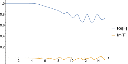
Figure 7: Real (upper curve) and imaginary (lower curve) parts of $F(t)$ as a function of time. $T=1$ thermal state. Nonintegrable parameters, $N=10$, $\mathcal{W}=\sigma_{1}^{z}$, $V=\sigma_{N}^{z}$.

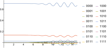
Figure 8: Real part of $\tilde{\mathscr{A}}_{\rho}$ as a function of time. $T=1$ thermal state. Nonintegrable parameters, $N=10$, $\mathcal{W}=\sigma_{1}^{z}$, $V=\sigma_{N}^{z}$. The upper curve includes $0000$, the middle curve includes $0011$, while the lower cluster of curves includes $0100$.

What about lower temperatures? Data for the $T=1$ thermal state are shown in Figures 7, 8, and 9. The coarse-grained quasiprobability is no longer real. Here, too, the time required for $\tilde{\mathscr{A}}_{\rho}$ to deviate significantly from its initial value is comparable with the time scale of changes in $F(t)$. This comparability characterizes the real and imaginary parts of $\tilde{\mathscr{A}}_{\rho}$. Both parts oscillate at long times. In the small systems considered here, such oscillations can arise from finite-size effects, including the energy spectrum’s discreteness. With nonintegrable parameters, this model has an energy gap $\Delta_{N=10}=2.92$ above the ground state. The temperature $T=1$ is smaller than the gap. Hence lowering $T$ from $\infty$ to 1 brings the thermal state close to the ground state.

What about long-time behavior? At infinite temperature, $\tilde{\mathscr{A}}_{(\mathbbm{1}/d)}$ approaches a limiting form after the scrambling time but before any recurrence time. Furthermore, $\tilde{\mathscr{A}}_{(\mathbbm{1}/d)}$ can approach one of only a few possible limiting values, depending on the function’s arguments. This behavior follows from the terms in Eq. (II.4). At infinite temperature, $\langle\mathcal{W}\rangle=\langle V\rangle=0$. Also the 3-point functions vanish, due to the trace’s cyclicity. We expect the nontrivial 2- and 4-point functions to be small at late times. (Such smallness is visible in the 4-point function in Fig. 4.) Hence Eq. (II.4) reduces as

$$\tilde{\mathscr{A}}_{\rho}(v_{1},w_{2},v_{2},w_{3})\underbrace{\longrightarrow}_{t\rightarrow\infty}\frac{1+w_{2}w_{3}+v_{1}v_{2}}{16}\,.$$ (64)

According to Eq. (64), the late-time values of $\tilde{\mathscr{A}}_{(\mathbbm{1}/d)}$ should cluster around $3/16$, $1/16$, and $-1/16$. This expectation is roughly consistent with Fig. 5, modulo the upper lines’ bifurcation.

A bifurcation of $\tilde{\mathscr{A}}_{\rho}$ signals the breaking of a symmetry at the onset of scrambling. Similarly, pitchfork plots signal the breaking of a symmetry in classical chaos Strogatz_00_Non . The symmetry’s mathematical form follows from Eq. (II.4). At early times, $\mathcal{W}(t)$ commutes with $V$, and $F(t)\approx 1$. Suppose, for simplicity, that $\rho=\mathbbm{1}/d$. The expectation values $\left\langle\mathcal{W}(t)\right\rangle$ and $\left\langle V\right\rangle$ vanish, because every Pauli has a zero trace. Equation (II.4) becomes

$$\tilde{\mathscr{A}}_{\rho}(v_{1},w_{2},v_{2},w_{3})=\frac{1}{16}\Big{[}(1+w_{2}w_{3}+v_{1}v_{2}+w_{2}w_{3}v_{1}v_{2})$$

$$\qquad\qquad\qquad+(w_{2}+w_{3})(v_{1}+v_{2})\left\langle\mathcal{W}(t)V\right\rangle\Big{]}\,.$$ (65)

Suppose that $w_{2}=-w_{3}$ and/or $v_{1}=-v_{2}$, as in the lower lines in Fig. 5. $\tilde{\mathscr{A}}_{\rho}(.)$ reduces to the constant

$$\frac{1}{16}(1+w_{2}w_{3}+v_{1}v_{2}+w_{2}w_{3}v_{1}v_{2})$$ (66)

$$=\frac{1}{32}\Big{[}(1+w_{2}w_{3}+v_{1}v_{2})^{2}-(w_{2}w_{3})^{2}-(v_{1}v_{2})^{2}+1\Big{]}\,.$$

The right-hand side depends on the eigenvalues $w_{\ell}$ and $v_{m}$ only through squares. $\tilde{\mathscr{A}}_{\rho}(.)$ remains invariant under the interchange of $w_{2}$ with $w_{3}$, under the interchange of $v_{1}$ with $v_{2}$, under the simultaneous negations of $w_{2}$ and $w_{3}$, and under the simultaneous negations of $v_{1}$ and $v_{2}$. These symmetries have operational significances: $\tilde{A}_{\rho}$ remains constant under permutations and negations of measurement outcomes in the weak-measurement scheme (Sec. I.4.4). Symmetries break as the system starts scrambling: $F(t)$ shrinks, shrinking the final term in Eq. (66). $\tilde{\mathscr{A}}_{\rho}$ starts depending not only on squares of $w_{\ell}$-and-$v_{m}$ functions, but also on the eigenvalues individually.

Whereas the shrinking of $F(t)$ bifurcates the lower lines in Fig. 5, the shrinking does not bifurcate the upper lines. The reason is that each upper line corresponds to $w_{2}w_{3}=v_{1}v_{2}=1$. [At early times, $|F(t)|$ is small enough that any $F(t)$-dependent correction would fall within the lines’ widths.] Hence the final term in Eq. (III.1) is proportional to $\pm\left\langle\mathcal{W}(t)V\right\rangle$. This prediction is consistent with the observed splitting. The $\left\langle\mathcal{W}(t)V\right\rangle$ term does not split the lower lines: Each lower line satisfies $w_{2}=-w_{3}$ and/or $v_{1}=-v_{2}$. Hence the $\left\langle\mathcal{W}(t)V\right\rangle$ term vanishes. We leave as an open question whether these pitchforks can be understood in terms of equilibria, like classical-chaos pitchforks Strogatz_00_Non .

In contrast with the $T=\infty$ data, the $T=1$ data oscillate markedly at late times (after the quasiprobability’s initial sharp change). We expect these oscillations to decay to zero at late times, if the system is chaotic, in the thermodynamic limit. Unlike at infinite temperature, $\mathcal{W}$ and $V$ can have nonzero expectation values. But, if all nontrivial connected correlation functions have decayed, Eq. (II.4) still implies a simple dependence on the $w_{\ell}$ and $v_{m}$ parameters at late times.

Finally, Figures 10 and 11 show the coarse-grained quasiprobability at infinite temperature, $\tilde{\mathscr{A}}_{(\mathbbm{1}/d)}$, with integrable parameters. The imaginary part remains zero, so we do not show it. The difference from the behavior in Figures 4 and 5 (which shows $T=\infty$, nonintegrable-$H$ data) is obvious. Most dramatic is the large revival that occurs at what would, in the nonintegrable model, be a late time. Although this is not shown, the quasiprobability depends significantly on the choice of operator. This dependence is expected, since different Pauli operators have different degrees of complexity in terms of the noninteracting-fermion variables.

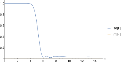
Figure 4: Real (upper curve) and imaginary (lower curve) parts of $F(t)$ as a function of time. $T=\infty$ thermal state. Nonintegrable parameters, $N=10$, $\mathcal{W}=\sigma_{1}^{z}$, $V=\sigma_{N}^{z}$.

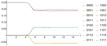
Figure 5: Real part of $\tilde{\mathscr{A}}_{\rho}$ as a function of time. $T=\infty$ thermal state. Nonintegrable parameters, $N=10$, $\mathcal{W}=\sigma_{1}^{z}$, $V=\sigma_{N}^{z}$. There are many degeneracies. The upper curves include $0000$ and $1010$, while the top of the lower pitchfork includes $1110$ and the bottom of the lower pitchfork includes $0001$.

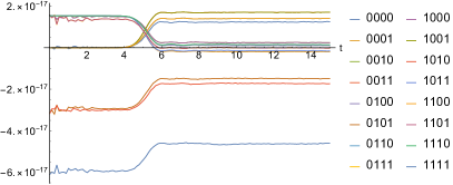
Figure 6: Imaginary part of $\tilde{\mathscr{A}}_{\rho}$ as a function of time. $T=\infty$ thermal state. Nonintegrable parameters, $N=10$, $\mathcal{W}=\sigma_{1}^{z}$, $V=\sigma_{N}^{z}$. To within machine precision, $\Im\left(\tilde{A}_{\rho}\right)$ vanishes for all values of the arguments.

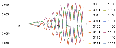
Figure 9: Imaginary part of $\tilde{\mathscr{A}}_{\rho}$ as a function of time. $T=1$ thermal state. Nonintegrable parameters, $N=10$, $\mathcal{W}=\sigma_{1}^{z}$, $V=\sigma_{N}^{z}$. The various curves display similar looking oscillations as a function of time; some of the curves appear to be more-or-less related by a factor of minus one, for example $1111$ and $1110$.

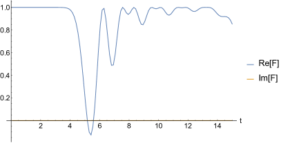
Figure 10: Real (upper curve) and imaginary (lower curve) parts of $F(t)$ as a function of time. $T=\infty$ thermal state. Integrable parameters, $N=10$, $\mathcal{W}=\sigma_{1}^{z}$, $V=\sigma_{N}^{z}$.

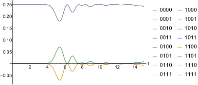
Figure 11: Real part of $\tilde{\mathscr{A}}_{\rho}$ as a function of time. $T=\infty$ thermal state. Integrable parameters, $N=10$, $\mathcal{W}=\sigma_{1}^{z}$, $V=\sigma_{N}^{z}$. Upper curve includes $0000$ while for the lower curves, the upper includes $1110$ and the lower includes $0001$.

III.2 Random states

We now consider random pure states $\rho\propto\lvert\psi\rangle\!\langle\psi\rvert$ and nonintegrable parameters. Figures 12, 13, and 14 show $F(t)$ and $\tilde{\mathscr{A}}_{\rho}$ for the operator choice $\mathcal{W}=\sigma_{1}^{z}$ and $V=\sigma_{N}^{z}$ in a randomly chosen pure state. The pure state is drawn according to the Haar measure. Each figure shows a single shot (contains data from just one pure state). Broadly speaking, the features are similar to those exhibited by the infinite-temperature $\rho=\mathbbm{1}/d$, with additional fluctuations.

The upper branch of lines in Fig. 13 exhibits dynamics before the OTOC does. However, lines’ average positions move significantly (the lower lines bifurcate, and the upper lines shift downward) only after the OTOC begins to evolve. The early motion must be associated with the early dynamics of the 2- and 3-point functions in Eq. (II.4). The late-time values are roughly consistent with those for $\rho=\mathbbm{1}/d$ but fluctuate more pronouncedly.

The agreement between random pure states and the $T=\infty$ thermal state is expected, due to closed-system thermalization D'Alessio_16_From ; Gogolin_16_Equilibration . Consider assigning a temperature to a pure state by matching its energy density with the energy density of the thermal state $e^{-H/T}/Z$, cast as a function of temperature. With high probability, any given random pure state corresponds to an infinite temperature. The reason is the thermodynamic entropy’s monotonic increase with temperature. Since the thermodynamic entropy gives the density of states, more states correspond to higher temperatures. Most states correspond to infinite temperature.

For the random states and system sizes $N$ considered, if $H$ is nonintegrable, the agreement with thermal results is not complete. However, the physics appears qualitatively similar.

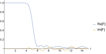
Figure 12: Real (upper curve) and imaginary (lower curve) parts of $F(t)$ as a function of time. Random pure state. Nonintegrable parameters, $N=10$, $\mathcal{W}=\sigma_{1}^{z}$, $V=\sigma_{N}^{z}$.

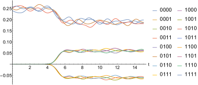
Figure 13: Real part of $\tilde{\mathscr{A}}_{\rho}$ as a function of time. Random pure state. Nonintegrable parameters, $N=10$, $\mathcal{W}=\sigma_{1}^{z}$, $V=\sigma_{N}^{z}$. The upper cluster includes $0000$ and $0011$. The upper prong of the lower pitchfork includes $1110$ while the lower prong includes $1001$.

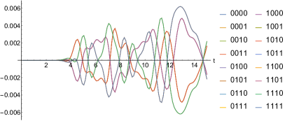
Figure 14: Imaginary part of $\tilde{\mathscr{A}}_{\rho}$ as a function of time. Random pure state. Nonintegrable parameters, $N=10$, $\mathcal{W}=\sigma_{1}^{z}$, $V=\sigma_{N}^{z}$. A familiar pattern of oscillations is visible, with some curves being more-or-less related by a factor of minus one, for example, $0011$ and $1000$.

III.3 Product states

Finally, we consider the product $\lvert+x\rangle^{\otimes N}$ of $N$ copies of the $+1$ $\sigma^{x}$ eigenstate (Figures 15–17). We continue to use $\mathcal{W}=\sigma_{1}^{z}$ and $V=\sigma_{N}^{z}$. For the Hamiltonian parameters chosen, this state lies far from the ground state. The state therefore should correspond to a large effective temperature. Figures 15, 16, and 17 show $F(t)$ and $\tilde{\mathscr{A}}_{\rho}$ for nonintegrable parameters.

The real part of $F(t)$ decays significantly from its initial value of one. The imaginary part of $F(t)$ is nonzero but remains small. These features resemble the infinite-temperature features. However, the late-time $F(t)$ values are substantially larger than in the $T=\infty$ case and oscillate significantly.

Correspondingly, the real and imaginary components of $\tilde{\mathscr{A}}_{\rho}$ oscillate significantly. $\Re\left(\tilde{\mathscr{A}}_{\rho}\right)$ exhibits dynamics before scrambling begins, as when $\rho$ is a random pure state. The real and imaginary parts of $\tilde{\mathscr{A}}_{\rho}$ differ more from their $T=\infty$ counterparts than $F(t)$ differs from its counterpart. Some of this differing is apparently washed out by the averaging needed to construct $F(t)$ [Eq. (45)].

We expected pure product states to behave roughly like random pure states. The data support this expectation very roughly, at best. Whether finite-size effects cause this deviation, we leave as a question for further study.

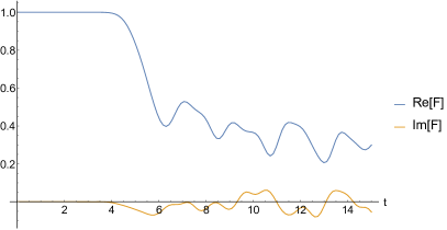
Figure 15: Real (upper curve) and imaginary (lower curve) parts of $F(t)$ as a function of time. Product $\lvert+x\rangle^{\otimes N}$ of $N$ copies of the $+1$ $\sigma^{x}$ eigenstate. Nonintegrable parameters, $N=10$, $\mathcal{W}=\sigma_{1}^{z}$, $V=\sigma_{N}^{z}$.

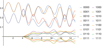
Figure 16: Real part of $\tilde{\mathscr{A}}_{\rho}$ as a function of time. Product $\lvert+x\rangle^{\otimes N}$ of $N$ copies of the $+1$ $\sigma^{x}$ eigenstate. Nonintegrable parameters, $N=10$, $\mathcal{W}=\sigma_{1}^{z}$, $V=\sigma_{N}^{z}$. The top of the upper cluster includes $0101$ while the bottom of the upper cluster includes $0011$. The top of the lower pitchfork includes $1110$ while the bottom of the lower pitchfork includes $1001$.

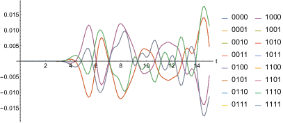
Figure 17: Imaginary part of $\tilde{\mathscr{A}}_{\rho}$ as a function of time. Product $\lvert+x\rangle^{\otimes N}$ of $N$ copies of the $+1$ $\sigma^{x}$ eigenstate. Nonintegrable parameters, $N=10$, $\mathcal{W}=\sigma_{1}^{z}$, $V=\sigma_{N}^{z}$. Similar physics to other depictions of the imaginary part.

III.4 Summary

The main messages from this study are the following.

1. The coarse-grained quasiprobability $\tilde{\mathscr{A}}_{\rho}$ is generically complex. Exceptions include the $T=\infty$ thermal state $\mathbbm{1}/d$ and states $\rho$ that share an eigenbasis with $V$ or with $\mathcal{W}(t)$ [e.g., as in Eq. (35)]. Recall that the KD distribution’s nonreality signals nonclassical physics (Sec. I.1).

2. The derived quantity $P(W,W^{\prime})$ is generically complex, our results imply. Nonclassicality thus survives even the partial marginalization that defines $P$ [Eq. (37)]. In general, marginalization can cause interference to dampen nonclassicality. (We observe such dampening in Property 6 of Sec. V.1 and in Property 9 of Appendix A.)

3. Random pure states’ quasiprobabilities resemble the $T=\infty$ thermal state’s quasiprobability but fluctuate more.

4. Certain product states’ quasiprobabilities display anomalously large fluctuations. We expected these states to resemble random states more.

5. The $\tilde{\mathscr{A}}_{\rho}$’s generated by integrable Hamiltonians differ markedly from the $\tilde{\mathscr{A}}_{\rho}$’s generated by nonintegrable Hamiltonians. Both types of $\tilde{\mathscr{A}}_{\rho}$’s achieve nonclassical values, however. We did not clearly observe a third class of behavior.

6. The time scale after which $\tilde{\mathscr{A}}_{\rho}$ changes significantly is similar to the OTOC time scale. $\tilde{\mathscr{A}}_{\rho}$ can display nontrivial early-time dynamics not visible in $F(t)$. This dynamics can arise, for example, because of the 2-point function contained in the expansion of $\tilde{\mathscr{A}}_{\rho}$ [see Eq. (II.4)].

7. $\tilde{\mathscr{A}}_{\rho}$ reveals that scrambling breaks a symmetry. Operationally, the symmetry consists of invariances of $\tilde{\mathscr{A}}_{\rho}$ under permutations and negations of measurement outcomes in the weak-measurement scheme (Sec. I.4.4). The symmetry breaking manifests in bifurcations of $\tilde{\mathscr{A}}_{\rho}$. These bifurcations evoke classical-chaos pitchfork diagrams, which also arise when a symmetry breaks. One equilibrium point splits into three in the classical case Strogatz_00_Non . Perhaps the quasiprobability’s pitchforks can be recast in terms of equilibria.

IV Calculation of $\tilde{\mathscr{A}}_{\rho}$ averaged over Brownian circuits

We study a geometrically nonlocal model—the Brownian-circuit model—governed by a time-dependent Hamiltonian Lashkari_13_Towards . We access physics qualitatively different from the physics displayed in the numerics of Sec. III. We also derive results for large systems and compare with the finite-size numerics. Since the two models’ locality properties differ, we do not expect agreement at early times. The late-time scrambled states, however, may be expected to share similarities. We summarize our main findings at the end of the section.

We consider a system of $N$ qubits governed by the random time-dependent Hamiltonian

$$H(t)\propto\sum_{i<j}\sum_{\alpha_{i},\alpha_{j}}J^{\alpha_{i},\alpha_{j}}_{i,j}(t)\,\sigma_{i}^{\alpha_{i}}\sigma_{j}^{\alpha_{j}}\,.$$ (67)

The couplings $J$ are time-dependent random variables. We denote the site-$i$ identity operator and Pauli operators by $\sigma_{i}^{\alpha}$, for $\alpha=0,1,2,3$. According to the model’s precise formulation, the time-evolution operator $U(t)$ is a random variable that obeys

$$U(t+dt) -U(t)=-\frac{N}{2}U(t)dt-i\,dB(t)\,.$$ (68)

The final term’s $dB(t)$ has the form

$$dB(t)=\sqrt{\frac{1}{8(N-1)}}\sum_{i<j}\sum_{\alpha_{i},\alpha_{j}}\sigma_{i}^{\alpha_{i}}\sigma_{j}^{\alpha_{j}}dB^{\alpha_{i},\alpha_{j}}_{i,j}(t)\,.$$ (69)

We will sometimes call Eq. (69) “$dB$.” $dB$ is a Gaussian random variable with zero mean and with variance

$$\mathbf{E}_{B}\left\{dB^{\alpha,\beta}_{i,j}\,dB^{\alpha^{\prime},\beta^{\prime}}_{i^{\prime},j^{\prime}}\right\}=\delta_{\alpha,\alpha^{\prime}}\delta_{\beta,\beta^{\prime}}\delta_{i,i^{\prime}}\delta_{j,j^{\prime}}\,dt.$$ (70)

The expectation value $\mathbf{E}_{B}$ is an average over realizations of the noise $B$. We demand that $dt\,dt=0$ and $dB\,dt=0$, in accordance with the standard Ito calculus. $dB(t)$ is independent of $U(t)$, i.e., of all previous $dB$’s.

We wish to compute the average, over the ensemble defined by Eq. (68), of the coarse-grained quasiprobability:

$$\mathfrak{A}(v_{1},w_{2},v_{2},w_{3})=\mathbf{E}_{B}\left\{\tilde{\mathscr{A}}_{\rho}(v_{1},w_{2},v_{2},w_{3})\right\}\,.$$ (71)

IV.1 Infinite-temperature thermal state $\mathbbm{1}/2^{N}$

We focus here on the infinite-temperature thermal state, $\rho=\mathbbm{1}/2^{N}$, for two reasons. First, a system with a time-dependent Hamiltonian generically heats to infinite temperature with respect to any Hamiltonian in the ensemble. Second, the $T=\infty$ state is convenient for calculations. A discussion of other states follows.

The ensemble remains invariant under single-site rotations, and all qubits are equivalent. Therefore, all possible choices of single-site Pauli operators for $\mathcal{W}$ and $V$ are equivalent. Hence we choose $\mathcal{W}=\sigma_{1}^{z}$ and $V=\sigma_{2}^{z}$ without loss of generality.

Let us return to Eq. (II.4). Equation (II.4) results from substituting in for the projectors in $\tilde{\mathscr{A}}_{\rho}$. The sum contains $16$ terms. To each term, each projector contributes the identity $\mathbbm{1}$ or a nontrivial Pauli ($\mathcal{W}$ or $V$). The terms are

1. $\mathbbm{1}\mathbbm{1}\mathbbm{1}\mathbbm{1}$: $\text{Tr}\left\{\frac{\mathbbm{1}}{2^{N}}\right\}=1$,

2. $\mathcal{W}\mathbbm{1}\mathbbm{1}\mathbbm{1}$, $\mathbbm{1}V\mathbbm{1}\mathbbm{1}$, $\mathbbm{1}\mathbbm{1}\mathcal{W}\mathbbm{1}$, $\mathbbm{1}\mathbbm{1}\mathbbm{1}V$: $0$,

3. $\mathcal{W}V\mathbbm{1}\mathbbm{1}$, $\mathcal{W}\mathbbm{1}\mathbbm{1}V$, $\mathbbm{1}V\mathcal{W}\mathbbm{1}$, $\mathbbm{1}\mathbbm{1}\mathcal{W}V$:
   $\text{Tr}\left\{\frac{\sigma_{1}^{z}(t)\sigma_{2}^{z}}{2^{N}}\right\}=:G(t)$,

4. $\mathcal{W}\mathbbm{1}\mathcal{W}\mathbbm{1}$, $\mathbbm{1}V\mathbbm{1}V$: $\text{Tr}\left\{\frac{\mathbbm{1}}{2^{N}}\right\}=1$,

5. $\mathcal{W}V\mathcal{W}\mathbbm{1}$, $\mathcal{W}V\mathbbm{1}V$, $\mathcal{W}\mathbbm{1}\mathcal{W}V$, $\mathbbm{1}V\mathcal{W}V$: $0$,  and

6. $\mathcal{W}V\mathcal{W}V$: $\text{Tr}\left\{\frac{\sigma_{1}^{z}(t)\sigma_{2}^{z}\sigma_{1}^{z}(t)\sigma_{2}^{z}}{2^{N}}\right\}=F(t)$.

These computations rely on $\rho=\mathbbm{1}/2^{N}$. Each term that contains an odd number of Pauli operators vanishes, due to the trace’s cyclicality and to the Paulis’ tracelessness. We have introduced a 2-point function $G(t)$. An overall factor of $1/16$ comes from the projectors’ normalization.

Combining all the ingredients, we can express $\tilde{\mathscr{A}}_{\rho}$ in terms of $G$ and $F$. The result is

$$16\,\tilde{\mathscr{A}}_{\rho}(v_{1},w_{2},v_{2},w_{3})=(1+w_{2}w_{3}+v_{1}v_{2})$$ (72)

$$\qquad+(w_{2}+w_{3})(v_{1}+v_{2})\,G+w_{2}w_{3}v_{1}v_{2}\,F.$$

This result depends on $\rho=\mathbbm{1}/2^{N}$, not on the form of the dynamics. But to compute $\mathfrak{A}$, we must compute

$$\mathfrak{G}=\mathbf{E}_{B}\left\{G\right\}$$ (73)

and

$$\mathfrak{F}=\mathbf{E}_{B}\left\{F\right\}.$$ (74)

The computation of $\mathfrak{F}$ appears in the literature Shenker_Stanford_15_Stringy . $\mathfrak{F}$ initially equals unity. It decays to zero around $t_{*}=\frac{1}{3}\log N$, the scrambling time. The precise functional form of $\mathfrak{F}$ is not crucial. The basic physics is captured in a phenomenological form inspired by AdS/CFT computations Shenker_Stanford_15_Stringy ,

$$\mathfrak{F}\sim\left(\frac{1+c_{1}}{1+c_{1}e^{3t}}\right)^{c_{2}},$$ (75)

wherein $c_{1}\sim 1/N$ and $c_{2}\sim 1$.

To convey a sense of the physics, we review the simpler calculation of $\mathfrak{G}$. The two-point function evolves according to

$$G(t+dt) =\frac{1}{2^{N}}\>\text{Tr}\bigg{\{}\left[U(t)-\frac{N}{2}U(t)dt-i\,dB\,U(t)\right]\sigma_{1}^{z}$$

$$\times\left[U(t)^{\dagger}-\frac{N}{2}U(t)^{\dagger}dt+i\,U(t)^{\dagger}dB^{\dagger}\right]\sigma_{2}^{z}\bigg{\}}\,.$$ (76)

Using the usual rules of Ito stochastic calculus, particularly Eq. (70) and $dt\,dt=dB\,dt=0$, we obtain

$$\mathfrak{G}(t+dt)-\mathfrak{G}(t)=-N\,dt\,\mathfrak{G}(t)+dt\,\frac{1}{8(N-1)}$$

$$\times\sum_{i<j}\sum_{\alpha_{i},\alpha_{j}}\frac{1}{2^{N}}\mathbf{E}_{B}\left\{\text{Tr}\left\{\sigma_{1}^{z}(t)\sigma_{i}^{\alpha_{i}}\sigma_{j}^{\alpha_{j}}\sigma_{2}^{z}\sigma_{i}^{\alpha_{i}}\sigma_{j}^{\alpha_{j}}\right\}\right\}.$$ (77)

We have applied the trace’s cyclicality in the second term.

The second term’s value depends on whether $i$ and/or $j$ equals $2$. If $i$ and/or $j$ equals $2$, the second term vanishes because $\sum_{\alpha=0}^{3}\sigma^{\alpha}\sigma^{z}\sigma^{\alpha}=0$. If neither $i$ nor $j$ is $2$, $\sigma_{i}^{\alpha_{i}}\sigma_{j}^{\alpha_{j}}$ commutes with $\sigma_{2}^{z}$. The second term becomes proportional to $G$. In $(N-1)(N-2)/2$ terms, $i,j\neq 2$. An additional factor of $4^{2}=16$ comes from the two sums over Pauli matrices. Hence

$$\mathfrak{G}(t+dt)-\mathfrak{G}(t)=-2dt\,\mathfrak{G}\,,$$ (78)

or

$$\frac{d\mathfrak{G}}{dt}=-2\mathfrak{G}.$$ (79)

This differential equation implies that $\mathfrak{G}$ exponentially decays from its initial value. The initial value is zero: $\mathfrak{G}(0)=G(0)=0$. Hence $\mathfrak{G}(t)$ is identically zero.

Although it does not arise when we consider $\mathfrak{A}$, the ensemble-average autocorrelation function $\mathbf{E}_{B}\left\{\langle\sigma_{1}^{z}(t)\sigma_{1}^{z}\rangle\right\}$ obeys a differential equation similar to the equation obeyed by $\mathfrak{G}$. In particular, the equation decays exponentially with an order-one rate.

By the expectation value’s linearity and the vanishing of $\mathfrak{G}$,

$$\mathfrak{A}=\frac{(1+w_{2}w_{3}+v_{1}v_{2})+w_{2}w_{3}v_{1}v_{2}\,\mathfrak{F}}{16}.$$ (80)

This simple equation states that the ensemble-averaged quasiprobability depends only on the ensemble-averaged OTOC $F(t)$, at infinite temperature. The time scale of $\mathfrak{F}$’s decay is $t_{*}=\frac{1}{3}\log N$. Hence this is the time scale of changes in $\mathfrak{A}$.

Equation (80) shows (as intuition suggests) that $\mathfrak{A}$ depends only on the combinations $w_{2}w_{3}$ and $v_{1}v_{2}$. At $t=0$, $\mathfrak{F}(0)=1$. Hence $\mathfrak{A}$ is

$$\mathfrak{A}_{t=0}=\frac{1+w_{2}w_{3}+v_{1}v_{2}+w_{2}w_{3}v_{1}v_{2}}{16}.$$ (81)

The cases are

1. $w_{2}w_{3}=1,v_{1}v_{2}=1$: $\mathfrak{A}=1/4$,

2. $w_{2}w_{3}=1,v_{1}v_{2}=-1$: $\mathfrak{A}=0$,

3. $w_{2}w_{3}=-1,v_{1}v_{2}=1$: $\mathfrak{A}=0$,  and

4. $w_{2}w_{3}=-1,v_{1}v_{2}=-1$: $\mathfrak{A}=0$.

These values are consistent with Fig. 5 at $t=0$. These values’ degeneracies are consistent with the symmetries discussed in Sec. III and in Sec. V.1 (Property 7).

At long times, $\mathfrak{F}(\infty)=0$, so $\mathfrak{A}$ is

$$\mathfrak{A}_{t=\infty}=\frac{1+w_{2}w_{3}+v_{1}v_{2}}{16}.$$ (82)

The cases are

1. $w_{2}w_{3}=1,v_{1}v_{2}=1$: $\mathfrak{A}=3/16$,

2. $w_{2}w_{3}=1,v_{1}v_{2}=-1$: $\mathfrak{A}=1/16$,

3. $w_{2}w_{3}=-1,v_{1}v_{2}=1$: $\mathfrak{A}=1/16$,  and

4. $w_{2}w_{3}=-1,v_{1}v_{2}=-1$: $\mathfrak{A}=-1/16$.

Modulo the splitting of the upper two lines, this result is broadly consistent with the long-time behavior in Fig. 5. As the models in Sec. III and this section differ, the long-time behaviors need not agree perfectly. However, the models appear to achieve qualitatively similar scrambled states at late times.

IV.2 General state

Consider a general state $\rho$, such that $\tilde{\mathscr{A}}_{\rho}$ assumes the general form in Eq. (II.4). We still assume that $\mathcal{W}=\sigma_{1}^{z}$ and $V=\sigma_{2}^{z}$. However, the results will, in general, now depend on these choices via the initial condition $\rho$. We still expect that, at late times, the results will not depend on the precise choices. Below, we use the notation $\langle.\rangle\equiv\text{Tr}(\rho\,.)$.

We must consider 16 terms again. The general case involves fewer simplifications. The terms are

1. $\mathbbm{1}\mathbbm{1}\mathbbm{1}\mathbbm{1}$: $1$,

2. $\mathcal{W}\mathbbm{1}\mathbbm{1}\mathbbm{1}$, $\mathbbm{1}V\mathbbm{1}\mathbbm{1}$, $\mathbbm{1}\mathbbm{1}\mathcal{W}\mathbbm{1}$, $\mathbbm{1}\mathbbm{1}\mathbbm{1}V$: $\langle\sigma_{1}^{z}(t)\rangle$ , $\langle\sigma_{2}^{z}\rangle$,

3. $\mathcal{W}V\mathbbm{1}\mathbbm{1}$, $\mathcal{W}\mathbbm{1}\mathbbm{1}V$, $\mathbbm{1}V\mathcal{W}\mathbbm{1}$, $\mathbbm{1}\mathbbm{1}\mathcal{W}V$:
   $\langle\sigma_{1}^{z}(t)\,\sigma_{2}^{z}\rangle$, $\langle\sigma_{2}^{z}\,\sigma_{1}^{z}(t)\rangle$,

4. $\mathcal{W}\mathbbm{1}\mathcal{W}\mathbbm{1}$, $\mathbbm{1}V\mathbbm{1}V$: $1$,

5. $\mathcal{W}V\mathcal{W}\mathbbm{1}$, $\mathcal{W}V\mathbbm{1}V$, $\mathcal{W}\mathbbm{1}\mathcal{W}V$, $\mathbbm{1}V\mathcal{W}V$: $\langle\sigma_{1}^{z}(t)\,\sigma_{2}^{z}\,\sigma_{1}^{z}(t)\rangle$, $\langle\sigma_{1}^{z}(t)\,\rangle$, $\langle\sigma_{2}^{z}\rangle$, $\langle\sigma_{2}^{z}\,\sigma_{1}^{z}(t)\,\sigma_{2}^{z}\rangle$,  and

6. $\mathcal{W}V\mathcal{W}V$: $\langle\sigma_{1}^{z}(t)\,\sigma_{2}^{z}\,\sigma_{1}^{z}(t)\,\sigma_{2}^{z}\rangle=F(t)$.

Consider first the terms of the form $\mathfrak{q}_{i}(t):=\mathbf{E}_{B}\{\langle\sigma_{i}^{z}(t)\rangle\}$. The time derivative is

$$\frac{d\mathfrak{q}_{i}}{dt}=-N\mathfrak{q}_{i}$$ (83)

$$+\frac{1}{8(N-1)}\sum_{j<k}\sum_{\alpha_{j},\alpha_{k}}\mathbf{E}_{B}\{\langle\sigma_{j}^{\alpha_{j}}\sigma_{k}^{\alpha_{k}}U(t)\sigma_{i}^{z}U(t)^{\dagger}\sigma_{j}^{\alpha_{j}}\sigma_{k}^{\alpha_{k}}\rangle\}.$$

To simplify the second term, we use a trick. Since

$$\sigma_{j}^{\alpha_{j}}\sigma_{k}^{\alpha_{k}}\sigma_{m}^{\alpha_{m}}\sigma_{n}^{\alpha_{n}}\sigma_{j}^{\alpha_{j}}\sigma_{k}^{\alpha_{k}}=\pm\sigma_{m}^{\alpha_{m}}\sigma_{n}^{\alpha_{n}},$$ (84)

we may pass the factors of $\sigma_{j}^{\alpha_{j}}\sigma_{k}^{\alpha_{k}}$ through $U(t)$, at the cost of changing some Brownian weights. We must consider a different set of $dB$’s, related to the originals by minus signs. This alternative set of Brownian weights has the original set’s ensemble probability. Hence the ensemble average gives the same result. Therefore,

$$\mathbf{E}_{B}\{\langle\sigma_{j}^{\alpha_{j}}\sigma_{k}^{\alpha_{k}}U(t)\,\sigma_{i}^{z}U(t)^{\dagger}\sigma_{j}^{\alpha_{j}}\sigma_{k}^{\alpha_{k}}\rangle\}$$

$$=\mathbf{E}_{B}\{\langle U(t)\sigma_{j}^{\alpha_{j}}\sigma_{k}^{\alpha_{k}}\sigma_{i}^{z}\sigma_{j}^{\alpha_{j}}\sigma_{k}^{\alpha_{k}}U(t)^{\dagger}\rangle\}.$$ (85)

If $i=j$ and/or $i=k$, the sum over $\alpha_{j}$ and/or the sum over $\alpha_{k}$ vanishes. If $i$ equals neither $j$ nor $k$, the Pauli operators commute. The term reduces to $\mathfrak{q}_{i}$. $i$ equals neither $j$ nor $k$ in $(N-1)(N-2)/2$ terms. A factor of $16$ comes from the sums over $\alpha_{j}$ and $\alpha_{k}$. Hence

$$\frac{d\mathfrak{q}_{i}}{dt}=-N\mathfrak{q}_{i}+(N-2)\mathfrak{q}_{i}=-2\mathfrak{q}_{i}.$$ (86)

Consider the terms of the form $\mathfrak{q}_{ij}(t):=\langle\sigma_{i}^{z}(t)\sigma_{j}^{z}\rangle$. Note that $\langle\sigma_{j}^{z}\sigma_{i}^{z}(t)\rangle=\mathfrak{q}_{ij}^{*}$. We may reuse the trick introduced above. [This trick fails only when more than two copies of $U$ appear, as in $F(t)$]. To be precise,

$$\mathbf{E}_{B}\{\langle\sigma_{m}^{\alpha_{m}}\sigma_{n}^{\alpha_{n}}U(t)\sigma_{i}^{z}U(t)^{\dagger}\sigma_{m}^{\alpha_{m}}\sigma_{n}^{\alpha_{n}}\sigma_{j}^{z}\rangle\}$$

$$=\mathbf{E}_{B}\{\langle U(t)\sigma_{m}^{\alpha_{m}}\sigma_{n}^{\alpha_{n}}\sigma_{i}^{z}\sigma_{m}^{\alpha_{m}}\sigma_{n}^{\alpha_{n}}U(t)^{\dagger}\sigma_{j}^{z}\rangle\}.$$ (87)

As before, the sums over $\alpha$ kill the relevant term in the time derivative of $\mathfrak{q}_{ij}$, unless $i\neq m,n$. Hence

$$\frac{d\mathfrak{q}_{ij}}{dt}=-2\mathfrak{q}_{ij},$$ (88)

as at infinite temperature.

Item 5, in the list above, concerns products of three $\mathcal{W}$’s and $V$’s. We must consider four expectation values of Pauli products. As seen above, two of these terms reduce to $\mathfrak{q}_{i}$ terms. By the trick used earlier,

$$\mathbf{E}_{B}\{\langle\sigma_{2}^{z}U(t)\sigma_{1}^{z}U(t)^{\dagger}\sigma_{2}^{z}\}$$

$$=\mathbf{E}_{B}\{\langle U(t)\sigma_{2}^{z}\sigma_{1}^{z}\sigma_{2}^{z}U(t)^{\dagger}\}=\mathfrak{q}_{1}(t).$$ (89)

The other term we must consider is $\mathbf{E}_{B}\{\langle\sigma_{i}^{z}(t)\sigma_{j}^{z}\sigma_{i}^{z}(t)\rangle\}=:\mathfrak{f}_{ij}$. Our trick will not work, because there are multiple copies of $U(t)$ that are not all simultaneously switched as operators are moved around. At early times, when $\sigma_{i}^{z}(t)$ and $\sigma_{j}^{z}$ approximately commute, this term approximately equals $\langle\sigma_{j}^{z}\rangle=\mathfrak{q}_{j}(0)$. At later times, including around the scrambling time, this term decays to zero.

The general expression for $\mathfrak{A}$ becomes

$$16\,\mathfrak{A} = 1+w_{3}w_{2}+v_{1}v_{2}$$ (90)

$$+ (w_{3}+w_{2})\,\mathfrak{q}_{1}(t)+(v_{1}+v_{2})\,\mathfrak{q}_{2}(0)$$

$$+ (w_{3}v_{2}+w_{3}v_{1}+w_{2}v_{1})\,\mathfrak{q}_{12}(t)+v_{2}w_{2}\,\mathfrak{q}_{12}(t)^{*}$$

$$+ w_{3}v_{2}w_{2}\,\mathfrak{f}_{12}(t)+(w_{3}v_{1}v_{2}+w_{2}v_{1}v_{2})\,\mathfrak{q}_{1}(t)$$

$$+ w_{3}w_{2}v_{1}\,\mathfrak{q}_{2}(0)+w_{3}w_{2}v_{1}v_{2}\,\mathfrak{F}(t).$$

All these $\mathfrak{q}$ functions obey known differential equations. The functions decay after a time of order one. We do not have explicit expressions for the $\mathfrak{f}$ functions that appear. They are expected to vary after a time $\sim\log N$.

IV.2.1 Special case: $\sigma_{2}^{z}$ eigenstate

In a concrete example, we suppose that $\rho$ is a $+1$ eigenstate of $\sigma_{2}^{z}$. Expressions simplify:

$$\mathfrak{q}_{2}(0)=1,$$ (91)

$$\mathfrak{q}_{12}(t)=\mathfrak{q}_{1}(t)=\mathfrak{q}_{12}(t)^{*},$$ (92)

and

$$\mathfrak{f}_{12}=\mathfrak{F}.$$ (93)

Hermiticity of the Pauli operators implies that $\mathfrak{f}_{12}$ is real. Hence the ensemble-averaged OTOC $\mathfrak{F}$ is real for this choice of $\rho$. The ensemble-averaged $\tilde{A}_{\rho}$ has the form

$$\mathfrak{A}=\frac{k_{1}+k_{2}\mathfrak{q}_{1}+k_{3}\mathfrak{F}}{16},$$ (94)

wherein

$$k_{1}=(1+v_{1})(1+v_{2}+w_{3}w_{2}),$$ (95)

$$k_{2}=(1+v_{1})(w_{3}+w_{2})(1+v_{2}),$$ (96)

and

$$k_{3}=(1+v_{1})w_{3}v_{2}w_{2}.$$ (97)

Equations (94)–(97) imply that $\mathfrak{A}=0$ unless $v_{1}=1$.

The time scale after which $\mathfrak{q}_{1}$ decays is order-one. The time required for $\mathfrak{F}$ to decay is of order $\log N$ (although not necessarily exactly the same as for the $T=\infty$ state). Therefore, the late-time value of $\mathfrak{A}$ is well approximated by

$$\mathfrak{A}_{t\gg 1}=\frac{k_{1}+k_{3}\,\mathfrak{F}}{16}.$$ (98)

IV.3 Summary

This study has the following main messages.

1. In this model, the ensemble-averaged quasiprobability varies on two time scales. The first time scale is an order-one relaxation time. At later times, the OTOC controls the physics entirely. $F(t)$ varies after a time of order $\log N$.

2. While the late-time physics of $\tilde{\mathscr{A}}_{\rho}$ is controlled entirely by the ensemble-averaged $F(t)$, the negative values of $\tilde{\mathscr{A}}_{\rho}$ show a nonclassicality that might not be obvious from $F(t)$ alone. Furthermore, we computed only the first moment of $\tilde{\mathscr{A}}_{\rho}$. The higher moments are likely not determined by $F(t)$ alone.

3. For $T=\infty$, the late-time physics is qualitatively similar to the late-time physics of the geometrically local spin chain in Sec. III.

4. Nonclassicality, as signaled by negative values of $\tilde{\mathscr{A}}_{\rho}$, is extremely robust. It survives the long-time limit and the ensemble average. One might have expected thermalization and interference to stamp out nonclassicality. On the other hand, we expect the circuit average to suppress the imaginary part of $\tilde{\mathscr{A}}_{\rho}$ rapidly. We have no controlled examples in which $\Im\left(\tilde{\mathscr{A}}_{\rho}\right)$ remains nonzero at long times. Finding further evidence for or against this conjecture remains an open problem.

V Theoretical study of $\tilde{A}_{\rho}$

We have discussed experimental measurements, numerical simulations, and analytical calculations of the OTOC quasiprobability $\tilde{A}_{\rho}$. We now complement these discussions with mathematical properties and physical interpretations. First, we define an extended Kirkwood-Dirac distribution exemplified by $\tilde{A}_{\rho}$. We still denote by $\mathcal{B}(\mathcal{H})$ the set of bounded operators defined on $\mathcal{H}$.

Definition 1 ($\mathscr{K}$-extended Kirkwood-Dirac quasiprobability).

Let $\left\{\lvert a\rangle\right\},\ldots,\left\{\lvert k\rangle\right\}$ and $\left\{\lvert f\rangle\right\}$ denote orthonormal bases for the Hilbert space $\mathcal{H}$. Let $\mathcal{O}\in\mathcal{B}(\mathcal{H})$ denote a bounded operator defined on $\mathcal{H}$. A $\mathscr{K}$-extended Kirkwood-Dirac quasiprobability for $\mathcal{O}$ is defined as

$$\tilde{A}_{\mathcal{O}}^{(\mathscr{K})}(a,\ldots,k,f):=\langle f|k\rangle\langle k|\ldots|a\rangle\langle a|\mathcal{O}|f\rangle\,.$$ (99)

This quasiprobability can be measured via an extension of the protocol in Sec. I.4.4. Suppose that $\mathcal{O}$ denotes a density matrix. In each trial, one prepares $\mathcal{O}$, weakly measures the bases sequentially (weakly measures $\left\{\lvert a\rangle\right\}$, and so on, until weakly measuring $\left\{\lvert k\rangle\right\}$), then measures $\lvert f\rangle\!\langle f\rvert$ strongly.

We will focus mostly on density operators $\mathcal{O}=\rho\in\mathcal{D}(\mathcal{H})$. One infers $\tilde{A}_{\rho}^{(\mathscr{K})}$ by performing $2\mathscr{K}-1$ weak measurements, and one strong measurement, per trial. The order in which the bases are measured is the order in which the labels $a,\ldots,k,f$ appear in the argument of $\tilde{A}_{\mathcal{O}}^{(\mathscr{K})}(.)$. The conventional KD quasiprobability is 1-extended. The OTOC quasiprobability $\tilde{A}_{\rho}$ is 3-extended.

Our investigation parallels the exposition, in Sec. I.1, of the KD distribution. First, we present basic mathematical properties. $\tilde{A}_{\rho}$, we show next, obeys an analog of Bayes’ Theorem. Our analog generalizes the known analog (5). Our theorem reduces exponentially (in system size) the memory needed to compute weak values, in certain cases. Third, we connect $\tilde{A}_{\rho}$ with the operator-decomposition argument in Sec. I.1.3. $\tilde{A}_{\rho}$ consists of coefficients in a decomposition of an operator $\rho^{\prime}$ that results from asymmetrically decohering $\rho$. Summing $\tilde{A}_{\rho}(.)$ values yields a KD representation for $\rho$. This sum can be used, in experimental measurements of $\tilde{A}_{\rho}$ and the OTOC, to evaluate how accurately the desired initial state was prepared. Fourth, we explore the relationship between out-of-time ordering and quasiprobabilities. Time-ordered correlators are moments of quasiprobabilities that clearly reduce to classical probabilities. Finally, we generalize beyond the OTOC, which encodes $\mathscr{K}=3$ time reversals. Let $\bar{\mathscr{K}}:=\frac{1}{2}(\mathscr{K}+1)$. A $\bar{\mathscr{K}}$-fold OTOC $F^{(\bar{\mathscr{K}})}(t)$ encodes $\mathscr{K}$ time reversals Roberts_16_Chaos ; Hael_17_Classification . The quasiprobability behind $F^{(\bar{\mathscr{K}})}(t)$, we find, is $\mathscr{K}$-extended.

Recent quasiprobability advances involve out-of-time ordering, including in correlation functions Manko_00_Lyapunov ; Bednorz_13_Nonsymmetrized ; Oehri_16_Time ; Hofer_17_Quasi ; Lee_17_On . Merging these works with the OTOC framework offers an opportunity for further research (Sec. VI).

V.1 Mathematical properties of $\tilde{A}_{\rho}$

$\tilde{A}_{\rho}$ shares some of its properties with the KD quasiprobability (Sec. I.1.4). Properties of $\tilde{A}_{\rho}$ imply properties of $P(W,W^{\prime})$, presented in Appendix A.

Property 5.

The OTOC quasiprobability is a map $\tilde{A}_{\rho}\>:\>\mathcal{D}(\mathcal{H})\times\left\{v_{1}\right\}\times\left\{\lambda_{v_{1}}\right\}\times\left\{w_{2}\right\}\times\left\{\alpha_{w_{2}}\right\}\times\left\{v_{2}\right\}\times\left\{\lambda_{v_{2}}\right\}\times\left\{w_{3}\right\}\times\left\{\alpha_{w_{3}}\right\}\times\to\mathbb{C}\,.$ The domain is a composition of the set $\mathcal{D}(\mathcal{H})$ of density operators defined on $\mathcal{H}$ and eight sets of complex numbers. The range is not necessarily real: $\mathbb{C}\supset\mathbb{R}$.

$\tilde{A}_{\rho}$ depends on $H$ and $t$ implicitly through $U$. The KD quasiprobability in Dressel_15_Weak depends implicitly on time similarly (see Footnote 13). Outside of OTOC contexts, $\mathcal{D}(\mathcal{H})$ may be replaced with $\mathcal{B}(\mathcal{H})$. $\mathscr{K}$-extended KD distributions represent bounded operators, not only quantum states. $\mathbb{C}$, not necessarily $\mathbb{R}$, is the range also of the $\mathscr{K}$-fold generalization $\tilde{A}_{\rho}^{(\mathscr{K})}$. We expound upon the range’s complexity after discussing the number of arguments of $\tilde{A}_{\rho}$.

Five effective arguments of $\tilde{A}_{\rho}$: On the left-hand side of Eq. (I.4.2), semicolons separate four tuples. Each tuple results from a measurement, e.g., of $\tilde{\mathcal{W}}$. We coarse-grained over the degeneracies in Sections II.1–IV. Hence each tuple often functions as one degree of freedom. We treat $\tilde{A}_{\rho}$ as a function of four arguments (and of $\rho$). The KD quasiprobability has just two arguments (apart from $\mathcal{O}$). The need for four arises from the noncommutation of $\mathcal{W}(t)$ and $V$.

Complexity of $\tilde{A}_{\rho}$: The ability of $\tilde{A}_{\rho}$ to assume nonreal values mirrors Property 1 of the KD distribution. The Wigner function, in contrast, is real. The OTOC quasiprobability’s real component, $\Re(\tilde{A}_{\rho})$, parallels the Terletsky-Margenau-Hill distribution. We expect nonclassical values of $\tilde{A}_{\rho}$ to reflect nonclassical physics, as nonclassical values of the KD quasiprobability do (Sec. I.1).

Equations (I.4.2) and (I.4.2) reflect the ability of $\tilde{A}_{\rho}$ to assume nonreal values. Equation (I.4.2) would equal a real product of probabilities if the backward-process amplitude $A_{\rho}^{*}$ and the forward-process amplitude $A_{\rho}$ had equal arguments. But the arguments typically do not equal each other. Equation (I.4.2) reveals conditions under which $\tilde{A}_{\rho}(.)\in\mathbb{R}$ and $\not\in\mathbb{R}$. We illustrate the $\in$ case with two examples and the $\not\in$ case with one example.

Example 1 (Real $\tilde{A}_{\rho}$ #1: $t=0$, shared eigenbasis, arbitrary $\rho$).

Consider $t=0$, at which $U=\mathbbm{1}$. The operators $\mathcal{W}(t)=\mathcal{W}$ and $V$ share an eigenbasis, under the assumption that $[\mathcal{W},\,V]=0$: $\left\{\lvert w_{\ell},\alpha_{w_{\ell}}\rangle\right\}=\left\{\lvert v_{\ell},\lambda_{v_{\ell}}\rangle\right\}$. With respect to that basis,

$$\tilde{A}_{\rho}(v_{1},\lambda_{v_{1}};w_{2},\alpha_{w_{2}};v_{2},\lambda_{v_{2}};w_{3},\alpha_{w_{3}})$$

$$=\left(\delta_{w_{3}v_{2}}\delta_{\alpha_{w_{3}}\lambda_{v_{2}}}\right)\left(\delta_{v_{2}w_{2}}\delta_{\lambda_{v_{2}}\alpha_{w_{2}}}\right)\left(\delta_{w_{2}v_{1}}\delta_{\alpha_{w_{2}}\lambda_{v_{1}}}\right)$$

$$\quad\times\sum_{j}p_{j}|\langle w_{3},\alpha_{w_{3}}|j\rangle|^{2}$$

$$\in\mathbb{R}\,.$$ (100)

We have substituted into Eq. (I.4.2). We substituted in for $\rho$ from Eq. (25).

Example 1 is consistent with the numerical simulations in Sec. III. According to Eq. (1), at $t=0$, $\sum_{\rm degeneracies}\tilde{A}_{\rho}=:\tilde{\mathscr{A}}_{\rho}\in\mathbb{R}$. In Figures 9, 14, and 17, the imaginary parts $\Im(\tilde{\mathscr{A}}_{\rho})$ clearly vanish at $t=0$. In Fig. 6, $\Im(\tilde{\mathscr{A}}_{\rho})$ vanishes to within machine precision.

Consider a $\rho$ that lacks coherences relative to the shared eigenbasis, e.g., $\rho=\mathbbm{1}/d$. Example 1 implies that $\Im\left(\tilde{A}_{(\mathbbm{1}/d)}\right)$ at $t=0$. But $\Im\left(\tilde{A}_{(\mathbbm{1}/d)}\right)$ remains zero for all $t$ in the numerical simulations. Why, if time evolution deforms the $\mathcal{W}(t)$ eigenbasis from the $V$ eigenbasis? The reason appears to be a cancellation, as in Example 2.

Example 2 requires more notation. Let us focus on a chain of $N$ spin-$\frac{1}{2}$ degrees of freedom. Let $\sigma^{\alpha}$ denote the $\alpha=x,y,z$ Pauli operator. Let $\lvert\sigma^{\alpha},\pm\rangle$ denote the $\sigma^{\alpha}$ eigenstates, such that $\sigma^{\alpha}\lvert\sigma^{\alpha},\pm\rangle=\pm\lvert\sigma^{\alpha},\pm\rangle$. $N$-fold tensor products are denoted by $\lvert\bm{\sigma^{\alpha},\pm}\rangle:=\lvert\sigma^{\alpha},\pm\rangle^{\otimes N}$. We denote by $\sigma_{j}^{\alpha}$ the $\alpha^{\rm th}$ Pauli operator that acts nontrivially on site $j$.

Example 2 (Real $\tilde{A}_{\rho}$ #2: $t=0$, nonshared eigenbases, $\rho=\mathbbm{1}/d$).

Consider the spin chain at $t=0$, such that $U=\mathbbm{1}$. Let $\mathcal{W}=\sigma_{1}^{z}$ and $V=\sigma_{N}^{y}$. Two $\mathcal{W}$ eigenstates are $\lvert\bm{\sigma^{z},\pm}\rangle$. Two $V$ eigenstates are $\lvert\bm{\sigma^{y},+}\rangle=\left[\frac{1}{\sqrt{2}}\>\left(\lvert\sigma^{z},+\rangle+i\lvert\sigma^{z},-\rangle\right)\right]^{\otimes N}$ and $\lvert\bm{\sigma^{y},-}\rangle=\left[\frac{1}{\sqrt{2}}\>\left(\lvert\sigma^{z},+\rangle-i\lvert\sigma^{z},-\rangle\right)\right]^{\otimes N}$. The overlaps between the $\mathcal{W}$ eigenstates and the $V$ eigenstates are

$$\langle\bm{\sigma^{z},+}|\bm{\sigma^{y},+}\rangle=\left(\frac{1}{\sqrt{2}}\right)^{N}\,,$$

$$\langle\bm{\sigma^{z},+}|\bm{\sigma^{y},-}\rangle=\left(\frac{1}{\sqrt{2}}\right)^{N}\,,$$

$$\langle\bm{\sigma^{z},-}|\bm{\sigma^{y},+}\rangle=\left(\frac{i}{\sqrt{2}}\right)^{N}\,,\;\text{and}$$

$$\langle\bm{\sigma^{z},-}|\bm{\sigma^{y},-}\rangle=\left(\frac{-i}{\sqrt{2}}\right)^{N}\,.$$ (104)

Suppose that $\rho=\mathbbm{1}/d$. $\tilde{A}_{(\mathbbm{1}/d)}(.)$ would have a chance of being nonreal only if some $\lvert v_{\ell},\lambda_{v_{\ell}}\rangle$ equaled $\lvert\bm{\sigma^{z},-}\rangle$. That $\lvert\bm{\sigma^{z},-}\rangle$ would introduce an $i$ into Eq. (I.4.2). But $\langle\bm{\sigma^{z},-}\rvert$ would introduce another $i$. The product would be real. Hence $\tilde{A}_{(\mathbbm{1}/d)}(.)\in\mathbb{R}$.

$\tilde{A}_{\rho}$ is nonreal in the following example.

Example 3 (Nonreal $\tilde{A}_{\rho}$: $t=0$, nonshared eigenbases, $\rho$ nondiagonal relative to both).

Let $t$, $\mathcal{W}$, $V$, $\left\{\lvert w_{\ell},\alpha_{w_{\ell}}\rangle\right\}$, and $\left\{\lvert v_{m},\lambda_{v_{m}}\rangle\right\}$ be as in Example 2.

Suppose that $\rho$ has coherences relative to the $\mathcal{W}$ and $V$ eigenbases. For instance, let $\rho=\lvert\bm{\sigma^{x},+}\rangle\!\langle\bm{\sigma^{x},+}\rvert$. Since $\lvert\sigma^{x},+\rangle=\frac{1}{\sqrt{2}}\>(\lvert\sigma^{z},+\rangle+\lvert\sigma^{z},-\rangle)$,

$$\rho =\frac{1}{2^{N}}\>(\lvert\sigma^{z},+\rangle\!\langle\sigma^{z},+\rvert+\lvert\sigma^{z},+\rangle\!\langle\sigma^{z},-\rvert$$

$$\qquad+\lvert\sigma^{z},-\rangle\!\langle\sigma^{z},+\rvert+\lvert\sigma^{z},-\rangle\!\langle\sigma^{z},-\rvert)^{\otimes N}\,.$$ (105)

Let $\lvert w_{3},\alpha_{w_{3}}\rangle=\lvert\bm{\sigma^{z},-}\rangle$, such that its overlaps with $V$ eigenstates can contain $i$’s. The final factor in Eq. (I.4.2) becomes

$$\langle v_{1},\lambda_{v_{1}}|\rho|w_{3},\alpha_{w_{3}}\rangle =\frac{1}{2^{N}}\Big{[}\langle v_{1},\lambda_{v_{1}}|\left(\lvert\sigma^{z},+\rangle^{\otimes N}\right)$$

$$\qquad+\langle v_{1},\lambda_{v_{1}}|\left(\lvert\sigma^{z},-\rangle^{\otimes N}\right)\Big{]}\,.$$ (106)

The first inner product evaluates to $\left(\frac{1}{\sqrt{2}}\right)^{N}$, by Eqs. (2). The second inner product evaluates to $\left(\pm\frac{i}{\sqrt{2}}\right)^{N}$. Hence

$$\langle v_{1},\lambda_{v_{1}}|\rho|w_{3},\alpha_{w_{3}}\rangle=\frac{1}{2^{2N}}\left[1+\left(\pm i\right)^{N}\right]\,.$$ (107)

This expression is nonreal if $N$ is odd.

Example 3, with the discussion after Example 1, shows how interference can eliminate nonreality from a quasiprobability. In Example 3, $\Im\left(\tilde{A}_{\rho}\right)$ does not necessarily vanish. Hence the coarse-grained $\Im\left(\tilde{\mathscr{A}}_{\rho}\right)$ does not obviously vanish. But $\Im\left(\tilde{\mathscr{A}}_{\rho}\right)=0$ according to the discussion after Example 1. Summing Example 3’s nonzero $\Im\left(\tilde{A}_{\rho}\right)$ values must quench the quasiprobability’s nonreality. This quenching illustrates how interference can wash out quasiprobabilities’ nonclassicality. Yet interference does not always wash out nonclassicality. Section III depicts $\tilde{\mathscr{A}}_{\rho}$’s that have nonzero imaginary components (Figures 9, 14, and 17).

Example 3 resonates with a finding in Solinas_15_Full ; Solinas_16_Probing . Solinas and Gasparinetti’s quasiprobability assumes nonclassical values when the initial state has coherences relative to the energy eigenbasis.

Property 6.

Marginalizing $\tilde{A}_{\rho}(.)$ over all its arguments except any one yields a probability distribution.

Consider, as an example, summing Eq. (I.4.2) over every tuple except $(w_{3},\alpha_{w_{3}})$. The outer products become resolutions of unity, e.g., $\sum_{(w_{2},\alpha_{w_{2}})}\lvert w_{2},\alpha_{w_{2}}\rangle\!\langle w_{2},\alpha_{w_{2}}\rvert=\mathbbm{1}$. A unitary cancels with its Hermitian conjugate: $U^{\dagger}U=\mathbbm{1}$. The marginalization yields $\langle w_{3},\alpha_{w_{3}}|U\rho U^{\dagger}|w_{3},\alpha_{w_{3}}\rangle$. This expression equals the probability that preparing $\rho$, time-evolving, and measuring the $\tilde{\mathcal{W}}$ eigenbasis yields the outcome $(w_{3},\alpha_{w_{3}})$.

This marginalization property, with the structural and operational resemblances between $\tilde{A}_{\rho}$ and the KD quasiprobability, accounts for our calling $\tilde{A}_{\rho}$ an extended quasiprobability. The general $\mathscr{K}$-extended $\tilde{A}_{\rho}^{(\mathscr{K})}$ obeys Property 6.

Property 7 (Symmetries of $\tilde{A}_{(\mathbbm{1}/d)}$).

Let $\rho$ be the infinite-temperature Gibbs state $\mathbbm{1}/d$. The OTOC quasiprobability $\tilde{A}_{(\mathbbm{1}/d)}$ has the following symmetries.

1. $\tilde{A}_{(\mathbbm{1}/d)}(.)$ remains invariant under the simultaneous interchanges of $(w_{2},\alpha_{w_{2}})$ with $(w_{3},\alpha_{w_{3}})$ and $(v_{1},\lambda_{v_{1}})$ with $(v_{2},\lambda_{v_{2}})$: $\tilde{A}_{(\mathbbm{1}/d)}(v_{1},\lambda_{v_{1}};w_{2},\alpha_{w_{2}};v_{2},\lambda_{v_{2}};w_{3},\alpha_{w_{3}})=\tilde{A}_{(\mathbbm{1}/d)}(v_{2},\lambda_{v_{2}};w_{3},\alpha_{w_{3}};v_{1},\lambda_{v_{1}};w_{2},\alpha_{w_{2}})$.

2. Let $t=0$, such that $\left\{\lvert w_{\ell},\alpha_{w_{\ell}}\rangle\right\}=\left\{\lvert v_{\ell},\lambda_{v_{\ell}}\rangle\right\}$ (under the assumption that $[\mathcal{W},V]=0$). $\tilde{A}_{(\mathbbm{1}/d)}(.)$ remains invariant under every cyclic permutation of its arguments.

Equation (I.4.2) can be recast as a trace. Property 7 follows from the trace’s cyclicality. Subproperty B relies on the triviality of the $t=0$ time-evolution operator: $U=\mathbbm{1}$. The symmetries lead to degeneracies visible in numerical plots (Sec. III).

Analogous symmetries characterize a regulated quasiprobability. Maldacena et al. regulated $F(t)$ to facilitate a proof Maldacena_15_Bound :

$$F_{\rm reg}(t):={\rm Tr}\left(\rho^{1/4}\mathcal{W}(t)\rho^{1/4}V\rho^{1/4}\mathcal{W}(t)\rho^{1/4}V\right)\,.$$ (108)

$F_{\rm reg}(t)$ is expected to behave roughly like $F(t)$ Maldacena_15_Bound ; Yao_16_Interferometric . Just as $F(t)$ equals a moment of a sum over $\tilde{A}_{\rho}$, $F_{\rm reg}(t)$ equals a moment of a sum over

$$\tilde{A}_{\rho}^{\rm reg}(v_{1},\lambda_{v_{1}};w_{2},\alpha_{w_{2}};v_{2},\lambda_{v_{2}};w_{3},\alpha_{w_{3}})$$ (109)

$$:=\langle w_{3},\alpha_{w_{3}}|U\rho^{1/4}|v_{2},\lambda_{v_{2}}\rangle\langle v_{2},\lambda_{v_{2}}|\rho^{1/4}U^{\dagger}|w_{2},\alpha_{w_{2}}\rangle$$

$$\qquad\times\langle w_{2},\alpha_{w_{2}}|U\rho^{1/4}|v_{1},\lambda_{v_{1}}\rangle\langle v_{1},\lambda_{v_{1}}|\rho^{1/4}U^{\dagger}|w_{3},\alpha_{w_{3}}\rangle$$

$$\equiv\langle w_{3},\alpha_{w_{3}}|\tilde{U}|v_{2},\lambda_{v_{2}}\rangle\langle v_{2},\lambda_{v_{2}}|\tilde{U}^{\dagger}|w_{2},\alpha_{w_{2}}\rangle$$ (110)

$$\qquad\times\langle w_{2},\alpha_{w_{2}}|\tilde{U}|v_{1},\lambda_{v_{1}}\rangle\langle v_{1},\lambda_{v_{1}}|\tilde{U}^{\dagger}|w_{3},\alpha_{w_{3}}\rangle\,.$$

The proof is analogous to the proof of Theorem 1 in YungerHalpern_17_Jarzynski . Equation (110) depends on $\tilde{U}:=\frac{1}{Z}\>e^{-iH\tau}$, which propagates in the complex-time variable $\tau:=t-\frac{i}{4T}$. The Hermitian conjugate $\tilde{U}^{\dagger}=\frac{1}{Z}\>e^{iH\tau^{*}}$ propagates along $\tau^{*}=t+\frac{i}{4T}$.

$\tilde{A}_{\left(e^{-H/T}/Z\right)}^{\rm reg}$ has the symmetries of $\tilde{A}_{(\mathbbm{1}/d)}$ (Property 7) for arbitrary $T$. One might expect $\tilde{A}_{\rho}^{\rm reg}$ to behave similarly to $\tilde{A}_{\rho}$, as $F_{\rm reg}(t)$ behaves similarly to $F(t)$. Numerical simulations largely support this expectation. We compared $\tilde{\mathscr{A}}_{\rho}(.)$ with $\tilde{\mathscr{A}}_{\rho}^{\rm reg}(.):=\sum_{\rm degeneracies}\tilde{A}_{\rho}^{{\rm reg}}(.)\,.$ The distributions vary significantly over similar time scales and have similar shapes. $\tilde{\mathscr{A}}_{\rho}^{\rm reg}$ tends to have a smaller imaginary component and, as expected, more degeneracies.

The properties of $\tilde{A}_{\rho}$ imply properties of $P(W,W^{\prime})$. We discuss these properties in Appendix A.

V.2 Bayes-type theorem and retrodiction with $\tilde{A}_{\rho}$

We reviewed, in Sec. I.1.2, the KD quasiprobability’s role in retrodiction. The KD quasiprobability $\tilde{A}_{\rho}^{(1)}$ generalizes the nontrivial part $\Re(\langle f^{\prime}|a\rangle\langle a|\rho^{\prime}|f^{\prime}\rangle)$ of a conditional quasiprobability $\tilde{p}(a|\rho,f)$ used to retrodict about an observable $\mathcal{A}$. Does $\tilde{A}_{\rho}$ play a role similar to $\tilde{A}_{\rho}^{(1)}$?

It does. To show so, we generalize Sec. I.1.2 to composite observables. Let $\mathcal{A},\mathcal{B},\ldots,\mathcal{K}$ denote $\mathscr{K}$ observables. $\mathcal{K}\ldots\mathcal{B}\mathcal{A}$ might not be Hermitian but can be symmetrized. For example, $\Gamma:=\mathcal{K}\ldots\mathcal{A}+\mathcal{A}\ldots\mathcal{K}$ is an observable. Which value is most reasonably attributable to $\Gamma$ retrodictively? A weak value $\Gamma_{\rm weak}$ given by Eq. (3). We derive an alternative expression for $\Gamma_{\rm weak}$. In our expression, $\Gamma$ eigenvalues are weighted by $\mathscr{K}$-extended KD quasiprobabilities. Our expression reduces exponentially, in the system’s size, the memory required to calculate weak values, under certain conditions. We present general theorems about $\tilde{A}_{\rho}^{(\mathscr{K})}$, then specialize to the OTOC $\tilde{A}_{\rho}$.

Theorem 1 (Retrodiction about composite observables).

Consider a system $S$ associated with a Hilbert space $\mathcal{H}$. For concreteness, we assume that $\mathcal{H}$ is discrete. Let $\mathcal{A}=\sum_{a}a\lvert a\rangle\!\langle a\rvert\,,\ldots,\mathcal{K}=\sum_{k}k\lvert k\rangle\!\langle k\rvert$ denote $\mathscr{K}$ observables defined on $\mathcal{H}$. Let $U_{t}$ denote the family of unitaries that propagates the state of $S$ along time $t$.

Suppose that $S$ begins in the state $\rho$ at time $t=0$, then evolves under $U_{t^{\prime\prime}}$ until $t=t^{\prime\prime}$. Let $F=\sum_{f}f\lvert f\rangle\!\langle f\rvert$ denote an observable measured at $t=t^{\prime\prime}$. Let $f$ denote the outcome. Let $t^{\prime}\in(0,t^{\prime\prime})$ denote an intermediate time. Define $\rho^{\prime}:=U_{t^{\prime}}\rho U_{t^{\prime}}^{\dagger}$ and $\lvert f^{\prime}\rangle:=U^{\dagger}_{t^{\prime\prime}-t^{\prime}}\lvert f\rangle$ as time-evolved states.

The value most reasonably attributable retrodictively to the time-$t^{\prime}$ $\Gamma:=\mathcal{K}\ldots\mathcal{A}+\mathcal{A}\ldots\mathcal{K}$ is the weak value

$$\Gamma_{\rm weak}(\rho,f) =\sum_{a,\ldots,k}(a\ldots k)\Big{[}\tilde{p}_{\rightarrow}(a,\ldots,k|\rho,f)$$

$$\qquad\qquad+\tilde{p}_{\leftarrow}(k,\ldots,a|\rho,f)\Big{]}\,.$$ (111)

The weights are joint conditional quasiprobabilities. They obey analogs of Bayes’ Theorem:

$$\tilde{p}_{\rightarrow}(a,\ldots,k|\rho,f) =\frac{\tilde{p}_{\rightarrow}(a,\ldots,k,f|\rho)}{p(f|\rho)}$$ (112)

$$\equiv\frac{\Re(\langle f^{\prime}|k\rangle\langle k|\ldots|a\rangle\langle a|\rho^{\prime}|f^{\prime}\rangle)}{\langle f^{\prime}|\rho^{\prime}|f^{\prime}\rangle}\,,$$ (113)

and

$$\tilde{p}_{\leftarrow}(k,\ldots,a|\rho,f) =\frac{\tilde{p}_{\leftarrow}(k,\ldots,a,f|\rho)}{p(f|\rho)}$$ (114)

$$\equiv\frac{\Re(\langle f^{\prime}|a\rangle\langle a|\ldots|k\rangle\langle k|\rho^{\prime}|f^{\prime}\rangle)}{\langle f^{\prime}|\rho^{\prime}|f^{\prime}\rangle}\,.$$ (115)

Complex generalizations of the weights’ numerators,

$$\tilde{A}_{\rho,\rightarrow}^{(\mathscr{K})}(a,\ldots,k,f):=\langle f^{\prime}|k\rangle\langle k|\ldots|a\rangle\langle a|\rho^{\prime}|f^{\prime}\rangle$$ (116)

and

$$\tilde{A}_{\rho,\leftarrow}^{(\mathscr{K})}(k,\ldots,a,f):=\langle f^{\prime}|a\rangle\langle a|\ldots|k\rangle\langle k|\rho^{\prime}|f^{\prime}\rangle\,,$$ (117)

are $\mathscr{K}$-extended KD distributions.

A rightward-pointing arrow $\rightarrow$ labels quantities in which the outer products, $\lvert k\rangle\!\langle k\rvert,\ldots,\lvert a\rangle\!\langle a\rvert$, are ordered analogously to the first term $\mathcal{K}\ldots\mathcal{A}$ in $\Gamma$. A leftward-pointing arrow $\leftarrow$ labels quantities in which reading the outer products $\lvert a\rangle\!\langle a\rvert,\ldots,\lvert k\rangle\!\langle k\rvert$ backward—from right to left—parallels reading $\mathcal{K}\ldots\mathcal{A}$ forward.

Proof.

The initial steps come from (Dressel_15_Weak, , Sec. II A), which recapitulates Johansen_04_Nonclassical ; Hall_01_Exact ; Hall_04_Prior . For every measurement outcome $f$, we assume, some number $\gamma_{f}$ is the guess most reasonably attributable to $\Gamma$. We combine these best guesses into the effective observable $\Gamma_{\rm est}:=\sum_{f}\gamma_{f}\lvert f^{\prime}\rangle\!\langle f^{\prime}\rvert$. We must optimize our choice of $\left\{\gamma_{f}\right\}$. We should quantify the distance between (1) the operator $\Gamma_{\rm est}$ we construct and (2) the operator $\Gamma$ we wish to infer about. We use the weighted trace distance

$$\mathscr{D}_{\rho^{\prime}}(\Gamma,\Gamma_{\rm est})={\rm Tr}\left(\rho^{\prime}[\Gamma-\Gamma_{\rm est}]^{2}\right)\,.$$ (118)

$\rho^{\prime}$ serves as a “positive prior bias” Dressel_15_Weak .

Let us substitute in for the form of $\Gamma_{\rm est}$. Expanding the square, then invoking the trace’s linearity, yields

$$\mathscr{D}_{\rho^{\prime}}(\Gamma,\Gamma_{\rm est})={\rm Tr}(\rho^{\prime}\Gamma^{2})+\sum_{f}\Big{[}\gamma_{f}^{2}\langle f^{\prime}|\rho^{\prime}|f^{\prime}\rangle$$

$$\qquad\quad-\gamma_{f}(\langle f^{\prime}|\rho^{\prime}\Gamma|f^{\prime}\rangle+\langle f^{\prime}|\Gamma\rho^{\prime}|f^{\prime}\rangle)\Big{]}\,.$$ (119)

The parenthesized factor equals $2\Re(\langle f^{\prime}|\Gamma\rho^{\prime}|f^{\prime}\rangle)$. Adding and subtracting $\sum_{f}\langle f^{\prime}|\rho^{\prime}|f^{\prime}\rangle[\Re(\langle f^{\prime}|\Gamma\rho^{\prime}|f^{\prime}\rangle)]^{2}$ to and from Eq. (V.2), we complete the square:

$$\mathscr{D}_{\rho^{\prime}}(\Gamma,\Gamma_{\rm est})={\rm Tr}(\rho^{\prime}\Gamma^{2})-\sum_{f}\langle f^{\prime}|\rho^{\prime}|f^{\prime}\rangle[\Re(\langle f^{\prime}|\Gamma\rho^{\prime}|f^{\prime}\rangle)]^{2}$$

$$\qquad\qquad+\sum_{f}\langle f^{\prime}|\rho^{\prime}|f^{\prime}\rangle\Bigg{(}\gamma_{f}-\frac{\Re(\langle f^{\prime}|\Gamma\rho^{\prime}|f^{\prime}\rangle)}{\langle f^{\prime}|\rho^{\prime}|f^{\prime}\rangle}\Bigg{)}^{2}.$$ (120)

Our choice of $\left\{\gamma_{f}\right\}$ should minimize the distance (V.2). We should set the square to zero:

$$\gamma_{f}=\frac{\Re(\langle f^{\prime}|\Gamma\rho^{\prime}|f^{\prime}\rangle)}{\langle f^{\prime}|\rho^{\prime}|f^{\prime}\rangle}\,.$$ (121)

Now, we deviate from Johansen_04_Nonclassical ; Hall_01_Exact ; Hall_04_Prior ; Dressel_15_Weak . We substitute the definition of $\Gamma$ into Eq. (121). Invoking the linearity of $\Re$ yields

$$\gamma_{f}=\frac{\Re(\langle f^{\prime}|\mathcal{K}\ldots\mathcal{A}\rho^{\prime}|f^{\prime}\rangle)}{\langle f^{\prime}|\rho^{\prime}|f^{\prime}\rangle}+\frac{\Re(\langle f^{\prime}|\mathcal{A}\ldots\mathcal{K}\rho^{\prime}|f^{\prime}\rangle)}{\langle f^{\prime}|\rho^{\prime}|f^{\prime}\rangle}\,.$$ (122)

We eigendecompose $\mathcal{A},\ldots,\mathcal{K}$. The eigenvalues, being real, can be factored out of the $\Re$’s. Defining the eigenvalues’ coefficients as in Eqs. (113) and (115), we reduce Eq. (122) to the form in Eq. (1). ∎

Theorem 1 reduces exponentially, in system size, the space required to calculate $\Gamma_{\rm weak}$, in certain cases. For concreteness, we focus on a multiqubit system and on $l$-local operators $\mathcal{A},\ldots,\mathcal{K}$. An operator $\mathcal{O}$ is $l$-local if $\mathcal{O}=\sum_{j}\mathcal{O}_{j}$, wherein each $\mathcal{O}_{j}$ operates nontrivially on, at most, $l$ qubits. Practicality motivates this focus: The lesser the $l$, the more easily $l$-local operators can be measured.

We use asymptotic notation from computer science: Let $f\equiv f(N)$ and $g\equiv g(N)$ denote any functions of the system size. If $g=O(f)$, $g$ grows no more quickly than (is upper-bounded by) a constant multiple of $f$ in the asymptotic limit, as $N\to\infty$. If $g=\Omega(f)$, $g$ grows at least as quickly as (is lower-bounded by) a constant multiple of $f$ in the asymptotic limit. If $g=\Theta(f)$, $g$ is upper- and lower-bounded by $f$: $g=O(f)$, and $g=\Omega(f)$. If $g=o(f)$, $g$ shrinks strictly more quickly than $f$ in the asymptotic limit.

Theorem 2 (Weak-value space saver).

Let $S$ denote a system of $N$ qubits. Let $\mathcal{H}$ denote the Hilbert space associated with $S$. Let $\lvert f^{\prime}\rangle\in\mathcal{H}$ denote a pure state and $\rho^{\prime}\in\mathcal{D}(\mathcal{H})$ denote a density operator. Let $\mathcal{S}$ denote any fixed orthonormal basis for $\mathcal{H}$ in which each basis element equals a tensor product of $N$ factors, each of which operates nontrivially on exactly one site. $\mathcal{S}$ may, for example, consist of tensor products of $\sigma^{z}$ eigenstates.

Let $\mathscr{K}$ denote any polynomial function of $N$: $\mathscr{K}\equiv\mathscr{K}(N)={\rm poly}(N)$. Let $\mathcal{A},\ldots,\mathcal{K}$ denote $\mathscr{K}$ traceless $l$-local observables defined on $\mathcal{H}$, for any constant $l$. Each observable may, for example, be a tensor product of $\leq l$ nontrivial Pauli operators and $\geq N-l$ identity operators. The composite observable $\Gamma:=\mathcal{A}\ldots\mathcal{K}+\mathcal{K}\ldots\mathcal{A}$ is not necessarily $l$-local. Let $\mathcal{A}=\sum_{a}a\lvert a\rangle\!\langle a\rvert\,,\ldots,\mathcal{K}=\sum_{k}k\lvert k\rangle\!\langle k\rvert$ denote eigenvalue decompositions of the local observables. Let $\mathcal{O}_{\mathcal{S}}$ denote the matrix that represents an operator $\mathcal{O}$ relative to $\mathcal{S}$.

Consider being given the matrices $\mathcal{A}_{\mathcal{S}},\ldots,\mathcal{K}_{\mathcal{S}}$, $\rho^{\prime}_{\mathcal{S}}$, and $\lvert f^{\prime}\rangle_{\mathcal{S}}$. From this information, the weak value $\Gamma_{\rm weak}$ can be computed in two ways:

1. Conventional method

   1. Multiply and sum given matrices to form $\Gamma_{\mathcal{S}}=\mathcal{K}_{\mathcal{S}}\ldots\mathcal{A}_{\mathcal{S}}+\mathcal{A}_{\mathcal{S}}\ldots\mathcal{K}_{\mathcal{S}}$.

   2. Compute $\langle f^{\prime}|\rho^{\prime}|f^{\prime}\rangle=\langle f^{\prime}|_{\mathcal{S}}\>\rho^{\prime}_{\mathcal{S}}\>|f^{\prime}\rangle_{\mathcal{S}}$.

   3. Substitute into $\Gamma_{\rm weak}=\Re\left(\frac{\langle f^{\prime}|_{\mathcal{S}}\>\Gamma_{\mathcal{S}}\>\rho^{\prime}_{\mathcal{S}}\>|f^{\prime}\rangle_{\mathcal{S}}}{\langle f^{\prime}|\rho^{\prime}|f^{\prime}\rangle}\right)\,.$

2. $\mathscr{K}$-factored method

   1. Compute $\langle f^{\prime}|\rho^{\prime}|f^{\prime}\rangle$.

   2. For each nonzero term in Eq. (1),

      1. calculate $\tilde{p}_{\rightarrow}(.)$ and $\tilde{p}_{\leftarrow}(.)$ from Eqs. (113) and (115).

      2. substitute into Eq. (1).

Let $\Sigma_{(n)}$ denote the space required to compute $\Gamma_{\rm weak}$, aside from the space required to store $\Gamma_{\rm weak}$, with constant precision, using method $(n)=\ref{item:Conven},\ref{item:KFac}$, in the asymptotic limit. Method 1 requires a number of bits at least exponential in the number $\mathscr{K}$ of local observables:

$$\Sigma_{\ref{item:Conven}}=\Omega\left(2^{\mathscr{K}}\right)\,.$$ (123)

Method 2 requires a number of bits linear in $\mathscr{K}$:

$$\Sigma_{\ref{item:KFac}}=O(\mathscr{K})\,.$$ (124)

Method 2 requires exponentially—in $\mathscr{K}$ and so in $N$—less memory than Method 1.

Proof.

Using Method 1, one computes $\Gamma_{\mathcal{S}}$. $\Gamma_{\mathcal{S}}$ is a $2^{N}\times 2^{N}$ complex matrix. The matrix has $\Omega(2^{\mathscr{K}})$ nonzero elements: $\mathcal{A},\ldots,\mathcal{K}$ are traceless, so each of $\mathcal{A}_{\mathcal{S}},\ldots,\mathcal{K}_{\mathcal{S}}$ contains at least two nonzero elements. Each operator at least doubles the number of nonzero elements in $\Gamma_{\mathcal{S}}$. Specifying each complex number with constant precision requires $\Theta(1)$ bits. Hence Method 1 requires $\Omega\left(2^{\mathscr{K}}\right)$ bits.

Let us turn to Method 2. We can store $\langle f^{\prime}|\rho^{\prime}|f^{\prime}\rangle$ in a constant number of bits.

Step 2B can be implemented with a counter variable $C_{\mathcal{O}}$ for each local operator $\mathcal{O}$, a running-total variable $G$, and a “current term” variable $T$. $C_{\mathcal{O}}$ is used to iterate through the nonzero eigenvalues of $\mathcal{O}$ (arranged in some fiducial order). $\mathcal{O}$ has $O(2^{l})$ nonzero eigenvalues. Hence $C_{\mathcal{O}}$ requires $O(l)$ bits. Hence the set of $\mathscr{K}$ counters $C_{\mathcal{O}}$ requires $O(l\mathscr{K})=O(\mathscr{K})$ bits.

The following algorithm implements Step 2B:

1. If $C_{\mathcal{K}}<$ its maximum possible value, proceed as follows:

   1. For each $\mathcal{O}=\mathcal{A},\ldots,\mathcal{K}$, compute the $(2^{C_{\mathcal{O}}})^{\rm th}$ nonzero eigenvalue (according to the fiducial ordering).

   2. Multiply the eigenvalues to form $a\ldots k$. Store the product in $T$.

   3. For each $\mathcal{O}=\mathcal{A},\ldots,\mathcal{K}$, calculate the $(2^{C_{\mathcal{O}}})^{\rm th}$ eigenvector column (according to some fiducial ordering).

   4. Substitute the eigenvector columns into Eqs. (113) and (115), to compute $\tilde{p}_{\rightarrow}(.)$ and $\tilde{p}_{\leftarrow}(.)$.

   5. Form $(a\ldots k)\Big{[}\tilde{p}_{\rightarrow}(a,\ldots,k|\rho,f)+\tilde{p}_{\leftarrow}(k,\ldots,a|\rho,f)$. Update $T$ to this value.

   6. Add $T$ to $G$.

   7. Erase $T$.

   8. Increment $C_{\mathcal{K}}$.

2. If $C_{\mathcal{K}}$ equals its maximum possible value, increment the counter of the preceding variable, $\mathcal{J}$, in the list; reset $C_{\mathcal{K}}$ to one; and, if $\mathcal{J}$ has not attained its maximum possible value, return to Step i. Proceed in this manner—incrementing counters; then resetting counters, incrementing preceding counters, and returning to Step i—until $C_{\mathcal{A}}$ reaches its maximum possible value. Then, halt.

The space needed to store $G$ is the space needed to store $\Gamma_{\rm weak}$. This space does not contribute to $\Sigma_{\ref{item:KFac}}$.

How much space is needed to store $T$? We must calculate $\Gamma_{\rm weak}$ with constant precision. $\Gamma_{\rm weak}$ equals a sum of $2^{l\mathscr{K}}$ terms. Let $\varepsilon_{j}$ denote the error in term $j$. The sum $\sum_{j=1}^{2^{l\mathscr{K}}}\varepsilon_{j}$ must be $O(1)$. This requirement is satisfied if $2^{l\mathscr{K}}\,\left(\max_{j}|\varepsilon_{j}|\right)=o(1)$, which implies $\max_{j}|\varepsilon_{j}|=o\left(2^{-l\mathscr{K}}\right)$. We can specify each term, with a small-enough roundoff error, using $O(l\mathscr{K})=O(\mathscr{K})$ bits.

Altogether, the variables require $O(\mathscr{K})$ bits. As the set of variables does, so does the $\mathcal{O}$-factored method. ∎

Performing Method 2 requires slightly more time than performing Method 1. Yet Theorem 2 can benefit computations about quantum many-body systems. Consider measuring a weak value of a quantum many-body system. One might wish to predict the experiment’s outcome and to compare the outcome with the prediction. Alternatively, consider simulating quantum many-body systems independently of laboratory experiments, as in Sec. III. One must compute weak values numerically, using large matrices. The memory required to store these matrices can limit computations. Theorem 2 can free up space.

Two more aspects of retrodiction deserve exposition: related studies and the physical significance of $\mathcal{K}\ldots\mathcal{A}$.

Related studies: Sequential weak measurements have been proposed Lundeen_12_Procedure and realized recently Piacentini_16_Measuring ; Suzuki_16_Observation ; Thekkadath_16_Direct . Lundeen and Bamber proposed a “direct measurement” of a density operator Lundeen_12_Procedure . Let $\rho$ denote a density operator defined on a dimension-$d$ Hilbert space $\mathcal{H}$. Let $\mathcal{S}_{a}:=\left\{\lvert a_{\ell}\rangle\right\}$ and $\mathcal{S}_{b}:=\left\{\lvert b_{\ell}\rangle\right\}$ denote orthonormal mutually unbiased bases (MUBs) for $\mathcal{H}$. The interbasis inner products have constant magnitudes: $|\langle a_{\ell}|b_{m}\rangle|=\frac{1}{\sqrt{d}}\;\forall\ell,m$. Consider measuring $\mathcal{S}_{a}$ weakly, then $\mathcal{S}_{b}$ weakly, then $\mathcal{S}_{a}$ strongly, in each of many trials. One can infer (1) a KD quasiprobability for $\rho$ and (2) a matrix that represents $\rho$ relative to $\mathcal{S}_{a}$ Lundeen_12_Procedure .

KD quasiprobabilities are inferred from experimental measurements in Piacentini_16_Measuring ; Thekkadath_16_Direct . Two weak measurements are performed sequentially also in Suzuki_16_Observation . Single photons are used in Piacentini_16_Measuring ; Suzuki_16_Observation . A beam of light is used in Thekkadath_16_Direct . These experiments indicate the relevance of Theorem 1 to current experimental capabilities. Additionally, composite observables $\mathcal{A}\mathcal{B}+\mathcal{B}\mathcal{A}$ accompany KD quasiprobabilities in e.g., Halliwell_16_Leggett .

Physical significance of $\mathcal{K}\ldots\mathcal{A}$: Rearranging Eq. (1) offers insight into the result:

$$\Gamma_{\rm weak}(\rho,f) =\sum_{k,\ldots,a}(k\ldots a)\tilde{p}_{\rightarrow}(k,\ldots,a|\rho,f)$$

$$\qquad+\sum_{a,\ldots,k}(a\ldots k)\tilde{p}_{\leftarrow}(a,\ldots,k|\rho,f)\,.$$ (125)

Each sum parallels the sum in Eq. (6). Equation (V.2) suggests that we are retrodicting about $\mathcal{K}\ldots\mathcal{A}$ independently of $\mathcal{A}\ldots\mathcal{K}$. But neither $\mathcal{K}\ldots\mathcal{A}$ nor $\mathcal{A}\ldots\mathcal{K}$ is Hermitian. Neither operator seems measurable. Ascribing a value to neither appears to have physical significance, prima facie.

Yet non-Hermitian products $\mathcal{B}\mathcal{A}$ have been measured weakly Piacentini_16_Measuring ; Suzuki_16_Observation ; Thekkadath_16_Direct . Weak measurements associate a value with the supposedly unphysical $\mathcal{K}\ldots\mathcal{A}$, just as weak measurements enable us to infer supposedly unphysical probability amplitudes $A_{\rho}$. The parallel between $\mathcal{K}\ldots\mathcal{A}$ and $A_{\rho}$ can be expanded. $\mathcal{K}\ldots\mathcal{A}$ and $\mathcal{A}\ldots\mathcal{K}$, being non-Hermitian, appear to lack physical significance independently. Summing the operators forms an observable. Similarly, probability amplitudes $A_{\rho}$ and $A_{\rho}^{*}$ appear to lack physical significance independently. Multiplying the amplitudes forms a probability. But $A_{\rho}$ and $\mathcal{K}\ldots\mathcal{A}$ can be inferred individually from weak measurements.

We have generalized Sec. I.1.2. Specializing to $k=3$, and choosing forms for $\mathcal{A},\ldots\mathcal{K}$, yields an application of $\tilde{A}_{\rho}$ to retrodiction.

Corollary 1 (Retrodictive application of $\tilde{A}_{\rho}$).

Let $S$, $\mathcal{H}$, $\rho$, $\mathcal{W}(t)$, and $V$ be defined as in Sec. I.2. Suppose that $S$ is in state $\rho$ at time $t=0$. Suppose that the observable $F=\mathcal{W}=\sum_{w_{3},\alpha_{w_{3}}}w_{3}\lvert w_{3},\alpha_{w_{3}}\rangle\!\langle w_{3},\alpha_{w_{3}}\rvert$ of $S$ is measured at time $t^{\prime\prime}=t$. Let $(w_{3},\alpha_{w_{3}})$ denote the outcome. Let $\mathcal{A}=V=\sum_{v_{1},\lambda_{v_{1}}}v_{1}\lvert v_{1},\lambda_{v_{1}}\rangle\!\langle v_{1},\lambda_{v_{1}}\rvert$, $\mathcal{B}=\mathcal{W}(t)=\sum_{w_{2},\alpha_{w_{2}}}w_{2}\,U^{\dagger}\lvert w_{2},\alpha_{w_{2}}\rangle\!\langle w_{2},\alpha_{w_{2}}\rvert U$, and $\mathcal{C}=V=\sum_{v_{2},\lambda_{v_{2}}}v_{2}\lvert v_{2},\lambda_{v_{2}}\rangle\!\langle v_{2},\lambda_{v_{2}}\rvert\,.$ Let the composite observable $\Gamma=\mathcal{A}\mathcal{B}\mathcal{C}=V\mathcal{W}(t)V$. The value most reasonably attributable to $\Gamma$ retrodictively is the weak value

$$\Gamma_{\rm weak}(\rho;w_{3},\alpha_{w_{3}})=\sum_{(v_{1},\lambda_{v_{1}}),(v_{2},\lambda_{v_{2}}),(w_{2},\alpha_{w_{2}})}v_{1}w_{2}v_{2}$$

$$\times\tilde{p}_{\leftrightarrow}(v_{2},\lambda_{v_{2}};w_{2},\alpha_{w_{2}};v_{1},\lambda_{v_{1}}|\rho;w_{3},\alpha_{w_{3}})\,.$$ (126)

The weights are joint conditional quasiprobabilities that obey an analog of Bayes’ Theorem:

$$\tilde{p}_{\leftrightarrow}(v_{1},\lambda_{v_{1}};w_{2},\alpha_{w_{2}};v_{2},\lambda_{v_{2}}|\rho;w_{3},\alpha_{w_{3}})$$

$$=\frac{\tilde{p}_{\leftrightarrow}(v_{1},\lambda_{v_{1}};w_{2},\alpha_{w_{2}};v_{2},\lambda_{v_{2}};w_{3},\alpha_{w_{3}}|\rho)}{p(w_{3},\alpha_{w_{3}}|\rho)}$$ (127)

$$\equiv\Re(\langle w_{3},\alpha_{w_{3}}|U|v_{2},\lambda_{v_{2}}\rangle\langle v_{2},\lambda_{v_{2}}|U^{\dagger}|w_{2},\alpha_{w_{2}}\rangle$$

$$\qquad\times\langle w_{2},\alpha_{w_{2}}|U|v_{1},\lambda_{v_{1}}\rangle\langle v_{1},\lambda_{v_{1}}|\rho U^{\dagger}|w_{3},\alpha_{w_{3}}\rangle)$$

$$\qquad\;/\langle w_{3},\alpha_{w_{3}}|\rho|w_{3},\alpha_{w_{3}}\rangle\,.$$ (128)

A complex generalization of the weight’s numerator is the OTOC quasiprobability:

$$\tilde{A}_{\rho,\leftrightarrow}^{(3)}(v_{1},\lambda_{v_{1}};w_{2},\alpha_{w_{2}};v_{2},\lambda_{v_{2}};w_{3},\alpha_{w_{3}})$$

$$=\tilde{A}_{\rho}(v_{1},\lambda_{v_{1}};w_{2},\alpha_{w_{2}};v_{2},\lambda_{v_{2}};w_{3},\alpha_{w_{3}})\,.$$ (129)

The OTOC quasiprobability, we have shown, assists with Bayesian-type inference, similarly to the KD distribution. The inferred-about operator is $V\mathcal{W}(t)V$, rather than the $\mathcal{W}(t)V\mathcal{W}(t)V$ in the OTOC. The missing $\mathcal{W}(t)$ plays the role of $F$. This structure parallels the weak-measurement scheme in the main text of YungerHalpern_17_Jarzynski : $V$, $\mathcal{W}(t)$, and $V$ are measured weakly. $\mathcal{W}(t)$ is, like $F$, then measured strongly.

V.3 $\tilde{A}_{\rho}(.)$ values as coefficients in an operator decomposition

Let $\mathcal{S}$ denote any orthonormal operator basis for $\mathcal{H}$. Every state $\rho\in\mathcal{D}(\mathcal{H})$ can be decomposed in terms of $\mathcal{S}$, as in Sec. I.1.3. The coefficients form a KD distribution. Does $\tilde{A}_{\rho}$ consist of the coefficients in a state decomposition?

Summing $\tilde{A}_{\rho}(.)$ values yields a coefficient in a decomposition of an operator $\rho^{\prime}$. $\rho^{\prime}$ results from asymmetrically “decohering” $\rho$. This decoherence relates to time-reversal asymmetry. We expect $\rho^{\prime}$ to tend to converge to $\rho$ after the scrambling time $t_{*}$. By measuring $\tilde{A}_{\rho}$ after $t_{*}$, one may infer how accurately one prepared the target initial state.

Theorem 3.

Let

$$\rho^{\prime} :=\rho-\sum_{\begin{subarray}{c}(v_{2},\lambda_{v_{2}}),(w_{3},\alpha_{w_{3}})\>:\>\\ \langle w_{3},\alpha_{w_{3}}|U|v_{2},\lambda_{v_{2}}\rangle\neq 0\end{subarray}}\lvert v_{2},\lambda_{v_{2}}\rangle\!\langle w_{3},\alpha_{w_{3}}\rvert U$$

$$\qquad\qquad\qquad\qquad\quad\times\langle v_{2},\lambda_{v_{2}}|\rho U^{\dagger}|w_{3},\alpha_{w_{3}}\rangle$$ (130)

denote the result of removing, from $\rho$, the terms that connect the “input state” $U^{\dagger}\lvert w_{3},\alpha_{w_{3}}\rangle$ to the “output state” $\lvert v_{2},\lambda_{v_{2}}\rangle$. We define the set

$$\mathcal{S}:=\left\{\frac{\lvert v_{2},\lambda_{v_{2}}\rangle\!\langle w_{3},\alpha_{w_{3}}\rvert U}{\langle w_{3},\alpha_{w_{3}}|U|v_{2},\lambda_{v_{2}}\rangle}\right\}_{\langle w_{3},\alpha_{w_{3}}|U|v_{2},\lambda_{v_{2}}\rangle\neq 0}$$ (131)

of trace-one operators. $\rho^{\prime}$ decomposes in terms of $\mathcal{S}$ as

$$\sum_{\begin{subarray}{c}(v_{2},\lambda_{v_{2}}),(w_{3},\alpha_{w_{3}})\>:\>\\ \langle w_{3},\alpha_{w_{3}}|U|v_{2},\lambda_{v_{2}}\rangle\neq 0\end{subarray}}C^{(w_{3},\alpha_{w_{3}})}_{(v_{2},\lambda_{v_{2}})}\;\frac{\lvert v_{2},\lambda_{v_{2}}\rangle\!\langle w_{3},\alpha_{w_{3}}\rvert U}{\langle w_{3},\alpha_{w_{3}}|U|v_{2},\lambda_{v_{2}}\rangle}\,.$$ (132)

The coefficients follow from summing values of the OTOC quasiprobability:

$$C^{(w_{3},\alpha_{w_{3}})}_{(v_{2},\lambda_{v_{2}})}:=\sum_{\begin{subarray}{c}(w_{2},\alpha_{w_{2}}),\\ (v_{1},\lambda_{v_{1}})\end{subarray}}\tilde{A}_{\rho}(v_{1},\lambda_{v_{1}};w_{2},\alpha_{w_{2}};v_{2},\lambda_{v_{2}};w_{3},\alpha_{w_{3}})\,.$$ (133)

Proof.

We deform the argument in Sec. I.1.3. Let the $\left\{\lvert a\rangle\right\}$ in Sec. I.1.3 be $\left\{\lvert v_{2},\lambda_{v_{2}}\rangle\right\}$. Let the $\left\{\lvert f\rangle\right\}$ be $\left\{U^{\dagger}\lvert w_{3},\alpha_{w_{3}}\rangle\right\}$. We sandwich $\rho$ between resolutions of unity: $\rho=\left(\sum_{a}\lvert a\rangle\!\langle a\rvert\right)\rho\left(\sum_{f}\lvert f\rangle\!\langle f\rvert\right)$. Rearranging yields

$$\rho =\sum_{(v_{2},\lambda_{v_{2}}),(w_{3},\alpha_{w_{3}})}\lvert v_{2},\lambda_{v_{2}}\rangle\!\langle w_{3},\alpha_{w_{3}}\rvert U$$

$$\qquad\qquad\qquad\qquad\times\langle v_{2},\lambda_{v_{2}}|\rho U^{\dagger}|w_{3},\alpha_{w_{3}}\rangle\,.$$ (134)

We wish to normalize the outer product, by dividing by its trace. We assumed, in Sec. I.1.3, that no interbasis inner product vanishes. But inner products could vanish here. Recall Example 1: When $t=0$, $\mathcal{W}(t)$ and $V$ share an eigenbasis. That eigenbasis can have orthogonal states $\lvert\psi\rangle$ and $\lvert\phi\rangle$. Hence $\langle w_{3},\alpha_{w_{3}}|U|v_{2},\lambda_{v_{2}}\rangle$ can equal $\langle\psi|\phi\rangle=0$. No such term in Eq. (V.3) can be normalized.

We eliminate these terms from the sum with the condition $\langle w_{3},\alpha_{w_{3}}|U|v_{2},\lambda_{v_{2}}\rangle\neq 0$. The left-hand side of Eq. (V.3) is replaced with the $\rho^{\prime}$ in Eq. (3). We divide and multiply by the trace of each $\mathcal{S}$ element:

$$\rho^{\prime} =\sum_{\begin{subarray}{c}(v_{2},\lambda_{v_{2}}),(w_{3},\alpha_{w_{3}})\>:\>\\ \langle w_{3},\alpha_{w_{3}}|U|v_{2},\lambda_{v_{2}}\rangle\neq 0\end{subarray}}\frac{\lvert v_{2},\lambda_{v_{2}}\rangle\!\langle w_{3},\alpha_{w_{3}}\rvert U}{\langle w_{3},\alpha_{w_{3}}|U|v_{2},\lambda_{v_{2}}\rangle}$$

$$\quad\times\langle w_{3},\alpha_{w_{3}}|U|v_{2},\lambda_{v_{2}}\rangle\langle v_{2},\lambda_{v_{2}}|\rho U^{\dagger}|w_{3},\alpha_{w_{3}}\rangle\,.$$ (135)

The coefficients are KD-quasiprobability values.

Consider inserting, just leftward of the $\rho$, the resolution of unity

$$\mathbbm{1} =\left(U^{\dagger}\sum_{w_{2},\alpha_{w_{2}}}\lvert w_{2},\alpha_{w_{2}}\rangle\!\langle w_{2},\alpha_{w_{2}}\rvert U\right)$$

$$\qquad\times\left(\sum_{v_{1},\lambda_{v_{1}}}\lvert v_{1},\lambda_{v_{1}}\rangle\!\langle v_{1},\lambda_{v_{1}}\rvert\right)\,.$$ (136)

In the resulting $\rho^{\prime}$ decomposition, the $\sum_{w_{2},\alpha_{w_{2}}}\sum_{v_{1},\lambda_{v_{1}}}$ is pulled leftward, to just after the $\frac{\lvert v_{2},\lambda_{v_{2}}\rangle\!\langle w_{3},\alpha_{w_{3}}\rvert U}{\langle w_{3},\alpha_{w_{3}}|U|v_{2},\lambda_{v_{2}}\rangle}$. This double sum becomes a sum of $\tilde{A}_{\rho}$’s. The $\rho^{\prime}$ weights have the form in Eq. (133). ∎

Theorem 3 would hold if $\rho$ were replaced with any bounded operator $\mathcal{O}\in\mathcal{B}(\mathcal{H})$. Four more points merit discussion. We expect that, after the scrambling time $t_{*}$, there tend to exist parameterizations $\left\{\alpha_{w_{\ell}}\right\}$ and $\left\{\lambda_{v_{m}}\right\}$ such that $\mathcal{S}$ forms a basis. Such a tendency could facilitate error estimates: Suppose that $\tilde{A}_{\rho}$ is measured after $t_{*}$. One can infer the form of the state $\rho$ prepared at the trial’s start. The target initial state may be difficult to prepare, e.g., thermal. The preparation procedure’s accuracy can be assessed at a trivial cost. Third, the physical interpretation of $\rho^{\prime}$ merits investigation. The asymmetric decoherence relates to time-reversal asymmetry. Fourth, the sum in Eq. (133) relates to a sum over trajectories, a marginalization over intermediate-measurement outcomes.

Relationship between scrambling and completeness of $\mathcal{S}$: The $\left\{\frac{\lvert a\rangle\!\langle f\rvert}{\langle f|a\rangle}\right\}$ in Sec. I.1.3 forms a basis for $\mathcal{D}(\mathcal{H})$. But suppose that $\rho^{\prime}\neq\rho$. $\mathcal{S}$ fails to form a basis.

What does this failure imply about $\mathcal{W}(t)$ and $V$? The failure is equivalent to the existence of a vanishing $\xi:=|\langle w_{3},\alpha_{w_{3}}|U|v_{2},\lambda_{v_{2}}\rangle|$. Some $\xi$ vanishes if some degenerate eigensubspace $\mathcal{H}_{0}$ of $\mathcal{W}(t)$ is a degenerate eigensubspace of $V$: Every eigenspace of every Hermitian operator has an orthogonal basis. $\mathcal{H}_{0}$ therefore has an orthogonal basis. One basis element can be labeled $U^{\dagger}\lvert w_{3},\alpha_{w_{3}}\rangle$; and the other, $\lvert v_{2},\lambda_{v_{2}}\rangle$.

The sharing of an eigensubspace is equivalent to the commutation of some component of $\mathcal{W}(t)$ with some component of $V$. The operators more likely commute before the scrambling time $t_{*}$ than after. Scrambling is therefore expected to magnify the similarity between the OTOC quasiprobability $\tilde{A}_{\rho}$ and the conventional KD distribution.

Let us illustrate with an extreme case. Suppose that all the $\xi$’s lie as far from zero as possible:

$$\xi=\frac{1}{\sqrt{d}}\quad\forall\xi\,.$$ (137)

Equation (137) implies that $\mathcal{W}(t)$ and $V$ eigenbases are mutually unbiased biases (MUBs) Durt_10_On . MUBs are eigenbases of operators that maximize the lower bound in an uncertainty relation Coles_15_Entropic . If you prepare any eigenstate of one operator (e.g., $U^{\dagger}\lvert w_{\ell},\alpha_{w_{\ell}}\rangle$) and measure the other operator (e.g., $V$), all the possible outcomes have equal likelihoods. You have no information with which to predict the outcome; your ignorance is maximal. $\mathcal{W}(t)$ and $V$ are maximally incompatible, in the quantum-information (QI) sense of entropic uncertainty relations. Consistency between this QI sense of “mutually incompatible” and the OTOC sense might be expected: $\mathcal{W}(t)$ and $V$ eigenbases might be expected to form MUBs after the scrambling time $t_{*}$. We elaborate on this possibility in Sec. VI.3.

KD quasiprobabilities are typically evaluated on MUBs, such as position and momentum eigenbases Lundeen_11_Direct ; Lundeen_12_Procedure ; Thekkadath_16_Direct . One therefore might expect $\tilde{A}_{\rho}$ to relate more closely the KD quasiprobability after $t_{*}$ than before. The OTOC motivates a generalization of KD studies beyond MUBs.

Application: Evaluating a state preparation’s accuracy: Experimentalists wish to measure the OTOC $F(t)$ at each of many times $t$. One may therefore wish to measure $\tilde{A}_{\rho}$ after $t_{*}$. Upon doing so, one may be able to infer not only $F(t)$, but also the accuracy with which one prepared the target initial state.

Suppose that, after $t_{*}$, some $\mathcal{S}$ that forms a basis for $\mathcal{H}$. Consider summing late-time $\tilde{A}_{\rho}(.)$ values over $(w_{2},\alpha_{w_{2}})$ and $(v_{1},\lambda_{v_{1}})$. The sum equals a KD quasiprobability for $\rho$. The quasiprobability encodes all the information in $\rho$ Lundeen_11_Direct ; Lundeen_12_Procedure . One can reconstruct the state that one prepared Piacentini_16_Measuring ; Suzuki_16_Observation ; Thekkadath_16_Direct .

The prepared state $\rho$ might differ from the desired, or target, state $\rho_{\rm target}$. Thermal states $e^{-H/T}/Z$ are difficult to prepare, for example. How accurately was $\rho_{\rm target}$ prepared? One may answer by comparing $\rho_{\rm target}$ with the KD quasiprobability $\tilde{A}_{\rho}$ for $\rho$.

Reconstructing the KD quasiprobability requires a trivial sum over already-performed measurements [Eq. (133)]. One could reconstruct $\rho$ independently via conventional quantum-state tomography Paris_04_Q_State_Estimation . The $\rho$ reconstruction inferred from $\tilde{A}_{\rho}$ may have lower precision, due to the multiplicity of weak measurements and to the sum. But independent tomography would likely require extra measurements, exponentially many in the system size. Inferring $\tilde{A}_{\rho}$ requires exponentially many measurements, granted. But, from these measurements, one can infer $\tilde{A}_{\rho}$, the OTOC, and $\rho$. Upon reconstructing the KD distribution for $\rho$, one can recover a matrix representation for $\rho$ via an integral transform Lundeen_12_Procedure .

The asymmetrically decohered $\rho^{\prime}$: What does the decomposed operator $\rho^{\prime}$ signify? $\rho^{\prime}$ has the following properties: The term subtracted off in Eq. (3) has trace zero. Hence $\rho^{\prime}$ has trace one, like a density operator. But the subtracted-off term is not Hermitian. Hence $\rho^{\prime}$ is not Hermitian, unlike a density operator. Nor is $\rho^{\prime}$ anti-Hermitian, necessarily unitarity, or necessarily anti-unitary.

$\rho^{\prime}$ plays none of the familiar roles—of state, observable, or time-evolution operator—in quantum theory. The physical significance of $\rho^{\prime}$ is not clear. Similar quantities appear in weak-measurement theory: First, non-Hermitian products $\mathcal{B}\mathcal{A}$ of observables have been measured weakly (see Sec. V.2 and Piacentini_16_Measuring ; Suzuki_16_Observation ; Thekkadath_16_Direct ). Second, nonsymmetrized correlation functions characterize quantum detectors of photon absorptions and emissions Bednorz_13_Nonsymmetrized . Weak measurements imbue these examples with physical significance. We might therefore expect $\rho^{\prime}$ to have physical significance. Additionally, since $\rho^{\prime}$ is non-Hermitian, non-Hermitian quantum mechanics might offer insights Moiseyev_11_Non .

The subtraction in Eq. (3) constitutes a removal of coherences. But the subtraction is not equivalent to a decohering channel NielsenC10 , which outputs a density operator. Hence our description of the decoherence as asymmetric.

The asymmetry relates to the breaking time-reversal invariance. Let $U^{\dagger}\lvert w_{3},\alpha_{w_{3}}\rangle=:\lvert\tilde{w}_{3}\rangle$ be fixed throughout the following argument (be represented, relative to any given basis, by a fixed list of numbers). Suppose that $\rho=e^{-H/T}/Z$. The removal of $\langle v_{2},\lambda_{v_{2}}|\rho|\tilde{w}_{3}\rangle$ terms from $\rho$ is equivalent to the removal of $\langle v_{2},\lambda_{v_{2}}|H|\tilde{w}_{3}\rangle$ terms from $H$: $\rho\mapsto\rho^{\prime}\;\Leftrightarrow\;H\mapsto H^{\prime}$. Imagine, temporarily, that $H^{\prime}$ could represent a Hamiltonian without being Hermitian. $H^{\prime}$ would generate a time evolution under which $\lvert\tilde{w}_{3}\rangle$ could not evolve into $\lvert v_{2},\lambda_{v_{2}}\rangle$. But $\lvert v_{2},\lambda_{v_{2}}\rangle$ could evolve into $\lvert\tilde{w}_{3}\rangle$. The forward process would be allowed; the reverse would be forbidden. Hence $\rho\mapsto\rho^{\prime}$ relates to a breaking of time-reversal symmetry.

Interpretation of the sum in Eq. (133): Summing $\tilde{A}_{\rho}(.)$ values, in Eq. (133), yields a decomposition coefficient $C$ of $\rho^{\prime}$. Imagine introducing that sum into Eq. (1). The OTOC quasiprobability $\tilde{A}_{\rho}(.)$ would become a KD quasiprobability. Consider applying this summed Eq. (1) in Eq. (1). We would change from retrodicting about $V\mathcal{W}(t)V$ to retrodicting about the leftmost $V$.

V.4 Relationship between out-of-time ordering and quasiprobabilities

The OTOC has been shown to equal a moment of the complex distribution $P(W,W^{\prime})$ YungerHalpern_17_Jarzynski . This equality echoes Jarzynski’s Jarzynski_97_Nonequilibrium . Jarzynski’s equality governs out-of-equilibrium statistical mechanics. Examples include a quantum oscillator whose potential is dragged quickly An_15_Experimental . With such nonequilibrium systems, one can associate a difficult-to-measure, but useful, free-energy difference $\Delta F$. Jarzynski cast $\Delta F$ in terms of the characteristic function $\left\langle e^{-\beta W}\right\rangle$ of a probability distribution $P(W)$. Similarly, the difficult-to-measure, but useful, OTOC $F(t)$ has been cast in terms of the characteristic function $\left\langle e^{-(\beta W+\beta^{\prime}W^{\prime})}\right\rangle$ of the summed quasiprobability $P(W,W^{\prime})$ YungerHalpern_17_Jarzynski .

Jarzynski’s classical probability must be replaced with a quasiprobability because $[\mathcal{W}(t),V]=0$. This replacement appeals to intuition: Noncommutation and quasiprobabilities reflect nonclassicality as commuting operators and probabilities do not. The OTOC registers quantum-information scrambling unregistered by time-ordered correlators (TOCs). One might expect TOCs to equal moments of coarse-grained quasiprobabilities closer to probabilities than $\tilde{A}_{\rho}$ is.

We prove this expectation. First, we review the TOC $F_{\rm TOC}(t)$. Then, we introduce the TOC analog $A_{\rho}^{\rm TOC}$ of the probability amplitude $A_{\rho}$ [Eq. (I.4.1)]. $A_{\rho}$ encodes no time reversals, as expected. Multiplying a forward amplitude $A_{\rho}^{\rm TOC}$ by a backward amplitude $\left(A_{\rho}^{\rm TOC}\right)^{*}$ yields the TOC quasiprobability $\tilde{A}^{\rm TOC}_{\rho}$. Inferring $\tilde{A}^{\rm TOC}_{\rho}$ requires only two weak measurements per trial. $\tilde{A}^{\rm TOC}_{\rho}$ reduces to a probability if $\rho=\rho_{V}$ [Eq. (35)]. In contrast, under no known condition on $\rho$ do all $\tilde{A}_{\rho}(.)$ values reduce to probability values. Summing $\tilde{A}^{\rm TOC}_{\rho}$ under constraints yields a complex distribution $P_{\rm TOC}(W,W^{\prime})$. The TOC $F_{\rm TOC}(t)$ equals a moment of $P_{\rm TOC}(W,W^{\prime})$.

V.4.1 Time-ordered correlator $F_{\rm TOC}(t)$

The OTOC equals a term in the expectation value $\left\langle.\right\rangle$ of the squared magnitude $|.|^{2}$ of a commutator $[.\,,\>.]$ Kitaev_15_Simple ; Maldacena_15_Bound ,

$$C(t) :=\left\langle[\mathcal{W}(t),V]^{\dagger}[\mathcal{W}(t),V]\right\rangle$$ (138)

$$=-\left\langle\mathcal{W}^{\dagger}(t)V^{\dagger}V\mathcal{W}(t)\right\rangle-\left\langle V^{\dagger}\mathcal{W}^{\dagger}(t)\mathcal{W}(t)V\right\rangle$$

$$\qquad+2\Re\bm{(}F(t)\bm{)}\,.$$ (139)

The second term is a time-ordered correlator (TOC),

$$F_{\rm TOC}(t):=\left\langle V^{\dagger}\mathcal{W}^{\dagger}(t)\mathcal{W}(t)V\right\rangle\,.$$ (140)

The first term, $\left\langle\mathcal{W}^{\dagger}(t)V^{\dagger}V\mathcal{W}(t)\right\rangle$, exhibits similar physics. Each term evaluates to one if $\mathcal{W}$ and $V$ are unitary. If $\mathcal{W}$ and $V$ are nonunitary Hermitian operators, the TOC reaches its equilibrium value by the dissipation time $t_{d}<t_{*}$ (Sec. I.3). The TOC fails to reflect scrambling, which generates the OTOC’s Lyapunov-type behavior at $t\in(t_{d},\,t_{*})$.

V.4.2 TOC probability amplitude $A_{\rho}^{\rm TOC}$

We define

$$A_{\rho}^{\rm TOC}(j;v_{1},\lambda_{v_{1}};w_{1},\alpha_{w_{1}})$$

$$:=\langle w_{1},\alpha_{w_{1}}|U|v_{1}\lambda_{v_{1}}\rangle\langle v_{1}\lambda_{v_{1}}|j\rangle\,\sqrt{p_{j}}$$ (141)

as the TOC probability amplitude. $A_{\rho}^{\rm TOC}$ governs a quantum process $\mathscr{P}_{A}^{\rm TOC}$. Figure 18(a), analogous to Fig. 2(a), depicts $\mathscr{P}_{A}^{\rm TOC}$, analogous to the $\mathscr{P}_{A}$ in Sec. I.4.1:

1. Prepare $\rho$.

2. Measure the $\rho$ eigenbasis, $\left\{\lvert j\rangle\!\langle j\rvert\right\}$.

3. Measure $\tilde{V}$.

4. Evolve the system forward in time under $U$.

5. Measure $\tilde{\mathcal{W}}$.

Equation (V.4.2) represents the probability amplitude associated with the measurements’ yielding the outcomes $j,(v_{1},\lambda_{v_{1}})$, and $(w_{1},\alpha_{w_{1}})$, in that order. All the measurements are strong. $\mathscr{P}_{A}^{\rm TOC}$ is not a protocol for measuring $A_{\rho}^{\rm TOC}$. Rather, $\mathscr{P}_{A}^{\rm TOC}$ facilitates the physical interpretation of $A_{\rho}^{\rm TOC}$.

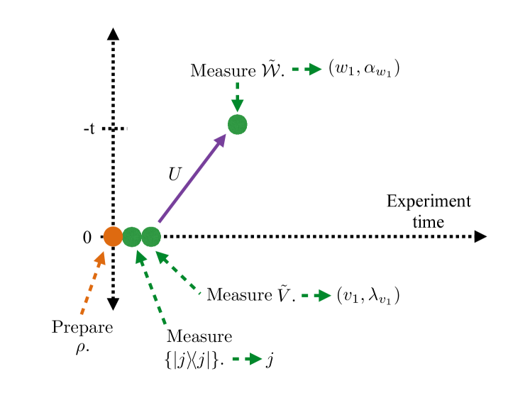
(a)

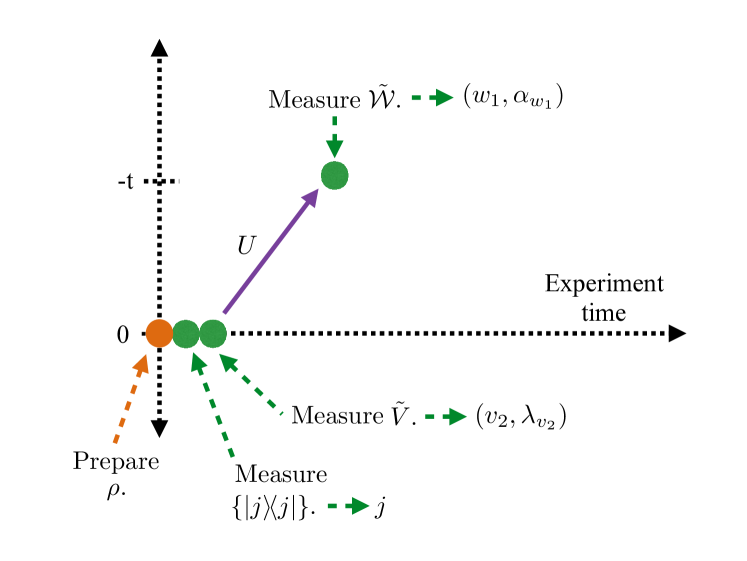
(b)

Figure 18: Quantum processes described by the probability amplitudes $A_{\rho}^{\rm TOC}$ in the time-ordered correlator (TOC) $F_{\rm TOC}(t)$: $F_{\rm TOC}(t)$, like $F(t)$, equals a moment of a summed quasiprobability (Theorem 4). The quasiprobability, $\tilde{A}_{\rho}^{\rm TOC}$, equals a sum of multiplied probability amplitudes $A_{\rho}^{\rm TOC}$ [Eq. (V.4.3)]. Each product contains two factors: $A_{\rho}^{\rm TOC}(j;v_{1},\lambda_{v_{1}};w_{1},\alpha_{w_{1}})$ denotes the probability amplitude associated with the “forward” process in Fig. 18(a). The system, $S$, is prepared in a state $\rho$. The $\rho$ eigenbasis $\left\{\lvert j\rangle\!\langle j\rvert\right\}$ is measured, yielding outcome $j$. $\tilde{V}$ is measured, yielding outcome $(v_{1},\lambda_{v_{1}})$. $S$ is evolved forward in time under the unitary $U$. $\tilde{\mathcal{W}}$ is measured, yielding outcome $(w_{1},\alpha_{w_{1}})$. Along the abscissa runs the time measured by a laboratory clock. Along the ordinate runs the $t$ in $U:=e^{-iHt}$. The second factor in each $\tilde{A}_{\rho}^{\rm TOC}$ product is $A_{\rho}^{\rm TOC}(j;v_{2},\lambda_{v_{2}};w_{1},\alpha_{w_{1}})^{*}$. This factor relates to the process in Fig. 18(b). The operations are those in Fig. 18(a). The processes’ initial measurements yield the same outcome. So do the final measurements. The middle outcomes might differ. Complex-conjugating $A_{\rho}^{\rm TOC}$ yields the probability amplitude associated with the reverse process. Figures 18(a) and 18(b) depict no time reversals. Each analogous OTOC figure (Fig. 2(a) and Fig. 2(b)) depicts two.

$\mathscr{P}_{A}^{\rm TOC}$ results from eliminating, from $\mathscr{P}_{A}$, the initial $U$, $\tilde{\mathcal{W}}$ measurement, and $U^{\dagger}$. $A_{\rho}$ encodes two time reversals. $A_{\rho}^{\rm TOC}$ encodes none, as one might expect.

V.4.3 TOC quasiprobability $\tilde{A}^{\rm TOC}_{\rho}$

Consider a $\mathscr{P}_{A}^{\rm TOC}$ implementation that yields the outcomes $j$, $(v_{2},\lambda_{v_{2}})$, and $(w_{1},\alpha_{w_{1}})$. Such an implementation appears in Fig. 18(b). The first and last outcomes [$j$ and $(w_{1},\alpha_{w_{1}})$] equal those in Fig. 18(a), as in the OTOC case. The middle outcome can differ. This process corresponds to the probability amplitude

$$A_{\rho}^{\rm TOC}(j;v_{2},\lambda_{v_{2}};w_{1},\alpha_{w_{1}})$$

$$\quad=\langle w_{1},\alpha_{w_{1}}|U|v_{2},\lambda_{v_{2}}\rangle\langle v_{2},\lambda_{v_{2}}|j\rangle\>\sqrt{p_{j}}\,.$$ (142)

Complex conjugation reverses the inner products, yielding the reverse process’s amplitude.

We multiply this reverse amplitude by the forward amplitude (V.4.2). Summing over $j$ yields the TOC quasiprobability:

$$\tilde{A}^{\rm TOC}_{\rho}(v_{1},\lambda_{v_{1}};w_{1},\alpha_{w_{1}};v_{2},\lambda_{v_{2}})$$

$$:=\sum_{j}A_{\rho}^{\rm TOC}(j;v_{2},\lambda_{v_{2}};w_{1},\alpha_{w_{1}})^{*}A_{\rho}^{\rm TOC}(j;v_{1},\lambda_{v_{1}};w_{1},\alpha_{w_{1}})$$ (143)

$$=\langle v_{2},\lambda_{v_{2}}|U^{\dagger}|w_{1},\alpha_{w_{1}}\rangle\langle w_{1},\alpha_{w_{1}}|U|v_{1},\lambda_{v_{1}}\rangle$$

$$\qquad\times\langle v_{1},\lambda_{v_{1}}|\rho|v_{2},\lambda_{v_{2}}\rangle\,.$$ (144)

Like $\tilde{A}_{\rho}$, $\tilde{A}^{\rm TOC}_{\rho}$ is an extended Kirkwood-Dirac quasiprobability. $\tilde{A}^{\rm TOC}_{\rho}$ is 2-extended, whereas $\tilde{A}_{\rho}$ is 3-extended. $\tilde{A}^{\rm TOC}_{\rho}$ can be inferred from a weak-measurement protocol $\mathcal{P}^{\rm TOC}$:

1. Prepare $\rho$.

2. Measure $\tilde{V}$ weakly.

3. Evolve the system forward under $U$.

4. Measure $\tilde{\mathcal{W}}$ weakly.

5. Evolve the system backward under $U^{\dagger}$.

6. Measure $\tilde{V}$ strongly.

$\mathcal{P}^{\rm TOC}$ requires just two weak measurements. The weak-measurement protocol $\mathcal{P}$ for inferring $\tilde{A}_{\rho}$ requires three. $\mathcal{P}^{\rm TOC}$ requires one time reversal; $\mathcal{P}$ requires two.

In a simple case, every $A_{\rho}^{\rm TOC}(.)$ value reduces to a probability value. Suppose that $\rho$ shares the $\tilde{V}$ eigenbasis, as in Eq. (35). The $(v_{2},\lambda_{v_{2}})$ in Eq. (V.4.3) comes to equal $(v_{1},\lambda_{v_{1}})$; Figures 18(a) and 18(b) become identical. Equation (V.4.3) reduces to

$$A_{\rho_{V}}^{\rm TOC}(v_{1},\lambda_{v_{1}};w_{1},\alpha_{w_{1}};v_{2},\lambda_{v_{2}})$$ (145)

$$=|\langle w_{1},\alpha_{w_{1}}|U|v_{1},\lambda_{v_{1}}\rangle|^{2}\,p_{v_{1},\lambda_{v_{1}}}\,\delta_{v_{1}v_{2}}\,\delta_{\lambda_{v_{1}}\lambda_{v_{2}}}$$ (146)

$$=p(w_{1},\alpha_{w_{1}}|v_{1},\lambda_{v_{1}})\,p_{v_{1},\lambda_{v_{1}}}\,\delta_{v_{1}v_{2}}\,\delta_{\lambda_{v_{1}}\lambda_{v_{2}}}$$ (147)

$$=p(v_{1},\lambda_{v_{1}};w_{1},\alpha_{w_{1}})\,\delta_{v_{1}v_{2}}\,\delta_{\lambda_{v_{1}}\lambda_{v_{2}}}\,.$$ (148)

The $p(a|b)$ denotes the conditional probability that, if $b$ has occurred, $a$ will occur. $p(a;b)$ denotes the joint probability that $a$ and $b$ will occur.

All values $\tilde{A}_{\rho_{V}}^{\rm TOC}(.)$ of the TOC quasiprobability have reduced to probability values. Not all values of $\tilde{A}_{\rho_{V}}$ reduce: The values associated with $(v_{2},\lambda_{v_{2}})=(v_{1},\lambda_{v_{1}})$ or $(w_{3},\alpha_{w_{3}})=(w_{2},\alpha_{w_{2}})$ reduce to products of probabilities. [See the analysis around Eq. (36).] The OTOC quasiprobability encodes nonclassicality—violations of the axioms of probability—more resilient than the TOC quasiprobability’s.

V.4.4 Complex TOC distribution $P_{\rm TOC}(W_{\rm TOC},W^{\prime}_{\rm TOC})$

Let $W_{\rm TOC}$ and $W^{\prime}_{\rm TOC}$ denote random variables analogous to thermodynamic work. We fix the constraints $W_{\rm TOC}=w_{1}v_{2}$ and $W^{\prime}_{\rm TOC}=w_{1}v_{1}$. ($w_{1}$ and $v_{2}$ need not be complex-conjugated because they are real, as $\mathcal{W}$ and $V$ are Hermitian.) Multiple outcome sextuples $(v_{2},\lambda_{v_{2}};w_{1},\alpha_{w_{1}};v_{1},\lambda_{v_{1}})$ satisfy these constraints. Each sextuple corresponds to a quasiprobability $\tilde{A}^{\rm TOC}_{\rho}(.)$. We sum the quasiprobabilities that satisfy the constraints:

$$P_{\rm TOC}(W_{\rm TOC},W^{\prime}_{\rm TOC}):=\sum_{(v_{1},\lambda_{v_{1}}),(w_{1},\alpha_{w_{1}}),(v_{2},\lambda_{v_{2}})}$$

$$\times\tilde{A}_{\rho}^{\rm TOC}(v_{1},\lambda_{v_{1}};w_{1},\alpha_{w_{1}};v_{2},\lambda_{v_{2}})\,\delta_{W(w_{1}^{*}v_{2}^{*})}\,\delta_{W^{\prime}(w_{1}v_{1})}\,.$$ (149)

$P_{\rm TOC}$ forms a complex distribution. Let $f$ denote any function of $W_{\rm TOC}$ and $W^{\prime}_{\rm TOC}$. The $P_{\rm TOC}$ average of $f$ is

$$\left\langle f(W_{\rm TOC},W^{\prime}_{\rm TOC})\right\rangle$$ (150)

$$:=\sum_{W_{\rm TOC},W^{\prime}_{\rm TOC}}f(W_{\rm TOC},W^{\prime}_{\rm TOC})P_{\rm TOC}(W_{\rm TOC},W^{\prime}_{\rm TOC})\,.$$

V.4.5 TOC as a moment of the complex distribution

The TOC obeys an equality analogous to Eq. (11) in YungerHalpern_17_Jarzynski .

Theorem 4 (Jarzynski-like theorem for the TOC).

The time-ordered correlator (140) equals a moment of the complex distribution (V.4.4):

$$F_{\rm TOC}(t)=\frac{\partial^{2}}{\partial\beta\,\partial\beta^{\prime}}\left\langle e^{-(\beta W_{\rm TOC}+\beta^{\prime}W^{\prime}_{\rm TOC})}\right\rangle\Bigg{\rvert}_{\beta,\beta^{\prime}=0},$$ (151)

wherein $\beta,\beta^{\prime}\in\mathbb{R}$.

Proof.

The proof is analogous to the proof of Theorem 1 in YungerHalpern_17_Jarzynski . ∎

Equation (151) can be recast as $F_{\rm TOC}(t)=\left\langle W_{\rm TOC}W^{\prime}_{\rm TOC}\right\rangle\,,$ along the lines of Eq. (45).

V.5 Higher-order OTOCs as moments of longer (summed) quasiprobabilities

Differentiating a characteristic function again and again yields higher- and higher-point correlation functions. So does differentiating $P(W,W^{\prime})$ again and again. But each resulting correlator encodes just $\mathscr{K}=3$ time reversals. Let $\bar{\mathscr{K}}=\frac{1}{2}(\mathscr{K}+1)=2,3,\ldots$, for $\mathscr{K}=3,5,\ldots$ A $\bar{\mathscr{K}}$-fold OTOC has been defined Roberts_16_Chaos ; Hael_17_Classification :

$$F^{(\bar{\mathscr{K}})}(t):=\langle\underbrace{\mathcal{W}(t)V\ldots\mathcal{W}(t)V}_{2\bar{\mathscr{K}}}\rangle\equiv{\rm Tr}\bm{(}\rho\underbrace{\mathcal{W}(t)V\ldots\mathcal{W}(t)V}_{2\bar{\mathscr{K}}}\bm{)}\,.$$ (152)

Each such correlation function contains $\bar{\mathscr{K}}$ Heisenberg-picture operators $\mathcal{W}(t)$ interleaved with $\bar{\mathscr{K}}$ time-0 operators $V$. $F^{(\bar{\mathscr{K}})}(t)$ encodes $2\bar{\mathscr{K}}-1=\mathscr{K}$ time reversals, illustrated in Fig. 19. We focus on Hermitian $\mathcal{W}$ and $V$, as in Maldacena_15_Bound ; HosurYoshida_16_Chaos , for simplicity.

The conventional OTOC corresponds to $\mathscr{K}=3$ and $\bar{\mathscr{K}}=2$: $F(t)=F^{(2)}(t)$. If $\mathscr{K}<3$, $F^{(\bar{\mathscr{K}})}(t)$ is not OTO.

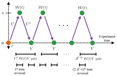
Figure 19: $\bar{\mathscr{K}}$-fold out-of-time-ordered correlator (OTOC): The conventional OTOC [Eq. (28)], encodes just three time reversals. The $\bar{\mathscr{K}}$-fold OTOC $F^{(\bar{\mathscr{K}})}(t)$ encodes $2\bar{\mathscr{K}}-1=\mathscr{K}=3,5,\ldots$ time reversals. The time measured by a laboratory clock runs along the abscissa. The ordinate represents the time parameter $t$, which may be inverted in experiments. The orange, leftmost dot represents the state preparation $\rho$. Each green dot represents a $\mathcal{W}(t)$ or a $V$. Each purple line represents a unitary time evolution. The diagram, scanned from left to right, represents $F^{(\bar{\mathscr{K}})}(t)$, scanned from left to right.

The greater the $\mathscr{K}$, the longer the distribution $P^{(\mathscr{K})}$ of which $F^{(\bar{\mathscr{K}})}(t)$ equals a moment. We define $P^{(\mathscr{K})}$ in three steps: We recall the $\mathscr{K}$-extended quasiprobability $\tilde{A}_{\rho}^{(\mathscr{K})}$ [Eq. (99)]. We introduce measurable random variables $W_{\ell}$ and $W^{\prime}_{\ell^{\prime}}$. These variables participate in constraints on sums of $\tilde{A}_{\rho}^{(\mathscr{K})}(.)$ values.

Let us evaluate Eq. (99) on particular arguments:

$$\tilde{A}_{\rho}^{(\mathscr{K})}(v_{1},\lambda_{v_{1}};w_{2},\alpha_{w_{2}};\ldots;v_{\bar{\mathscr{K}}},\lambda_{v_{\bar{\mathscr{K}}}};w_{\bar{\mathscr{K}}+1},\alpha_{w_{\bar{\mathscr{K}}+1}})$$

$$=\langle w_{\bar{\mathscr{K}}+1},\alpha_{w_{\bar{\mathscr{K}}+1}}|U|v_{\bar{\mathscr{K}}},\lambda_{v_{\bar{\mathscr{K}}}}\rangle\langle v_{\bar{\mathscr{K}}},\lambda_{v_{\bar{\mathscr{K}}}}|U^{\dagger}|w_{\bar{\mathscr{K}}},\alpha_{w_{\bar{\mathscr{K}}}}\rangle$$

$$\times\ldots\times\langle w_{2},\alpha_{w_{2}}|U|v_{1},\lambda_{v_{1}}\rangle\langle v_{1},\lambda_{v_{1}}|\rho U^{\dagger}|w_{\bar{\mathscr{K}}+1},\alpha_{w_{\bar{\mathscr{K}}+1}}\rangle\,.$$ (153)

One can infer $\tilde{A}_{\rho}^{(\mathscr{K})}$ from the interferometry scheme in YungerHalpern_17_Jarzynski and from weak measurements. Upon implementing one batch of the interferometry trials, one can infer $\tilde{A}_{\rho}^{(\mathscr{K})}$ for all $\mathscr{K}$-values: One has measured all the inner products $\langle a|\mathcal{U}|b\rangle$. Multiplying together arbitrarily many inner products yields an arbitrarily high-$\mathscr{K}$ quasiprobability. Having inferred some $\tilde{A}_{\rho}^{(\mathscr{K})}$, one need not perform new experiments to infer $\tilde{A}_{\rho}^{(\mathscr{K}+2)}$. To infer $\tilde{A}_{\rho}^{(\mathscr{K})}$ from weak measurements, one first prepares $\rho$. One performs $\mathscr{K}=2\bar{\mathscr{K}}-1$ weak measurements interspersed with unitaries. (One measures $\tilde{V}$ weakly, evolves with $U$, measures $\tilde{\mathcal{W}}$ weakly, evolves with $U^{\dagger}$, etc.) Finally, one measures $\tilde{\mathcal{W}}$ strongly. The strong measurement corresponds to the anomalous index $\bar{\mathscr{K}}+1$ in $(w_{\bar{\mathscr{K}}+1},\alpha_{w_{\bar{\mathscr{K}}+1}})$.

We define $2\bar{\mathscr{K}}$ random variables

$$W_{\ell}\in\{w_{\ell}\}\qquad\forall\ell=2,3,\ldots,\bar{\mathscr{K}}+1\qquad\text{and}$$ (154)

$$W^{\prime}_{\ell^{\prime}}\in\{v_{\ell^{\prime}}\}\qquad\forall\ell^{\prime}=1,2,\ldots,\bar{\mathscr{K}}\,.$$ (155)

Consider fixing the values of the $W_{\ell}$’s and the $W^{\prime}_{\ell^{\prime}}$’s. Certain quasiprobability values $\tilde{A}_{\rho}^{(\mathscr{K})}(.)$ satisfy the constraints $W_{\ell}=w_{\ell}$ and $W^{\prime}_{\ell^{\prime}}=v_{\ell^{\prime}}$ for all $\ell$ and $\ell^{\prime}$. Summing these quasiprobability values yields

$$P^{(\mathscr{K})}(W_{2},W_{3},\ldots,W_{\bar{\mathscr{K}}+1},W^{\prime}_{1},W^{\prime}_{2},\ldots,W^{\prime}_{\bar{\mathscr{K}}})$$ (156)

$$:=\sum_{W_{2},W_{3},\ldots,W_{\bar{\mathscr{K}}+1}}\sum_{W^{\prime}_{1},W^{\prime}_{2},\ldots,W^{\prime}_{\bar{\mathscr{K}}}}$$

$$\tilde{A}_{\rho}^{(\mathscr{K})}(v_{1},\lambda_{v_{1}};w_{2},\alpha_{w_{2}};\ldots;v_{\bar{\mathscr{K}}},\lambda_{v_{\bar{\mathscr{K}}}};w_{\bar{\mathscr{K}}+1},\alpha_{w_{\bar{\mathscr{K}}+1}})$$

$$\times\left(\delta_{W_{2}w_{2}}\times\ldots\times\delta_{W_{\bar{\mathscr{K}}+1}w_{\bar{\mathscr{K}}+1}}\right)\left(\delta_{W^{\prime}_{1}v_{1}}\times\ldots\times\delta_{W^{\prime}_{\bar{\mathscr{K}}}v_{\bar{\mathscr{K}}}}\right).$$

Theorem 5 (The $\bar{\mathscr{K}}$-fold OTOC as a moment).

The $\bar{\mathscr{K}}$-fold OTOC equals a $2\bar{\mathscr{K}}^{\rm th}$ moment of the complex distribution (156):

$$F^{(\bar{\mathscr{K}})}(t)=\frac{\partial^{2\bar{\mathscr{K}}}}{\partial\beta_{2}\ldots\partial\beta_{\bar{\mathscr{K}}+1}\,\partial\beta^{\prime}_{1}\ldots\partial\beta^{\prime}_{\bar{\mathscr{K}}}}$$

$$\left\langle\exp\left(-\left[\sum_{\ell=2}^{\bar{\mathscr{K}}+1}\beta_{\ell}W_{\ell}+\sum_{\ell^{\prime}=1}^{\bar{\mathscr{K}}}\beta^{\prime}_{\ell^{\prime}}W^{\prime}_{\ell^{\prime}}\right]\right)\right\rangle\Bigg{\lvert}_{\beta_{\ell},\beta^{\prime}_{\ell^{\prime}}=0\;\forall\ell,\ell^{\prime}}\,,$$ (157)

wherein $\beta_{\ell},\beta^{\prime}_{\ell}\in\mathbb{R}$.

Proof.

The proof proceeds in analogy with the proof of Theorem 1 in YungerHalpern_17_Jarzynski . ∎

The greater the $\mathscr{K}$, the “longer” the quasiprobability $\tilde{A}_{\rho}^{(\mathscr{K})}$. The more weak measurements are required to infer $\tilde{A}_{\rho}^{(\mathscr{K})}$. Differentiating $\tilde{A}_{\rho}^{(\mathscr{K})}$ more does not raise the number of time reversals encoded in the correlator.

Equation (5) can be recast as $F^{(\bar{\mathscr{K}})}(t)=\left\langle\left(\prod_{\ell=2}^{\bar{\mathscr{K}}+1}W_{\ell}\right)\left(\prod_{\ell^{\prime}=1}^{\bar{\mathscr{K}}}W^{\prime}_{\ell^{\prime}}\right)\right\rangle\,,$ along the lines of Eq. (45).

VI Outlook

We have characterized the quasiprobability $\tilde{A}_{\rho}$ that “lies behind” the OTOC $F(t)$. $\tilde{A}_{\rho}$, we have argued, is an extension of the Kirkwood-Dirac distribution used in quantum optics. We have analyzed and simplified measurement protocols for $\tilde{A}_{\rho}$, calculated $\tilde{A}_{\rho}$ numerically and on average over Brownian circuits, and investigated mathematical properties. This work redounds upon quantum chaos, quasiprobability theory, and weak-measurement physics. As the OTOC equals a combination of $\tilde{A}_{\rho}(.)$ values, $\tilde{A}_{\rho}$ provides more-fundamental information about scrambling. The OTOC motivates generalizations of, and fundamental questions about, KD theory. The OTOC also suggests a new application of sequential weak measurements.

At this intersection of fields lie many opportunities. We classify the opportunities by the tools that inspired them: experiments, calculations, and abstract theory.

VI.1 Experimental opportunities

We expect the weak-measurement scheme for $\tilde{A}_{\rho}$ and $F(t)$ to be realizable in the immediate future. Candidate platforms include superconducting qubits, trapped ions, ultracold atoms, and perhaps NMR. Experimentalists have developed key tools required to implement the protocol Bollen_10_Direct ; Lundeen_11_Direct ; Lundeen_12_Procedure ; Bamber_14_Observing ; Mirhosseini_14_Compressive ; White_16_Preserving ; Hacohen_16_Quantum ; Browaeys_16_Experimental ; Piacentini_16_Measuring ; Suzuki_16_Observation ; Thekkadath_16_Direct .

Achievable control and dissipation must be compared with the conditions needed to infer the OTOC. Errors might be mitigated with tools under investigation Swingle_Resilience .

VI.2 Opportunities motivated by calculations

Numerical simulations and analytical calculations point to three opportunities.

Physical models’ OTOC quasiprobabilities may be evaluated. The Sachdev-Ye-Kitaev model, for example, scrambles quickly Sachdev_93_Gapless ; Kitaev_15_Simple . The quasiprobability’s functional form may suggest new insights into chaos. Our Brownian-circuit calculation (Sec. IV), while a first step, involves averages over unitaries. Summing quasiprobabilities can cause interference to dampen nonclassical behaviors Dressel_15_Weak . Additionally, while unitary averages model chaotic evolution, explicit Hamiltonian evolution might provide different insights. Explicit Hamiltonian evolution would also preclude the need to calculate higher moments of the quasiprobability.

In some numerical plots, the real part $\Re(\tilde{\mathscr{A}}_{\rho})$ bifurcates. These bifurcations resemble classical-chaos pitchforks Strogatz_00_Non . Classical-chaos plots bifurcate when a differential equation’s equilibrium point branches into three. The OTOC quasiprobability $\tilde{A}_{\rho}$ might be recast in terms of equilibria. Such a recasting would strengthen the parallel between classical chaos and the OTOC.

Finally, the Brownian-circuit calculation has untied threads. We calculated only the first moment of $\tilde{\mathscr{A}}_{\rho}$. Higher moments may encode physics less visible in $F(t)$. Also, evaluating certain components of $\tilde{\mathscr{A}}_{\rho}$ requires new calculational tools. These tools merit development, then application to $\tilde{\mathscr{A}}_{\rho}$. An example opportunity is discussed after Eq. (90).

VI.3 Fundamental-theory opportunities

Seven opportunities concern the mathematical properties and physical interpretations of $\tilde{A}_{\rho}$.

The KD quasiprobability prompts the question, “Is the OTOC definition of ‘maximal noncommutation’ consistent with the mutually-unbiased-bases definition?” Recall Sec. V.3: We decomposed an operator $\rho^{\prime}$ in terms of a set $\mathcal{S}=\left\{\frac{\lvert a\rangle\!\langle f\rvert}{\langle f|a\rangle}\right\}_{\langle f|a\rangle\neq 0}$ of operators. In the KD-quasiprobability literature, the bases $\mathcal{S}_{a}=\left\{\lvert a\rangle\right\}$ and $\mathcal{S}_{f}=\left\{\lvert f\rangle\right\}$ tend to be mutually unbiased (MU): $|\langle f|a\rangle|=\frac{1}{\sqrt{d}}\;\forall a,f$. Let $\mathcal{A}$ and $\mathcal{B}$ denote operators that have MU eigenbases. Substituting $\mathcal{A}$ and $\mathcal{B}$ into an uncertainty relation maximizes the lower bound on an uncertainty Coles_15_Entropic . In this quantum-information (QI) sense, $\mathcal{A}$ and $\mathcal{B}$ noncommute maximally.

In Sec. V.3, $\mathcal{S}_{a}=\left\{\lvert v_{2},\lambda_{v_{2}}\rangle\right\}$, and $\mathcal{S}_{f}=\left\{U^{\dagger}\lvert w_{3},\alpha_{w_{3}}\rangle\right\}$. These $\mathcal{S}$’s are eigenbases of $V$ and $\mathcal{W}(t)$. When do we expect these eigenbases to be MU, as in the KD-quasiprobability literature? After the scrambling time $t_{*}$—after $F(t)$ decays to zero—when $\mathcal{W}(t)$ and $V$ noncommute maximally in the OTOC sense.

The OTOC provides one definition of “maximal noncommutation.” MUBs provide a QI definition. To what extent do these definitions overlap? Initial results show that, in some cases, the distribution over possible values of $|\langle v_{2},\lambda_{v_{2}}|U|w_{3},\alpha_{w_{3}}\rangle|$ peaks at $\frac{1}{\sqrt{d}}$. But the distribution approaches this form before $t_{*}$. Also, the distribution’s width seems constant in $d$. Further study is required. The overlap between OTOC and two QI definitions of scrambling have been explored already: (1) When the OTOC is small, a tripartite information is negative HosurYoshida_16_Chaos . (2) An OTOC-like function is proportional to a frame potential that quantifies pseudorandomness Roberts_16_Chaos . The relationship between the OTOC and a third QI sense of incompatibility—MUBs and entropic uncertainty relations—merits investigation.

Second, $\tilde{A}_{\rho}$ effectively has four arguments, apart from $\rho$ (Sec. V.1). The KD quasiprobability has two. This doubling of indices parallels the Choi-Jamiolkowski (CJ) representation of quantum channels Preskill_15_Ch3 . Hosur et al. have, using the CJ representation, linked $F(t)$ to the tripartite information HosurYoshida_16_Chaos . The extended KD distribution might be linked to information-theoretic quantities similarly.

Third, our $P(W,W^{\prime})$ and weak-measurement protocol resemble analogs in Solinas_15_Full ; Solinas_16_Probing . {See Alonso_16_Thermodynamics ; Miller_16_Time ; Elouard_17_Role for frameworks similar to Solinas and Gasparinetti’s (S&G’s).} Yet Solinas_15_Full ; Solinas_16_Probing concern quantum thermodynamics, not the OTOC. The similarity between the quasiprobabilities in Solinas_15_Full ; Solinas_16_Probing and those in YungerHalpern_17_Jarzynski , their weak-measurement protocol and ours, and the thermodynamic agendas in Solinas_15_Full ; Solinas_16_Probing and YungerHalpern_17_Jarzynski suggest a connection between the projects Jordan_chat ; Solinas_chat . The connection merits investigation and might yield new insights. For instance, S&G calculate the heat dissipated by an open quantum system that absorbs work (Solinas_15_Full, , Sec. IV). OTOC theory focuses on closed systems. Yet experimental systems are open. Dissipation endangers measurements of $F(t)$. Solinas and Gasparinetti’s toolkit might facilitate predictions about, and expose interesting physics in, open-system OTOCs.

Fourth, $W$ and $W^{\prime}$ suggest understudies for work in quantum thermodynamics. Thermodynamics sprouted during the 1800s, alongside steam engines and factories. How much work a system could output—how much “orderly” energy one could reliably draw—held practical importance. Today’s experimentalists draw energy from power plants. Quantifying work may be less critical than it was 150 years ago. What can replace work in the today’s growing incarnation of thermodynamics, quantum thermodynamics? Coherence relative to the energy eigenbasis is being quantified Lostaglio_15_Description ; Narasimhachar_15_Low . The OTOC suggests alternatives: $W$ and $W^{\prime}$ are random variables, analogous to work, natural to quantum-information scrambling. The potential roles of $W$ and $W^{\prime}$ within quantum thermodynamics merit exploration.

Fifth, relationships amongst three ideas were identified recently:

1. We have linked quasiprobabilities with the OTOC, following YungerHalpern_17_Jarzynski .

2. Aleiner et al. Aleiner_16_Microscopic and Haehl et al. Haehl_16_Schwinger_I ; Haehl_16_Schwinger_II have linked the OTOC with Schwinger-Keldysh path integrals.

3. Hofer has linked Schwinger-Keldysh path integrals with quasiprobabilities Hofer_17_Quasi .

The three ideas—quasiprobabilities, the OTOC, and Schwinger-Keldysh path integrals—form the nodes of the triangle in Fig. 20. The triangle’s legs were discovered recently; their joinings can be probed further. For example, Hofer focuses on single-timefold path integrals. OTOC path integrals contain multiple timefolds Aleiner_16_Microscopic ; Haehl_16_Schwinger_I ; Haehl_16_Schwinger_II . Just as Hofer’s quasiprobabilities involve fewer timefolds than the OTOC quasiprobability $\tilde{A}_{\rho}$, the TOC quasiprobability $\tilde{A}^{\rm TOC}_{\rho}$ (V.4.3) can be inferred from fewer weak measurements than $\tilde{A}_{\rho}$ can. One might expect Hofer’s quasiprobabilities to relate to $\tilde{A}^{\rm TOC}_{\rho}$. Kindred works, linking quasiprobabilities with out-of-time ordering, include Manko_00_Lyapunov ; Bednorz_13_Nonsymmetrized ; Oehri_16_Time ; Hofer_17_Quasi ; Lee_17_On .

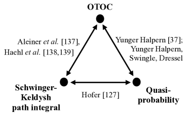
Figure 20: Three interrelated ideas: Relationships amongst the out-of-time-ordered correlator, quasiprobabilities, and Schwinger-Keldysh path integrals were articulated recently.

Sixth, the OTOC equals a moment of the complex distribution $P(W,W^{\prime})$ YungerHalpern_17_Jarzynski . The OTOC has been bounded with general-relativity and Lieb-Robinson tools Maldacena_15_Bound ; Lashkari_13_Towards . A more information-theoretic bound might follow from the Jarzynski-like equality in YungerHalpern_17_Jarzynski .

Finally, the KD distribution consists of the coefficients in a decomposition of a quantum state $\rho\in\mathcal{D}(\mathcal{H})$ Lundeen_11_Direct ; Lundeen_12_Procedure (Sec. I.1.3). $\rho$ is decomposed in terms of a set $\mathcal{S}:=\left\{\frac{\lvert a\rangle\!\langle f\rvert}{\langle f|a\rangle}\right\}$ of operators. $\mathcal{S}$ forms a basis for $\mathcal{H}$ only if $\langle f|a\rangle\neq 0\;\forall a,f$. The inner product has been nonzero in experiments, because $\left\{\lvert a\rangle\right\}$ and $\left\{\lvert f\rangle\right\}$ are chosen to be mutually unbiased bases (MUBs): They are eigenbases of “maximally noncommuting” observables. The OTOC, evaluated before the scrambling time $t=t_{*}$, motivates a generalization beyond MUBs. What if, $F(t)$ prompts us to ask, $\langle f|a\rangle=0$ for some $a,f$ (Sec. V.3)? The decomposition comes to be of an “asymmetrically decohered” $\rho^{\prime}$. This decoherence’s physical significance merits investigation. The asymmetry appears related to time irreversibility. Tools from non-Hermitian quantum mechanics might offer insight Moiseyev_11_Non .

Appendix A Mathematical properties of $P(W,W^{\prime})$

Summing $\tilde{A}_{\rho}$, with constraints, yields $P(W,W^{\prime})$ [Eq. (37)]. Hence properties of $\tilde{A}_{\rho}$ (Sec. V.1) imply properties of $P(W,W^{\prime})$.

Property 8.

$P(W,W^{\prime})$ is a map from a composition of two sets of complex numbers to the complex numbers: $P\>:\>\left\{W\right\}\times\left\{W^{\prime}\right\}\to\mathbb{C}$. The range is not necessarily real: $\mathbb{C}\supset\mathbb{R}$.

Summing quasiprobability values can eliminate nonclassical behavior: Interference can reduce quasiprobabilities’ nonreality and negativity. Property 6 consists of an example. One might expect $P(W,W^{\prime})$, a sum of $\tilde{A}_{\rho}(.)$ values, to be real. Yet $P(W,W^{\prime})$ is nonreal in many numerical simulations (Sec. III).

Property 9.

Marginalizing $P(W,W^{\prime})$ over one argument yields a probability if $\rho$ shares the $\tilde{V}$ eigenbasis or the $\tilde{\mathcal{W}}(t)$ eigenbasis.

Consider marginalizing Eq. (37) over $W^{\prime}$. The $(w_{2},\alpha_{w_{2}})$ and $(v_{1},\lambda_{v_{1}})$ sums can be performed explicitly:

$$P(W) :=\sum_{W^{\prime}}P(W,W^{\prime})$$ (A1)

$$=\sum_{\begin{subarray}{c}(v_{2},\lambda_{v_{2}}),\\ (w_{3},\alpha_{w_{3}})\end{subarray}}\langle w_{3},\alpha_{w_{3}}|U|v_{2},\lambda_{v_{2}}\rangle\langle v_{2},\lambda_{v_{2}}|\rho U^{\dagger}|w_{3},\alpha_{w_{3}}\rangle$$

$$\qquad\qquad\qquad\times\delta_{W(w_{3}^{*}v_{2}^{*})}\,.$$ (A2)

The final expression is not obviously a probability.

But suppose that $\rho$ shares its eigenbasis with $\tilde{V}$ or with $\tilde{\mathcal{W}}(t)$. Suppose, for example, that $\rho$ has the form in Eq. (35). Equation (A) simplifies:

$$P(W) =\sum_{\begin{subarray}{c}(v_{2},\lambda_{v_{2}}),\\ (w_{3},\alpha_{w_{3}})\end{subarray}}p(v_{2},\lambda_{v_{2}};w_{3},\alpha_{w_{3}})\,\delta_{W(w_{3}^{*}v_{2}^{*})}\,.$$ (A3)

The $p(v_{2},\lambda_{v_{2}};w_{3},\alpha_{w_{3}}):=|\langle w_{3},\alpha_{w_{3}}|U|v_{2},\lambda_{v_{2}}\rangle|^{2}\,p_{v_{2},\lambda_{v_{2}}}$ denotes the joint probability that a $\tilde{V}$ measurement of $\rho$ yields $(v_{2},\lambda_{v_{2}})$ and, after a subsequent evolution under $U$, a $\tilde{\mathcal{W}}$ measurement yields $(w_{3},\alpha_{w_{3}})$.

Every factor in Eq. (A3) is nonnegative. Summing over $W$ yields a sum over the arguments of $\tilde{A}_{\rho}(.)$. The latter sum equals one, by Property 6: $\sum_{W}P(W)=1$. Hence $P(W)\in[0,1]$. Hence $P(W)$ behaves as a probability.

We can generalize Property 9 to arbitrary Gibbs states $\rho=e^{-H/T}/Z$, using the regulated quasiprobability (110). The regulated OTOC (108) equals a moment of the complex distribution

$$P_{\rm reg}(W,W^{\prime}):=\sum_{\begin{subarray}{c}(v_{1},\lambda_{v_{1}}),(w_{2},\alpha_{w_{2}}),(v_{2},\lambda_{v_{2}})(w_{3},\alpha_{w_{3}})\end{subarray}}$$ (A4)

$$\tilde{A}_{\rho}^{\rm reg}(v_{1},\lambda_{v_{1}};w_{2},\alpha_{w_{2}};v_{2},\lambda_{v_{2}};w_{3},\alpha_{w_{3}})\,\delta_{W(w_{3}^{*}v_{2}^{*})}\,\delta_{W^{\prime}(w_{2}v_{1})}\,.$$

The proof is analogous to the proof of Theorem 1 in YungerHalpern_17_Jarzynski .

Summing over $W^{\prime}$ yields $P_{\rm reg}(W):=\sum_{W^{\prime}}P_{\rm reg}(W,W^{\prime})$. We substitute in from Eq. (A4), then for $\tilde{A}_{\rho}^{\rm reg}$ from Eq. (110). We perform the sum over $W^{\prime}$ explicitly, then the sums over $(w_{2},\alpha_{w_{2}})$ and $(v_{1},\lambda_{v_{1}})$:

$$P_{\rm reg}(W)=\sum_{\begin{subarray}{c}(v_{2},\lambda_{v_{2}})\\ (w_{3},\alpha_{w_{3}})\end{subarray}}|\langle w_{3},\alpha_{w_{3}}|\tilde{U}|v_{2},\lambda_{v_{2}}\rangle|^{2}\,\delta_{W(w_{3}^{*}v_{2}^{*})}\,.$$ (A5)

This expression is real and nonnegative. $P_{\rm reg}(W)$ sums to one, as $P(W)$ does. Hence $P_{\rm reg}(W)\in[0,\,1]$ acts as a probability.

Property 10 (Degeneracy of every $P(W,W^{\prime})$ associated with $\rho=\mathbbm{1}/d$ and with eigenvalue-$(\pm 1)$ operators $\mathcal{W}$ and $V$).

Let the eigenvalues of $\mathcal{W}$ and $V$ be $\pm 1$. For example, let $\mathcal{W}$ and $V$ be Pauli operators. Let $\rho=\mathbbm{1}/d$ be the infinite-temperature Gibbs state. The complex distribution has the degeneracy $P(1,-1)=P(-1,1)$.

Property 10 follows from (1) Eq. (52) and (2) Property 7 of $\tilde{A}_{(\mathbbm{1}/d)}$. Item (2) can be replaced with the trace’s cyclicality. We reason as follows: $P(W,W^{\prime})$ is defined in Eq. (37). Performing the sums over the degeneracies yields $\tilde{\mathscr{A}}_{(\mathbbm{1}/d)}$. Substituting in from Eq. (52) yields

$$P(W,W^{\prime}) =\frac{1}{d}\sum_{v_{1},w_{2},v_{2},w_{3}}{\rm Tr}\left(\Pi^{\mathcal{W}(t)}_{w_{3}}\Pi^{V}_{v_{2}}\Pi^{\mathcal{W}(t)}_{w_{2}}\Pi^{V}_{v_{1}}\right)$$

$$\qquad\qquad\qquad\;\times\delta_{W(w_{3}^{*}v_{2}^{*})}\delta_{W^{\prime}(w_{2}v_{1})}\,.$$ (A6)

Consider inferring $\tilde{A}_{(\mathbbm{1}/d)}$ or $\tilde{\mathscr{A}}_{(\mathbbm{1}/d)}$ from weak measurements. From one trial, we infer about four random variables: $v_{1},w_{2},v_{2}$ and $w_{3}$. Each variable equals $\pm 1$. The quadruple $(v_{1},w_{2},v_{2},w_{3})$ therefore assumes one of sixteen possible values. These four “base” variables are multiplied to form the composite variables $W$ and $W^{\prime}$. The tuple $(W,W^{\prime})$ assumes one of four possible values. Every $(W,W^{\prime})$ value can be formed from each of four values of $(v_{1},w_{2},v_{2},w_{3})$. Table 2 lists the tuple-quadruple correspondences.

$(W,W^{\prime})$	$(v_{1},w_{2},v_{2},w_{3})$
$(1,1)$	$(1,1,1,1),(1,1,-1,-1),(-1,-1,1,1),(-1,-1,-1,-1)$
$(1,-1)$	$(-1,1,1,1),(-1,1,-1,-1),(1,-1,1,1),(1,-1,-1,-1)$
$(-1,1)$	$(1,1,-1,1),(1,1,1,-1),(-1,-1,-1,1),(-1,-1,1,-1)$
$(-1,-1)$	$(-1,1,-1,1),(-1,1,1,-1),(1,-1,-1,1),(1,-1,1,-1)$

Table 2: Correspondence between tuples of composite variables and quadruples of “base” variables: From each weak-measurement trial, one learns about a quadruple $(v_{1},w_{2},v_{2},w_{3})$. Suppose that the out-of-time-ordered-correlator operators $\mathcal{W}$ and $V$ have the eigenvalues $w_{\ell},v_{m}=\pm 1$. For example, suppose that $\mathcal{W}$ and $V$ are Pauli operators. The quadruple’s elements are combined into $W:=w_{3}^{*}v_{2}^{*}$ and $W^{\prime}:=w_{2}v_{1}$. Each $(W,W^{\prime})$ tuple can be formed from each of four quadruples.

Consider any quadruple associated with $(W,W^{\prime})=(1,-1)$, e.g., $(-1,1,1,1)$. Consider swapping $w_{2}$ with $w_{3}$ and swapping $v_{1}$ with $v_{2}$. The result, e.g., $(1,1,-1,1)$, leads to $(W,W^{\prime})=(-1,1)$. This double swap amounts to a cyclic permutation of the quadruple’s elements. This permutation is equivalent to a cyclic permutation of the argument of the (A) trace. This permutation preserves the trace’s value while transforming the trace into $P(-1,1)$. The trace originally equaled $P(1,-1)$. Hence $P(1,-1)=P(-1,1)$.

Appendix B Retrodiction about the symmetrized composite observable $\tilde{\Gamma}:=i(\mathcal{K}\ldots\mathcal{A}-\mathcal{A}\ldots\mathcal{K})$

Section V.2 concerns retrodiction about the symmetrized observable $\Gamma:=\mathcal{K}\ldots\mathcal{A}+\mathcal{A}\ldots\mathcal{K}$. The product $\mathcal{K}\ldots\mathcal{A}$ is symmetrized also in $\tilde{\Gamma}:=i(\mathcal{K}\ldots\mathcal{A}-\mathcal{A}\ldots\mathcal{K})$. One can retrodict about $\tilde{\Gamma}$, using $\mathscr{K}$-extended KD quasiprobabilities $\tilde{A}_{\rho}^{(\mathscr{K})}$, similarly to in Theorem 1.

The value most reasonably attributable retrodictively to the time-$t^{\prime}$ value of $\tilde{\Gamma}$ is given by Eqs. (1), (112), and (114). The conditional quasiprobabilities on the right-hand sides of Eqs. (113) and (115) become

$$\tilde{p}_{\rightarrow}(a,\ldots,k,f|\rho)=\frac{-\Im(\langle f^{\prime}|k\rangle\langle k|\ldots|a\rangle\langle a|\rho^{\prime}|f^{\prime}\rangle)}{\langle f^{\prime}|\rho^{\prime}|f^{\prime}\rangle}$$ (B1)

and

$$\tilde{p}_{\leftarrow}(k,\ldots,a,f|\rho)=\frac{\Im(\langle f^{\prime}|a\rangle\langle a|\ldots|k\rangle\langle k|\rho^{\prime}|f^{\prime}\rangle)}{\langle f^{\prime}|\rho^{\prime}|f^{\prime}\rangle}\,.$$ (B2)

The extended KD distributions become

$$\tilde{A}_{\rho,\rightarrow}^{(\mathscr{K})}(\rho,a,\ldots,k,f)=i\langle f^{\prime}|k\rangle\langle k|\ldots|a\rangle\langle a|\rho^{\prime}|f^{\prime}\rangle$$ (B3)

and

$$\tilde{A}_{\rho,\leftarrow}^{(\mathscr{K})}(\rho,k,\ldots,a,f)=-i\langle f^{\prime}|a\rangle\langle a|\ldots|k\rangle\langle k|\rho|f^{\prime}\rangle\,.$$ (B4)

To prove this claim, we repeat the proof of Theorem 1 until reaching Eq. (122). The definition of $\tilde{\Gamma}$ requires that an $i$ enter the argument of the first $\Re$ and that a $-i$ enter the argument of the second $\Re$. The identity $\Re(iz)=-\Im(z)$, for $z\in\mathbb{C}$, implies Eqs. (B1)–(B4).

References

- (1) S. H. Shenker and D. Stanford, Journal of High Energy Physics 3, 67 (2014).
- (2) S. H. Shenker and D. Stanford, Journal of High Energy Physics 12, 46 (2014).
- (3) S. H. Shenker and D. Stanford, Journal of High Energy Physics 5, 132 (2015).
- (4) D. A. Roberts, D. Stanford, and L. Susskind, Journal of High Energy Physics 3, 51 (2015).
- (5) D. A. Roberts and D. Stanford, Physical Review Letters 115, 131603 (2015).
- (6) J. Maldacena, S. H. Shenker, and D. Stanford, ArXiv e-prints (2015), 1503.01409.
- (7) H. J. Carmichael, Statistical Methods in Quantum Optics I: Master Equations and Fokker-Planck Equations (Springer-Verlag, 2002).
- (8) J. G. Kirkwood, Physical Review 44, 31 (1933).
- (9) P. A. M. Dirac, Rev. Mod. Phys. 17, 195 (1945).
- (10) J. S. Lundeen, B. Sutherland, A. Patel, C. Stewart, and C. Bamber, Nature 474, 188 (2011).
- (11) J. S. Lundeen and C. Bamber, Phys. Rev. Lett. 108, 070402 (2012).
- (12) C. Bamber and J. S. Lundeen, Phys. Rev. Lett. 112, 070405 (2014).
- (13) M. Mirhosseini, O. S. Magaña Loaiza, S. M. Hashemi Rafsanjani, and R. W. Boyd, Phys. Rev. Lett. 113, 090402 (2014).
- (14) J. Dressel, Phys. Rev. A 91, 032116 (2015).
- (15) R. W. Spekkens, Phys. Rev. Lett. 101, 020401 (2008).
- (16) C. Ferrie, Reports on Progress in Physics 74, 116001 (2011).
- (17) A. G. Kofman, S. Ashhab, and F. Nori, Physics Reports 520, 43 (2012).
- (18) J. Dressel, M. Malik, F. M. Miatto, A. N. Jordan, and R. W. Boyd, Rev. Mod. Phys. 86, 307 (2014).
- (19) M. Howard, J. Wallman, V. Veitch, and J. Emerson, Nature 510, 351 (2014).
- (20) N. Delfosse, P. Allard Guerin, J. Bian, and R. Raussendorf, Phys. Rev. X 5, 021003 (2015).
- (21) J. Maldacena, International Journal of Theoretical Physics 38, 1113 (1999).
- (22) E. Witten, Advances in Theoretical and Mathematical Physics 2, 253 (1998).
- (23) S. S. Gubser, I. R. Klebanov, and A. M. Polyakov, Physics Letters B 428, 105 (1998), hep-th/9802109.
- (24) D. Stanford, Journal of High Energy Physics 10, 9 (2016), 1512.07687.
- (25) A. A. Patel and S. Sachdev, ArXiv e-prints (2016), 1611.00003.
- (26) D. Chowdhury and B. Swingle, ArXiv e-prints (2017), 1703.02545.
- (27) A. A. Patel, D. Chowdhury, S. Sachdev, and B. Swingle, ArXiv e-prints (2017), 1703.07353.
- (28) P. Hosur, X.-L. Qi, D. A. Roberts, and B. Yoshida, Journal of High Energy Physics 2, 4 (2016), 1511.04021.
- (29) S. Sachdev and J. Ye, Phys. Rev. Lett. 70, 3339 (1993).
- (30) A. Kitaev, A simple model of quantum holography, KITP strings seminar and Entanglement 2015 program, 2015.
- (31) V. Bollen, Y. M. Sua, and K. F. Lee, Phys. Rev. A 81, 063826 (2010).
- (32) Y. Suzuki, M. Iinuma, and H. F. Hofmann, New Journal of Physics 18, 103045 (2016).
- (33) F. Piacentini et al., Phys. Rev. Lett. 117, 170402 (2016).
- (34) G. S. Thekkadath et al., Phys. Rev. Lett. 117, 120401 (2016).
- (35) T. C. White et al., npj Quantum Information 2, 15022 (2016).
- (36) J. P. Groen et al., Phys. Rev. Lett. 111, 090506 (2013).
- (37) N. Yunger Halpern, Phys. Rev. A 95, 012120 (2017).
- (38) C. Jarzynski, Physical Review Letters 78, 2690 (1997).
- (39) M. Campisi and J. Goold, ArXiv e-prints (2016), 1609.05848.
- (40) N. Tsuji, T. Shitara, and M. Ueda, ArXiv e-prints (2016), 1612.08781.
- (41) B. Swingle, G. Bentsen, M. Schleier-Smith, and P. Hayden, Phys. Rev. A 94, 040302 (2016).
- (42) N. Y. Yao et al., ArXiv e-prints (2016), 1607.01801.
- (43) A. Bohrdt, C. B. Mendl, M. Endres, and M. Knap, ArXiv e-prints (2016), 1612.02434.
- (44) G. Zhu, M. Hafezi, and T. Grover, ArXiv e-prints (2016), 1607.00079.
- (45) I. Danshita, M. Hanada, and M. Tezuka, ArXiv e-prints (2016), 1606.02454.
- (46) N. Tsuji, P. Werner, and M. Ueda, Phys. Rev. A 95, 011601 (2017), 1610.01251.
- (47) J. Li et al., ArXiv e-prints (2016), 1609.01246.
- (48) M. Gärttner et al., ArXiv e-prints (2016), 1608.08938.
- (49) K. X. Wei, C. Ramanathan, and P. Cappellaro, ArXiv e-prints (2016), 1612.05249.
- (50) S. Hacohen-Gourgy et al., Nature 538, 491 (2016).
- (51) R. P. Rundle, T. Tilma, J. H. Samson, and M. J. Everitt, ArXiv e-prints (2016), 1605.08922.
- (52) M. Takita et al., Phys. Rev. Lett. 117, 210505 (2016).
- (53) J. Kelly et al., Nature 519, 66 (2015).
- (54) R. W. Heeres et al., ArXiv e-prints (2016), 1608.02430.
- (55) D. Ristè et al., Nature Communications 6, 6983 (2015).
- (56) S. A. Gardiner, J. I. Cirac, and P. Zoller, Phys. Rev. Lett. 79, 4790 (1997).
- (57) S. K. Choudhary, T. Konrad, and H. Uys, Phys. Rev. A 87, 012131 (2013).
- (58) L. G. Lutterbach and L. Davidovich, Phys. Rev. Lett. 78, 2547 (1997).
- (59) S. Debnath et al., Nature 536, 63 (2016).
- (60) T. Monz et al., Science 351, 1068 (2016).
- (61) N. M. Linke et al., ArXiv e-prints (2016), 1611.06946.
- (62) N. M. Linke et al., ArXiv e-prints (2017), 1702.01852.
- (63) A. Browaeys, D. Barredo, and T. Lahaye, Journal of Physics B: Atomic, Molecular and Optical Physics 49, 152001 (2016).
- (64) C. Guerlin et al., Nature 448, 889 (2007), 0707.3880.
- (65) K. W. Murch, S. J. Weber, C. Macklin, and I. Siddiqi, Nature 502, 211 (2013).
- (66) L. Xiao and J. A. Jones, Physics Letters A 359, 424 (2006).
- (67) D. Lu, A. Brodutch, J. Li, H. Li, and R. Laflamme, New Journal of Physics 16, 053015 (2014).
- (68) W. Brown and O. Fawzi, ArXiv e-prints (2012), 1210.6644.
- (69) P. Hayden and J. Preskill, Journal of High Energy Physics 2007, 120 (2007).
- (70) Y. Sekino and L. Susskind, Journal of High Energy Physics 2008, 065 (2008).
- (71) N. Lashkari, D. Stanford, M. Hastings, T. Osborne, and P. Hayden, Journal of High Energy Physics 2013, 22 (2013).
- (72) Y. Aharonov, D. Z. Albert, and L. Vaidman, Phys. Rev. Lett. 60, 1351 (1988).
- (73) L. M. Johansen, Phys. Lett. A 329, 184 (2004).
- (74) M. J. W. Hall, Phys. Rev. A 64, 052103 (2001).
- (75) M. J. W. Hall, Phys. Rev. A 69, 052113 (2004).
- (76) L. D. Landau and E. M. Lifshitz, Statistical Physics (Pergamon Press, Oxford, England, 1980).
- (77) J. Banerji, Contemporary Physics 48, 157 (2007).
- (78) A. Rihaczek, IEEE Transactions on Information Theory 14, 369 (1968).
- (79) L. Cohen, Proceedings of the IEEE 77, 941 (1989).
- (80) N. W. M. Ritchie, J. G. Story, and R. G. Hulet, Phys. Rev. Lett. 66, 1107 (1991).
- (81) G. J. Pryde, J. L. O’Brien, A. G. White, T. C. Ralph, and H. M. Wiseman, Phys. Rev. Lett. 94, 220405 (2005).
- (82) J. Dressel, C. J. Broadbent, J. C. Howell, and A. N. Jordan, Phys. Rev. Lett. 106, 040402 (2011).
- (83) M. F. Pusey, Phys. Rev. Lett. 113, 200401 (2014).
- (84) M. Waegell et al., ArXiv e-prints (2016), 1609.06046.
- (85) C. Ferrie and J. Combes, Phys. Rev. Lett. 113, 120404 (2014).
- (86) L. Vaidman, ArXiv e-prints (2014), 1409.5386.
- (87) E. Cohen, ArXiv e-prints (2014), 1409.8555.
- (88) Y. Aharonov and D. Rohrlich, ArXiv e-prints (2014), 1410.0381.
- (89) D. Sokolovski, ArXiv e-prints (2014), 1410.0570.
- (90) A. Brodutch, Phys. Rev. Lett. 114, 118901 (2015).
- (91) C. Ferrie and J. Combes, Phys. Rev. Lett. 114, 118902 (2015).
- (92) Y. P. Terletsky, JETP 7, 1290 (1937).
- (93) H. Margenau and R. N. Hill, Prog. Theor. Phys. 26, 722 (1961).
- (94) L. M. Johansen and A. Luis, Phys. Rev. A 70, 052115 (2004).
- (95) H. M. Wiseman, Phys. Rev. A 65, 032111 (2002).
- (96) A. J. Leggett and A. Garg, Phys. Rev. Lett. 54, 857 (1985).
- (97) C. Emary, N. Lambert, and F. Nori, Reports on Progress in Physics 77, 016001 (2014).
- (98) H. F. Hofmann, New Journal of Physics 14, 043031 (2012).
- (99) J. Dressel and A. N. Jordan, Phys. Rev. A 85, 012107 (2012).
- (100) H. F. Hofmann, Phys. Rev. A 89, 042115 (2014).
- (101) H. F. Hofmann, New Journal of Physics 16, 063056 (2014).
- (102) J. Z. Salvail et al., Nat Photon 7, 316 (2013).
- (103) M. Malik et al., Nat Commun 5 (2014), Article.
- (104) G. A. Howland, D. J. Lum, and J. C. Howell, Opt. Express 22, 18870 (2014).
- (105) H. Tasaki, arXiv e-print (2000), cond-mat/0009244.
- (106) J. Cotler, private communication, 2016.
- (107) P. Solinas, private communication, 2016.
- (108) P. Solinas and S. Gasparinetti, Phys. Rev. E 92, 042150 (2015).
- (109) P. Solinas and S. Gasparinetti, Phys. Rev. A 94, 052103 (2016).
- (110) J. J. Alonso, E. Lutz, and A. Romito, Phys. Rev. Lett. 116, 080403 (2016).
- (111) H. J. D. Miller and J. Anders, ArXiv e-prints (2016), 1610.04285.
- (112) C. Elouard, D. A. Herrera-Martí, M. Clusel, and A. Auffèves, npj Quantum Information 3, 9 (2017).
- (113) M. A. Nielsen and I. L. Chuang, Quantum Computation and Quantum Information (Cambridge University Press, 2010).
- (114) J. von Neumann, Mathematische Grundlagen der Quantenmechanik (Springer, Berlin, 1932).
- (115) B. Swingle and N. Yunger Halpern, Resilience of scrambling measurements, in prep.
- (116) IBM, The quantum experience.
- (117) J. Dressel, T. A. Brun, and A. N. Korotkov, Phys. Rev. A 90, 032302 (2014).
- (118) J. Preskill, Quantum computation: Ch. 3: Foundations of quantum theory ii: Measurement and evolution, Lecture notes, 2015.
- (119) S. Strogatz, Non-linear Dynamics and Chaos: With applications to Physics, Biology, Chemistry and Engineering (Perseus Books, 2000).
- (120) L. D’Alessio, Y. Kafri, A. Polkovnikov, and M. Rigol, Advances in Physics 65, 239 (2016), http://dx.doi.org/10.1080/00018732.2016.1198134.
- (121) C. Gogolin and J. Eisert, Reports on Progress in Physics 79, 056001 (2016).
- (122) D. A. Roberts and B. Yoshida, ArXiv e-prints (2016), 1610.04903.
- (123) F. M. Haehl, R. Loganayagam, P. Narayan, and M. Rangamani, ArXiv e-prints (2017), 1701.02820.
- (124) V. Man’ko and R. V. Mendes, Physica D: Nonlinear Phenomena 145, 330 (2000).
- (125) A. Bednorz, C. Bruder, B. Reulet, and W. Belzig, Phys. Rev. Lett. 110, 250404 (2013).
- (126) D. Oehri, A. V. Lebedev, G. B. Lesovik, and G. Blatter, Phys. Rev. B 93, 045308 (2016).
- (127) P. P. Hofer, ArXiv e-prints (2017), 1702.00998.
- (128) J. Lee and I. Tsutsui, ArXiv e-prints (2017), 1703.06068.
- (129) J. J. Halliwell, Phys. Rev. A 93, 022123 (2016).
- (130) T. Durt, B.-G. Englert, I. Bengtsson, and K. Życzkowski, ArXiv e-prints (2010), 1004.3348.
- (131) P. J. Coles, M. Berta, M. Tomamichel, and S. Wehner, ArXiv e-prints (2015), 1511.04857.
- (132) M. Paris and J. Rehacek, editors, Quantum State Estimation, Lecture Notes in Physics Vol. 649 (Springer, Berlin, Heidelberg, 2004).
- (133) N. Moiseyev, Non-Hermitian Quantum Mechanics (Cambridge UP, 2011).
- (134) S. An et al., Nature Physics 11, 193 (2015).
- (135) M. Lostaglio, D. Jennings, and T. Rudolph, Nature Communications 6, 6383 (2015), Article.
- (136) V. Narasimhachar and G. Gour, Nature Communications 6, 7689 EP (2015).
- (137) I. L. Aleiner, L. Faoro, and L. B. Ioffe, Annals of Physics 375, 378 (2016).
- (138) F. M. Haehl, R. Loganayagam, and M. Rangamani, ArXiv e-prints (2016), 1610.01940.
- (139) F. M. Haehl, R. Loganayagam, and M. Rangamani, ArXiv e-prints (2016), 1610.01941.