Polarizations of Gravitational Waves in Horndeski Theory

Abstract

We analyze the polarization content of gravitational waves in Horndeski theory. Besides the familiar plus and cross polarizations in Einstein’s General Relativity, there is one more polarization state which is the mixture of the transverse breathing and longitudinal polarizations. The additional mode is excited by the massive scalar field. In the massless limit, the longitudinal polarization disappears, while the breathing one persists. The upper bound on the graviton mass severely constrains the amplitude of the longitudinal polarization, which makes its detection highly unlikely by the ground-based or space-borne interferometers in the near future. However, pulsar timing arrays might be able to detect the polarization excited by the massive scalar field. Since additional polarization states appear in alternative theories of gravity, the measurement of the polarizations of gravitational waves can be used to probe the nature of gravity. In addition to the plus and cross states, the detection of the breathing polarization means that gravitation is mediated by massless spin 2 and spin 0 fields, and the detection of both the breathing and longitudinal states means that gravitation is propagated by the massless spin 2 and massive spin 0 fields.

1 Introduction

The detection of gravitational waves by the Laser Interferometer Gravitational-Wave Observatory (LIGO) Scientific Collaboration and VIRGO Collaboration further supports Einstein’s General Relativity (GR) and provides a new tool to study gravitational physics Abbott:2016blz ; Abbott:2016nmj ; Abbott:2017vtc ; Abbott:2017oio ; TheLIGOScientific:2017qsa ; Abbott:2017gyy . In order to confirm gravitational waves predicted by GR, it is necessary to determine the polarizations of gravitational waves. This can be done by the network of ground-based Advanced LIGO (aLIGO) and VIRGO, the future space-borne Laser Interferometer Space Antenna (LISA) Audley:2017drz and Tianqin Luo:2015ght , and pulsar timing arrays (e.g., the International Pulsar Timing Array and the European Pulsar Timing Array Hobbs:2009yy ; Kramer:2013kea ). In fact, in the recent GW170814 Abbott:2017oio , the Advanced VIRGO detector joined the two aLIGO detectors, so they were able to test the polarization content of gravitational waves for the first time. The result showed that the pure tensor polarizations were favored against pure vector and pure scalar polarizations Abbott:2017oio ; Abbott:2017tlp . Additionally, GW170817 is the first observation of a binary neutron star inspiral, and its electromagnetic counterpart, GRB 170817A, was later observed by the Fermi Gamma-ray Burst Monitor and the International Gamma-Ray Astrophysics Laboratory TheLIGOScientific:2017qsa ; Goldstein:2017mmi ; Savchenko:2017ffs . The new era of multi-messenger astrophysics comes.

In GR, the gravitational wave propagates at the speed of light and it has two polarization states, the plus and cross modes. In alternative metric theories of gravity, there may exist up to six polarizations, so the detection of the polarizations of gravitational waves can be used to distinguish different theories of gravity and probe the nature of gravity Isi:2015cva ; Isi:2017equ . For null plane gravitational waves, the six polarizations are classified by the little group $E(2)$ of the Lorentz group with the help of the six independent Newman-Penrose (NP) variables $\Psi_{2}$, $\Psi_{3}$, $\Psi_{4}$ and $\Phi_{22}$ Newman:1961qr ; Eardley:1974nw ; Eardley:1973br . In particular, the complex variable $\Psi_{4}$ denotes the familiar plus and cross modes in GR, the variable $\Phi_{22}$ denotes the transverse breathing polarization, the complex variable $\Psi_{3}$ corresponds to the vector-x and vector-y modes, and the variable $\Psi_{2}$ corresponds to the longitudinal mode. Under the $E(2)$ transformation, all other modes can be generated from $\Psi_{2}$, so if $\Psi_{2}\neq 0$, then we may see all six modes in some coordinates. The $E(2)$ classification tells us the general polarization states, but it fails to tell us the correspondence between the polarizations and gravitational theories. In Brans-Dicke theory Brans:1961sx , in addition to the plus and cross modes $\Psi_{4}$ of the massless gravitons, there exists another breathing mode $\Phi_{22}$ due to the massless Brans-Dicke scalar field Eardley:1974nw .

Brans-Dicke theory is a simple extension to GR. In Brans-Dicke theory, gravitational interaction is mediated by both the metric tensor and the Brans-Dicke scalar field, and the Brans-Dicke field plays the role of Newton’s gravitational constant. In more general scalar-tensor theories of gravity, the scalar field $\phi$ has self-interaction and it is usually massive. In 1974, Horndeski found the most general scalar-tensor theory of gravity whose action has higher derivatives of $g_{\mu\nu}$ and $\phi$, but the equations of motion are at most the second order Horndeski:1974wa . Even though there are higher derivative terms, there is no Ostrogradsky instability Ostrogradsky:1850fid , so there are three physical degrees of freedom in Horndeski theory, and we expect that there is an extra polarization state in addition to the plus and cross modes. If the scalar field is massless, then the additional polarization state should be the breathing mode $\Phi_{22}$.

When the interaction between the quantized matter fields and the classical gravitational field is considered, the quadratic terms $R_{\mu\nu\alpha\beta}R^{\mu\nu\alpha\beta}$ and $R^{2}$ are needed as counterterms to remove the singularities in the energy-momentum tensor Utiyama:1962sn . Although the quadratic gravitational theory is renormalizable Stelle:1976gc , the theory has ghost due to the presence of higher derivatives Stelle:1976gc ; Stelle:1977ry . However, the general nonlinear $f(R)$ gravity Buchdahl:1983zz is free of ghost and it is equivalent to a scalar-tensor theory of gravity OHanlon:1972xqa ; Teyssandier:1983zz . The effective mass squared of the equivalent scalar field is $f^{\prime}(0)/3f^{\prime\prime}(0)$, and the massive scalar field excites both the longitudinal and transverse breathing modes Corda:2007hi ; Corda:2007nr ; Capozziello:2008rq . The polarizations of gravitational waves in $f(R)$ gravity were previously discussed in Capozziello:2010iy ; Prasia:2014zya ; Alves:2009eg ; Alves:2010ms ; Rizwana:2016qdq ; Myung:2016zdl ; Liang:2017ahj . The authors in Alves:2009eg ; Alves:2010ms calculated the NP variables and found that $\Psi_{2}$, $\Psi_{4}$ and $\Phi_{22}$ are nonvanishing. They then claimed that there are at least four polarization states in $f(R)$ gravity. Recently, it was pointed out that the direct application of the framework of Eardley et. al. (ELLWW framework) Eardley:1973br ; Eardley:1974nw derived for the null plane gravitational waves to the massive field is not correct, and the polarization state of the equivalent massive field in $f(R)$ gravity is the mixture of the longitudinal and the transverse breathing modes Liang:2017ahj . Furthermore, the longitudinal polarization is independent of the effective mass of the equivalent scalar field, so it cannot be used to understand how the polarization reduces to the transverse breathing mode in the massless limit.

Since the polarizations of gravitational waves in alternative theories of gravity are not known in general, so we need to study it Gong:2017bru ; Gong:2018cgj ; gaogong18 . In this paper, the focus is on the polarizations of gravitational waves in the most general scalar-tensor theory, Horndeski theory. It is assumed that matter minimally couples to the metric, so that test particles follow geodesics. The gravitational wave solutions are obtained from the linearized equations of motion around the flat spacetime background, and the geodesic deviation equations are used to reveal the polarizations of the massive scalar field. The analysis shows that in Horndeski theory, the massive scalar field excites both breathing and longitudinal polarizations. The effect of the longitudinal polarization on the geodesic deviation depends on the mass and it is much smaller than that of the transverse polarization in the aLIGO and LISA frequency bands. In the massless limit, the longitudinal mode disappears, while the breathing mode persists.

The paper is organized as follows. Section 2 briefly reviews ELLWW framework for classifying the polarizations of null gravitational waves. In Section 3, the linearized equations of motion and the plane gravitational wave solution are obtained. In Section 3.1, the polarization states of gravitational waves in Horndeski theory are discussed by examining the geodesic deviation equations, and Section 3.2 discusses the failure of ELLWW framework for the massive Horndeski theory. Section 4 discusses the possible experimental tests of the extra polarizations. In particular, Section 4.1 mainly calculates the interferometer response functions for aLIGO, and Section 4.2 determines the cross-correlation functions for the longitudinal and transverse breathing polarizations. Finally, this work is briefly summarized in Section 5. In this work, we use the natural units and the speed of light in vacuum $c=1$.

2 Review of ELLWW Framework

Eardley et. al. devised a model-independent framework Eardley:1974nw ; Eardley:1973br to classify the null gravitational waves in a generic metric theory of gravity based on the Newman-Penrose formalism Newman:1961qr . The quasiorthonormal, null tetrad basis $E^{\mu}_{a}=(k^{\mu},l^{\mu},$ $m^{\mu},\bar{m}^{\mu})$ is chosen to be

$$k^{\mu}=\frac{1}{\sqrt{2}}(1,0,0,1),$$ (1)

$$l^{\mu}=\frac{1}{\sqrt{2}}(1,0,0,-1),$$ (2)

$$m^{\mu}=\frac{1}{\sqrt{2}}(0,1,i,0),$$ (3)

$$\bar{m}^{\mu}=\frac{1}{\sqrt{2}}(0,1,-i,0),$$ (4)

where bar means the complex conjugation. They satisfy the relation $-k^{\mu}l_{\mu}=m^{\mu}\bar{m}_{\mu}=1$ and all other inner products vanish. Since the null gravitational wave propagates in the $+z$ direction, the Riemann tensor is a function of the retarded time $u=t-z$, which implies that $R_{abcd,p}=0$, where $(a,b,c,d)$ range over $(k,l,m,\bar{m})$ and $(p,q,r,\cdots)$ range over ($k,m,\bar{m}$). The linearized Bianchi identity and the symmetry properties of $R_{abcd}$ imply that

$$R_{ab[pq;l]}=R_{ab[pq,l]}=\frac{1}{3}R_{abpq,l}=0.$$ (5)

So $R_{abpq}$ is a trivial, nonwavelike constant, and one can set $R_{abpq}=R_{pqab}=0$. One could also verify that $R_{kk}=R_{km}=R_{k\bar{m}}=R_{mm}=R_{m\bar{m}}=R_{\bar{m}\bar{m}}=0$. The nonvanishing components of the Riemann tensor are $R_{plql}$. Since $R_{plql}$ is symmetric in exchanging $p$ and $q$, there are six independent nonvanishing components and they can be expressed in terms of the following four NP variables,

$$\begin{split}\Psi_{2}=&-\frac{1}{6}R_{klkl},\\ \Psi_{3}=&-\frac{1}{2}R_{kl\bar{m}l},\\ \Psi_{4}=&-R_{\bar{m}l\bar{m}l},\\ \Phi_{22}=&-R_{ml\bar{m}l},\end{split}$$ (6)

and the remaining nonzero NP variables are $\Phi_{11}=3\Psi_{2}/2$, $\Phi_{12}=\bar{\Phi}_{21}=\bar{\Psi}_{3}$ and $\Lambda=\Psi_{2}/2$ . $\Psi_{2}$ and $\Phi_{22}$ are real while $\Psi_{3}$ and $\Psi_{4}$ are complex. So there are exactly six real independent variables, and they can be used to replace the six components of the electric part of the Riemann tensor.

These four NP variables $\{\Psi_{2},\Psi_{3},\Psi_{4},\Phi_{22}\}$ can be classified according to their transformation properties under the group $E(2)$, the little group of the Lorentz group for massless particles. $E(2)$ consists of local transformations preserving the null vector $k^{\mu}$, i.e., under $E(2)$ transformation,

$$\begin{split}\Psi^{\prime}_{2}=&\Psi_{2},\\ \Psi^{\prime}_{3}=&e^{-i\vartheta}(\Psi_{3}+3\bar{\rho}\Psi_{2}),\\ \Psi^{\prime}_{4}=&e^{-i2\vartheta}(\Psi_{4}+4\bar{\rho}\Psi_{3}+6\bar{\rho}^{2}\Psi_{2}),\\ \Phi^{\prime}_{22}=&\Phi_{22}+2\rho\Psi_{3}+2\bar{\rho}\bar{\Psi}_{3}+6\rho\bar{\rho}\Psi_{2},\end{split}$$ (7)

where $\vartheta\in[0,2\pi)$ represents a rotation around the $z$ direction and the complex number $\rho$ denotes a translation in the Euclidean 2-plane. From these transformations, one finds out that only $\Psi_{2}$ is invariant and the amplitudes of the four NP variables are not observer-independent. However, the absence (zero amplitude) of some of the four NP variables is observer-independent. Based on this, six classes are defined as follows Eardley:1974nw .

Class II₆

$\Psi_{2}\neq 0$. All observers measure the same nonzero amplitude of the $\Psi_{2}$ mode, but the presence or absence of all other modes is observer-dependent.

Class III₅

$\Psi_{2}=0$, $\Psi_{3}\neq 0$. All observers measure the absence of the $\Psi_{2}$ mode and the presence of the $\Psi_{3}$ mode, but the presence or absence of $\Psi_{4}$ and $\Phi_{22}$ is observer-dependent.

Class N₃

$\Psi_{2}=\Psi_{3}=0,\,\Psi_{4}\neq 0\neq\Phi_{22}$. The presence or absence of all modes is observer-independent.

Class N₂

$\Psi_{2}=\Psi_{3}=\Phi_{22}=0,\,\Psi_{4}\neq 0$. The presence or absence of all modes is observer-independent.

Class O₁

$\Psi_{2}=\Psi_{3}=\Psi_{4}=0,\,\Phi_{22}\neq 0$. The presence or absence of all modes is observer-independent.

Class O₀

$\Psi_{2}=\Psi_{3}=\Psi_{4}=\Phi_{22}=0$. No wave is observed.

Apparently, Class II₆ is the most general one. If $\Psi_{2}\neq 0$, then we may see all six modes in some coordinates. By setting successive variables $\{\Psi_{2},\Psi_{3},\Psi_{4},\Phi_{22}\}$ to zero, one obtains less and less general classes, and eventually, Class O₀ which is trivial and represents no wave. These NP variables can also be grouped according to their helicities. By setting $\rho=0$ in Eq. (7), one sees that $\Psi_{2}$ and $\Phi_{22}$ have helicity 0, $\Psi_{3}$ has helicity 1 and $\Psi_{4}$ has helicity 2.

In order to establish the relation between $\{\Psi_{2},\Psi_{3},\Psi_{4},\Phi_{22}\}$ and the polarizations of the gravitational wave, one needs to examine the geodesic deviation equation in the Cartesian coordinates Eardley:1974nw ,

$$\ddot{x}^{j}=\frac{d^{2}x^{j}}{dt^{2}}=-R_{tjtk}x^{k},$$ (8)

where $x^{j}$ represents the deviation vector between two nearby geodesics and $j,\,k=1,2,3$. The so-called electric part $R_{tjtk}$ of the Riemann tensor is given by the following matrix,

$$R_{tjtk}=\left(\begin{array}[]{ccc}-\frac{1}{2}(\Re\Psi_{4}+\Phi_{22})&\frac{1}{2}\Im\Psi_{4}&-2\Re\Psi_{3}\\ \frac{1}{2}\Im\Psi_{4}&\frac{1}{2}(\Re\Psi_{4}-\Phi_{22})&2\Im\Psi_{3}\\ -2\Re\Psi_{3}&2\Im\Psi_{3}&-6\Psi_{2}\end{array}\right),$$ (9)

where $\Re$ and $\Im$ stand for the real and imaginary parts. So these NP variables can be used to label the polarizations of null gravitational waves. More specifically, $\Re\Psi_{4}$ and $\Im\Psi_{4}$ represent the plus and the cross polarizations, respectively; $\Phi_{22}$ represents the transverse breathing polarization, and $\Psi_{2}$ represents the longitudinal polarization; finally, $\Re\Psi_{3}$ and $\Im\Psi_{3}$ represent vector-$x$ and vector-$y$ polarizations, respectively. FIG. 1 in Ref. Eardley:1974nw displays how these polarizations deform a sphere of test particles, which will not be reproduced here. In terms of $R_{tjtk}$, the plus mode is specified by $\hat{P}_{+}=-R_{txtx}+R_{tyty}$, the cross mode is specified by $\hat{P}_{\times}=R_{txty}$, the transverse breathing mode is represented by $\hat{P}_{b}=R_{txtx}+R_{tyty}$, the vector-$x$ mode is represented by $\hat{P}_{xz}=R_{txtz}$, the vector-$y$ mode is represented by $\hat{P}_{yz}=R_{tytz}$, and the longitudinal mode is represented by $\hat{P}_{l}=R_{tztz}$. For null gravitational waves, the four NP variables $\{\Psi_{2},\Psi_{3},\Psi_{4},\Phi_{22}\}$ with six independent components are related with the six electric components of Riemann tensor, and they provide the six independent polarizations $\{\hat{P}_{+},\hat{P}_{\times},\hat{P}_{b},\hat{P}_{xz},\hat{P}_{yz},\hat{P}_{l}\}$. According to the $E(2)$ classification, the longitudinal mode which corresponds to nonzero $\Psi_{2}$ belongs to the most general class $\Pi_{6}$. The presence of the longitudinal mode means that all six polarizations are present in some coordinate systems. Although we obtain the six polarizations according to the $E(2)$ classification for general metric theory of gravity, the polarizations of gravitational waves in alternative theories of gravity are unknown in general, so we need to discuss them case by case.

It is now ready to apply this framework to discuss some specific metric theories of gravity. For example, GR predicts the existence of the plus and the cross polarizations, and it can be easily checked that only $\Psi_{4}\neq 0$. For Brans-Dicke theory Brans:1961sx , there is one more polarization, the transverse breathing polarization, excited by the massless scalar field, so in addition to $\Psi_{4}\neq 0$, $\Phi_{22}$ is also nonzero Eardley:1974nw . In particular, $\Psi_{2}=0$, so the longitudinal polarization is absent in Brans-Dicke theory. So for Brans-Dicke theory,

$$R_{tjtk}^{\mathrm{BD}}=\left(\begin{array}[]{ccc}-\frac{1}{2}(\Re\Psi_{4}+\Phi_{22})&\frac{1}{2}\Im\Psi_{4}&0\\ \frac{1}{2}\Im\Psi_{4}&\frac{1}{2}(\Re\Psi_{4}-\Phi_{22})&0\\ 0&0&0\end{array}\right).$$ (10)

In the next section, the plane gravitational wave solution to the linearized equation of motion will be obtained for Horndeski theory, and the polarization content will be determined. It will show that because of the massive scalar field, the electric part of the Riemann tensor takes a different form from Eq. (10). Its components are expressed in terms of a different set of NP variables.

3 Gravitational Wave Polarizations in Horndeski Theory

In this section, the polarization content of the plane gravitational wave in Horndeski theory will be determined. The action of Horndeski theory is Horndeski:1974wa ,

$$S=\int d^{4}x\sqrt{-g}(L_{2}+L_{3}+L_{4}+L_{5}),$$ (11)

where

$$L_{2}=K(\phi,X),\quad L_{3}=-G_{3}(\phi,X)\Box\phi,$$

$$L_{4}=G_{4}(\phi,X)R+G_{4,X}\left[(\Box\phi)^{2}-(\nabla_{\mu}\nabla_{\nu}\phi)(\nabla^{\mu}\nabla^{\nu}\phi)\right],$$

$$L_{5}=G_{5}(\phi,X)G_{\mu\nu}\nabla^{\mu}\nabla^{\nu}\phi-\frac{1}{6}G_{5,X}[(\Box\phi)^{3}$$

$$-3(\Box\phi)(\nabla_{\mu}\nabla_{\nu}\phi)(\nabla^{\mu}\nabla^{\nu}\phi)$$

$$+2(\nabla^{\mu}\nabla_{\alpha}\phi)(\nabla^{\alpha}\nabla_{\beta}\phi)(\nabla^{\beta}\nabla_{\mu}\phi)].$$

Here, $X=-\nabla_{\mu}\phi\nabla^{\mu}\phi/2$, $\Box\phi=\nabla_{\mu}\nabla^{\mu}\phi$, the functions $K$, $G_{3}$, $G_{4}$ and $G_{5}$ are arbitrary functions of $\phi$ and $X$, and $G_{j,X}(\phi,$ $X)=\partial G_{j}(\phi,X)/\partial X$ with $j=4,5$. Horndeski theory reduces to several interesting theories as its subclasses by suitable choices of these functions. For example, one obtains GR with $K=G_{3}=G_{5}=0$ and $G_{4}=1/(16\pi G)$. For Brans-Dicke theory, $G_{3}=G_{5}=0$, $K=2\omega X/\phi$ and $G_{4}=\phi$. And finally, to reproduce $f(R)$ gravity, one can set $G_{3}=G_{5}=0$, $K=f(\phi)-\phi f^{\prime}(\phi)$ and $G_{4}=f^{\prime}(\phi)$ with $f^{\prime}(\phi)=df(\phi)/d\phi$.

The variational principle gives rise to the equations of motion. The full set of equations can be found in Ref. Kobayashi:2011nu , for instance. For the purpose of this work, one expands the metric tensor field $g_{\mu\nu}$ and $\phi$ in the following way,

$$g_{\mu\nu}=\eta_{\mu\nu}+h_{\mu\nu},$$ (12)

$$\phi=\phi_{0}+\varphi,$$ (13)

where $\phi_{0}$ is a constant. The equations of motion are expanded up to the linear order in $h_{\mu\nu}$ and $\varphi$,

$$-\frac{1}{2}K(0)+G_{4}(0)G_{\mu\nu}^{(1)}-G_{4,\phi}(0)(\varphi_{\mu\nu}-\eta_{\mu\nu}\Box\varphi)=0,$$ (14)

$$K_{,\phi}(0)+[K_{,X}(0)-2G_{3,\phi}(0)]\Box\varphi+K_{,\phi\phi}(0)\varphi$$

$$+G_{4,\phi}(0)R^{(1)}=0,$$ (15)

where $\Box=\partial^{\mu}\partial_{\mu}$ from now on, $G_{4}(0)=G_{4}(\phi_{0},0)$, $K(0)=K(\phi_{0},0)$, and $G_{\mu\nu}^{(1)}$ and $R^{(1)}$ are the linearized Einstein tensor and Ricci scalar, respectively. In addition, the symbol $K_{,X}(0)$ means the value of $K_{,X}=\partial K/\partial X$ at $\phi=\phi_{0}$ and $X=X_{0}=0$, and the remaining symbols can be understood similarly.

In order to obtain the gravitational wave solutions around the flat background, one requires that $g_{\mu\nu}=\eta_{\mu\nu}$ and $\phi=\phi_{0}$ be the solution to Eqs. (14) and (15), which implies that

$$K(0)=0,\quad K_{,\phi}(0)=0.$$ (16)

Substituting this result into Eqs. (14) and (15), and after some algebraic manipulations, one gets,

$$(\Box-m^{2})\varphi=0,$$ (17)

$$G_{\mu\nu}^{(1)}-\frac{G_{4,\phi}(0)}{G_{4}(0)}(\partial_{\mu}\partial_{\nu}\varphi-\eta_{\mu\nu}\Box\varphi)=0,$$ (18)

where $G_{4}(0)\neq 0$ and the mass squared of the scalar field is

$$m^{2}=-\frac{K_{,\phi\phi}(0)}{K_{,X}(0)-2G_{3,\phi}(0)+3G_{4,\phi}^{2}(0)/G_{4}(0)}.$$ (19)

For Brans-Dicke theory, $K_{,\phi\phi}(0)=0$, so $m=0$. For the $f(R)$ theory, one gets $m^{2}=f^{\prime}(0)/3f^{\prime\prime}(0)$, which agrees with the previous work Liang:2017ahj .

One can decouple Eq. (18) from Eq. (17) by reexpressing them in terms of the auxiliary tensor field $\tilde{h}_{\mu\nu}$ defined by,

$$\tilde{h}_{\mu\nu}=h_{\mu\nu}-\frac{1}{2}\eta_{\mu\nu}\eta^{\alpha\beta}h_{\alpha\beta}-\eta_{\mu\nu}\sigma\varphi,$$ (20)

with $\sigma=G_{4,\phi}(0)/G_{4}(0)$. The original metric tensor perturbation can be obtained by inverting the above relation, i.e.,

$$h_{\mu\nu}=\tilde{h}_{\mu\nu}-\frac{1}{2}\eta_{\mu\nu}\eta^{\alpha\beta}\tilde{h}_{\alpha\beta}-\eta_{\mu\nu}\sigma\varphi.$$ (21)

Therefore, Eq. (18) becomes

$$\partial_{\rho}\partial_{(\mu}\tilde{h}^{\rho}_{\nu)}-\frac{1}{2}\Box\tilde{h}_{\mu\nu}-\frac{1}{2}\eta_{\mu\nu}\partial_{\rho}\partial_{\sigma}\tilde{h}^{\rho\sigma}=0,$$ (22)

The equations of motion remain invariant under the gauge transformation,

$$\varphi^{\prime}=\varphi,\quad\tilde{h}^{\prime}_{\mu\nu}=\tilde{h}_{\mu\nu}-\partial_{\mu}\xi_{\nu}-\partial_{\nu}\xi_{\mu}+\eta_{\mu\nu}\partial_{\rho}\xi^{\rho},$$ (23)

with $x^{\prime\mu}=x^{\mu}+\xi^{\mu}$. Therefore, one can choose the transverse traceless gauge $\partial_{\nu}\tilde{h}^{\mu\nu}=0$, $\eta^{\mu\nu}\tilde{h}_{\mu\nu}=0$ by using the freedom of coordinate transformation, and the linearized Eqs. (17) and (18) become the wave equations

$$(\Box-m^{2})\varphi=0,$$ (24)

$$\Box\tilde{h}_{\mu\nu}=0.$$ (25)

By the analogue of $\bar{h}_{\mu\nu}=h_{\mu\nu}-\eta_{\mu\nu}\eta^{\rho\sigma}h_{\rho\sigma}$ in GR, it is easy to see that the field $\tilde{h}_{\mu\nu}$ represents the familiar massless graviton and it has two polarization states: the plus and cross polarizations. The scalar field $\varphi$ is massive in general, and it decouples from the massless tensor field $\tilde{h}_{\mu\nu}$. Suppose the massless and the massive modes both propagate in the $+z$ direction with the wave vectors,

$$k^{\mu}=(\Omega,0,0,\Omega),\quad q^{\mu}=(q_{t},0,0,q_{z}),$$ (26)

respectively, where the dispersion relation for the scalar field is $q_{t}^{2}-q_{z}^{2}=m^{2}$. The propagation speed of the massive scalar field is $v=\sqrt{q_{t}^{2}-m^{2}}/q_{t}$. The plane wave solutions to Eqs. (24) and (25) take the following form

$$\tilde{h}_{\mu\nu}=e_{\mu\nu}e^{-ik\cdot x},$$ (27)

$$\varphi=\varphi_{0}e^{-iq\cdot x},$$ (28)

where $\varphi_{0}$ and $e_{\mu\nu}$ are the amplitudes of the waves with $k^{\nu}e_{\nu\mu}=0$ and $\eta^{\mu\nu}e_{\mu\nu}=0$.

3.1 Polarizations

The polarizations of gravitational wave can be extracted by studying the relative acceleration of two nearby test particles moving in the field of the gravitational wave. One assumes that the matter fields minimally couple with the metric tensor $g_{\mu\nu}$, while there are no direct interactions between the matter fields and the scalar field $\phi$. Therefore, freely falling test particles follow geodesics, and the relative acceleration is given by the linearized geodesic deviation equations Eq. (8). The polarizations of gravitational wave can be understood by placing a sphere of test particles in the spacetime, and studying how this sphere deforms. With the solutions (27) and (28), one calculates the electric part $R_{tjtk}$ for the plane wave solution (27) and (28). Written as a $3\times 3$ matrix, it is given by

$$\begin{split}&R_{tjtk}=\\ &\left(\begin{array}[]{ccc}-\frac{1}{2}q_{t}^{2}\sigma\varphi+\frac{1}{2}\Omega^{2}\tilde{h}_{xx}&\frac{1}{2}\Omega^{2}\tilde{h}_{xy}&0\\ \frac{1}{2}\Omega^{2}\tilde{h}_{xy}&-\frac{1}{2}q_{t}^{2}\sigma\varphi-\frac{1}{2}\Omega^{2}\tilde{h}_{xx}&0\\ 0&0&-\frac{1}{2}m^{2}\sigma\varphi\end{array}\right).\end{split}$$ (29)

From this expression, one can easily recognize the familiar plus and cross polarizations by setting $\varphi=0$, which leads to a symmetric, traceless matrix with nonvanishing components $R_{txtx}=-R_{tyty}=\Omega^{2}\tilde{h}_{xx}/2$ and $R_{txty}=R_{tytx}=\Omega^{2}\tilde{h}_{xy}/2$. Indeed, $\tilde{h}_{\mu\nu}$ generates the plus and the cross polarizations.

To study the polarizations caused by the scalar field, one sets $\tilde{h}_{\mu\nu}=0$. If the scalar field is massless ($m=0$) as in Brans-Dicke theory, one finds out that $R_{tztz}=0$, and the scalar field excites only the transverse breathing polarization with $R_{txtx}=R_{tyty}$. If the scalar field is massive, one can perform a Lorentz boost such that $q_{z}=0$, i.e., one works in the rest frame of the scalar field. In the rest frame, from Eq. (29), we find that $q_{t}^{2}=m^{2}$ and $R_{txtx}=R_{tyty}=R_{tztz}\neq 0$. the geodesic deviation equations are,

$$\ddot{x}^{j}=\frac{1}{2}m^{2}\sigma\varphi x^{j},\,j=1,2,3.$$ (30)

Suppose the initial deviation vector between two geodesics is $x^{j}_{0}=(x_{0},y_{0},z_{0})$, and one integrates the above equations twice to obtain the changes in the deviation vector,

$$\delta x^{j}\approx-\frac{1}{2}\sigma\varphi x^{j}_{0}.$$ (31)

From the above equation, one finds that if $\sigma$ is independent of the mass $m$, so are $\delta x^{j}$. However, for $f(R)$ gravity, $m^{2}\sigma=1/3$, so $\delta x^{j}$ is proportional to $1/m^{2}$ Liang:2017ahj . Eq. (31) implies that the sphere of test particles will oscillate isotropically in all directions, so the massive scalar field excites the longitudinal mode in addition to the breathing mode. Note that in the rest frame of a massive field (such as $\varphi$) one cannot take the massless limit, as there is no rest frame for a massless field with the speed of light as its propagation speed. However, the massless limit can be taken in Eq. (29) if the rest frame condition $q_{t}=m$ is not imposed a prior. In the massless limit, $R_{tztz}=0$ and $R_{txtx}=R_{tyty}\neq 0$.

However, in the actual observation, it is highly unlikely that the test particles, such the mirrors in aLIGO/VIRGO, are at the rest frame of the (massive) scalar gravitational wave. So one should also study how the scalar gravitational wave deforms the sphere when $q_{z}\neq 0$. In this case, the deviation vector is given by

$$\delta x\approx-\frac{1}{2}\sigma\varphi x_{0},$$ (32)

$$\delta y\approx-\frac{1}{2}\sigma\varphi y_{0},$$ (33)

$$\delta z\approx-\frac{1}{2}\frac{m^{2}}{q_{t}^{2}}\sigma\varphi z_{0}.$$ (34)

When the gravitational wave passes by, this sphere deforms as shown in Figures 1 and 2 for the massive and massless scalars, respectively. In each figure, Panel $(a)$ shows how the sphere deforms in the 3 dimensional space in which the semitransparent ellipsoids are the results of deforming the spheres, and Panels $(b)$ and $(c)$ show the top view and the side view with the dashed ellipses representing the results of the deformation of the circles, respectively. Because of the cylindrical symmetry around the $z$ axis, the $xOy$ cross section is not displayed in each figure. In both figures, one finds out that Panels $(b)$ behave the same, as Eqs. (32) and (33) are independent of the mass. So Panels $(b)$ represent the transverse breathing polarization, as the circle (the intersection of the original sphere with the $xOy$ plane) deforms to a circle of a different size. From Panel $(c)$ in Figure 1, one finds out that the $z$ coordinates of the test particles change (except the test particles on $xOy$ plane), and the change in $z$ is smaller than that in $x$ (or $y$). This panel represents the longitudinal polarization. In contrast, Panel $(c)$ in Figure 2 shows that the $z$ coordinates of the test particles remain the same, so in the massless case, there does not exist the longitudinal polarization. Note that in the above discussion, we distinguish the breathing polarization (described by Eqs. (32) and (33)) from the longitudinal one (described by Eq. (34)) in the massive case, but since they are excited by the same field $\varphi$, they represent a single degree of freedom. We thus call the polarization state excited by the scalar a mix polarization of the breathing and the longitudinal polarizations.

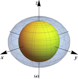
Figure 1: The transverse breathing and the longitudinal polarizations excited by the massive scalar field.

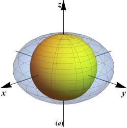
Figure 2: The transverse breathing polarization excited by the massless scalar field.

In summary, the polarizations of gravitational waves in Horndeski theory include the plus and cross polarizations induced by the spin 2 field $\tilde{h}_{\mu\nu}$. The scalar field excites both the transverse breathing and longitudinal polarizations if it is massive. However, if it is massless, the scalar field excites merely the transverse breathing polarization. In terms of the basis introduced for the massless fields in Eardley:1974nw , there are three polarizations: the plus state $\hat{P}_{+}$, the cross state $\hat{P}_{\times}$ and the mix state of $\hat{P}_{b}$ and $\hat{P}_{l}$. In the massless limit, the mix state reduces to the pure state $\hat{P}_{b}$. Note that the vector modes $\hat{P}_{xz}$ and $\hat{P}_{yz}$ are absent in Horndeski theory, this seems to be in conflict with the $E(2)$ classification because the longitudinal mode $\hat{P}_{l}$ is present, so we need to discuss the application of $E(2)$ classification.

3.2 Newman-Penrose variables

Now we calculate the NP variables with the plane wave solution (27) and (28), we get

$$\begin{split}\Psi_{2}=&\frac{1}{12}(R_{txtx}+R_{tyty}-2R_{tztz}\\ &+2R_{xyxy}-R_{xzxz}-R_{yzyz})+\frac{1}{2}iR_{tzxy}\\ =&0,\end{split}$$ (35)

and the nonvanishing ones are

$$\Psi_{4}=-\Omega^{2}(\tilde{h}_{xx}-i\tilde{h}_{xy}),$$ (36)

$$\Phi_{22}=\frac{(q_{t}+\sqrt{q_{t}^{2}-m^{2}})^{2}}{4}\sigma\varphi,$$ (37)

$$\Phi_{00}=\frac{(q_{t}-\sqrt{q_{t}^{2}-m^{2}})^{2}}{(q_{t}+\sqrt{q_{t}^{2}-m^{2}})^{2}}\Phi_{22},$$ (38)

$$\Phi_{11}=\Lambda=\frac{m^{2}}{2(q_{t}+\sqrt{q_{t}^{2}-m^{2}})^{2}}\Phi_{22}.$$ (39)

Note that $\Psi_{2}=-R_{tztz}/6$ for null gravitational waves only, in general case we should use Eq. (35). The naive application of the ELLWW framework to the massive case gives the conclusion that Horndeski gravity has the plus, cross and transverse breathing polarizations, because $\Psi_{2}=\Psi_{3}=0$. Moreover, $\Phi_{00}$ is absent and both $\Phi_{11}$ and $\Lambda$ are proportional to $\Psi_{2}$ in the ELLWW framework, which is in contradiction with Eqs. (38) and Eqs. (39). These indicate the failure of this framework for the massive Horndeski theory. In particular, the absence of $\Psi_{2}$ means that there would be no longitudinal polarization if the ELLWW framework were correct. However, the previous discussion in Section 3.1 clearly shows the existence of the longitudinal polarization. Therefore, the ELLWW framework cannot be applied to a theory which predicts the existence of massive gravitational waves. The massive scalar field excites both the breathing and longitudinal polarizations.

In fact, $R_{tjtk}$ can be rewritten in terms of NP variables as a matrix displayed below,

$$R_{tjtk}=\left(\begin{array}[]{ccc}\Upsilon-\frac{1}{2}\Re\Psi_{4}&\frac{1}{2}\Im\Psi_{4}&0\\ \frac{1}{2}\Im\Psi_{4}&\Upsilon+\frac{1}{2}\Re\Psi_{4}&0\\ 0&0&-2(\Lambda+\Phi_{11})\end{array}\right),$$ (40)

with $\Upsilon=-2\Lambda-\frac{\Phi_{00}+\Phi_{22}}{2}$. It is rather different from Eq. (10). From the above expression, it is clear that some linear combinations of $\Phi_{00}$, $\Phi_{11}$, $\Phi_{22}$ and $\Lambda$ correspond to the transverse breathing and the longitudinal polarizations. In particular, $\Upsilon=-2\Lambda-(\Phi_{00}+\Phi_{22})/2$ represents the transverse breathing polarization, while $-2(\Lambda+\Phi_{11})$ represents the longitudinal polarization. The plus and cross polarizations are still represented by $\Re\Psi_{4}$ and $\Im\Psi_{4}$, respectively. In the massless limit, $\Phi_{00}=\Phi_{11}=\Lambda=0$ according to Eqs. (38) and (39), so Eq. (40) takes the same form as Eq. (10) since the ELLWW framework applies in this case. Note that when the scalar field is massive, Eq. (40) actually takes the same form as Eq. (29) by setting $q_{z}=0$ and $q_{t}=m$ in Eqs. (36), (37), (38) and (39).

These discussion tells us that the detection of polarizations probes the nature of gravity. If only the plus and cross modes are detected, then gravitation is mediated by massless spin 2 field and GR is confirmed. The detection of the breathing mode in addition to the plus and cross modes means that gravitation is mediated by massless spin 2 and spin 0 fields. If the breathing, plus, cross and longitudinal modes are detected, then gravitation is mediated by massless spin 2 and massive spin 0 fields. For the discussion on the detection of polarizations, please see Refs. Isi:2017fbj ; DiPalma:2017qlq .

4 Experimental Tests

4.1 Interferometers

In this subsection, the response functions of the interferometers will be computed for the transverse breathing and longitudinal polarizations following the ideas in Refs Rakhmanov:2004eh ; Corda:2007hi . The detection of GW170104 placed an upper bound on the mass $m_{g}$ of the graviton Abbott:2017vtc ,

$$m_{g}<m_{b}=7.7\times 10^{-23}\,\mathrm{eV}/c^{2}.$$ (41)

In obtaining this bound,the assumed dispersion relation $E^{2}=p^{2}c^{2}+m_{g}^{2}$, leads to dephasing $\delta\Psi(m_{g})$ of the waves relative to the phase evolution in GR, which is given by the template of the waveform predicted by GR. The constraint on $\delta\Psi(m_{g})$ from the observations was used to derive the bound on $m_{g}$. Since there are only the plus and cross polarizations in GR, this bound might not be simply applied to the scalar mode. Whether Eq. (41) can be applied to the scalar graviton is beyond the scope of the present work. Here we assume that the upper bound $m_{b}$ is applicable to the scalar field and study how the upper bound affects the detector responses to the scalar mode. This bound potentially places severe constraint on the effect of the longitudinal polarization on the geodesic deviation in the massive case in the high frequency band, while the transverse breathing mode can be much stronger as long as the amplitude of scalar field $\varphi$ is large enough. Therefore, although there exits the longitudinal mode in the massive scalar-tensor theory, the detection of its effect is likely very difficult in the high frequency band. However, in $f(R)$ gravity, the displacement in the longitudinal direction is independent of the mass and the displacements in the transverse directions become larger for smaller mass, so this mix mode can place strong constraints on $f(R)$ gravity.

In the interferometer, photons emanate from the beam splitter, are bounced back by the mirror and received by the beam splitter again. The round-trip propagation time when the gravitational wave is present is different from that when the gravitational wave is absent. To simplify the calculation of the response functions, the beam splitter is placed at the origin of the coordinate system. Then the change in the round-trip propagation time comes from two effects: the change in the relative distance between the beam splitter and the mirror due to the geodesic deviation, and the distributed gravitational redshift suffered by the photon in the field of the gravitational wave Rakhmanov:2004eh .

First, consider the response function for the longitudinal polarization. To this end, project the light in the $z$ direction and place the mirror at $z=L$. The response function is thus given by,

$$\begin{split}Y_{l}(f)=&\frac{m^{2}}{16\pi^{3}f^{3}}\Big{\{}4\pi fe^{i2\pi fL(v+1)}\\ &-\frac{e^{4i\pi fL}}{\left(v-1\right)^{3}L}\Big{[}e^{i2\pi fL\left(v-1\right)}[2\pi fL\left(v-1\right)\\ &+i2]+2\pi fL\left(v-1\right)-i2\Big{]}\\ &+\frac{1}{\left(v+1\right){}^{3}L}\Big{[}2\pi fL\left(v+1\right)+e^{i2\pi fL\left(v+1\right)}\\ &\left[2\pi fL\left(v+1\right)+2i\right]-i2\Big{]}\Big{\}},\end{split}$$ (42)

where $f=q_{t}/(2\pi)$ is the frequency of gravitational waves and the propagation speed $v$ varies with the frequency. To obtain the response function for the transverse mode, project the light in the $x$ direction and place the mirror at $x=L$. The response function is,

$$Y_{b}(f)=e^{i2\pi fL}+\frac{e^{i2\pi fL}[2\pi fL-\sin(2\pi fL)]}{2\pi fL},$$ (43)

which is independent of the mass $m$ of the scalar field.

Figure 3 shows the absolute values of the longitudinal and transverse response functions for aLIGO ($L=4$ km) to a scalar gravitational wave with the mass $m=m_{b}$. Comparing the response functions shows that the transverse response is much larger than that of the longitudinal mode in high frequencies, so the detection of the longitudinal mode becomes very difficult in the high frequency band.

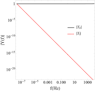
Figure 3: The absolute values of the longitudinal and transverse response functions $|Y_{l}(f)|$ and $|Y_{b}(f)|$ as functions of $f$ for aLIGO ($L=4$ km) to a scalar gravitational wave with the mass $m=m_{b}$ (dashed red curve). The solid curve denotes $|Y_{b}(f)|$ and the dashed curve denotes $|Y_{l}(f)|$.

One can also understand the difficulty to use the interferometers to detect the longitudinal polarizations in the following way. Table 1 lists the magnitudes of $|\ddot{x}^{j}/x^{j}_{0}|$ normalized with $\sigma\varphi$ for the longitudinal and the transverse modes assuming the graviton mass is also $m_{b}$ at three different frequencies: 100 Hz, $10^{-3}$ Hz, and $10^{-7}$ Hz. The first frequency lies in the frequency band of the ground-based detector like aLIGO and VIRGO, the second frequency lies in the frequency band of space-borne observatory like LISA, and the last frequency lies in the sensitive band of pulsar timing arrays Moore:2014lga .

Table 1: The dependence of the magnitudes of $|\ddot{x}^{j}/x^{j}_{0}|$ for the longitudinal and transverse modes on the frequencies of gravitational waves in units of Hz${}^{2}\sigma\varphi$ assuming the scalar mass is $m_{b}$.

	100 Hz	$10^{-3}$ Hz	$10^{-7}$ Hz
Longitudinal	2.81$\times 10^{-15}$	2.81$\times 10^{-15}$	2.81$\times 10^{-15}$
Transverse	$1.97\times 10^{5}$	1.97$\times 10^{-5}$	1.97$\times 10^{-13}$

Table 1 shows that the effect of the longitudinal mode on the geodesic deviation is smaller than that of the transverse mode by 19 to 9 orders of magnitude at higher frequencies. But at the lower frequencies, i.e., at $10^{-7}$ Hz, the two modes have similar amplitudes. Therefore, aLIGO/VIRGO and LISA might find it difficult to detect the longitudinal mode, but pulsar time arrays should be able to detect the mix polarization state with both the longitudinal and transverse modes. The results are consistent with those for the massive graviton in a specific bimetric theory dePaula:2004bc .

4.2 Pulsar Timing Arrays

A pulsar is a rotating neutron star or a white dwarf with a very strong magnetic field. It emits a beam of the electromagnetic radiation. When the beam points towards the Earth, the radiation can be observed, which explains the pulsed appearance of the radiation. Millisecond pulsars can be used as stable clocks Verbiest:2009kb . When there is no gravitational wave, one can observe the pulses at a steady rate. The presence of the gravitational wave will alter this rate, because it will affect the propagation time of the radiation. This will lead to a change in the time-of-arrival (TOA), called time residual $R(t)$. Time residuals caused by the gravitational wave will be correlated between pulsars, and the cross-correlation function is $C(\theta)=\langle R_{a}(t)R_{b}(t)\rangle$, where $\theta$ is the angular separation of pulsars $a$ and $b$, and the brackets $\langle\,\rangle$ imply the ensemble average over the stochastic background. This enables the detection of gravitational waves and the probe of the polarizations.

The effects of the gravitational wave in GR on the time residuals were first considered in Refs 1975GReGr…6..439E ; 1978SvA….22…36S ; Detweiler:1979wn . Hellings and Downs Hellings:1983fr proposed a method to detect the effects by using the cross-correlation of the time derivative of the time residuals between pulsars, while Jenet et. al. Jenet:2005pv directly worked with the time residuals instead of the time derivative. The later work was generalized to massless gravitational waves in alternative metric theories of gravity in Ref. 2008ApJ…685.1304L , and further to massive gravitational waves in Refs Lee:2010cg ; Lee:2014awa . More works have been done, for example, Refs Chamberlin:2011ev ; Yunes:2013dva ; Gair:2014rwa ; Gair:2015hra and references therein.

In their treatments, it is assumed that all the polarization modes have the same mass, either zero or not. If all polarizations propagate in the $+z$ direction at the speed of light, there will be three linearly independent Killing vector fields, $\chi_{1}^{\mu}=\delta^{\mu}_{1},\,\chi_{2}^{\mu}=\delta_{2}^{\mu}$, and $\chi_{3}^{\mu}=\delta^{\mu}_{0}+\delta^{\mu}_{3}$. Using the conservation of $p_{\mu}\chi^{\mu}_{j}$ ($j=1,2,3$) for photon’s 4-velocity $p^{\mu}$ satisfying $p^{\nu}\nabla_{\nu}p^{\mu}=0$, one obtains the change in the locally observed frequency of the radiation and integrates to obtain the time residual $R(t)$ 1975GReGr…6..439E ; Burke:1975zz ; Tinto:2010hz . One could also directly integrate the time component of the photon geodesic equation to obtain the change in the frequency Anholm:2008wy ; Lee:2010cg . The later method can be applied to massive case. In the present work, a different method will be used by simply calculating the 4-velocities of the photon and observers on the Earth and the pulsar. Since different polarizations propagate at different speeds, there are not enough linearly independent Killing vector fields. The first method cannot be used any way.

In order to calculate the time residual $R(t)$ caused by the gravitational wave solution (27) and (28), one sets up a coordinate system shown in Figure 4, so that when there is no gravitational wave, the Earth is at the origin, and the distant pulsar is assumed to be stationary in the coordinate system and one can always orient the coordinate system such that the pulsar is located at $\vec{x}_{p}=(L\cos\beta,0,L\sin\beta)$. $\hat{q}_{z}$ is the unit vector pointing to the direction of the gravitational wave, $\hat{n}$ is the unit vector connecting the Earth to the pulsar, and $\hat{l}=\hat{q}_{z}\wedge(\hat{n}\wedge\hat{q}_{z})/\cos\beta=[\hat{n}-\hat{q}_{z}(\hat{n}\cdot\hat{q}_{z})]/\cos\beta$ is the unit vector parallel to the $y$ axis.

Figure 4: The gravitational wave is propagating in the direction of $\hat{q}_{z}$, and the photon is traveling in $-\hat{n}$ direction at the leading order. $\hat{l}$ is perpendicular to $\hat{q}_{z}$ and in the same plane determined by $\hat{q}_{z}$ and $\hat{n}$. The angle between $\hat{n}$ and $\hat{l}$ is $\beta$.

In the leading order, i.e., in the absence of gravitational waves, the 4-velocity of the photon is $\underline{u}^{\mu}=\gamma_{0}(1,-\cos\beta,0,-\sin\beta)$ with $\gamma_{0}=\mathrm{d}t/\mathrm{d}\lambda$ a constant and $\lambda$ an arbitrary affine parameter. The perturbed photon 4-velocity is $u^{\mu}=\underline{u}^{\mu}+v^{\mu}$, and since $g_{\mu\nu}u^{\mu}u^{\nu}=0$, one obtains

$$v^{0}=\frac{\gamma_{0}}{2}\tilde{h}_{11}\cos^{2}\beta-v_{1}\cos\beta-v_{3}\sin\beta.$$ (44)

Note that one chooses the gauge such that $e_{11}=-e_{22}$, $e_{12}=e_{21}$ are the only nonvanishing amplitudes for $\tilde{h}_{\mu\nu}$, which can always be made. The photon geodesic equation is

$$\begin{split}0=&\frac{\mathrm{d}u^{\mu}}{\mathrm{d}\lambda}+\Gamma^{\mu}{}_{\rho\sigma}u^{\rho}u^{\sigma}\\ \approx&\gamma_{0}\frac{\mathrm{d}u^{\mu}}{\mathrm{d}t}+\Gamma^{\mu}{}_{\rho\sigma}\underline{u}^{\rho}\underline{u}^{\sigma}.\end{split}$$ (45)

The calculation shows that

$$v^{0} = \gamma_{0}\Big{\{}\sigma\varphi_{0}\cos[(q_{t}+q_{z}\sin\beta)t-q_{z}(L+t_{e})\sin\beta]$$ (46)

$$-\frac{e_{11}}{2}(1-\sin\beta)\cos[\Omega(1+\sin\beta)t$$

$$-\Omega(L+t_{e})\sin\beta]\Big{\}},$$

$$v_{1} = \gamma_{0}\{-\sigma\varphi_{0}\cos\beta\cos[(q_{t}+q_{z}\sin\beta)t-q_{z}(L+t_{e})\sin\beta]$$ (47)

$$+e_{11}\cos\beta\cos[\Omega(1+\sin\beta)t-\Omega(L+t_{e})\sin\beta]\},$$

$$v_{2} = \gamma_{0}e_{12}\cos\beta\cos\Omega[(1+\sin\beta)t-(L+t_{e})\sin\beta],$$ (48)

$$v_{3} = \gamma_{0}\Big{\{}-\sigma\varphi_{0}\sin\beta\cos[(q_{t}+q_{z}\sin\beta)t-q_{z}(L+t_{e})\sin\beta]$$ (49)

$$-\frac{e_{11}}{2}(1-\sin\beta)\cos[\Omega(1+\sin\beta)t$$

$$-\Omega(L+t_{e})\sin\beta]\Big{\}},$$

where $t_{e}$ is the time when the photon is emitted from the pulsar. Eq. (46) is consistent with Eq. (44).

The 4-velocities of the Earth and the pulsar also change due to the gravitational wave. Take the 4-velocity of the Earth for instance. Suppose when the gravitational wave is present, its 4-velocity is given by $u_{e}^{\mu}=u_{e}^{0}(1,\vec{v}_{e})$. The normalization of $u^{\mu}_{e}$ implies that

$$u^{0}_{e}=1+\frac{1}{2}h_{00}+O(v_{e}^{2}).$$ (50)

The geodesic equation for the Earth is,

$$\begin{split}0=&\frac{\mathrm{d}^{2}x^{\mu}}{\mathrm{d}\tau^{2}}+\Gamma^{\mu}{}_{\rho\nu}\frac{\mathrm{d}x^{\rho}}{\mathrm{d}\tau}\frac{\mathrm{d}x^{\nu}}{\mathrm{d}\tau}\\ \approx&(u^{0}_{e})^{2}\left(\frac{\mathrm{d}^{2}x^{\mu}}{\mathrm{d}t^{2}}+\Gamma^{\mu}{}_{00}\right)+u^{0}_{e}\frac{\mathrm{d}u^{0}_{e}}{\mathrm{d}t}\frac{\mathrm{d}x^{\mu}}{\mathrm{d}t},\end{split}$$ (51)

where $\tau$ is the proper time and $x^{\mu}$ are the coordinates of the Earth. One sets $x=y=0$, which is consistent with Eq. (51). Then, one obtains the following solution

$$v^{3}_{e}\approx-\frac{q_{z}}{2q_{t}}\sigma\varphi_{0}\cos q_{t}t.$$ (52)

In addition, with Eq. (50),

$$u^{0}_{e}=1+\frac{1}{2}\sigma\varphi_{0}\cos q_{t}t.$$ (53)

So the 4-velocity of the Earth is approximately

$$u^{\mu}_{e}=\left(1+\frac{1}{2}\sigma\varphi_{0}\cos q_{t}t,0,0,-\frac{q_{z}}{2q_{t}}\sigma\varphi_{0}\cos q_{t}t\right).$$ (54)

Similarly, one can obtain the 4-velocity of the pulsar, which is

$$\begin{split}u^{\mu}_{p}=&\left(1+\frac{1}{2}\sigma\varphi_{0}\cos(q_{t}t-q_{z}L\sin\beta),0,\right.\\ &\left.0,-\frac{q_{z}}{2q_{t}}\sigma\varphi_{0}\cos(q_{t}t-q_{z}L\sin\beta)\right),\end{split}$$ (55)

up to linear order. The form of $u^{\mu}_{p}$ can be understood, realizing that $\chi_{1}^{\mu}$ and $\chi_{2}^{\mu}$ are still the Killing vector fields.

Therefore, the frequency of the photon measured by an observer comoving with the pulsar is

$$\begin{split}f_{e}=&-u_{\mu}u^{\mu}_{p}\\ =&\gamma_{0}\Big{[}1+\frac{q_{t}-q_{z}\sin\beta}{2q_{t}}\sigma\varphi_{0}\cos(q_{t}t_{e}-q_{z}L\sin\beta)\\ &-\frac{e_{11}}{2}(1-\sin\beta)\cos\Omega(t_{e}-L\sin\beta)\Big{]},\end{split}$$ (56)

and the frequency measured by another observer on the Earth is

$$\begin{split}f_{r}=&-u_{\mu}u^{\mu}_{e}\\ =&\gamma_{0}\Big{[}1+\frac{q_{t}-q_{z}\sin\beta}{2q_{t}}\sigma\varphi_{0}\cos q_{t}(t_{e}+L)\\ &-\frac{e_{11}}{2}(1-\sin\beta)\cos\Omega(t_{e}+L)\Big{]}.\end{split}$$ (57)

The frequency shift is thus given by

$$\begin{split}\frac{f_{e}-f_{r}}{f_{r}}=&\frac{q_{t}-q_{z}\hat{q}_{z}\cdot\hat{n}}{2q_{t}}\sigma\left[\varphi(t-L,L\hat{n})-\varphi(t,0)\right]\\ &-\frac{\hat{n}^{j}\hat{n}^{k}}{2(1+\hat{q}_{z}\cdot\hat{n})}\left[\tilde{h}_{jk}(t-L,L\hat{n})-\tilde{h}_{jk}(t,0)\right],\end{split}$$ (58)

where $t=t_{e}+L$ is the time when the photon arrives at the Earth at the leading order. This expression (58) can be easily generalized to a coordinate system with an arbitrary orientation and at rest relative to the original frame. It can be checked that in the massless limit, the change in the ratio of frequencies agrees with Eq. (2) in Ref. 2008ApJ…685.1304L . The contribution of the massive scalar field also agrees with Eq. (2) in Ref. Lee:2014awa which was derived provided all polarizations have the same mass.

Eq. (58) gives the frequency shift caused by a monochromatic gravitational wave. Now, consider the contribution of a stochastic gravitational wave background which consists of monochromatic gravitational waves,

$$\tilde{h}_{jk}(t,\vec{x})=$$

$$\sum_{P=+,\times}\int_{-\infty}^{\infty}\frac{\mathrm{d}\Omega}{2\pi}\int\mathrm{d}^{2}\hat{k}\Big{\{}\tilde{h}^{P}(\Omega,\hat{k})\epsilon^{P}_{jk}\exp[i\Omega(t-\hat{k}\cdot\vec{x})]\Big{\}},$$ (59)

$$\varphi(t,\vec{x})=$$

$$\int_{-\infty}^{\infty}\frac{\mathrm{d}q_{t}}{2\pi}\int\mathrm{d}^{2}\hat{q}_{z}\Big{\{}\varphi_{0}(q_{t},\hat{q}_{z})\exp[i(q_{t}t-q_{z}\hat{q}_{z}\cdot\vec{x})]\Big{\}},$$ (60)

where $\tilde{h}^{P}(\Omega,\hat{k})$ is the amplitude of the gravitational wave propagating in the direction $\hat{k}$ at the angular frequency $\Omega$ with the polarization $P=+$ or $\times$, $\epsilon^{P}_{jk}$ is the polarization tensor for the polarization $P$, and $\varphi_{0}(q_{t},\hat{q}_{z})$ is the amplitude for the scalar gravitational wave propagating in the direction $\hat{q}_{z}$ at the angular frequency $q_{t}$. Let $\hat{i},\,\hat{j},\,\hat{k}$ form a right-handed triad frame so that $\hat{i}\times\hat{j}=\hat{k}$, then $\epsilon^{P}_{jk}$ is given by

$$\epsilon^{+}_{jk}=\hat{i}_{j}\hat{i}_{k}-\hat{j}_{j}\hat{j}_{k},\quad\epsilon^{\times}_{jk}=\hat{i}_{j}\hat{j}_{k}+\hat{j}_{j}\hat{i}_{k}.$$ (61)

Assuming the gravitational wave background is isotropic, stationary and independently polarized, one defines the characteristic strains $\tilde{h}^{P}_{c}$ and $\varphi_{c}$ in the following way,

$$\langle\tilde{h}^{P*}(\Omega,\hat{k})\tilde{h}^{P^{\prime}}(\Omega^{\prime},\hat{k}^{\prime})\rangle=$$

$$\delta(\Omega-\Omega^{\prime})\delta(\hat{k}-\hat{k}^{\prime})\delta^{PP^{\prime}}\frac{\pi|\tilde{h}_{c}^{P}|^{2}(\Omega)}{4\Omega},$$ (62)

$$\langle\varphi_{0}^{*}(q_{t},\hat{q}_{z})\varphi_{0}(q^{\prime}_{t},\hat{q}^{\prime}_{z})\rangle=\delta(q_{t}-q^{\prime}_{t})\delta(\hat{q}_{z}-\hat{q}^{\prime}_{z})\frac{|\varphi_{c}|^{2}(q_{t})}{q_{t}},$$ (63)

where the star $*$ indicates the complex conjugation.

Since the gravitational wave with the plus or cross polarization behaves exactly the same way as in GR which can be found in Ref. 2008ApJ…685.1304L , the focus will be on the contribution of the scalar field in the following discussion. The total time residual in TOA caused by the stochastic gravitational wave background is

$$R(T)=\int_{-\infty}^{\infty}\frac{\mathrm{d}q_{t}}{2\pi}\int\mathrm{d}^{2}\hat{q}_{z}\int_{0}^{T}\mathrm{d}t\frac{f_{e}-f_{r}}{f_{r}},$$ (64)

where the argument $T$ is the total observation time. Substituting Eq. (58) (ignoring the second line) in, one obtains

$$\begin{split}R(T)=&\int_{-\infty}^{\infty}\frac{\mathrm{d}q_{t}}{2\pi}\int\mathrm{d}^{2}\hat{q}_{z}\frac{q_{t}-q_{z}\hat{q}_{z}\cdot\hat{n}}{i2q_{t}^{2}}\varphi_{0}(q_{t},\hat{q}_{z})(e^{iq_{t}T}-1)\times\\ &[1-e^{-i(q_{t}+q_{z}\hat{q}_{z}\cdot n)L}].\end{split}$$ (65)

Therefore, one can now consider the correlation between two pulsars $a$ and $b$ which are located at positions $\vec{x}_{a}=L_{1}\hat{n}_{1}$ and $\vec{x}_{b}=L_{2}\hat{n}_{2}$, respectively. The angular separation is $\theta=\arccos(\hat{n}_{1}\cdot\hat{n}_{2})$. The cross-correlation function is thus given by

$$\begin{split}C(\theta)=&\langle R_{a}(T)R_{b}(T)\rangle\\ =&\int_{m}^{\infty}\mathrm{d}q_{t}\int\mathrm{d}^{2}\hat{q}_{z}\frac{(q_{t}-q_{z}\hat{q}_{z}\cdot\hat{n}_{1})(q_{t}-q_{z}\hat{q}_{z}\cdot\hat{n}_{2})}{4\pi^{2}q_{t}^{5}}\times\\ &|\varphi_{c}|^{2}(q_{t})\mathcal{P},\end{split}$$ (66)

where

$$\mathcal{P}=1-\cos\Delta_{1}-\cos\Delta_{2}+\cos(\Delta_{1}-\Delta_{2}),$$ (67)

and $\Delta_{j}=(q_{t}+q_{z}\hat{q}_{z}\cdot\hat{n}_{j})L_{j}$ with $j=1,2$. In obtaining this result, one uses Eq. (63), and takes the real part. In addition, $T$ drops out, since the ensemble average also implies the average over the time 2008ApJ…685.1304L .

Since the gravitational wave background is assumed to be isotropic, one can calculate $C(\theta)$ by setting

$$\hat{n}_{1}=(0,0,1),$$ (68)

$$\hat{n}_{2}=(\sin\theta,0,\cos\theta).$$ (69)

Also, let $\hat{q}_{z}=(\sin\theta_{g}\cos\phi_{g},\sin\theta_{g}\sin\phi_{g},\cos\theta_{g})$, so

$$\Delta_{1}=(q_{t}+q_{z}\cos\theta_{g})L_{1},$$ (70)

$$\Delta_{2}=[q_{t}+q_{z}(\sin\theta_{g}\cos\phi_{g}\sin\theta+\cos\theta_{g}\cos\theta)]L_{2},$$ (71)

and

$$\begin{split}C(\theta)=&\int_{m}^{\infty}\mathrm{d}q_{t}\int\mathrm{d}\theta_{g}\mathrm{d}\phi_{g}\sin\theta_{g}\frac{|\varphi_{c}|^{2}(q_{t})}{4\pi^{2}q_{t}^{5}}(q_{t}-q_{z}\cos\theta_{g})\\ &[q_{t}-q_{z}(\sin\theta_{g}\cos\phi_{g}\sin\theta+\cos\theta_{g}\cos\theta)]\mathcal{P}.\end{split}$$ (72)

In the observation, pulsars are far away enough, so that $q_{t}L_{j}\gg 1$. This implies that one can approximate $\mathcal{P}\approx 1$ when $\theta\neq 0$, as the phases in cosines in the definition (67) of $\mathcal{P}$ oscillate fast enough. The integration can be partially done, yielding

$$C(\theta)\approx\int_{m}^{\infty}\mathrm{d}q_{t}\frac{|\varphi_{c}|^{2}(q_{t})}{\pi q_{t}^{3}}\left(1+\frac{q_{z}^{2}}{3q_{t}^{2}}\cos\theta\right).$$ (73)

But for $\theta=0$, one cannot simply set cosines in $\mathcal{P}$ to 1. In this case, one actually considers the auto-correlation function, so $\hat{n}_{1}=\hat{n}_{2}$ and $L_{1}=L_{2}=L$. The auto-correlation function is thus given by

$$\begin{split}C(0)=&2\int_{m}^{\infty}\mathrm{d}q_{t}\frac{|\varphi_{c}|^{2}(q_{t})}{\pi q_{t}^{3}}\left[1+\frac{q_{z}^{2}}{3q_{t}^{2}}+\frac{2}{q_{t}^{2}L^{2}}\cos q_{t}L\cos q_{z}L\right.\\ &\left.+\left(\frac{2}{q_{t}L}-\frac{1}{q_{z}L}+\frac{2}{q_{t}^{2}q_{z}L^{3}}-\frac{q_{z}}{q_{t}^{2}L}\right)\cos q_{t}L\sin q_{z}L\right.\\ &\left.-\frac{2}{q_{t}q_{z}L^{2}}\sin q_{t}L\sin q_{z}L\right].\end{split}$$ (74)

Note that the observation time $T$ sets a natural cutoff for the frequency, i.e., $q_{t}\geq 2\pi/T$. So the lower integration limits in Eqs. (73) and (74) should be replaced by $\text{Min}\{m,2\pi/T\}$.

Usually, one assumes that $\varphi_{c}(q_{t})$ takes a form of $\varphi_{c}(q_{t})\propto(q_{t}/q_{t}^{c})^{\alpha}$ with $q_{t}^{c}$ some characteristic angular frequency. $\alpha$ is called the power-law index, and usually, $\alpha=0,\,-2/3$ or $-1$ 2008ApJ…685.1304L ; Romano:2016dpx . One can numerically integrate Eqs. (73) and (74) to obtain the so-called normalized correlation function $\zeta(\theta)=C(\theta)/C(0)$. In the integration, suppose the observation time $T=5$ years and the mass of the scalar field is $m_{b}=7.7\times 10^{-23}$ eV$/c^{2}$ Abbott:2017vtc . The distance $L$ takes a large enough value so that $q_{t}L\gg 1$ is satisfied. This gives rise to the right panel in Figure 5, where the power-law index $\alpha$ takes different values. Together shown are the normalized correlation functions for the plus and cross polarizations (labeled by “GR"), and for the transverse breathing polarization (labeled by “Breathing") in the left panel. The normalized correlation function for the transverse breathing polarization can be obtained simply by setting the mass $m=0$.

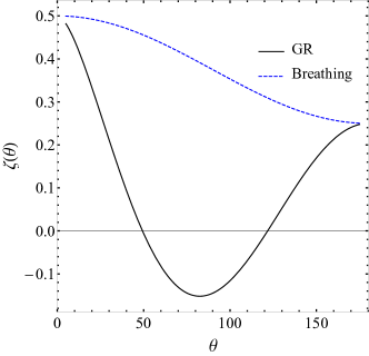
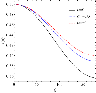
Figure 5: The normalized cross-correlation functions $\zeta(\theta)=C(\theta)/C(0)$. The upper panel shows the cross-correlations when the scalar field is massless, i.e., when there is no longitudinal polarization. The solid curve is for familiar GR polarizations (i.e., the plus or cross ones), and the dashed curve for the transverse breathing polarization. The lower panel shows the cross-correlations induced together by the transverse breathing and longitudinal polarizations when the mass of the scalar field is taken to be $m_{b}=7.7\times 10^{-23}\,\mathrm{eV}/c^{2}$. The calculation was done assuming $T=5$ yrs.

It is clear that $\zeta(\theta)$ behaves very differently for $\tilde{h}_{\mu\nu}$ and $\varphi$, so it is possible to determine whether there are polarizations induced by the scalar field using pulsar timing arrays. Note that since $L$ is large enough, $\zeta(\theta)$ barely changes with $L$.

One could also vary the mass of the scalar field. The result is shown in Figure 6. This figure displays $\zeta(\theta)$ for six different multiples of $m_{b}$, including $m=0$ labeled by “Breathing". The power-law index $\alpha$ is chosen to be 0. It shows that at large angles, $\zeta(\theta)$ is very sensitive to smaller masses with $m_{b}/5\lesssim m\lesssim m_{b}$, but for $m\gtrsim m_{b}$ or $m\lesssim m_{b}/5$, $\zeta(\theta)$ almost remains the same. Therefore, the measurement of the correlation can be used to constrain the mass of the scalar field.

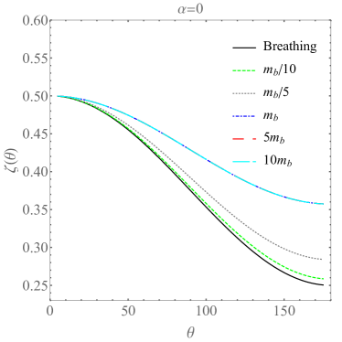
Figure 6: $\zeta(\theta)$ as a function of scalar mass $m$ at $\alpha=0$. The calculations were also done for a 5-year observation.

In Ref. Lee:2014awa , Lee also analyzed the time residual of TOA caused by massive gravitational waves and calculated the cross-correlation functions. His results (the right two panels in his Figure 1) differ from those on the right panel in Figure 5, because in his treatment, the longitudinal and the transverse polarizations were assumed to be independent. In Horndeski theory, however, it is not allowed to calculate the cross-correlation function separately for the longitudinal and the transverse polarizations, as they are both excited by the same field $\varphi$ and the polarization state is a single mode.

5 Conclusion

This work analyzes the gravitational wave polarizations in the most general scalar-tensor theory of gravity, Horndeski theory. It reveals that there are three independent polarization modes: the mixture state of the transverse breathing $\hat{P}_{b}=R_{txtx}+R_{tyty}$ and longitudinal $\hat{P}_{l}=R_{tztz}$ polarizations for the massive scalar field, and the usual plus $\hat{P}_{+}=-R_{txtx}+R_{tyty}$ and cross $\hat{P}_{\times}=R_{txty}$ polarizations for the massless gravitons. These results are consistent with the three propagating degrees of freedom in Horndeski theory. Since the propagation speed of the massive gravitational wave depends on the frequency and is smaller than the speed of light, the massive mode will arrive at the detector later than the massless gravitons. In addition to the difference of the propagation speed, the presence of both the longitudinal and breathing states without the vector-$x$ and vector-$y$ states are also the distinct signature of massive scalar degree of freedom for graviton.

Using the NP variables, we find that $\Psi_{2}=0$. For null gravitational waves, this means that the longitudinal mode does not exist. However, our results show that the longitudinal mode exists in the massive case even though $\Psi_{2}=0$. We also find that the NP variable $\Phi_{00}\neq 0$, and $\Phi_{00}$, $\Phi_{11}$ and $\Lambda$ are all proportional to $\Phi_{22}$. These results are in conflict with those for massless gravitational waves in Eardley:1974nw , so the results further support the conclusion that the classification of the six polarizations for null gravitational waves derived from the little group $E(2)$ of the Lorentz group is not applicable to the massive case. Although the longitudinal mode exists for the massive scalar field, it is difficult to be detected in the high frequency band because of the suppression by the extremely small graviton mass upper bound. Compared with aLIGO/VIRGO and LISA, pulsar timing arrays might be the primary tool to detect both the transverse breathing and longitudinal modes due to the massive scalar field. In the massless case, the longitudinal mode disappears and the mix state reduces to the pure transverse breathing mode. Brans-Dicke theory and $f(R)$ gravity are subclasses of Horndeski theory, so the general results obtained can be applied to those theories. Despite the fact that in $f(R)$ gravity, the longitudinal mode does not depend on the mass of graviton, its magnitude is much smaller than the transverse one in the high frequency band, which makes its detection unlikely by the network of aLIGO/VIGO and LISA, too. It is interesting that the transverse mode becomes stronger for smaller graviton mass in the $f(R)$ gravity, so the detection of the mixture state can place strong constraint on $f(R)$ gravity.

For null gravitational waves, the presence of the longitudinal mode means that all six polarizations can be detected in some coordinate systems. For Horndeski theory, we find that the vector modes are absent even though the longitudinal mode is present. Since the massive scalar field excites both the breathing and longitudinal polarizations, while the massless scalar field excites the breathing mode only, the detection of polarizations can be used to understand the nature of gravity. If only the plus and cross modes are detected, then gravitation is mediated by massless spin 2 field and GR is confirmed. The detection of the breathing mode in addition to the plus and cross modes means that gravitation is mediated by massless spin 2 and spin 0 fields. If the breathing, plus, cross and longitudinal modes are detected, then gravitation is mediated by massless spin 2 and massive spin 0 fields.

- (1) B.P. Abbott, et al., Observation of Gravitational Waves from a Binary Black Hole Merger. Phys. Rev. Lett. 116(6), 061102 (2016)
- (2) B.P. Abbott, et al., GW151226: Observation of Gravitational Waves from a 22-Solar-Mass Binary Black Hole Coalescence. Phys. Rev. Lett. 116(24), 241103 (2016)
- (3) B.P. Abbott, et al., GW170104: Observation of a 50-Solar-Mass Binary Black Hole Coalescence at Redshift 0.2. Phys. Rev. Lett. 118(22), 221101 (2017)
- (4) B.P. Abbott, et al., GW170814: A Three-Detector Observation of Gravitational Waves from a Binary Black Hole Coalescence. Phys. Rev. Lett. 119(14), 141101 (2017)
- (5) B.P. Abbott, et al., GW170817: Observation of Gravitational Waves from a Binary Neutron Star Inspiral. Phys. Rev. Lett. 119(16), 161101 (2017)
- (6) B.P. Abbott, et al., GW170608: Observation of a 19-solar-mass Binary Black Hole Coalescence. Astrophys. J. 851(2), L35 (2017)
- (7) H. Audley, et al., Laser Interferometer Space Antenna. arXiv:1702.00786
- (8) J. Luo, et al., TianQin: a space-borne gravitational wave detector. Class. Quant. Grav. 33(3), 035010 (2016)
- (9) G. Hobbs, et al., The international pulsar timing array project: using pulsars as a gravitational wave detector. Class. Quant. Grav. 27, 084013 (2010)
- (10) M. Kramer, D.J. Champion, The European Pulsar Timing Array and the Large European Array for Pulsars. Class. Quant. Grav. 30, 224009 (2013)
- (11) B.P. Abbott, et al., First search for nontensorial gravitational waves from known pulsars. Phys. Rev. Lett. 120(3), 031104 (2018)
- (12) A. Goldstein, et al., An Ordinary Short Gamma-Ray Burst with Extraordinary Implications: Fermi-GBM Detection of GRB 170817A. Astrophys. J. Lett. 848(2), L14 (2017)
- (13) V. Savchenko, et al., INTEGRAL Detection of the First Prompt Gamma-Ray Signal Coincident with the Gravitational-wave Event GW170817. Astrophys. J. Lett. 848(2), L15 (2017)
- (14) M. Isi, A.J. Weinstein, C. Mead, M. Pitkin, Detecting Beyond-Einstein Polarizations of Continuous Gravitational Waves. Phys. Rev. D 91(8), 082002 (2015)
- (15) M. Isi, M. Pitkin, A.J. Weinstein, Probing Dynamical Gravity with the Polarization of Continuous Gravitational Waves. Phys. Rev. D 96(4), 042001 (2017)
- (16) E. Newman, R. Penrose, An Approach to gravitational radiation by a method of spin coefficients. J. Math. Phys. 3, 566 (1962)
- (17) D.M. Eardley, D.L. Lee, A.P. Lightman, Gravitational-wave observations as a tool for testing relativistic gravity. Phys. Rev. D 8, 3308 (1973)
- (18) D.M. Eardley, D.L. Lee, A.P. Lightman, R.V. Wagoner, C.M. Will, Gravitational-wave observations as a tool for testing relativistic gravity. Phys. Rev. Lett. 30, 884 (1973)
- (19) C. Brans, R. Dicke, Mach’s principle and a relativistic theory of gravitation. Phys. Rev. 124, 925 (1961)
- (20) G.W. Horndeski, Second-order scalar-tensor field equations in a four-dimensional space. Int. J. Theor. Phys. 10, 363 (1974)
- (21) M. Ostrogradsky, Mémoires sur les équations différentielles, relatives au problème des isopérimètres. Mem. Acad. St. Petersbourg 6(4), 385 (1850)
- (22) R. Utiyama, B.S. DeWitt, Renormalization of a classical gravitational field interacting with quantized matter fields. J. Math. Phys. 3, 608 (1962)
- (23) K. Stelle, Renormalization of Higher Derivative Quantum Gravity. Phys. Rev. D 16, 953 (1977)
- (24) K.S. Stelle, Classical Gravity with Higher Derivatives. Gen. Rel. Grav. 9, 353 (1978)
- (25) H.A. Buchdahl, Non-linear Lagrangians and cosmological theory. Mon. Not. Roy. Astron. Soc. 150, 1 (1970)
- (26) J. O’ Hanlon, Intermediate-range gravity - a generally covariant model. Phys. Rev. Lett. 29, 137 (1972)
- (27) P. Teyssandier, P. Tourrenc, The Cauchy problem for the R+R**2 theories of gravity without torsion. J. Math. Phys. 24, 2793 (1983)
- (28) C. Corda, The production of matter from curvature in a particular linearized high order theory of gravity and the longitudinal response function of interferometers. JCAP 0704, 009 (2007)
- (29) C. Corda, Massive gravitational waves from the R**2 theory of gravity: Production and response of interferometers. Int. J. Mod. Phys. A 23, 1521 (2008)
- (30) S. Capozziello, C. Corda, M.F. De Laurentis, Massive gravitational waves from f(R) theories of gravity: Potential detection with LISA. Phys. Lett. B 669, 255 (2008)
- (31) S. Capozziello, R. Cianci, M. De Laurentis, S. Vignolo, Testing metric-affine f(R)-gravity by relic scalar gravitational waves. Eur. Phys. J. C 70, 341 (2010)
- (32) P. Prasia, V.C. Kuriakose, Detection of massive Gravitational Waves using spherical antenna. Int. J. Mod. Phys. D 23, 1450037 (2014)
- (33) M.E.S. Alves, O.D. Miranda, J.C.N. de Araujo, Probing the f(R) formalism through gravitational wave polarizations. Phys. Lett. B 679, 401 (2009)
- (34) M.E.S. Alves, O.D. Miranda, J.C.N. de Araujo, Extra polarization states of cosmological gravitational waves in alternative theories of gravity. Class. Quant. Grav. 27, 145010 (2010)
- (35) H.R. Kausar, L. Philippoz, P. Jetzer, Gravitational Wave Polarization Modes in Theories. Phys. Rev. D 93(12), 124071 (2016)
- (36) Y.S. Myung, Propagating degrees of freedom in f(R) gravity. Adv. High Energy Phys. 2016, 3901734 (2016)
- (37) D. Liang, Y. Gong, S. Hou, Y. Liu, Polarizations of gravitational waves in gravity. Phys. Rev. D 95(10), 104034 (2017)
- (38) Y. Gong, S. Hou, Gravitational Wave Polarizations in Gravity and Scalar-Tensor Theory. EPJ Web Conf. 168, 01003 (2018)
- (39) Y. Gong, S. Hou, D. Liang, E. Papantonopoulos, Gravitational waves in Einstein-æther and generalized TeVeS theory after GW170817. Phys. Rev. D 97, 084040 (2018)
- (40) Q. Gao, Y. Gong, D. Liang, The polarizations of gravitational waves. Chin. Sci. Bull. 63(9), 801 (2018)
- (41) T. Kobayashi, M. Yamaguchi, J. Yokoyama, Generalized G-inflation: Inflation with the most general second-order field equations. Prog.Theor.Phys. 126, 511 (2011)
- (42) M. Isi, A.J. Weinstein, Probing gravitational wave polarizations with signals from compact binary coalescences. arXiv:1710.03794
- (43) I. Di Palma, M. Drago, Estimation of the gravitational wave polarizations from a nontemplate search. Phys. Rev. D 97(2), 023011 (2018)
- (44) M. Rakhmanov, Response of test masses to gravitational waves in the local Lorentz gauge. Phys. Rev. D 71, 084003 (2005)
- (45) C.J. Moore, R.H. Cole, C.P.L. Berry, Gravitational-wave sensitivity curves. Class. Quant. Grav. 32(1), 015014 (2015)
- (46) W.L.S. de Paula, O.D. Miranda, R.M. Marinho, Polarization states of gravitational waves with a massive graviton. Class. Quant. Grav. 21, 4595 (2004)
- (47) J.P.W. Verbiest, et al., Timing stability of millisecond pulsars and prospects for gravitational-wave detection. Mon. Not. Roy. Astron. Soc. 400, 951 (2009)
- (48) F.B. Estabrook, H.D. Wahlquist, Response of Doppler spacecraft tracking to gravitational radiation. Gen. Rel. Grav. 6, 439 (1975)
- (49) M.V. Sazhin, Opportunities for detecting ultralong gravitational waves. Sov. Astron. 22, 36 (1978)
- (50) S.L. Detweiler, Pulsar timing measurements and the search for gravitational waves. Astrophys. J. 234, 1100 (1979)
- (51) R.W. Hellings, G.S. Downs, Upper limits on the isotropic graviational radiation background from pulsar timing analysis. Astrophys. J. 265, L39 (1983)
- (52) F.A. Jenet, G.B. Hobbs, K.J. Lee, R.N. Manchester, Detecting the stochastic gravitational wave background using pulsar timing. Astrophys. J. 625, L123 (2005)
- (53) K.J. Lee, F.A. Jenet, R.H. Price, Pulsar Timing as a Probe of Non-Einsteinian Polarizations of Gravitational Waves. Astrophys. J. 685, 1304-1319 (2008)
- (54) K. Lee, F.A. Jenet, R.H. Price, N. Wex, M. Kramer, Detecting massive gravitons using pulsar timing arrays. Astrophys. J. 722, 1589 (2010)
- (55) K.J. Lee, Pulsar Timing Arrays and Gravity Tests in the Radiative Regime. Class. Quant. Grav. 30, 224016 (2013)
- (56) S.J. Chamberlin, X. Siemens, Stochastic backgrounds in alternative theories of gravity: overlap reduction functions for pulsar timing arrays. Phys. Rev. D 85, 082001 (2012)
- (57) N. Yunes, X. Siemens, Gravitational-Wave Tests of General Relativity with Ground-Based Detectors and Pulsar Timing-Arrays. Living Rev. Rel. 16, 9 (2013)
- (58) J. Gair, J.D. Romano, S. Taylor, C.M.F. Mingarelli, Mapping gravitational-wave backgrounds using methods from CMB analysis: Application to pulsar timing arrays. Phys. Rev. D 90(8), 082001 (2014)
- (59) J.R. Gair, J.D. Romano, S.R. Taylor, Mapping gravitational-wave backgrounds of arbitrary polarisation using pulsar timing arrays. Phys. Rev. D 92(10), 102003 (2015)
- (60) W.L. Burke, Large-Scale Random Gravitational Waves. Astrophys. J. 196, 329 (1975)
- (61) M. Tinto, M.E. da Silva Alves, LISA Sensitivities to Gravitational Waves from Relativistic Metric Theories of Gravity. Phys. Rev. D 82, 122003 (2010)
- (62) M. Anholm, S. Ballmer, J.D.E. Creighton, L.R. Price, X. Siemens, Optimal strategies for gravitational wave stochastic background searches in pulsar timing data. Phys. Rev. D 79, 084030 (2009)
- (63) J.D. Romano, N.J. Cornish, Detection methods for stochastic gravitational-wave backgrounds: a unified treatment. Living Rev. Rel. 20, 2 (2017)