Shercliff layers in strongly magnetic cylindrical
Taylor-Couette flow

Abstract

We numerically compute axisymmetric Taylor-Couette flow in the presence of axially periodic magnetic fields, with Hartmann numbers up to $Ha^{2}=10^{7}$. The geometry of the field singles out special field lines on which Shercliff layers form. These are simple shear layers for insulating boundaries, versus super-rotating or counter-rotating layers for conducting boundaries. Some field configurations have previously studied spherical analogs, but fundamentally new configurations also exist, having no spherical analogs. Finally, we explore the influence of azimuthal fields $B_{\phi}\sim r^{-1}{\bf\hat{e}}_{\phi}$ on these layers, and show that the flow is suppressed for conducting boundaries but enhanced for insulating boundaries.
                                                          Résumé
Nous modéliserons l’écoulement axisymétrique de Taylor-Couette en présence d’un champ magnétique axialement périodique, avec un nombre de Hartmann jusqu’à $Ha^{2}=10^{7}$. La géometrie du champ montre des lignes de champ sous forme de couche de Shercliff. Il y a des couches de cisaillement, lorsque les frontières sont isolantes, tandis que la rotation est excessive ou inversée pour les frontières conductrices. Certaines configurations de champs sont similaires à celles vues sous forme sphérique cependant de nouvelles configurations existent. Enfin, nous découvrirons l’influence de champs azimutaux ($B_{\phi}\sim r^{-1}{\bf\hat{e}}_{\phi}$) sur ces couches et nous montrerons que l’écoulement diminue avec des bords conducteurs alors qu’il s’accentue pour des frontières isolantes.

I Introduction

Shercliff layers are free shear layers that can occur in the flow of an electrically conducting fluid when a sufficiently strong magnetic field is externally imposed Shercliff . They arise due to the strongly anisotropic nature of the Lorentz force, consisting of a tension along the magnetic field lines. The details of how the spatial structure of the imposed field overlaps with the geometry of the container can then single out special field lines on which Shercliff layers form.

For example, suppose we consider spherical Couette flow, the flow induced in a spherical shell where the inner sphere rotates and the outer one is fixed. Consider further two possible choices of magnetic fields to impose, a dipole ${\bf B}_{d}=2\sigma^{-3}\cos\theta\,{\bf\hat{e}}_{\sigma}+\sigma^{-3}\sin\theta\,{\bf\hat{e}}_{\theta}$ and a uniform axial field ${\bf B}_{a}={\bf\hat{e}}_{z}=\cos\theta\,{\bf\hat{e}}_{\sigma}-\sin\theta\,{\bf\hat{e}}_{\theta}$, where $(\sigma,\theta,\phi)$ are standard spherical coordinates, and $(z,r,\phi)$ cylindrical coordinates. For the dipole field, there will be some field lines that link only to the inner sphere, and others that connect the two spheres. Similarly, for the axial field there will be some field lines that link only to the outer sphere, and others that connect the two spheres. The tension in the field lines then ensures that any field lines linked to one boundary only are completely locked to that boundary, with the fluid either co-rotating with the inner sphere, or stationary together with the outer sphere. It is only on field lines that connect to both boundaries that the fluid is faced with conflicting conditions at the two ends of the line, and resolves this conflict by rotating at a rate intermediate between the two end values.

The entire domain is therefore naturally divided up into different regions depending on how the field lines connect to the boundaries, with the angular velocity changing abruptly across those field lines separating different regions Dormy1 ; Starchenko . Furthermore, it is clear that there is nothing special about either the spherical geometry or these two particular fields. As long as both the container and the imposed field are axisymmetric, the same considerations will apply, and will always result in Shercliff layers forming on these special field lines where the linkage to the boundaries switches from one type to another. The thickness of these layers scales as $Ha^{-1/2}$, where the Hartmann number $Ha$ is a measure of the strength of the imposed field Roberts .

Another intriguing result is the influence of the electromagnetic boundary conditions. The conclusion above, that Shercliff layers are simply shear layers on which the angular velocity switches to something intermediate between 0 at the outer boundary and 1 at the inner boundary, is valid only if both boundaries are insulating. If instead the inner sphere is conducting, a dipole field yields a so-called super-rotation, where the fluid within the Shercliff layer rotates faster than the inner sphere Dormy1 . Alternatively, if the outer sphere is conducting, an axial field yields a counter-rotation, where the fluid within the Shercliff layer rotates in the opposite direction to the inner sphere Hollerbach00 . In both of these cases, the degree of super-rotation or counter-rotation is around 20-30% of the inner sphere’s rotation rate, independent of $Ha$ (for sufficiently large values). Even more unexpected results are obtained if both boundaries are taken to be conducting; in this case the degree of ‘anomalous’ rotation appears to increase indefinitely as $Ha$ is increased in a numerical computation Hollerbach00 ; Hollerbach01 . Various asymptotic analyses of this problem confirm that the anomalous rotation should be $O(1)$ if only one boundary is conducting, but $O(Ha^{1/2})$ if both boundaries are conducting Dormy2 ; Mizerski ; Buhler ; Soward .

Motivated by these counter-intuitive results, Hollerbach01b performed a systematic investigation of linear combinations of dipole and axial fields, and showed that it is even possible to obtain both super-rotation and counter-rotation simultaneously. One finds easily enough that combinations of these two basic ingredients, dipole and axial, are sufficient to create all field line topologies that are possible in a spherical shell geometry. The purpose of this paper is to show that other topologies are possible in cylindrical geometry, and to numerically explore what happens in those cases. For example, we will show that it is possible to construct a field having a single field line that is tangent to both the inner and outer cylinders, with the tangency at the outer cylinder then suggesting a super-rotation, but the tangency at the inner cylinder suggesting a counter-rotation. So what does happen in that case? We will further explore what happens when azimuthal fields of the form $r^{-1}{\bf\hat{e}}_{\phi}$ are added, which also have no natural analog in spherical geometry.

Finally, it is worth noting that there have been several liquid metal experiments related to some of the topics considered here. These include spherical Couette flow in both dipole Nataf1 ; Brito ; Cabanes and axial Sisan ; Zimmerman fields, cylindrical Taylor-Couette flow in an axial field Spence ; Roach , and even electromagnetically driven flows Stelzer1 ; Stelzer2 . However, inertia (finite Reynolds number) plays an important role in most of these results, unlike in the ‘pure’ Shercliff layer problem considered here. See also Hollerbach07 ; Hollerbach09 ; Gissinger1 ; Gissinger2 ; Figueroa ; Nataf2 ; Kaplan for numerical results related to some of these experiments, as well as Rudiger for a general review of magnetohydrodynamic Couette flows.

II Equations

We consider a cylindrical Taylor-Couette geometry with nondimensional radii $r_{i}=1$ and $r_{o}=2$. Periodicity is imposed in $z$, with a wavelength $z_{0}=4$. The precise choice $z_{0}=4$ is not crucial, with a broad range of $O(1)$ values yielding similar Shercliff layer structures. (Taking $z_{0}\gg O(1)$ could well lead to different solutions though.)

In the inductionless limit, the nondimensional Navier-Stokes and magnetic induction equations are

$$\frac{\partial\bf U}{\partial t}=-\nabla p+\nabla^{2}{\bf U}-Re{\bf U\cdot\nabla U}+Ha^{2}(\nabla\times{\bf b})\times{\bf B}_{0},$$

$$\nabla^{2}{\bf b}=-\nabla\times({\bf U\times B}_{0}),$$

where $\bf U$ is the fluid flow, ${\bf B}_{0}$ is the externally imposed magnetic field, and $\bf b$ the induced field. For the axisymmetric solutions that are relevant here, it is convenient to further decompose $\bf U$ and $\bf b$ as

$${\bf U}=\nabla\times(\psi\,{\bf\hat{e}}_{\phi})+v\,{\bf\hat{e}}_{\phi},\qquad\qquad{\bf b}=\nabla\times(a\,{\bf\hat{e}}_{\phi})+b\,{\bf\hat{e}}_{\phi}.$$

The two nondimensional parameters are the Hartmann number $Ha={B_{0}r_{i}}/{\sqrt{\mu\rho\nu\eta}}$ measuring the strength $B_{0}$ of the imposed field, and the Reynolds number $Re={\Omega r_{i}^{2}}/{\nu}$ measuring the inner cylinder’s rotation rate $\Omega$. In fact, in this work we are interested in the limit of infinitesimal differential rotation, so we set $Re\to 0$ and remove the inertial term $Re{\bf U\cdot\nabla U}$, but again see Nataf1 ; Brito ; Cabanes ; Sisan ; Zimmerman ; Spence ; Roach ; Stelzer1 ; Stelzer2 ; Hollerbach07 ; Hollerbach09 ; Gissinger1 ; Gissinger2 ; Figueroa ; Nataf2 ; Kaplan for a broad variety of effects that can arise at finite $Re$. The quantities $\mu$, $\rho$, $\nu$, and $\eta$ are the fluid’s permeability, density, viscosity, and magnetic diffusivity, respectively.

We next turn to the allowed choices for the imposed field ${\bf B}_{0}$. The requirements are that it should be axisymmetric, periodic in $z$, and satisfy $\nabla\cdot{\bf B}_{0}=0$ and $\nabla\times{\bf B}_{0}={\bf 0}$. The condition $\nabla\cdot{\bf B}_{0}=0$ is of course one of Maxwell’s original equations; the condition $\nabla\times{\bf B}_{0}={\bf 0}$ states that ${\bf B}_{0}$ is a potential field, and not due to electric currents within the fluid. In addition to the familiar $z$-independent fields ${\bf\hat{e}}_{z}$ and $r^{-1}{\bf\hat{e}}_{\phi}$, the only other choices that satisfy all four of these conditions are

$${\bf B}_{I}=\cos(\kappa z)I_{0}(\kappa r)\,{\bf\hat{e}}_{z}+\sin(\kappa z)I_{1}(\kappa r)\,{\bf\hat{e}}_{r},$$

$${\bf B}_{K}=\cos(\kappa z)K_{0}(\kappa r)\,{\bf\hat{e}}_{z}-\sin(\kappa z)K_{1}(\kappa r)\,{\bf\hat{e}}_{r},$$

where $\kappa=2\pi/z_{0}$ and $I_{0}$, $I_{1}$, $K_{0}$ and $K_{1}$ are the modified Bessel functions AandS . ${\bf B}_{I}$ corresponds to the field that would be generated by an array of Helmholtz coils in the region $r>r_{o}$, with currents that alternate periodically in $z$; ${\bf B}_{K}$ is the field that would be generated by squeezing the Helmholtz array into the region $r<r_{i}$.

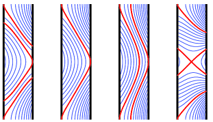
Figure 1: (Color online.) From left to right, the four combinations that are referred to as Fields 1-4 in the text. The thick red lines in each case denote the special field lines across which the linkage to the boundaries changes, and where Shercliff layers are thus expected to arise. The general form is $({\bf\hat{e}}_{z}+c_{I}{\bf B}_{I}+c_{K}{\bf B}_{K})/c_{0}$, where $c_{I}$ and $c_{K}$ are adjusted to select the desired field topology, and $c_{0}$ is then chosen to rescale the maximum amplitude to 1. The precise values of $(c_{I},c_{K})$ are $(0.155,-4.356)$, $(0.124,-3.485)$, $(0.091,-2.562)$, $(0.548,-7.687)$, respectively.

Various linear combinations of ${\bf\hat{e}}_{z}$, ${\bf B}_{I}$ and ${\bf B}_{K}$ then correspond to the linear combinations of dipole and axial fields discussed above. One easily finds that it is possible to construct field line topologies that have no analog in the spherical shell geometry. Fig. 1 shows four possible combinations. In Field 1, there are some field lines that thread only the inner cylinder, some that thread only the outer cylinder, and some that connect the two. Based on the spherical results, if both boundaries are conducting, we would expect to find a super-rotating jet on one dividing line, and a counter-rotating jet on the other. In Field 2, the linear combinations have been adjusted slightly, in such a way that the previously separate dividing field lines coincide, and the region of field lines linking both boundaries has been collapsed to this single line that is tangent to both boundaries, but does not penetrate either. So, what happens in this case, when the previously expected super-rotating and counter-rotating jets should now occur on one and the same field line? In Field 3, the linear combinations have been further adjusted, so there is now a central ribbon of field lines that never touch either boundary, but just continue periodically to $z=\pm\infty$. As with Field 2, this scenario also has no spherical analog, so it is again not clear what to expect in this case. Finally, in Field 4 the linear combinations have been chosen to yield an X-type neutral point in the middle of the domain. This topology is in fact achievable in spherical geometry as well Hollerbach01b , so is included here primarily for completeness and comparison.

We see then that just taking different combinations of ${\bf\hat{e}}_{z}$, ${\bf B}_{I}$ and ${\bf B}_{K}$ already allows us to construct topologies that have no spherical analogs. To all of these we can further add the azimuthal field $r^{-1}{\bf\hat{e}}_{\phi}$, which also has no natural analog in spherical geometry, since it is singular on the $z$-axis, which is part of the domain in spherical geometry but not in cylindrical. Since it is everywhere tangent to the boundaries, this azimuthal field will not alter the fundamental topology of the previously considered fields, but it nevertheless changes the detailed structure of the Shercliff layers that arise on the critical field lines. Indeed, including an azimuthal field component changes the solutions in at least one quite fundamental way: For purely meridional fields, the coupling between the different quantities turns out to be such that in fact $\psi$ and $a$ in Eq. (3) are identically zero (in the $Re\to 0$ limit). Adding an azimuthal component to ${\bf B}_{0}$ introduces new couplings that result in non-zero $\psi$ and $a$. Finally, note also that a purely azimuthal ${\bf B}_{0}$ would not yield any interesting dynamics; the solution in that case is simply the original Couette profile $v=(-r+4r^{-1})/3$, and $\psi=a=b=0$.

To summarize, the goal of this paper is to explore the Shercliff layers that occur on the critical field lines indicated in Fig. 1, either these fields alone or together with azimuthal fields of the form $r^{-1}{\bf\hat{e}}_{\phi}$. This is accomplished by using an axisymmetric, pseudo-spectral code Hollerbach08 to numerically solve Eqs. (1)-(3). Very briefly, $\psi$, $v$, $a$ and $b$ are expanded in terms of Chebyshev polynomials in $r$ and Fourier series in $z$. Eq. (1) is time-stepped until a stationary solution emerges; Eq. (2) is directly inverted for $\bf b$ at each time-step of Eq. (1). Resolutions as large as 240 Chebyshev polynomials and 400 Fourier modes were used, and allow Hartmann numbers as large as $Ha^{2}=10^{7}$ to be achieved.

The associated boundary conditions are no-slip for $\bf U$, and either insulating or perfectly conducting boundaries for $\bf b$, referred to as I and C respectively. Other possible choices could include finitely conducting, or perhaps ferromagnetic, which in other contexts can have a significant influence Gissinger3 . For the Shercliff layer problem the asymptotic analyses Dormy2 ; Mizerski ; Buhler ; Soward indicate that the most relevant parameter is how the conductance of the exterior regions compares with the conductance of the fluid region; if this ratio is small (large) the results are similar to the insulating (perfectly conducting) case. Our I and C choices are therefore natural limiting cases, and even something at first sight quite different, such as ferromagnetic, is likely to be similar to the I case, since they both have zero conductance of the exterior regions.

III Results without imposed $B_{\phi}$

Fig. 2 shows contours of the angular velocity $\omega=v/r$ for the four choices Fields 1-4 alone, without any additional azimuthal component. In every case, the most prominent features are indeed concentrated on the particular field lines singled out in Fig. 1. The contrast between insulating and conducting boundaries is also clear; conducting boundaries exhibit both super-rotation and counter-rotation, especially for Field 4, whereas insulating boundaries only have very weak counter-rotating regions.

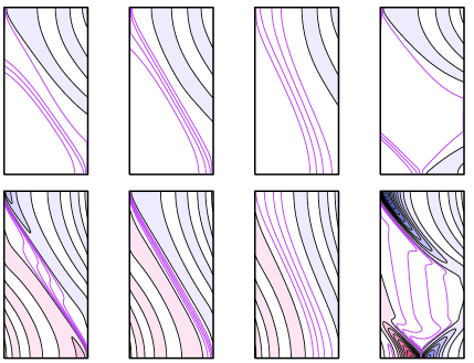
Figure 2: (Color online.) Contours of the angular velocity $\omega=v/r$, for $Ha^{2}=10^{6}$. From left to right are the four choices Fields 1-4. The top row is for insulating boundaries, the bottom row conducting. In each panel only the upper half of the domain is shown; that is, $r$ extends over the full range $[1,2]$, but $z\in[2,4]$. The lower half $z\in[0,2]$ is reflection-symmetric in each case, as seen also in Fig. 1. The white regions indicate values between 0 at the outer boundary and 1 at the inner; the magenta contour lines in these regions have intervals 0.2. The red-shaded regions correspond to super-rotation, where $\omega>1$; the blue-shaded regions correspond to counter-rotation, where $\omega<0$. In both cases the black contour lines in these regions have intervals 1.

In the insulating case there are also Hartmann layers at the boundaries. These layers are so thin, $O(Ha^{-1})$, that they cannot be seen directly at this scale. Their presence can be inferred though by the magenta contour lines, indicating values between 0.2 and 0.8, that appear to touch the boundaries. The actual imposed boundary conditions of course are $\omega=1$ at $r_{i}$ and $\omega=0$ at $r_{o}$, so these contour lines cannot touch the boundaries, and indeed they don’t, but rather remain within the Hartmann layers. These layers were investigated in detail, and always followed the expected $O(Ha^{-1})$ scalings. We therefore concentrate only on the Shercliff layers in the following discussion.

To explore the details of the Shercliff layers, we require more precise diagnostics than the two-dimensional contour plots in Fig. 2. Fig. 3 shows one-dimensional cuts along the midplane $z=2$. Such cuts allow much more quantitative information to be extracted, such as how the thicknesses and amplitudes scale with $Ha$. The thicknesses were again always found to be broadly consistent with the expected $O(Ha^{-1/2})$ scalings. Regarding the amplitudes, insulating boundaries are as expected, with hardly any anomalous rotation for any of Fields 1-4.

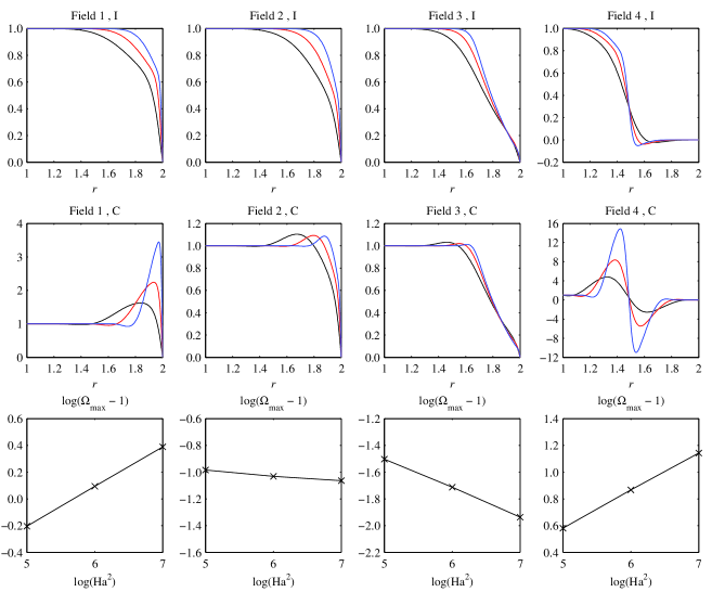
Figure 3: (Color online.) The first two rows show $\omega(r)$ at $z=2$, for Fields 1-4 from left to right as indicated, the first row insulating (I) and the second row conducting (C). Within each panel black-red-blue indicate $Ha^{2}=10^{5}$, $10^{6}$, $10^{7}$, respectively. The third row shows how the amplitude of the super-rotation in the second row scales with $Ha$, and suggests fits of the form $Ha^{s}$, with $s\approx 0.59$, $-0.08$, $-0.43$, $0.56$, respectively.

Conducting boundaries exhibit precisely the features we were expecting, and which make this problem interesting. Starting with Field 1, we see that the super-rotating jet on the field line tangent to the outer boundary is clearly increasing with increasing $Ha$, apparently scaling as $Ha^{0.59}$. The counter-rotating jet on the field line tangent to the inner boundary at $z=4$ has much the same scaling. Similarly for Field 4, we see the same behaviour even more strongly, for both the super-rotating and counter-rotating jets. Field 4 in particular is not only qualitatively, but even quantitatively very similar to corresponding results in spherical geometry – compare for example with Fig. 3 of Hollerbach01b .

In contrast, Field 2 still exhibits a slight super-rotation, but its amplitude seems to be practically independent of $Ha$. Similarly, a cut at $z=4$ has a slight counter-rotation, also with an $Ha$-independent amplitude. We recall that Field 2 is the case where the previously distinct field lines in Field 1 have been made to coincide. Evidently the system adjusts in such a way that weak anomalous rotations remain, but they no longer increase with increasing $Ha$. Finally, for Field 3, having this ribbon of field lines that are not connected to either boundary gives the system so much flexibility in adjusting the shear across the Shercliff layers that the anomalous rotation decreases with increasing $Ha$, apparently scaling as $Ha^{-0.43}$.

To understand the origin of the anomalous rotations, we turn to the Lorentz force $Ha^{2}(\nabla\times{\bf b})\times{\bf B}_{0}$ in Eq. (1). Fig. 4 shows contours of the streamfunction of the induced current $\bf j=\nabla\times b$, for Fields 1 and 3. For both choices, I and C boundaries yield very similar patterns, consisting of clockwise circulation cells. Focusing attention specifically at the point $(r,z)=(2,2)$, the current in all four cases is therefore in the $-{\bf\hat{e}}_{r}$ direction. Since ${\bf B}_{0}$ at this point is in the ${\bf\hat{e}}_{z}$ direction, the Lorentz force will be in the ${\bf\hat{e}}_{\phi}$ direction. It is precisely this force which accelerates the fluid from $\omega=0$ at the boundary to $\omega>0$ in the interior. For insulating boundaries this force is just sufficient to achieve $\omega\approx 1$ on those field lines linked only to the inner boundary, as seen in Figs. 2 and 3.

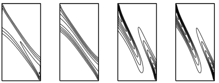
Figure 4: Contours of $b\,r$, which constitutes the streamfunction of the electric current ${\bf j}=\nabla\times(b\,{\bf\hat{e}}_{\phi})$. From left to right Field 1, I and C boundaries, then Field 3, I and C boundaries, and $Ha^{2}=10^{6}$ for all four. All circulation cells are clockwise, with recirculation within the Hartmann boundary layers for the I cases, and through the boundaries for the C cases. As in Fig. 2, only the upper half $z\in[2,4]$ is shown; the circulation cells in the lower half are counter-clockwise. Finally, the contour intervals from left to right are $2\cdot 10^{-4}$, $2\cdot 10^{-3}$, $2\cdot 10^{-5}$ and $3\cdot 10^{-5}$, respectively, and illustrates how switching the boundaries from I to C has a far greater effect for Field 1 than for Field 3.

For conducting boundaries the system essentially ‘over-reacts’, and thereby causes the super-rotation in this region. To understand further why the system over-reacts in this way, we need to consider two (closely related) differences between the insulating and conducting results in Fig. 4. Although the patterns are generally similar for both boundary conditions, in the insulating case the current must recirculate through the Hartmann boundary layers (which are again so thin as to be barely visible here), whereas in the conducting case the current can recirculate through the exterior regions. Recirculating the current is therefore much easier in the conducting case, resulting in a stronger current, hence a stronger Lorentz force, hence the over-reaction. As indicated in Fig. 4, for Field 1 the current is an order of magnitude greater for C than for I boundaries, consistent with the increasing super-rotation, whereas for Field 3 it is only moderately greater, consistent with much weaker, and indeed decreasing super-rotation.

The various other anomalous rotations, at other locations, and also for Fields 2 and 4, are similarly explained by the orientation of the Lorentz force at the position in question. The results for Fields 1 and 4 are fully consistent with the analogous scalings previously obtained in the spherical problem Hollerbach00 ; Hollerbach01 ; Buhler ; Soward . The new cases, Fields 2 and 3, would certainly also merit further asymptotic analyses to discover the precise scalings in these cases, and why they differ from the previous results.

IV Results with imposed $B_{\phi}$

To all the cases studied so far, we now wish to add azimuthal fields of the form $B_{\phi}=\beta r^{-1}{\bf\hat{e}}_{\phi}$, with amplitudes $\beta>0$. This is again a configuration that has not been considered before, but one that fundamentally alters the nature of the $Re\to 0$ ‘pure’ Shercliff layer problem. If ${\bf B}_{0}$ includes an azimuthal component, then the Lorentz force $Ha^{2}(\nabla\times{\bf b})\times{\bf B}_{0}$ in Eq. (1) will include a meridional component, thereby driving a meridional circulation $\nabla\times(\psi\,{\bf\hat{e}}_{\phi})$ that would otherwise be absent. Once $\psi\neq 0$, Eq. (2) will similarly induce a field $\nabla\times(a\,{\bf\hat{e}}_{\phi})$. In the process the previous $v$ and $b$ will also be modified. We will focus especially on how the angular velocity is altered, as well as the new flow component $\nabla\times(\psi\,{\bf\hat{e}}_{\phi})$. We gradually increased $\beta$ from 0, and found that $\beta=O(1)$ is already sufficient to noticeably change the previous results. However, the most significant adjustments seem to occur for somewhat larger values, so we fix $\beta=10$ in the following. (That is, the Hartmann number continues to measure the strength of the imposed meridional field, but the imposed azimuthal field is $\sim 10$ times stronger.)

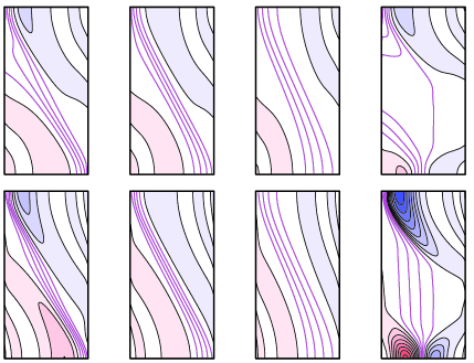
Figure 5: (Color online.) Contours of the angular velocity $\omega=v/r$, for $Ha^{2}=10^{6}$, and with $B_{\phi}=10r^{-1}{\bf\hat{e}}_{\phi}$ added to the previous choices Fields 1-4. All eight panels are exactly as in Fig. 2, except that the contour interval is now 0.2 throughout, for both the magenta and the black contour lines.

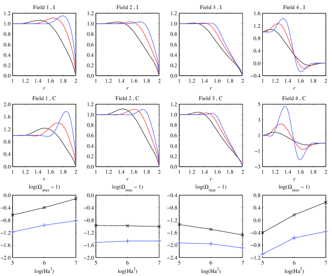
Figure 6: (Color online.) As in Fig. 3, the first two rows show $\omega(r)$ at $z=2$, for Fields 1-4 and I and C as indicated. Within each panel black-red-blue again corresponds to $Ha^{2}=10^{5}$, $10^{6}$, $10^{7}$. In the third row, the blue lines ($+$ symbols) and the black lines ($\times$ symbols) show the scalings with $Ha$ of the I and C super-rotations, respectively.

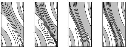
Figure 7: Contours of $\psi\,r$, which constitutes the streamfunction of the meridional circulation $\nabla\times(\psi\,{\bf\hat{e}}_{\phi})$. From left to right Field 1, I and C boundaries, then Field 3, I and C boundaries, and $Ha^{2}=10^{6}$ for all four. White indicates negative values, grey positive. The contour intervals are $5\cdot 10^{-3}$ for Field 1, and $10^{-3}$ for Field 3.

Fig. 5 shows the equivalent of Fig. 2. The qualitative features are still similar, but there are also clear differences. Most notably, the very strong anomalous rotations in the conducting case have been substantially reduced. All of the various Shercliff layers also seem to be considerably thicker than before, although an examination of the variation with $Ha$ still suggests a scaling as $O(Ha^{-1/2})$.

Fig. 6 again shows cuts at $z=2$. Comparing with Fig. 3, the key differences are: (a) the broadening of the Shercliff layers already noted above, (b) the presence of anomalous rotation in the I case, (c) the strong suppression of anomalous rotation in the C case, and (d) the broadly similar scalings of the anomalous rotations in the I and C cases. We note though that the anomalous rotation scalings in most cases are not as clear as in Fig. 3; for Fields 1-3 one might conjecture scalings roughly as $s\approx 0.45$, $0.0$ and $-0.3$, respectively, but for Field 4 one probably should not speculate about a particular exponent at all.

Finally, Fig. 7 shows examples of the meridional circulation. As one might expect, it also tends to align with the previously existing Shercliff layers, which continue to dominate the flow, that is, $U_{\phi}\gg U_{z},\,U_{r}$. For both choices of imposed field the I and C options also yield broadly similar magnitudes of $\psi$.

We conclude this section, and this paper, by noting that while the $\beta>0$ case yields Shercliff layers similar in many ways to the previously studied $\beta=0$ case, there are also clear differences, and many of the precise scalings are almost certainly different. An asymptotic analysis of this problem along the lines of the previous analyses Dormy2 ; Mizerski ; Buhler ; Soward would be of considerable interest.

V Acknowledgments

DH’s visit to Leeds was supported by an Erasmus+ scholarship and by ‘Region Stages mobilité’ from Haute-Normandie.

References

- (1) J.A. Shercliff, The flow of conducting fluids in circular pipes under transverse magnetic fields, J. Fluid Mech. 1 (1956) 644–666.
- (2) E. Dormy, P. Cardin, D. Jault, MHD flow in a slightly differentially rotating spherical shell, with conducting inner core, in a dipolar magnetic field, Earth Planet. Sci. Lett. 160 (1998) 15–30.
- (3) S.V. Starchenko, Magnetohydrodynamic flow between insulating shells rotating in strong potential field, Phys. Fluids 10 (1998) 2412–2420.
- (4) P.H. Roberts, Singularities of Hartmann layers, Proc. Royal Soc. A 300 (1967) 94–107.
- (5) R. Hollerbach, Magnetohydrodynamic flows in spherical shells, in: C. Egbers, G. Pfister (Eds.), Physics of Rotating Fluids, Springer, 2000.
- (6) R. Hollerbach, S. Skinner, Instabilities of magnetically induced shear layers and jets, Proc. Royal Soc. A 457 (2001) 785–802.
- (7) E. Dormy, D. Jault, A.M. Soward, A super-rotating shear layer in magnetohydrodynamic spherical Couette flow, J. Fluid Mech. 452 (2002) 263–291.
- (8) K.A. Mizerski, K. Bajer, On the effect of mantle conductivity on the super-rotating jets near the liquid core surface, Phys. Earth Planet. Inter. 160 (2007) 245-268.
- (9) L. Bühler, On the origin of super-rotating layers in magnetohydrodynamic flows, Theoret. Comput. Fluid Dynam. 23 (2009) 491–507.
- (10) A.M. Soward, E. Dormy, Shear-layers in magnetohydrodynamic spherical Couette flow with conducting walls, J. Fluid Mech. 645 (2010) 145–185.
- (11) R. Hollerbach, Super- and counter-rotating jets and vortices in strongly magnetic spherical Couette flow, in: P. Chossat, D. Armbruster, J. Oprea (Eds.), Dynamo and Dynamics, a Mathematical Challenge, Springer, 2001.
- (12) H.-C. Nataf, T. Alboussiere, D. Brito, P. Cardin, N. Gagniere, D. Jault, J.-P. Masson, D. Schmitt, Experimental study of super-rotation in a magnetostrophic spherical Couette flow, Geophys. Astrophys. Fluid Dynam. 100 (2006) 281–298.
- (13) D. Brito, T. Alboussiere, P. Cardin, N. Gagniere, D. Jault, P. La Rizza, J.-P. Masson, H.-C. Nataf, D. Schmitt, Zonal shear and super-rotation in a magnetized spherical Couette-flow experiment, Phys. Rev. E 83 (2011) 066310.
- (14) S. Cabanes, N. Schaeffer, H.-C. Nataf, Magnetic induction and diffusion mechanisms in a liquid sodium spherical Couette experiment, Phys. Rev. E 90 (2014) 043018.
- (15) D.R. Sisan, N. Mujica, W.A. Tillotson, Y.M. Huang, W. Dorland, A.B. Hassam, T.M. Antonsen, D.P. Lathrop, Experimental observation and characterization of the magnetorotational instability, Phys. Rev. Lett. 93 (2004) 114502.
- (16) D.S. Zimmerman, S.A. Triana, H.-C. Nataf, D.P. Lathrop, A turbulent, high magnetic Reynolds number experimental model of Earth’s core, J. Geophys. Res. Solid Earth 119 (2014) 4538–4557.
- (17) E.J. Spence, A.H. Roach, E.M. Edlund, P. Sloboda, H. Ji, Free magnetohydrodynamic shear layers in the presence of rotation and magnetic field, Phys. Plasmas 19 (2012) 056502.
- (18) A.H. Roach, E.J. Spence, C. Gissinger, E.M. Edlund, P. Sloboda, J. Goodman, H.T. Ji, Observation of a free Shercliff layer instability in cylindrical geometry, Phys. Rev. Lett. 108 (2012) 154502.
- (19) Z. Stelzer, D. Cebron, S. Miralles, S. Vantieghem, J. Noir, P. Scarfe, A. Jackson, Experimental and numerical study of electrically driven magnetohydrodynamic flow in a modified cylindrical annulus. I. Base flow, Phys. Fluids 27 (2015) 077101.
- (20) Z. Stelzer, S. Miralles, D. Cebron, J. Noir, S. Vantieghem, A. Jackson, Experimental and numerical study of electrically driven magnetohydrodynamic flow in a modified cylindrical annulus. II. Instabilities, Phys. Fluids 27 (2015) 084108.
- (21) R. Hollerbach, E. Canet, A. Fournier, Spherical Couette flow in a dipolar magnetic field, Eur. J. Mech. B 26 (2007) 729–737.
- (22) R. Hollerbach, Non-axisymmetric instabilities in magnetic spherical Couette flow, Proc. Royal Soc. A 465 (2009) 2003–2013.
- (23) C. Gissinger, H. Ji, J. Goodman, Instabilities in magnetized spherical Couette flow, Phys. Rev. E 84 (2011) 026308.
- (24) C. Gissinger, J. Goodman, H. Ji, The role of boundaries in the magnetorotational instability, Phys. Fluids 24 (2012) 074109.
- (25) A. Figueroa, N. Schaeffer, H.-C. Nataf, D. Schmitt, Modes and instabilities in magnetized spherical Couette flow, J. Fluid Mech. 716 (2013) 445–469.
- (26) H.-C. Nataf, Magnetic induction maps in a magnetized spherical Couette flow experiment, Comptes Rendus Phys. 14 (2013) 248–267.
- (27) E.J. Kaplan, Saturation of nonaxisymmetric instabilities of magnetized spherical Couette flow, Phys. Rev. E 89 (2014) 063016.
- (28) G. Rüdiger, L.L. Kitchatinov, R. Hollerbach, Magnetic Processes in Astrophysics: Theory, Simulations, Experiments, Wiley-VCH, 2013.
- (29) M. Abramowitz, I.A. Stegun, Handbook of Mathematical Functions, Dover, 1968.
- (30) R. Hollerbach, Spectral solutions of the MHD equations in cylindrical geometry, Int. J. Pure Appl. Math. 42 (2008) 575–581.
- (31) C. Gissinger, A. Iskakov, S. Fauve, E. Dormy, Effect of magnetic boundary conditions on the dynamo threshold of von Kármán swirling flows, EPL 82 (2008) 29001.