An Online Hierarchical Algorithm for Extreme Clustering

Abstract

Many modern clustering methods scale well to a large number of data items, $N$, but not to a large number of clusters, $K$. This paper introduces Perch, a new non-greedy algorithm for online hierarchical clustering that scales to both massive $N$ and $K$—a problem setting we term extreme clustering. Our algorithm efficiently routes new data points to the leaves of an incrementally-built tree. Motivated by the desire for both accuracy and speed, our approach performs tree rotations for the sake of enhancing subtree purity and encouraging balancedness. We prove that, under a natural separability assumption, our non-greedy algorithm will produce trees with perfect dendrogram purity regardless of online data arrival order. Our experiments demonstrate that Perch constructs more accurate trees than other tree-building clustering algorithms and scales well with both $N$ and $K$, achieving a higher quality clustering than the strongest flat clustering competitor in nearly half the time.

1 Introduction

Clustering algorithms are a crucial component of any data scientist’s toolbox with applications ranging from identifying themes in large text corpora [11], to finding functionally similar genes [18], to visualization, pre-processing, and dimensionality reduction [22]. As such, a number of clustering algorithms have been developed and studied by the statistics, machine learning, and theoretical computer science communities. These algorithms and analyses target a variety of scenarios, including large-scale, online, or streaming settings [39, 2], clustering with distribution shift [3], and many more.

Modern clustering applications require algorithms that scale gracefully with dataset size and complexity. In clustering, data set size is measured by the number of points $N$ and their dimensionality $d$, while the number of clusters, $K$, serves as a measure of complexity. While several existing algorithms can cope with large datasets, very few adequately handle datasets with many clusters. We call problem instances with large $N$ and large $K$ extreme clustering problems–a phrase inspired by work in extreme classification [13].

Extreme clustering problems are increasingly prevalent. For example, in entity resolution, record linkage and deduplication, the number of clusters (i.e., entities) increases with dataset size [7] and can be in the millions. Similarly, the number of communities in typical real world networks tends to follow a power-law distribution [14] that also increases with network size. Although used primarily in classification tasks, the ImageNet dataset also describes precisely this large $N$, large $K$ regime ($N\approx 14$M,$K\approx 21$K) [17, 34].

This paper presents a new online clustering algorithm, called Perch, that scales mildly with both $N$ and $K$ and thus addresses the extreme clustering setting. Our algorithm constructs a tree structure over the data points in an incremental fashion by routing incoming points to the leaves, growing the tree, and maintaining its quality via simple rotation operations. The tree structure enables efficient (often logarithmic time) search that scales to large datasets, while simultaneously providing a rich data structure from which multiple clusterings at various resolutions can be extracted. The rotations provide an efficient mechanism for our algorithm to recover from mistakes that arise with greedy incremental clustering procedures.

Operating under a simple separability assumption about the data, we prove that our algorithm constructs a tree with perfect dendrogram purity regardless of the number of data points and without knowledge of the number of clusters. This analysis relies crucially on a recursive rotation procedure employed by our algorithm. For scalability, we introduce another flavor of rotations that encourage balancedness, and an approximation that enables faster point insertions. We also develop a leaf collapsing mode of our algorithm that can operate in memory-limited settings, when the dataset does not fit in main memory.

We empirically demonstrate that our algorithm is both accurate and efficient for a variety of real world data sets. In comparison to other tree-building algorithms (that are both online and multipass), Perch achieves the highest dendrogram purity in addition to being efficient. When compared to flat clustering algorithms where the number of clusters is given by an oracle, Perch with a pruning heuristic outperforms or is competitive with all other scalable algorithms. In both comparisons to flat and tree building algorithms, Perch scales best with the number of clusters $K$.

2 The Clustering Problem

In a clustering problem we are given a dataset $X=\{x_{i}\}_{i=1}^{N}$ of points. The goal is to partition the dataset into a set of disjoint subsets (i.e., clusters), $\mathcal{C}$, such that the union of all subsets covers the dataset. Such a set of subsets is called a clustering. A high quality clustering is one in which the points in any particular subset are more similar to each other than the points in other subsets.

A clustering, $\mathcal{C}$, can be represented as a map from points to clusters identities, $\mathcal{C}:X\to\{1,\ldots,K\}$. However, structures that encode more fine-grained information also exist. For example, prior works construct a cluster tree over the dataset to compactly encode multiple alternative tree-consistent partitions, or clusterings [23, 9].

Definition 1 (Cluster tree [25]).

A binary cluster tree $\mathcal{T}$ on a dataset $\{x_{i}\}_{i=1}^{N}$ is a collection of subsets such that $C_{0}\triangleq\{x_{i}\}_{i=1}^{N}\in\mathcal{T}$ and for each $C_{i},C_{j}\in\mathcal{T}$ either $C_{i}\subset C_{j}$, $C_{j}\subset C_{i}$ or $C_{i}\cap C_{j}=\emptyset$. For any $C\in\mathcal{T}$, if $\exists C^{\prime}\in\mathcal{T}$ with $C^{\prime}\subset C$, then there exists two $C_{L},C_{R}\in\mathcal{T}$ that partition $C$.

Given a cluster tree, each internal node can be associated with a cluster that includes its descendant points. A tree-consistent partition is a subset of the nodes in the tree whose associated clusters partition the dataset, and hence is a valid clustering.

Cluster trees afford multiple advantages in addition to their representational power. For example, when building a cluster tree it is typically unnecessary to specify the number of target clusters (which, in virtually all real-world problems, is unknown). Cluster trees also provide the opportunity for efficient cluster assignment and search, which is particularly important for large datasets with many clusters. In such problems, $O(K)$ search required by classical methods can be prohibitive, while a top down traversal of a cluster tree could offer $O(\log(K))$ search, which is exponentially faster.

Evaluating a cluster tree is more complex than evaluating a flat clustering. Assuming that there exists a ground truth clustering $\mathcal{C}^{\star}=\{C_{k}^{\star}\}_{i=1}^{K}$ into $K$ clusters, it is common to measure the quality of a cluster tree based on a single clustering extracted from the tree. We follow Heller et. al and adopt a more holistic measure of the tree quality, known as dendrogram purity [23]. Define

$$\mathcal{P}^{\star}=\{(x_{i},x_{j})\mid\mathcal{C}^{\star}(x_{i})=\mathcal{C}^{\star}(x_{j})\}$$

to be the pairs of points that are clustered together in the ground truth. Then, dendrogram purity is defined as follows:

Definition 2 (Dendrogram Purity).

Given a cluster tree $\mathcal{T}$ over a dataset $X=\{x_{i}\}_{i=1}^{N}$, and a true clustering $\mathcal{C}^{\star}$, the dendrogram purity of $\mathcal{T}$ is

$$\texttt{DP}(\mathcal{T})=\frac{1}{|\mathcal{P}^{\star}|}\sum_{k=1}^{K}\sum_{x_{i},x_{j}\in\mathcal{C}^{\star}_{k}}\texttt{pur}(\texttt{lvs}(\texttt{LCA}(x_{i},x_{j})),\mathcal{C}^{\star}_{k})$$

where $\texttt{LCA}(x_{i},x_{j})$ is the least common ancestor of $x_{i}$ and $x_{j}$ in $\mathcal{T}$, $\texttt{lvs}(z)\subset X$ is the set of leaves for any internal node $z$ in $\mathcal{T}$, and pur$(S_{1},S_{2})=|S_{1}\cap S_{2}|/|S_{1}|$.

In words, the dendrogram purity of a tree with respect to a ground truth clustering is the expectation of the following random process: (1) sample two points, $x_{i},\ x_{j}$, uniformly at random from the pairs in the ground truth (and thus $\mathcal{C}^{\star}(x_{i})=\mathcal{C}^{\star}(x_{j})$), (2) compute their least common ancestor in ${\mathcal{T}}$ and the cluster (i.e. descendant leaves) of that internal node, (3) compute the fraction of points from this cluster that also belong to $\mathcal{C}^{\star}(x_{i})$. For large-scale problems, we use Monte Carlo approximations of dendrogram purity. More intuitively, dendrogram purity obviates the (often challenging) task of extracting the best tree-consistent partition, while still providing a meaningful measure of overlap with the ground truth flat clustering.

3 Tree Construction

Our work is focused on instances of the clustering problem in which the size of the dataset $N$ and the number of clusters $K$ are both very large. In light of their advantages with respect to efficiency and representation (Section 2), our method builds a cluster tree over data points. We are also interested in the online problem setting–in which data points arrive one at a time–because this resembles real-world scenarios in which new data is constantly being created. Well-known clustering methods based on cluster trees, like hierarchical agglomerative clustering, are often not online; there exist a few online cluster tree approaches, most notably BIRCH [39], but empirical results show that BIRCH typically constructs worse clusterings than most competitors [29, 2].

The following subsections describe and analyze several fundamental components of our algorithm, which constructs a cluster tree in an online fashion. The data points are assumed to reside in Euclidean space: $\{x_{i}\}_{i=1}^{N}\subset\mathbb{R}^{d}$. We make no assumptions on the order in which the points are processed.

3.1 Preliminaries

In the clustering literature, it is common to make various separability assumptions about the data being clustered. As one example, a set of points is $\epsilon$-separated for K-means if the ratio of the clustering cost with $K$ clusters to the cost with $K-1$ clusters is less than $\epsilon^{2}$ [31]. While assumptions like these generally do not hold in practice, they motivate the derivation of several powerful and justifiable algorithms. To derive our algorithm, we make a strong separability assumption under $\mathcal{C}^{\star}$.

Assumption 1 (Separability).

A data set $X$ is separable with respect to a clustering $\mathcal{C}^{\star}$ if

$$\max_{(x,y)\in\mathcal{P}^{\star}}\|x-y\|<\min_{(x^{\prime},y^{\prime})\notin\mathcal{P}^{\star}}\|x^{\prime}-y^{\prime}\|,$$

where $\|\cdot\|$ is the Euclidean norm. We assume that $X$ is separable with respect to $\mathcal{C}^{\star}$.

Thus under separability, the true clustering has all within-cluster distances smaller than any between-cluster distance. The assumption is quite strong, but it is not without precedent. As just one example, the NCBI uses a form of separability in their clique-based approach for protein clustering [33]. Moreover, separability aligns well with existing clustering methods; for example under separability, agglomerative methods like complete, single, and average linkage are guaranteed to find $\mathcal{C}^{\star}$, and $\mathcal{C}^{\star}$ is guaranteed to contain the unique optimum of the $K$-center cost function. Lastly, we use separability primarily for theoretically grounding the design of our algorithm, and we do not expect it to hold in practice. Our empirical analysis shows that our algorithm outperforms existing methods even without separability assumptions.

3.2 The Greedy Algorithm and Masking

The derivation of our algorithm begins from an attempt to remedy issues with greedy online tree construction. Consider the following greedy algorithm: when processing point $x_{i}$, a search is preformed to find its nearest neighbor in the current tree. The search returns a leaf node, $\ell$, containing the nearest neighbor of $x_{i}$. A Split operation is performed on $\ell$ that: (1) disconnects $\ell$ from its parent, (2) creates a new leaf $\ell^{\prime}$ that stores $x_{i}$, (3) creates a new internal node whose parent is $\ell$’s former parent and with children $\ell$ and $\ell^{\prime}$.

Fact 1.

There exists a separable clustering instance in $1$-dimension with two balanced clusters where the greedy algorithm has dendrogram purity at most $7/8$.

Proof.

The construction has two clusters, one with half its points near $-1$ and half its points near $+1$, and another with all points around $+4$, so the instance is separable. If we show one point near $-1$, one point near $+1$, and then a point near $+4$, one child of the root contains the latter two points, so the true clustering is irrecoverable. To calculate the purity, notice that at least $1/2$ of the pairs from cluster one have the root as the LCA, so their purity is $1/2$ and the total dendrogram purity is at most $7/8$. ∎

It is easy to generalize the construction to more clusters and higher dimension, although upper bounding the dendrogram purity may become challenging. The impurity in this example is a result of the leaf at $+1$ becoming masked when $+4$ is inserted.

Definition 3 (Masking).

A node $v$ with sibling $v^{\prime}$ and aunt $a$ in a tree ${\mathcal{T}}$ is masked if there exists a point $x\in\texttt{lvs}(v)$ such that

$$\max_{y\in\texttt{lvs}(v^{\prime})}\|x-y\|>\min_{z\in\texttt{lvs}(a)}\|x-z\|.$$ (1)

Thus, $v$ contains a point $x$ that is closer to some point in the aunt $a$ than some point in the sibling $v^{\prime}$. Intuitively, masking happens when a point is misclustered. For example when a point belonging to the same cluster as $v$’s leaves is sent to $a$, then $v$ becomes masked. A direct child of the root cannot be masked since it has no aunt.

Under separability, masking is intimately related to dendrogram purity, as demonstrated in the following result.

Fact 2.

If $X$ is separated w.r.t. $\mathcal{C}^{\star}$and a cluster tree $\mathcal{T}$ contains no masked nodes, then it has dendrogram purity 1.

Proof.

Assume that ${\mathcal{T}}$ does not have dendrogram purity 1. Then there exists points $x_{i}$ and $x_{j}$ in $\texttt{lvs}({\mathcal{T}})$ such that $\mathcal{C}^{\star}(x_{i})=\mathcal{C}^{\star}(x_{j})$ but $\texttt{lvs}(\texttt{LCA}(x_{i},x_{j}))$ contains a point $x_{k}$ in a different cluster. The least common ancestor has two children $v_{\ell},v_{r}$ and $x_{i},x_{j}$ cannot be in the same child, so without loss of generality we have $x_{i},x_{k}\in v_{l}$ and $x_{j}\in v_{r}$. Now consider $v=\texttt{LCA}(x_{i},x_{k})$ and $v$’s sibling $v^{\prime}$. If $v^{\prime}$ contains a point belonging to $\mathcal{C}^{\star}(x_{i})$, then the child of $v$ that contains $x_{i}$ is masked since $x_{i}$ is closer to that point than it is to $x_{k}$. If the aunt of $v$ contains a point belonging to $\mathcal{C}^{\star}(x_{i})$ then $v$ is masked for the same reason. If the aunt contains only points that do not belong to $\mathcal{C}^{\star}(x_{i})$ then examine $v$’s parent and proceed recursively. This process must terminate since we are below $\texttt{LCA}(x_{i},x_{j})$. Thus the leaf containing $x_{i}$ or one of $x_{i}$’s ancestors must be masked. ∎

3.3 Masking Based Rotations

Inspired by self-balancing binary search trees [36], we employ a novel masking-based rotation operation that alleviates purity errors caused by masking. In the greedy algorithm, after inserting a new point as leaf $\ell^{\prime}$ with sibling $\ell$, the algorithm checks if $\ell$ is masked. If masking is detected, a Rotate operation is performed, which swaps the positions of $\ell^{\prime}$ and its aunt in the tree (See Figure 1). After the rotation, the algorithm checks if $\ell$’s new sibling is masked and recursively applies rotations up the tree. If no masking is detected at any point in the process, the algorithm terminates.

At this point in the discussion, we check for masking exhaustively via Equation (1). In the next section we introduce approximations for scalability.

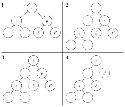
Figure 1: The Rotate procedure in four steps. In each step, the change to the tree is indicated by dotted lines.

Theorem 1.

If $X$ is separated w.r.t. $\mathcal{C}^{\star}$, the greedy algorithm with masking-based rotations constructs a cluster tree with dendrogram purity 1.0.

Proof Sketch.

Inductively, assume our current cluster tree $\mathcal{T}$ has dendrogram purity 1.0, and we process a new point $x_{i}$ belonging to ground truth cluster $C^{\star}\in\mathcal{C}^{\star}$. In the first case, assume that $\mathcal{T}$ already contains some members of $C^{\star}$ that are located in a (pure) subtree, ${\mathcal{T}}[C^{\star}]$. Then, by separability $x_{i}$’s nearest neighbor must be in ${\mathcal{T}}[C^{\star}]$ and if rotations ensue, no internal node $v\in{\mathcal{T}}[C^{\star}]$ can be rotated outside of $T[C^{\star}]$. To see why, observe that the children of ${\mathcal{T}}[C^{\star}]$’s root cannot be masked since this is a pure subtree and before insertion of $v$ the full tree itself was pure (so no points from $C^{\star}$ can be outside of ${\mathcal{T}}[C^{\star}]$). In the second case, assume that $T$ contains no points from cluster $C^{\star}$. Then, again by separability, recursive rotations must lift $x_{i}$ out of the pure subtree that contains its nearest neighbor, which allows $\mathcal{T}$ to maintain perfect purity. ∎

4 Scaling

Two sub-procedures of the algorithm described above can render its naive implementation slow: finding nearest neighbors and checking whether a node is masked. Therefore, in this section we introduce several approximations that make our final algorithm, Perch, scalable. First, we describe a balance-based rotation procedure that helps to balance the tree and makes insertion of new points much faster. Then we discuss a collapsed mode that allows our algorithm to scale to datasets that do not fit in memory. Finally, we introduce a bounding-box approximation that makes both nearest neighbor and masking detection operations efficient.

4.1 Balance Rotations

While our rotation algorithm (Section 3.3) guarantees optimal dendrogram purity in the separable case, it does not make any guarantees on the depth of the tree, which influences the running time. Naturally, we would like to construct balanced binary trees, as these lead to logarithmic time search and insertion. We use the following notion of balance.

Definition 4 (Cluster Tree Balance).

The balance of a cluster tree ${\mathcal{T}}$, denoted $\texttt{bal}(\mathcal{T})$, is the average local balance of all nodes in ${\mathcal{T}}$, where the local balance of a node $v$ with children $v_{\ell},v_{r}$ is $\texttt{bal}(v)=\frac{\min\{|\texttt{lvs}(v_{\ell})|,|\texttt{lvs}(v_{r})|\}}{\max\{|\texttt{lvs}(v_{\ell})|,|\texttt{lvs}(v_{r})|\}}$.

To encourage balanced trees, we use a balance-based rotation operation. A balance-rotation with respect to a node $v$ with sibling $v^{\prime}$ and aunt $a$ is identical to a masking-based rotation with respect to $v$, except that it is triggered when

• the rotation would produce a tree ${\mathcal{T}}^{\prime}$ with $\texttt{bal}({\mathcal{T}}^{\prime})>\texttt{bal}({\mathcal{T}})$; and

• there exists a point $x_{i}\in\texttt{lvs}(v)$ such that $x_{i}$ is closer to a leaf of $a$ than to some leaf of $v^{\prime}$ (i.e. Equation (1) holds).

Under separability, this latter check ensures that the balance-based rotation does not compromise dendrogram purity.

Fact 3.

Let $X$ be a dataset that is separable w.r.t $\mathcal{C}^{\star}$. If ${\mathcal{T}}$ is a cluster tree with dendrogram purity 1 and ${\mathcal{T}}^{\prime}$ is the result of a balance-based rotation on some node in ${\mathcal{T}}$, then $\texttt{bal}({\mathcal{T}}^{\prime})>\texttt{bal}({\mathcal{T}})$ and ${\mathcal{T}}^{\prime}$ also has dendrogram purity 1.0.

Proof.

The only situation in which a rotation could impact the dendrogram purity of a pure cluster tree ${\mathcal{T}}$ is when $v$ and $v^{\prime}$ belong to the same cluster, but their aunt $a$ belongs to a different cluster. In this case, separation ensures that

$$\max_{x\in\texttt{lvs}(v),y\in\texttt{lvs}(v^{\prime})}\|x-y\|\leq\min_{x^{\prime}\in\texttt{lvs}(v),z\in\texttt{lvs}(a)}\|x^{\prime}-z\|,$$

so a rotation will not be triggered. Clearly, $\texttt{bal}({\mathcal{T}}^{\prime})>\texttt{bal}({\mathcal{T}})$ since it is explicitly checked before performing a rotation. ∎

After inserting a new point and applying any masking-based rotations, we check for balance-based rotations at each node along the path from the newly created leaf to the root.

4.2 Collapsed Mode

For extremely large datasets that do not fit in memory, we use a collapsed mode of Perch. In this mode, the algorithm takes a parameter that is an upper bound on the number of leaves in the cluster tree, which we denote with $L$. After balance rotations, our algorithm invokes a Collapse procedure that merges leaves as necessary to meet the upper bound. This is similar to work in hierarchical extreme classification in which the depth of the model is a user-specified parameter [15].

The Collapse operation may only be invoked on an internal node $v$ whose children are both leaves. The procedure makes $v$ a collapsed leaf that stores the (ids, not the features, of the) points associated with its children along with sufficient statistics (Section 4.3), and then deletes both children. The points stored in a collapsed leaf are never split by any flavor of rotation. The Collapse operation may be invoked on internal nodes whose children are collapsed leaves.

When the cluster tree has $L+1$ leaves, we collapse the node whose maximum distance between children is minimal among all collapsible nodes, and we use a priority queue to amortize the search for this node. Collapsing this node is guaranteed to preserve dendrogram purity in the separable case.

Fact 4.

Let $X$ be a dataset separable w.r.t. $\mathcal{C}^{\star}$ which has $K$ clusters, if $L>K$, then collapse operations preserve perfect dendrogram purity.

Proof.

Inductively, assume that the cluster tree has dendrogram purity 1.0 before we add a point that causes us to collapse a node. Since $L>K$ and all subtrees are pure, by the pigeonhole principle, there must be a pure subtree containing at least $2$ points. By separability, all such pure $2$-point subtrees will be at the front of the priority queue, before any impure ones, and hence the collapse will not compromise purity. ∎

Algorithm 1 Insert$(x_{i},{\mathcal{T}})$

  $t=$ NearestNeighbor$(x_{i})$

  $l=$ Split$(t)$

  for $a$ in Ancestors$(l)$ do

     $a.$AddPt$(x_{i})$

  end for

  $T=T.\texttt{RotateRec}(\ell.\texttt{Sibling}(),\texttt{CheckMasked})$

  $T=T.\texttt{RotateRec}(\ell.\texttt{Sibling}(),\texttt{CheckBalanced})$

  if CollapseMode then

     $T.\texttt{TryCollapse()}$.

  end if

  Output: $T$

Algorithm 2 RotateRec$(v,{\mathcal{T}},\texttt{func})$

  (ShouldRotate,ShouldStop) = $\texttt{func}(v)$

  if ShouldRotate then

     $T.\texttt{Rotate}(v)$

  end if

  if ShouldStop then

     Output: ${\mathcal{T}}$

  else

     Output: ${\mathcal{T}}.\texttt{RotateRec}(v.\texttt{Parent}(),{\mathcal{T}},\texttt{func})$

  end if

4.3 Bounding Box Approximations

Many of the operations described thus far depend on nearest neighbor searches, which in general can be computationally intensive. We alleviate this complexity by approximating a set (or subtree) of points via a bounding box. Here each internal node maintains a bounding box that contains all of its leaves. Bounding boxes are easy to maintain and update in $\mathcal{O}(d)$ time.

Specifically, for any internal node $v$ whose bounding interval in dimension $j$ is $[v_{-}(j),v_{+}(j)]$, we approximate the squared minimum distance between a point $x$ and $\texttt{lvs}(v)$ by

$$d_{-}(x,v)^{2}=\sum_{j=1}^{d}\left\{\begin{aligned} &(x(j)-v_{-}(j))^{2}&\textrm{if }x(j)\leq v_{-}(j)\\ &(x(j)-v_{+}(j))^{2}&\textrm{if }x(j)\geq v_{+}(j)\\ &0&\textrm{otherwise}\end{aligned}\right.$$ (2)

We approximate the squared maximum distance by

$$d_{+}(x,v)^{2}=\sum_{j=1}^{d}\max\left\{(x(j)-v_{-}(j))^{2},(x(j)-v_{+}(j))^{2}\right\}.$$ (3)

It is easy to verify that these provide lower and upper bounds on the squared minimum and maximum distance between $x$ and $\texttt{lvs}(v)$. See Figure 2 for a visual representation.

For the nearest neighbor search involved in inserting a point $x$ into $\mathcal{T}$, we use the minimum distance approximation $d_{-}(x,v)$ as a heuristic in $A^{\star}$ search. Our implementation maintains a frontier of unexplored internal nodes of $\mathcal{T}$ and repeatedly expands the node $v$ with minimal $d_{-}(x,v)$ by adding its children to the frontier. Since the approximation $d_{-}$ is always a lower bound and it is exact for leaves, it is easy to see that the first leaf visited by the search is the nearest neighbor of $x$. This is similar to the nearest neighbor search in the Balltree data structure [30].

For masking rotations, we use a more stringent check based on Equation 1. Specifically, we perform a masking rotation on node $v$ with sibling $v^{\prime}$ and aunt $a$ if:

$$d_{-}(v,v^{\prime})>d_{+}(v,a)$$ (4)

Note that $d_{-}(v,v^{\prime})$ is a slight abuse of notation (and so is $d_{+}(v,a)$) because both $v$ and $v^{\prime}$ are bounding boxes. To compute, $d_{-}(v,v^{\prime})$, for each dimension in $v$’s bounding box, use either the minimum or maximum along that dimension to minimize the sum of coordinate-wise distances (Equation 2). A similar procedure can be performed to compute $d_{+}(v,a)$ between two bounding boxes.

Note that if Equation 4 holds then $v$ is masked and a rotation with respect to $v$ will unmask $v$ because, for all $x\in\texttt{lvs}(v)$:

$$\max_{y\in\texttt{lvs}(v^{\prime})}||x-y|| \geq\min_{y\in\texttt{lvs}(v^{\prime})}||x-y|| \geq d_{-}(v,v^{\prime})\geq d_{+}(v,a) \geq\max_{z\in\texttt{lvs}(a)}||x-z|| \geq\min_{z\in\texttt{lvs}(a)}||x-z||.$$

In words, we know that rotation will unmask $v$ because the upper bound on the distance from a point in $v$ to a point in $a$ is smaller than the lower bound on the distance from a point in $v$ to a point in $v^{\prime}$.

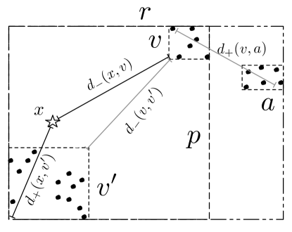
Figure 2: A subtree $r$ with two children $p$ and $a$; $p$ is the parent of $v$ and $v^{\prime}$ (all nodes indicated by boxes with dashed outlines). A point $x$ is inserted and descends to $v^{\prime}$ because $d_{+}(x,v^{\prime})<d_{-}(x,v)$ (black lines). The node $v$ is masked because $d_{+}(v,a)<d_{-}(v,v^{\prime})$ (gray lines).

5 Perch

Our algorithm is called Perch, for Purity Enhancing Rotations for Cluster Hierarchies.

Perch can be run in several modes. All modes use bounding box approximations, masking-, and balance-based rotations. The standard implementation, simply denoted Perch, only includes these features (See Algorithm 2). Perch-C additionally runs in collapsed mode and requires the parameter $L$ for the maximum number of leaves. Perch-B replaces the A^⋆ search with a breadth-first beam search to expedite the nearest neighbor lookup. This mode also takes the beam width as a parameter. Finally Perch-BC uses both the beam search and runs in collapsed mode.

We implement Perch to mildly exploit parallelism. When finding nearest neighbors via beam or A^⋆ search, we use multiple threads to expand the frontier in parallel.

6 Experiments

We compare Perch to several state-of-the-art clustering algorithms on large-scale real-world datasets. Since few benchmark clustering datasets exhibit a large number of clusters, we conduct experiments with large-scale classification datasets that naturally contain many classes and simply omit the class labels. Note that other work in large-scale clustering recognizes this deficiency with the standard clustering benchmarks [7, 4]. Although smaller datasets are not our primary focus, we also measure the performance of Perch on standard clustering benchmarks.

6.1 Experimental Details

Algorithms.

We compare the following 10 clustering algorithms:

• Perch - Our algorithm, we use several of the various modes depending on the size of the problem. For beam search, we use a default width of 5 (per thread, 24 threads). We only run in collapsed mode for ILSVRC12 and ImageNet (100K) where $L=50000$.

• BIRCH - A top-down hierarchical clustering method where each internal node represents its leaves via mean and variance statistics. Points are inserted greedily using the node statistics, and importantly no rotations are performed.

• HAC - Hierarchical agglomerative clustering (various linkages). The algorithm repeatedly merges the two subtrees that are closest according to some measure, to form a larger subtree.

• Mini-batch HAC (MB-HAC) - HAC (various linkages) made to run online with mini-batching. The algorithm maintains a buffer of subtrees and must merge two subtrees in the buffer before observing the next point. We use buffers of size 2K and 5K and centroid (cent.) and complete (com.) linakges.

• K-means - LLoyd’s algorithm, which alternates between assigning points to centers and recomputing centers based on the assignment. We use the K-means++ initialization [5].

• Stream K-means++ (SKM++) [2] - A streaming algorithm that computes a representative subsample of the points (a coreset) in one pass, runs K-means++ on the subsample, and in a second pass assigns points greedily to the nearest cluster center.

• Mini-batch K-means (MB-KM) [35] - An algorithm that optimizes the K-means objective function via mini-batch stochastic gradient descent. The implementation we use includes many heuristics, including several initial passes through the data to initialize centers via K-means++, random restarts to avoid local optima, and early stopping [32]. In a robustness experiments, we also study a fully online version of this algorithm, where centers are initialized randomly and without early stopping or random reassignments.

• BICO [20] - An algorithm for optimizing the K-means objective that creates coresets via a streaming approach using a BIRCH-like data structure. K-means++ is run on the coresets and then points are assigned to the inferred centers.

• DBSCAN [19] - A density based method. The algorithm computes nearest-neighbor balls around each point, merges overlapping balls, and builds a clustering from the resulting connected components.

• Hierarchical K-means (HKMeans) - top-down, divisive, hierarchical clustering. At each level of the hierarchy, the remaining points are split into two groups using K-means.

These algorithms represent hierarchical and flat clustering approaches from a variety of algorithm families including coreset, stochastic gradient, tree-based, and density-based. Most of the algorithms operate online and we find that most baselines exploit parallelism to various degrees, as we do with Perch. We also compare to the less scalable batch algorithms (HAC and K-means) when possible.

Datasets.

We evaluate the algorithms on 9 datasets (See Table 1 for relevant statistics):

• ALOI - (Amsterdam Library of Object Images [21]) contains images and is used as an extreme classification benchmark [13].

• Speaker - The NIST I-Vector Machine Learning Challenge speaker detection dataset [16]. Our goal is to cluster recordings from the same speaker together. We cluster the whitened development set (scripts provided by The Challenge).

• ILSVRC12 - The ImageNet Large Scale Visual Recognition Challenge 2012 [34]. The class labels are used to produce a ground truth clustering. We generate representations of each image from the last layer of Inception[37].

• ILSVRC12 (50K) - a 50K subset of ILSVRC12.

• ImageNet (100K) - a 100K subset of the ImageNet database. Image classes are sampled proportional to their frequency in the database.

• Covertype - forest cover types (benchmark).

• Glass - different types of glass (benchmark).

• Spambase - email data of spam and not-spam (benchmark).

• Digits - a subset of a handwritten digits dataset (benchmark).

The Covertype, Glass, Spambase and Digits datasets are provided by the UCI Machine Learning Repository [27].

	Name	Clusters	Points	Dim.
	ImageNet (100K)	17K	100K	2048
	Speaker	4958	36,572	6388
Large	ILSVRC12	1000	1.3M	2048
Data sets	ALOI	1000	108K	128
	ILSVRC12 (50K)	1000	50K	2048
	CoverType	7	581K	54
Small	Digits	10	200	64
Benchmarks	Glass	6	214	10
	Spambase	2	4601	57

Table 1: Dataset Statistics.

Validation and Tuning.

As the data arrival order impacts the performance of the online algorithms, we run each online algorithm on random permutations of each dataset. We tune hyperparameters for all methods and report the performance of the hyperparameter with best average performance over 5 repetitions for the larger datasets (ILSVRC12 and Imagenet (100K)) and 10 repetitions of the other datasets.

6.2 Hierarchical Clustering Evaluation

Method	CovType	ILSVRC12 (50k)	ALOI	ILSVRC 12	Speaker	ImageNet (100k)
Perch	0.45 $\pm$ 0.004	0.53 $\pm$ 0.003	0.44 $\pm$ 0.004	—	0.37 $\pm$ 0.002	0.07 $\pm$ 0.00
Perch-BC	0.45 $\pm$ 0.004	0.36 $\pm$ 0.005	0.37 $\pm$ 0.008	0.21 $\pm$ 0.017	0.09 $\pm$ 0.001	0.03 $\pm$ 0.00
BIRCH (online)	0.44 $\pm$ 0.002	0.09 $\pm$ 0.006	0.21 $\pm$ 0.004	0.11 $\pm$ 0.006	0.02 $\pm$ 0.002	0.02 $\pm$ 0.00
MB-HAC-Com.	—	0.43 $\pm$ 0.005	0.15 $\pm$ 0.003	—	0.01 $\pm$ 0.002	—
MB-HAC-Cent.	0.44 $\pm$ 0.005	0.02 $\pm$ 0.000	0.30 $\pm$ 0.002	—	—	—
HKMmeans	0.44 $\pm$ 0.001	0.12 $\pm$ 0.002	0.44 $\pm$ 0.001	0.11 $\pm$ 0.003	0.12 $\pm$ 0.002	0.02 $\pm$ 0.00
BIRCH (rebuild)	0.44 $\pm$ 0.002	0.26 $\pm$ 0.003	0.32 $\pm$ 0.002	—	0.22 $\pm$ 0.006	0.03 $\pm$ 0.00

(a) Dendrogram Purity for Hierarchical Clustering.

Method	CoverType	ILSVRC 12 (50k)	ALOI	ILSVRC 12	Speaker	ImageNet (100K)
Perch	22.96 $\pm$ 0.7	54.30 $\pm$ 0.3	44.21 $\pm$ 0.2	—	31.80 $\pm$ 0.1	6.178 $\pm$ 0.0
Perch-BC	22.97 $\pm$ 0.8	37.98 $\pm$ 0.5	37.48 $\pm$ 0.7	25.75 $\pm$ 1.7	1.05 $\pm$ 0.1	4.144 $\pm$ 0.04
SKM++	23.80 $\pm$ 0.4	28.46 $\pm$ 2.2	37.53 $\pm$ 1.0	—	—	—
BICO	24.53 $\pm$ 0.4	45.18 $\pm$ 1.0	32.984 $\pm$ 3.4	—	—	—
MB-KM	24.27 $\pm$ 0.6	51.73 $\pm$ 1.8	40.84 $\pm$ 0.5	56.17 $\pm$ 0.4	1.73 $\pm$ 0.141	5.642 $\pm$ 0.00
DBSCAN	—	16.95	—	—	22.63	—

(b) Pairwise F1 for Flat Clustering.

	Round.	Sort.
Perch	44.77	35.28
o-MB-KM	41.09	19.40
SKM++	43.33	46.67

(c) Pairwise F1 on adversarial input orders for
ALOI.

	Round.	Sort.
Perch	0.446	0.351
MB-HAC (5K)	0.299	0.464
MB-HAC (2K)	0.171	0.451

(d) Dendrogram Purity on adversarial input orders for ALOI.

Figure 3: Perch is the top performing algorithm in terms of dendrogram purity competitive in F1. Perch is nearly twice as fast as MB-KM on ImageNet (100K) (Section 6.4). Dashes represent algorithms that could not be run or produced low results.

Perch, and many of the other baselines build cluster trees, and as such they can be evaluated using dendrogram purity. In Table 3(a), we report the dendrogram purity, averaged over random shufflings of each dataset, for the 6 large datasets, and for the scalable hierarchical clustering algorithms (BIRCH, MB-HAC variants, and HKMeans). The top 5 rows in the table correspond to online algorithms, while the bottom 2 are classical batch algorithms. The comparison demonstrates the quality of the online algorithms, as well as the degree of scalability of the offline methods. Unsurprisingly, we were not able to run some of the batch algorithms on the larger datasets; these algorithms do not appear in the table.

Perch consistently produces trees with highest dendrogram purity amongst all online methods. Perch-B, which uses an approximate nearest-neighbor search, is worse, but still consistently better than the baselines. For the datasets with 50K examples or fewer (ILSVRC12 50K and Speaker) we are able to run the less scalable algorithms. We find that HAC with average-linkage achieves a dendrogram purity of 0.55 on the Speaker dataset and only outperforms Perch by 0.01 dendrogram purity on ILSVRC12 (50K). HAC with complete-linkage only slightly outperforms Perch on Speaker with a dendrogram purity of 0.40.

We hypothesize that the success of Perch in these experiments can largely be attributed to the rotation operations and the bounding box approximations. In particular, masking-based rotations help alleviate difficulties with online processing, by allowing the algorithm to make corrections caused by difficult arrival orders. Simultaneously, the bounding box approximation is a more effective search heuristic for nearest neighbors in comparison with using cluster means and variances as in BIRCH. We observe that MB-HAC with centroid-linkage performs poorly on some datasets, which is likely due to the fact that a cluster’s mean can be an uninformative representation of its member points, especially in the online setting.

6.3 Flat Clustering Evaluation

We also compare Perch to the flat-clustering algorithms described above. Here we evaluate a $K$-way clustering via the Pairwise F1 score [28], which given ground truth clustering $\mathcal{C}^{\star}$ and estimate $\widehat{\mathcal{C}}$, is the harmonic mean of the precision and recall between $\mathcal{P}^{\star}$ and $\widehat{\mathcal{P}}$ (which are pairs of points that are clustered together in $\mathcal{C}^{\star},\widehat{\mathcal{C}}$ respectively). In this section we compare Perch to MB-KM, SKM++, and DBSCAN. On the smaller datasets, we also compare to the offline Lloyd’s algorithm for $k$-means clustering (with K-means++ initialization) and HAC where the tree construction terminates once $K$-subtrees remain. All algorithms, including Perch, use the true number of clusters as an input parameter (except DBSCAN, which does not take the number of clusters as input).

Since Perch produces a cluster tree, we extract a tree-consistent partition using the following greedy heuristic: while the tree $\mathcal{T}$ does not have $K$ leaves, collapse the internal node with the smallest cost, where $\textrm{cost}(v)$ is the maximum length diagonal of $v$’s bounding box multiplied by $|\texttt{lvs}(v)|$. $\textrm{cost}(v)$ can be thought of as an upper bound on the $K$-means cost of $v$. We also experimented with other heuristics, but found this one to be quite effective.

The results of the experiment are in Table 3(b). As in the case of dendrogram purity, Perch competes with or outperforms all the scalable algorithms on all datasets, even though we use a naïve heuristic to identify the final flat clustering from the tree. K-means, which could not be run on the larger datasets, is able to achieve a clustering with 60.4 F1 on ILSVRC (50K) and 32.19 F1 on Speaker; HAC with average-linkage and HAC with complete-linkage achieve scores of 40.26 and 44.3 F1 respectively on Speaker. This is unsurprising because in each iteration of both K-means and HAC, the algorithm has access to the entire dataset. We were able to run K-means on the Covertype dataset and achieve a score of 24.42 F1. We observe that K-means is able to converge quickly, which is likely due to the K-means++ initialization and the small number of true clusters (7) in the dataset. Since Perch performs well on each of the datasets in terms of dendrogram purity, it could be possible to extract better flat clusterings from the trees it builds with a different pruning heuristic.

We note that when the number of clusters is large, DBSCAN does not perform well, because it (and many other density based algorithms) assumes that some of the points are noise and keeps them isolated in the final clustering. This outlier detection step is particularly problematic when the number of clusters is large, because there are many small clusters that are confused for outliers.

6.4 Speed and Accuracy

We compare the best performing methods above in terms of running time and accuracy. We focus Perch-BC, BIRCH, and HKMeans. Each of these algorithms has various parameter settings that typically govern a tradeoff between accuracy and running time, and in our experiment, we vary these parameters to better understand this tradeoff. The specific parameters are:

• Perch-BC: beam-width, collapse threshold,

• BIRCH: branching factor,

• HKMeans: number of iterations per level.

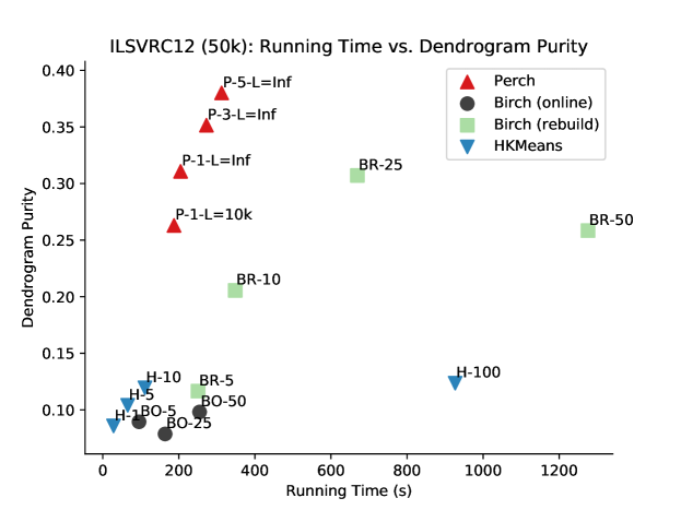
Figure 4: Speed vs. dendrogram purity on the ILSVRC12 50k dataset. Perch (P) is always more accurate than BIRCH (B) even when tuned so the running times are comparable. HKmeans (H) is also depicted for comparison against a fast, batch, tree building algorithm.

In Figure 4, we plot the dendrogram purity as a function of running time for the algorithms as we vary the relevant parameter. We use the ILSVRC12 (50K) dataset and run all algorithms on the same machine (28 cores with 2.40GHz processor).

The results show that Perch-BC achieves a better tradeoff between dendrogram purity and running time than the other methods. Except for in the uninteresting low purity regime, our algorithm achieves the best dendrogram purity for a given running time. HKMeans with few iterations can be faster, but it produces poor clusterings, and with more iterations the running time scales quite poorly. BIRCH with rebuilding performs well, but Perch-BC performs better in less time.

Our experiments also reveal that MB-KM is quite effective, both in terms of accuracy and speed. MB-KM is the fastest algorithm when the number of clusters is small while Perch is fastest when the number of clusters is very large. When the number of clusters is fairly small, MB-KM achieves the best speed-accuracy tradeoff. However, since the gradient computation in MB-KM are $O(K)$, the algorithm scales poorly when the number of clusters is large, while our algorithm, provided short trees are produced, has no dependence on $K$. For example, for ImageNet (100K) (the dataset with the largest number of clusters), MB-KM runs in $\sim$8007.93s (averaged over 5 runs) while Perch runs nearly twice as fast in 4364.37s. Faster still (although slightly less accurate) is Perch-BC which clusters the dataset in only 690.16s.

In Figure 5, we confirm empirically that insertion times scale with the size of the dataset. In the figure, we plot the insertion time and the maximum tree depth as a function of the number of data points on ILSVRC12 (50K). We also plot the same statistics for a variant of Perch that does not invoke balance-rotations to understand how tree structure affects performance.

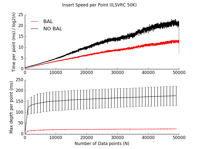
Figure 5: Insert speed divided by $\log_{2}(n)$ and max-depth as a function of the number of points inserted. Perch is the red (bottom) line and Perch without balance-rotations is black (top). Balancing helps to make insertion fast by keeping the tree short.

The top plot shows that Perch’s speed of insertion grows modestly with the number of points, even though the dimensionality of the data is high (which can make bounding box approximations worse). Both the top and bottom plots show that Perch’s balance rotations have a significant impact on its efficiency; in particular, the bottom plot suggests that the efficiency can be attributed to shallower trees. Recall that our analysis does not bound the depth of the tree or the running time of the nearest neighbor search. Thus in the worst case the algorithm may explore all leaves of the tree and have total running time scaling with $O(N^{2}d)$ where there are $N$ data points. Empirically we observe that this is not the case.

6.5 Robustness

We are also interested in understanding the performance of Perch and other online methods as a function of the arrival order. Perch is designed to be robust to adversarial arrival orders (at least under separability assumptions), and this section empirically validates this property. On the other hand, many online or streaming implementations of batch clustering algorithms can make severe irrecoverable mistakes on adversarial data sequences. Our (non-greedy) masking-rotations explicitly and deliberately alleviate such behavior.

To evaluate robustness, we run the algorithms on two adversarial orderings of the ALOI dataset:

• Sorted - the points are ordered by class (i.e., all $x\in C_{k}^{\star}\subset\mathcal{C}^{\star}$ are followed by all $x\in C_{i+1}^{\star}\subset\mathcal{C}^{\star}$, etc.)

• Round Robin - the $i^{th}$ point to arrive is a member of $C_{i\bmod K}^{\star}$ where $K$ is the true number of clusters.

The results in Tables 3(a) and 3(b) use a more benign random order.

Tables 3(d) and 3(c) contain the results of the robustness experiment. Perch performs best on round-robin. While Perch’s dendrogram purity decreases on the sorted order, the degradation is much less than the other methods. Online versions of agglomerative methods perform quite poorly on round-robin but much better on sorted orders. This is somewhat surprising, since the methods use a buffer size that is substantially larger than the number of clusters, so in both orders there is always a good merge to perform. For flat clusterings, we compare Perch with an online version of mini-batch K-means (o-MB-KM). This algorithm is restricted to pick clusters from the first mini-batch of points and not allowed to drop or restart centers. The o-MB-KM algorithm has significantly worse performance on the sorted order, since it cannot recover from separating multiple points from the same ground truth cluster. It is important to note the difference between this algorithm and the MB-KM algorithm used elsewhere in these experiments, which is robust to the input order. SKM++ improves since it uses a non-greedy method for the coreset construction. However, SKM++ is not technically an online algorithm, since it makes two passes over the dataset.

6.6 Small-scale Benchmarks

Finally, we evaluate our algorithm on the standard (small-scale) clustering benchmarks. While Perch is designed to be accurate and efficient for large datasets with many clusters, these results help us understand the price for scalability, and provide a more exhaustive experimental evaluation. The results appear in Table 6 and show that Perch is competitive with other batch and online algorithms (in terms of dendrogram purity), despite only examining each point once, and being optimized for large-scale problems.

	Glass	Digits	Spambase
Perch	0.474 $\pm$ 0.017	0.614 $\pm$ 0.033	0.611 $\pm$ 0.0131
BIRCH	0.429 $\pm$ 0.013	0.544 $\pm$ 0.054	0.595 $\pm$ 0.013
HKMeans	0.508 $\pm$ 0.008	0.586 $\pm$ 0.029	0.626 $\pm$ 0.000
HAC-C	0.47	0.594	0.628

Figure 6: Dendrogram purity on small-scale benchmarks.

7 Related Work

The literature on clustering is too vast for an in-depth treatment here, so we focus on the most related methods. These can be compartmentalized into hierarchical methods, online optimization of various clustering cost functions, and approaches based on coresets. We also briefly discuss related ideas in supervised learning and nearest neighbor search.

Standard hierarchical methods like single linkage are often the methods of choice for small datasets, but, with running times scaling quadratically with sample size, they do not scale to larger problems. As such, several online hierarchical clustering algorithms have been developed. A natural adaptation of these agglomerative methods is the mini-batch version that Perch outperforms in our empirical evaluation. BIRCH [39] and its extensions [20] comprise state of the art online hierarchical methods that, like Perch, incrementally insert points into a cluster tree data structure. However, unlike Perch, these methods parameterize internal nodes with means and variances as opposed to bounding boxes, and they do not implement rotations, which our empirical and theoretical results justify. On the other hand, Widyantoro et al. [38] instead use a bottom-up approach.

A more thriving line of work focuses on incremental optimization of clustering cost functions. A natural approach is to use stochastic gradient methods to optimize the K-means cost [10, 35]. Liberty et al. [26] design an alternative online K-means algorithm that when processing a point, opts to start a new cluster if the point is far from the current centers. This idea draws inspiration from the algorithm of Charikar et al. [12] for the online $k$-center problem, which also adjusts the current centers when a new point is far away. Closely related to these approaches are several online methods for inference in a probabilistic model for clustering, such as stochastic variational methods for Gaussian Mixture Models [24]. As our experiments demonstrate, this family of algorithms is quite effective when the number of clusters is small, but for problems with many clusters, these methods typically do not scale.

Lastly, a number of clustering methods use coresets, which are small but representative data subsets, for scalability. For example, the StreamKM++ algorithm of Ackermann et al. [2] and the BICO algorithm of Fichtenberger et al.  [20], run the K-means++ algorithm on a coreset extracted from a large data stream. Other methods with strong guarantees also exist [6], but typically coreset construction is expensive, and as above, these methods do not scale to the extreme clustering setting where $K$ is large.

While not explicitly targeting the clustering task, tree-based methods for nearest neighbor search and extreme multiclass classification inspired the architecture of Perch. In nearest neighbor search, the cover tree structure [8] represents points with a hierarchy while supporting online insertion and deletion, but it does not perform rotations or other adjustments that improve clustering performance. Tree-based methods for extreme classification can scale to a large number of classes, but a number of algorithmic improvements are possible with access to labeled data. For example, the recall tree [15] allows for a class to be associated with many leaves in the tree, which does not seem possible without supervision.

8 Conclusion

In this paper, we present a new algorithm, called Perch, for large-scale clustering. The algorithm constructs a cluster tree in an online fashion and uses rotations to correct mistakes and encourage a shallow tree. We prove that under a separability assumption, the algorithm is guaranteed to recover a ground truth clustering and we conduct an exhaustive empirical evaluation. Our experimental results demonstrate that Perch outperforms existing baselines, both in terms of clustering quality and speed. We believe these experiments convincingly demonstrate the utility of Perch.

Our implementation of Perch used in these experiments is available at: http://github.com/iesl/xcluster.

Acknowledgments

We thank Ackermann et. al [2] for providing us an implementation of StreamKM++ and BICO, and Luke Vilnis for many helpful discussions.

This work was supported in part by the Center for Intelligent Information Retrieval, in part by DARPA under agreement number FA8750-13-2-0020, in part by Amazon Alexa Science, in part by the National Science Foundation Graduate Research Fellowship under Grant No. NSF-1451512 and in part by the Amazon Web Services (AWS) Cloud Credits for Research program. The work reported here was performed in part using high performance computing equipment obtained under a grant from the Collaborative R&D Fund managed by the Massachusetts Technology Collaborative. Any opinions, findings and conclusions or recommendations expressed in this material are those of the authors and do not necessarily reflect those of the sponsor.

References

- [1]
- Ackermann et al. [2012] Marcel R Ackermann, Marcus Märtens, Christoph Raupach, Kamil Swierkot, Christiane Lammersen, and Christian Sohler. 2012. StreamKM++: A clustering algorithm for data streams. Journal of Experimental Algorithmics (JEA) (2012).
- Aggarwal et al. [2003] Charu C Aggarwal, Jiawei Han, Jianyong Wang, and Philip S Yu. 2003. A framework for clustering evolving data streams. In International Conference on Very Large Databases (VLDB).
- Ahmed et al. [2012] Amr Ahmed, Sujith Ravi, Alex J Smola, and Shravan M Narayanamurthy. 2012. Fastex: Hash clustering with exponential families. In Advances in Neural Information Processing Systems (NIPS).
- Arthur and Vassilvitskii [2007] David Arthur and Sergei Vassilvitskii. 2007. k-means++: The advantages of careful seeding. In Symposium on Discrete Algorithms (SODA).
- Bādoiu et al. [2002] Mihai Bādoiu, Sariel Har-Peled, and Piotr Indyk. 2002. Approximate clustering via core-sets. In Symposium on Theory of Computing (STOC).
- Betancourt et al. [2016] Brenda Betancourt, Giacomo Zanella, Jeffrey W Miller, Hanna Wallach, Abbas Zaidi, and Rebecca C Steorts. 2016. Flexible Models for Microclustering with Application to Entity Resolution. In Advances in Neural Information Processing Systems (NIPS).
- Beygelzimer et al. [2006] Alina Beygelzimer, Sham Kakade, and John Langford. 2006. Cover trees for nearest neighbor. In International Conference on Machine Learning (ICML).
- Blundell et al. [2011] Charles Blundell, Yee Whye Teh, and Katherine A Heller. 2011. Discovering non-binary hierarchical structures with Bayesian rose trees. Mixture Estimation and Applications (2011).
- Bottou and Bengio [1995] Léon Bottou and Yoshua Bengio. 1995. Convergence Properties of the K-Means Algorithms. In Advances in Neural Information Processing Systems (NIPS).
- Brown et al. [1992] Peter F Brown, Peter V Desouza, Robert L Mercer, Vincent J Della Pietra, and Jenifer C Lai. 1992. Class-based n-gram models of natural language. Computational linguistics (1992).
- Charikar et al. [1997] Moses Charikar, Chandra Chekuri, Tomás Feder, and Rajeev Motwani. 1997. Incremental clustering and dynamic information retrieval. In Symposium on Theory of Computing (STOC).
- Choromanska and Langford [2015] Anna E Choromanska and John Langford. 2015. Logarithmic time online multiclass prediction. In Advances in Neural Information Processing Systems (NIPS).
- Clauset et al. [2004] Aaron Clauset, Mark EJ Newman, and Cristopher Moore. 2004. Finding community structure in very large networks. Physical review E (2004).
- Daume III et al. [2016] Hal Daume III, Nikos Karampatziakis, John Langford, and Paul Mineiro. 2016. Logarithmic Time One-Against-Some. arXiv:1606.04988 (2016).
- Dehak et al. [2011] Najim Dehak, Patrick J Kenny, Réda Dehak, Pierre Dumouchel, and Pierre Ouellet. 2011. Front-end factor analysis for speaker verification. IEEE Transactions on Audio, Speech, and Language Processing (2011).
- Deng et al. [2009] Jia Deng, Wei Dong, Richard Socher, Li-Jia Li, Kai Li, and Li Fei-Fei. 2009. Imagenet: A large-scale hierarchical image database. In Computer Vision and Pattern Recognition (CVPR).
- Eisen et al. [1998] Michael B Eisen, Paul T Spellman, Patrick O Brown, and David Botstein. 1998. Cluster analysis and display of genome-wide expression patterns. Proceedings of the National Academy of Sciences (PNAS) (1998).
- Ester et al. [1996] Martin Ester, Hans-Peter Kriegel, Jörg Sander, Xiaowei Xu, and others. 1996. A density-based algorithm for discovering clusters in large spatial databases with noise.. In International Conference on Knowledge Discovery and Data Mining (KDD).
- Fichtenberger et al. [2013] Hendrik Fichtenberger, Marc Gillé, Melanie Schmidt, Chris Schwiegelshohn, and Christian Sohler. 2013. BICO: BIRCH meets coresets for k-means clustering. In European Symposium on Algorithms.
- Geusebroek et al. [2005] Jan-Mark Geusebroek, Gertjan J Burghouts, and Arnold WM Smeulders. 2005. The Amsterdam library of object images. International Journal of Computer Vision (IJCV) (2005).
- Gorban et al. [2008] Alexander N Gorban, Balázs Kégl, Donald C Wunsch, Andrei Y Zinovyev, and others. 2008. Principal manifolds for data visualization and dimension reduction. Springer.
- Heller and Ghahramani [2005] Katherine A Heller and Zoubin Ghahramani. 2005. Bayesian hierarchical clustering. In International Conference on Machine Learning (ICML).
- Hoffman et al. [2013] Matthew D Hoffman, David M Blei, Chong Wang, and John William Paisley. 2013. Stochastic variational inference. Journal of Machine Learning Research (JMLR) (2013).
- Krishnamurthy et al. [2012] Akshay Krishnamurthy, Sivaraman Balakrishnan, Min Xu, and Aarti Singh. 2012. Efficient active algorithms for hierarchical clustering. In International Conference on Machine Learning (ICML).
- Liberty et al. [2016] Edo Liberty, Ram Sriharsha, and Maxim Sviridenko. 2016. An algorithm for online k-means clustering. In Workshop on Algorithm Engineering and Experiments.
- Lichman [2013] M. Lichman. 2013. UCI Machine Learning Repository. (2013). http://archive.ics.uci.edu/ml
- Manning et al. [2008] Christopher D Manning, Prabhakar Raghavan, Hinrich Schütze, and others. 2008. Introduction to information retrieval. Vol. 1. Cambridge university press Cambridge.
- O’callaghan et al. [2002] Liadan O’callaghan, Nina Mishra, Adam Meyerson, Sudipto Guha, and Rajeev Motwani. 2002. Streaming-data algorithms for high-quality clustering. In International Conference on Data Engineering.
- Omohundro [1989] Stephen M Omohundro. 1989. Five balltree construction algorithms. International Computer Science Institute Berkeley.
- Ostrovsky et al. [2006] Rafail Ostrovsky, Yuval Rabani, Leonard J Schulman, and Chaitanya Swamy. 2006. The effectiveness of Lloyd-type methods for the k-means problem. In Foundations of Computer Science (FOCS).
- Pedregosa et al. [2011] F. Pedregosa, G. Varoquaux, A. Gramfort, V. Michel, B. Thirion, O. Grisel, M. Blondel, P. Prettenhofer, R. Weiss, V. Dubourg, J. Vanderplas, A. Passos, D. Cournapeau, M. Brucher, M. Perrot, and E. Duchesnay. 2011. Scikit-learn: Machine Learning in Python. Journal of Machine Learning Research 12 (2011), 2825–2830.
- Pruitt et al. [2012] Kim D Pruitt, Tatiana Tatusova, Garth R Brown, and Donna R Maglott. 2012. NCBI Reference Sequences (RefSeq): current status, new features and genome annotation policy. Nucleic acids research (2012).
- Russakovsky et al. [2015] Olga Russakovsky, Jia Deng, Hao Su, Jonathan Krause, Sanjeev Satheesh, Sean Ma, Zhiheng Huang, Andrej Karpathy, Aditya Khosla, Michael Bernstein, Alexander C. Berg, and Li Fei-Fei. 2015. ImageNet Large Scale Visual Recognition Challenge. International Journal of Computer Vision (IJCV) (2015).
- Sculley [2010] David Sculley. 2010. Web-scale k-means clustering. In International World Wide Web Conference (WWW).
- Sedgewick [1988] Robert Sedgewick. 1988. Algorithms. Pearson Education India.
- Szegedy et al. [2016] Christian Szegedy, Vincent Vanhoucke, Sergey Ioffe, Jon Shlens, and Zbigniew Wojna. 2016. Rethinking the inception architecture for computer vision. In Computer Vision and Pattern Recognition (CVPR).
- Widyantoro et al. [2002] Dwi H Widyantoro, Thomas R Ioerger, and John Yen. 2002. An incremental approach to building a cluster hierarchy. In International Conference on Data Mining (ICDM).
- Zhang et al. [1996] Tian Zhang, Raghu Ramakrishnan, and Miron Livny. 1996. BIRCH: an efficient data clustering method for very large databases. In ACM Sigmod Record.