Casimir EMF in configurations with shifted elements

Abstract

The possibility in principle is shown for the existence of Casimir electromotive force (EMF) in a configuration with parallel nanosized metal plates which are shifted relative one another. The effect is theoretically demonstrated for a configuration with two plates (wings) of finite length, the particular case of which is classical Casimir configuration with parallel plates. It is found that when the plates are strictly parallel, EMF does not appear. However, when the plates are shifted relative one another, in each of them time-constant EMF is generated. It is also found that maximal EMF values depending on the plate shifts are larger than those depending on the values of angles between the wings. All the found effects exist in periodic configurations with shifted elements. There are optima of the configuration geometrical parameters at which the EMF generation can be maximal.

INTRODUCTION

Recently the possibility in principle has been shown for the Casimir EMF existence in well-conducting nanosized individual Fateev:2015 and periodic Fateev:2016 configurations which are not closed in circuit. The effect is theoretically demonstrated with the use of configurations consisting of two nonparallel plates (wings). Naturally, in parallel metal plates in the classical configuration considered by Casimir Casimir:1948 ; Casimir:1949 , Milton:2001 ; Klimchitskaya:2009 ; Bordag:2009 no electromotive forces should appear. However, there can be fluctuations of electric potentials at the ends of the plates due to Johnson-Nyquist thermal noise Bimonte:2008 and interference currents because of radio interference.

The possibility of the Casimir EMF generation is associated with the effect which is similar to the light-induced electron drag which can appear in metals Gurevich:1992 , Shalaev:1992 ; Shalaev:1996 , graphite nano-films Mikheev:2012 ; Mikheev:2017 and semiconductors perovich:1981 . In our case, the drag effect can occur in nonparallel and well-conducting wings due to the resultant uncompensated action of virtual photons on electrons. Earlier it has been shown that in principle, in addition to the excitation of an EMF, the system with nonparallel wings can experience Casimir expulsion force Fateev:2012 and have some other interesting effects Fateev:2013 ; Fateev:2014 . The uncompensated action of forces on nonparallel configurations is due to the nonuniform action of Casimir forces on the opposite ends of the configuration asymmetrical along one of the coordinates. Both for the expulsion forces and for the EMF, the optimal parameters of the angles of nonparallel-plates opening and their lengths have been found at which the effects achieved should be maximal. In particular, when the plates in the configuration are shifted relative to one another, the forces of Casimir expulsion are not compensated as well Fateev:2014 . As the result, at some relative shifts, an increase in the expulsion forces of the entire configuration takes place, and torque moments and relaxation oscillation effects appear.

The question concerning the possibility and the properties of the EMF generation by nanosized metal configurations when their elements are shifted is quite interesting.

THEORY

Let us consider a configuration with nonparallel and shifted wings using it as an example for investigating the possibility of the existence of Casimir EMF. Let us note that each individual configuration presents by itself a figure comprised by flat metal plates (wings). The inner and outer surfaces of the figure should have the properties of almost perfect mirrors with the reflection coefficient $\rho$.

missing

Figure 1: ($c$) – the schematic view of a symmetrical configuration with a shifted left wing (length $R)$ by step $\Delta x$ against the $x$-axes direction, the particular case of which is parallel wings (for $\varphi=0)$ and a triangle (at $a=0$ and $\Delta x=0)$. The figure with the width $L$ in the $y$-axis direction (perpendicular to the plane of Figure $L$) is shown in the system of Cartesian coordinates $(x,z)$ Blue straight lines designate the virtual rays with the length $b$outgoing from the point $\mbox{M}_{1}$ at the limit angles $\Theta_{1}$ and $\Theta_{2}$ toward the figure right surface and finishing at the ends of the opposite wing of the figure at the points $\mbox{M}_{2}$ and $\mbox{M}_{3}$, respectively; ($d)$ – the schematic view of the rays passage at the limit angles $\Theta_{1}$and $\Theta_{2}$ from an arbitrary point $\mbox{M}_{1}$ of the left wing towards the ends of the right wing.

missing

Figure 2: Local intensities of the electric field $E$ generated along the parallel wings ($\varphi=0)$ at four different values of the relative shift $\Delta x/R$ for the same value of the distance $a$.

Let us present an individual configuration in the system of Cartesian coordinates in the form of two thin metal plates with the width $L$ (oriented along the $z$-axis) and surface length $R$ (a wing) located at the distance $a$ from one another; the opening angle $\varphi$ between the plates can be varied (by the same value for both wings simultaneously) as shown in Fig.1. Also let us take into consideration the possibility of the shift of one of the figure wings by the step $\Delta x$ in the direction opposite to the $x$-axis. For such geometry, the angle $\varphi$ should not be larger than the value $\varphi\leq\mbox{arccot}\left({{\Delta x}\mathord{\left/{\vphantom{{\Delta x}a}}\right.\kern-1.2pt}a}\right)$, otherwise the situation arises when the configuration of plates with two neighboring figures appears. This situation requires a different problem statement.

Further, let us note that for the above figures the concept developed in Ref. Fateev:2015 is completely applicable. The EMF for one wing of the figure $\Delta E_{\parallel}$ can be found in the first approximation in the following form Fateev:2015

$$\Delta E_{\parallel}=\frac{1}{2n_{b}e}\left[{1-\rho-k}\right]\int_{0}^{L}{dy}\int_{0}^{r_{\max}}{P(\Theta,r,\varphi)dr}$$ (1)

Here, $n_{b}$ - volume density, $e$ - electron charge, $\rho$- coefficient of reflection, $k$ - photon-transmission factor, $P(\Theta,r,\varphi)$ - local specific pressure at each point $\rho$ on the wing of the figure with the length $r_{\max}$ and width $L$

$$P(\Theta,r,\varphi)=\frac{\hbar c\pi^{2}}{240s^{4}}\int_{\Theta_{1}}^{\Theta_{2}}{d\Theta}\sin(\Theta-2\varphi)^{4}\sin\Theta\cos\Theta\\ =-\frac{\hbar c\pi^{2}}{240s^{4}}A(\varphi,\Theta_{1},\Theta_{2}),\\$$ (2)

where

$$\begin{array}[]{r}A(\varphi,\Theta_{1},\Theta_{2})=\frac{1}{96}\left[{24\Theta_{1}\sin 4\varphi-24\Theta_{2}\sin 4\varphi}\right.\\ +18\cos 2\Theta_{1}-18\cos 2\Theta_{2}\\ +6\cos(4\varphi-4\Theta_{2})-6\cos(4\varphi-4\Theta_{1})\\ +3\cos(8\varphi-2\Theta_{2})-3\cos(8\varphi-2\Theta_{1})\\ \left.{+\cos(8\varphi-6\Theta_{1})-\cos(8\varphi-6\Theta_{2})}\right].\\ \end{array}$$ (3)

In formula (2), $\hbar=h/2\pi$ - reduced Planck constant, and $c$- light speed; the functional expressions for the figure limit angles $\Theta_{{}_{1}}^{\mbox{right}},\;\Theta_{{}_{2}}^{\mbox{right}}$ for the right wing in the configuration taking into account relative shifts $\Delta x$ have the following form [16]

$$\Theta_{1}^{\mbox{right}}=\mbox{arcos}\left\{{-\frac{r+a\sin\varphi+\Delta x\cos\varphi-R\cos 2\varphi}{\sqrt{\left[{a+(R+r)\sin\varphi}\right]^{2}+\left[{\Delta x+(r-R)\cos\varphi}\right]^{2}}}}\right\},$$ (4)

$$\Theta_{{}_{2}}^{\mbox{right}}=\mbox{arccos}\left\{{-\frac{r+a\sin\varphi+\Delta x\cos\varphi}{\sqrt{a^{2}+\Delta x^{2}+r^{2}+2a\,r\sin\varphi+2\Delta x{\kern 1.0pt}r\cos\varphi}}}\right\}.$$ (5)

The limit angles $\Theta_{{}_{1}}^{\mbox{left}},\Theta_{2}^{\mbox{left}}$ for the left wing are found in the form

$$\Theta_{1}^{\mbox{left}}=\pi-\mbox{arcos}\left\{{-\frac{R+r+a\sin\varphi-\Delta x\cos\varphi-2R\cos^{2}\varphi}{\sqrt{\left[{a+(R+r)\sin\varphi}\right]^{2}+\left[{\Delta x+(R-r)\cos\varphi}\right]^{2}}}}\right\},$$ (6)

,

$$\Theta_{{}_{2}}^{\mbox{left}}=\mbox{arccos}\left\{{-\frac{r+a\sin\varphi-\Delta x\cos\varphi}{\sqrt{a^{2}+\Delta x^{2}+r^{2}+2a\,r\sin\varphi-2\Delta xr\cos\varphi}}}\right\}.$$ (7)

missing

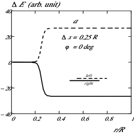
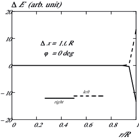
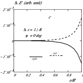
Figure 3: Integral values of the EMF $\Delta E$ generated along the parallel wings of the figure ($\varphi=0)$ at three different values of the relative shift $\Delta x/R$ for the same value of the distance $a$.

missing

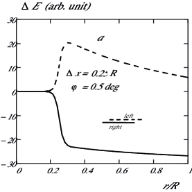
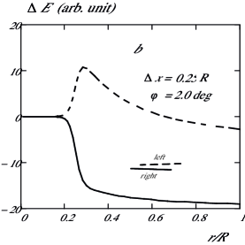
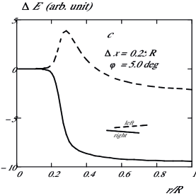
Figure 4: Integral values of the EMF $\Delta E$ generated along the figure nonparallel wings ($\varphi\neq 0)$ at three different values of the relative shift $\Delta x/R$ for the same value of the distance $a$.

In this case, the parameter $s$ in formula (2) will correspond to the right and left wings in the form

$$s^{\mbox{right}}=\frac{\sin(2\varphi-\Theta_{{}_{2}}^{\mbox{right}})(a+r\sin\varphi)}{\sin(\varphi-\Theta_{{}_{2}}^{\mbox{right}})},$$

$$s^{\mbox{left}}=\frac{\sin(2\varphi-\Theta_{{}_{2}}^{\mbox{left}})(a+r\sin\varphi)}{\sin(\varphi-\Theta_{{}_{2}}^{\mbox{left}})}.$$ (8)

Thus, here the basic diagram is presented for calculating the EMF generation in optical approximation in nanosized metal configurations due to virtual photons for the elements shifted relative to one another.

CALCULATION RESULTS

Using formulae (1-7), it is possible to find the following character of the EMF generation at the relative shift of two parallel plates which are not closed in circuit $\varphi=0$ and have the same length $R$; the distance between them is $a$ (see Fig.2). Integral electromotive forces corresponding to the shifts and generated along the entire length of each of the wings are shown in Fig.3. From Fig.2a it can be seen that without a shift ($\Delta x=0$), at the ends of both wings (the left wing - at $r/R=0$ and the right - at $r/R=1$) there are gradients of the electric-field $E$ potential absolutely similar in shape and value but oppositely directed. Consequently, in such system no EMF should generate. However, at the slightest relative shift ($\Delta x>0$) of the wings, the value and shape of the field $E$ intensity function nearby the ends have an asymmetrical character (Fig.2b). As the result, inside each of the wings, the EMF with an opposite relative gradient of the potentials should be generated (Fig.3a,b,c). In principle, the asymmetry of electric potentials should appear at any relative shift ($0<\Delta x<\infty$) changing only in shape and value (Fig.2c,d) but not in the direction of the gradient of the potentials for each of the two wings. Correspondingly, the EMF in the plates should be generated at any shift (Fig.3a,b,c). The same character of the dependences will be present at the rescaling of the dimensional parameters of the configuration to any small values within physically reasonable limits restricted by possible sizes of atoms and interatomic distances in the material of the metals plates.

The character of the EMF generation at the relative shift of two nonparallel plates ($\varphi\neq 0)$ significantly differs from that in the situation with parallel wings ($\varphi=0)$. For the wings with the same length $R$ and the minimal distance $a$ between them at the shift $\Delta x/R=0.25$, the following EMF behavior can be observed (Fig.4). It can be seen that for the same value of the shift, at the increase of the angle $\varphi$ and the growth of the left wing length $R$, the EMF generation decreases in the wing and the direction of the potential gradient changes to the opposite. At the same time, the EMF generation in the right wing only increases relative to that in the left one; though it decreases in the absolute value, but the potential gradient direction does not change.

missing

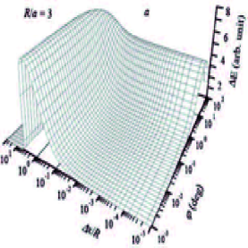
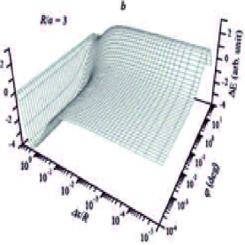
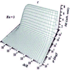
Figure 5: Joint EMF dependences on the shifts $\Delta x/R$ and angles $\varphi$ at $R/a=3$ for the left ($a)$ and the right ($b)$ wing with the total EMF (c) when they are connected in series in circuit.

missing

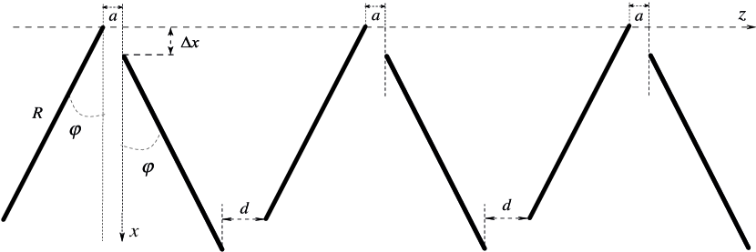
Figure 6: A schematic view of the periodic configuration with nonparallel figures located along the $z$-axis at the distance $d$ between them with the shift $\Delta x$.

The level of the EMF generation in the joint dependence on the shifts ($0\leq\Delta x/R\leq 40)$ and angles $0<\varphi\leq 90^{\circ}$ between the plates is shown in Fig.5a,b,c. In Fig.5 it is possible to observe interesting phenomena both for the left and for right wing. Firstly, similar to Figs.2 and 3, it can be seen that the EMF can be generated only at the shift of the plates relative to one another. Secondly, it appears that for both wings the maximal values (in the absolute value) of the EMF generation $\Delta E(\Delta x)$ depending on the shifts are larger, than the EMF maxima $\Delta E(\varphi)$ depending on the angles between the wings. At the shift, the maximum of the EMF generation remains at the same level at any angle $0<\varphi\leq 90^{\circ}$ (Fig.5a,b).

Let us note that when the two wings are connected in series in circuit, due to the shift the total EMF generation in them is completely compensated at any of the angle $0<\varphi\leq 90^{\circ}$ (Fig.5c). In this case, the shift $\Delta x/R>1$ leads to the gradual disappearance of the generation of the total EMF in the circuit due to the opening of the wings at any angle.

PERIODIC CONFIGURATIONS WITH SHIFTED ELEMENTS

Further, let us consider the character of the EMF generation in the chains of the wings shifted in relation to one another and placed in periodic configurations. Let it be the case of nonparallel figures periodically placed along the $z$-axis as shown in Fig.6. Each of the figures in the configuration period is completely similar to the individual figure (see Fig.1). In the period, between the ends of the figures there is a distance $d$. One on the wings is shifted along the $x$-axis by an arbitrary value $\Delta x$ in the direction of $x$-axis (one of the wing’s ends touches the $x$-axis) without a change in the angle $\varphi$

missing

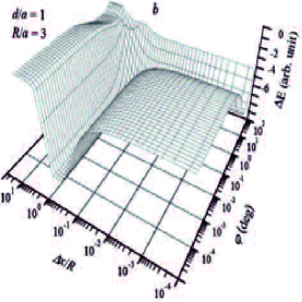
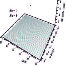
Figure 7: Joint dependences of the EMF on the shifts $\Delta x/R$ and angles $\varphi$ at $R/a=3$ for two electromotive forces in the right wing: ($a$) – when the gradient of the electric potential is increasing along the $x$-axis; ($b$) – when the gradient along the $x$-axis is decreasing; ($c$) – the sum of the two electromotive forces.

missing

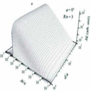
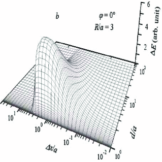
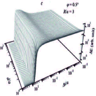
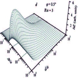
Figure 8: The EMF (a) and effectiveness $Q$ (b) dependences on the relations $d/a$ and shifts $\Delta x/a$ at $\varphi=0^{\circ}$ and $R/a=3$ in the periodic configuration, when the wings are connected in series in circuit; ($c$) and ($d$) similar dependences at $\varphi=0.5^{\circ}$.

missing

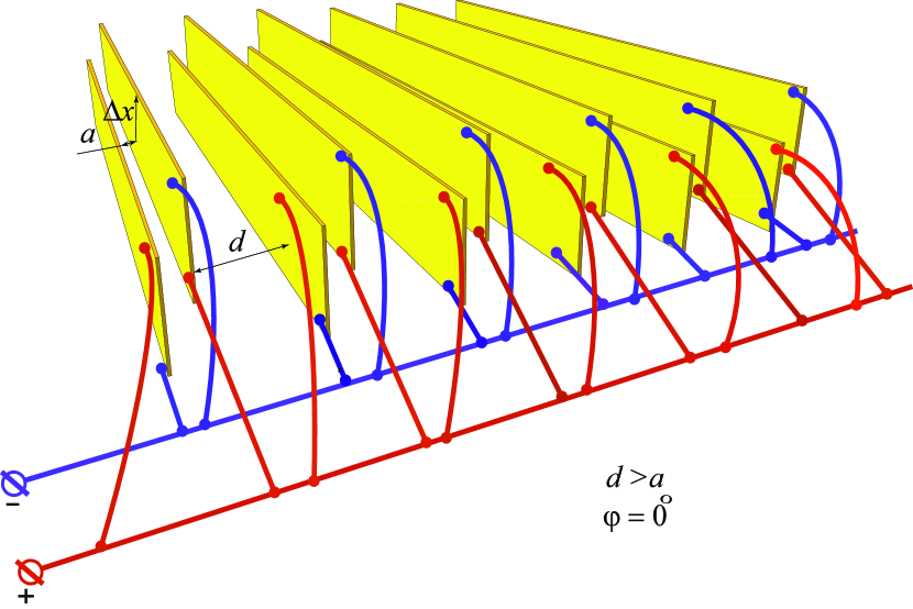
Figure 9: The plot of the Casimir EMF generator in the periodic configuration at the parallel connection of the wings in the circuit at the ratio $d/a>1$ and shift $\Delta x$ at $\varphi=0^{\circ}$

Similar to the paper on Casimir expulsion forces for periodic configurations with nonparallel figures [15], let us note the following. The periodic location of $n$ nonparallel figures, the wider opening of which is directed against the $x$-axis, with the distance $d$ between them leads to the formation of $n-1$ figures with oppositely directed openings (see Fig.2). In this case, a wing (one of the surfaces of a nonparallel figure) of each of the figures is a wing of another figure, the opening of which is directed to the opposite side. Thus, it is possible to write an expression for the total EMF for $n$ figures periodically located along the $z$-axis Rizzoni:2008 (when the wings are connected in series in circuit and not in parallel as sources of an EMF).

$$\Delta E_{\sum}=\sum\limits_{n=1}^{n}{\Delta E_{n}}=n\Delta E(a)-\left({n-1}\right)\Delta E(d).$$ (9)

Here, $\Delta E(a)$ is an EMF for the distance $a$ between the nearest ends of the figures and $\Delta E(d)$ is an EMF for the distance $d$, respectively, instead of $a$ in formulae (1-7). Naturally, when all the wings in the periodic configuration with nonparallel figures are connected in parallel and not in series in the electric circuit, it is more reasonable to calculate the sum of the equivalent summed current in the system.

CALCULATION RESULTS FOR PERIODIC CONFIGURATIONS WITH SHIFTED ELEMENTS

From formula (9) it follows that in the periodic configurations, for $d=a$ at any number $n$ of figures connected in series in circuit, Casimir EMF is $\Delta E_{\sum}\to\Delta E(a)$. That is, even for $n\to\infty$ at $d=a$ the EMF in the periodic configuration is always at the level of the EMF for one separate figure. It will happen due to the generation of two electromotive forces with opposite and equal gradients of the electric potential in each non-extreme wing in the periodic configuration as shown in Fig.7.

In accordance with formula (9), at $d\neq a$, the EMF of the periodic configuration will depend on the relation $d/a$. At the growth of $d/a$, the generation of EMF will tend to the dependence on shifts and angles, completely similar to that shown in Fig.7a. The electromotive forces in dependence on the growth of $d/a$ and shifts $\Delta x/a$ at certain angles and relations $R/a$ are shown in Fig.8a,c. At the growth of the number $n$ of nonparallel figures in the periodic configuration, the character of the curves will be similar to that of the curves presented; however, their total EMF will grow linearly at the growth of $n$ for any angles $\varphi$.

It is possible to determine the effectiveness $Q$ of the EMF generation for $n$ cavities with shifted elements as the relation of $\Delta E_{\sum}$ to the entire length of the configuration along the $z$-axis in the following form

$$Q=\frac{\Delta E_{\sum}}{n\left[{a+d+2R\tan(\varphi)}\right]}.$$ (10)

The dependence of $Q$ on the relations $d/a$ and shifts $\Delta x/a$ is shown in Fig.8b,d.

From Fig.8a, it can be seen that at any relations $d/a>1$, even for $\varphi=0^{\circ}$, at the relative shift of the wings $\Delta x/a$ in the circuit with in-series connection, an EMF can generate (see Fig.9). The EMF generation sharply decreases at $\Delta x/R>3$. For any length of the wings of the figure $R$ with different angles $\varphi$ there is a maximum of the effectiveness $Q$ of the generation of the total EMF $\Delta E_{\sum}$. At the EMF calculation in the configuration under study, for selected parameters, at $\varphi=0^{\circ}$, the optima of the relations $\Delta x/a\approx 1.5$ and $d/a\approx 1.8$ are found. In this case, for $R\to\infty$, the joint maximum exists at $\Delta x/a\to 2$ and $d/a\approx 1.8$. For nonparallel wings, for example, at the angle $\varphi=0.5^{\circ}$ the character of the dependences of the EMF and $Q$ changes significantly. In this case, the EMF generation is almost at the same level at any shifts (Fig.8c) starting with the smallest $\Delta x/R$. However, when the shifts are of the order $\Delta x/R>3$, at the angles $\varphi=0.5^{\circ}$ and $\varphi=0^{\circ}$ the EMF generation sharply decreases. The effectiveness is also higher at the angle $\varphi=0.5^{\circ}$ for the smaller relations $d/a$ and $\Delta x/a$ (Fig. 8d).

CONCLUSIONS

Thus, in the present paper, the possibility in principle is shown for the existence of Casimir EMF in nanosized parallel metal plates (wings) even at the smallest shift of one of them. It is found that the maximal values of the EMF generation depending on the shifts of the wings are even larger than the EMF maxima depending on the angles between the wings. The direction of the gradients of the electric-field potential in two shifted plates is opposite; however, it can change when the opening angle between them grows. It is found that the EMF generation is also possible in periodic configurations with shifted elements. The EMF generation takes place even in parallel configuration elements shifted with periodicity. There are optimal relations in the geometry of a shift and distances between the plates of the figures at which there can be a maximal EMF generation in the periodic configuration.

- (1) E.G. Fateev, Casimir EMF, arXiv:1502.03058 [physics.gen-ph], pp. 1-4, (2015).
- (2) E.G. Fateev, Casimir EMF in periodic configurations, arXiv:1601.07366 [physics.gen-ph], pp. 1-4, (2016).
- (3) H. B. G. Casimir, Kon. Ned. Akad. Wetensch. Proc. 51, 793 (1948).
- (4) H. B. G. Casimir and D. Polder, Phys. Rev. 73, 360–372 (1948).
- (5) K. A. Milton, The Casimir effect: Physical manifestations of zero-point energy, World Scientic, Singapore, 2001.
- (6) G. L. Klimchitskaya, U. Mohideen, V. M. Mostapanenko, Rev. Mod. Phys. 81, 1827–1885 (2009).
- (7) M. Bordag, G. L. Klimchitskaya, U. Mohideen, and V.M. Mostepanenko, Advances in the Casimir effect, Oxford University Press, Oxford, 2009.
- (8) G. Bimonte, J. Phys. A 41, 164013 (2008).
- (9) V. L. Gurevich, R. Laiho, and A. V. Lashkul, Phys. Rev. Lett. 69, 180–183 (1992).
- (10) V.M. Shalaev, C. Douketis, M. Moskovits, Physics Letters A 169, 205-210 (1992).
- (11) V. M. Shalaev, C. Douketis, J. Todd Stuckless, and M. Moskovits, Phys. Rev. B 53, N17 (1996).
- (12) G. M. Mikheev, A. G. Nasibulin, R.G. Zonov, A. Kaskela, and E. I. Kauppinen, Nano Lett. 12, 77?83 (2012).
- (13) G. M. Mikheev, A. S. Saushin, V. V. Vanyukov, K. G. Mikheev, Y. P. Svirko, Nanoscale Res. Lett, 12, 39 (2017).
- (14) V. L. Al’perovich, V. I. Belinicher, V. N. Novikov, A. S. Terekhov, JETP Lett, 33, N 11, 5 (1981).
- (15) E. G. Fateev, Casimir force of expulsion. : arXiv:1208.0303 [quant-ph], pp. 1-4,(2012).
- (16) E. G. Fateev, Casimir expulsion of periodic configurations: arXiv:1208.1256v1 [quant-ph], pp. 1-4,(2012).
- (17) E. G. Fateev, Casimir expulsion of shifted configurations. : arXiv:1301.1110 [quant-ph], pp. 1-8, (2013).
- (18) G. Rizzoni, Fundamentals of Electrical Engineering, McGraw-Hill Science, 2008, 736 p