Factorization, SUSY Coherent States and Classical Trajectories

^∗Musongela  Lubo ,^∗Kikunga  Kasenda Ivan ,^†Likwolo  Katamba Stanislas

^∗Physics Department, Faculty of Sciences, University of Kinshasa,P.O.Box Kin 190,Kinshasa, D.R.Congo
^†Faculty of Agronomy,University of Uele,P.O.Box Isiro 670, Isiro, D.R.Congo

Email : musongela.lubo@unikin.ac.cd, ivan.kikunga@unikin.ac.cd, likwolostanislas@yahoo.fr

Abstract

A generalization of coherent states has been developed in the context of supersymmetric quantum mechanics. For many cases, no link has been made with the corresponding classical system. In this work, we consider a very simple superpotential and compare the classical and quantum trajectories.

Keywords: Coherent States, SUSYQM.

1 Introduction

Coherent states and their applications in theoretical and technological fields have been the subject of many studies [1], [2], [3], [4], [5], [6], [7], [8], [9], [10], [11], [12], [13], [14], [15], [16], [17], [18] , [19] and [20].
Coherent states play an important role in quantum physics. Among their important properties is the fact that the mean value of the position operator in these states perfectly reproduce the classical behavior in the case of the harmonic oscillator. These states also saturate the Heisenberg inequality. Many generalizations have been proposed for the notion of coherent states for systems which are more complex than the harmonic oscillator. The path taken by supersymmetric quantum mechanics is a very simple one. When a Hamiltonian can be written as a product of an operator and its adjoint (plus a constant), one is basically in the situation of the harmonic oscillator with a creation and a destruction operator. The coherent states in this context are defined as the eigenvectors of the destruction operator. It has been shown that these states saturate a generalized uncertainty relation which is not the Heisenberg one [1].

For some potentials which play an important role in Physics and Chemistry (For example the Morse potential), the SUSY coherent states have been computed using a clever trick which bypasses the resolution of the Riccati equation for the determination of the superpotential [1]. But when it comes to the study of the mean value of the position or the momentum operator, one is confronted by the fact that these coherent states are not normalizable. One may try an approach using wave packets but the analysis becomes cumbersome.

The path taken here is the following. For the harmonic oscillator, the coherent states are normalizable. The superpotential is a one degree polynomial. To get an insight into the subject, we study an ad hoc system whose superpotential is polynomial. For simplicity and to ensure normalizability, we take it to be of third degree. The physical potential is then a sixth degree polynomial whose classical trajectories can be computed. The coherent states can be obtained in closed form. We than proceed to the calculation of the mean value of the position operator for these states. Comparison is then made with the classical trajectories.

The paper is organized as follows. The second section is a quick reminder of the formalism of SUSY coherent states that we need. The third section deals with the calculation of the mean value of the position operator in general. We apply it to a simple toy model in the fourth section. The treatment of the harmonic oscillator is put in the Appendix and shows that the analysis captures what is known by other methods.

2 A Quick Reminder of Coherent States and SUSYQM

There are many definitions of coherent states which are not exactly equivalent.

Let us first consider the case of the harmonic oscillator [26]. One has the following properties :

• The map $\mathbb{C}\owns z\longrightarrow\lvert z\rangle\in L^{2}(\mathbb{R})$ is continuous.

• $\lvert z\rangle$ is an eigenvector of the annihilation operator : $a\lvert z\rangle=z\lvert z\rangle$.

• The coherent states family resolves the unity $\frac{1}{\pi}\ \int_{\mathbb{C}}\lvert z\rangle\langle z\rvert d^{2}z=\mathbf{1}$.

• The coherent states saturate the Heisenberg inequality : $\Delta q\ \Delta p=\frac{1}{2}$.

• The coherent states family is temporally stable.

• The mean value (or ” lower symbol ”) of the Hamiltonian mimics the classical energy-action relation : $\check{H}(z)=\langle z\lvert\mathbf{\hat{H}}\rvert z\rangle=\omega\lvert z\rvert^{2}+\frac{1}{2}$.

• The coherent states family is the orbit of the ground state under the action of the Weyl-Heisenberg displacement operator : $\lvert z\rangle=e^{(za^{\dagger}-\overline{z}z)}\lvert 0\rangle\equiv D(z)\lvert 0\rangle$.

• The coherent states provide a straightforward quantization scheme : Classical state $z\longrightarrow\lvert z\rangle\langle z\rvert$ Quantum state.

• The mean value of the position operator in these states reproduce the classical trajectories.

One studies a system which admits an infinite set of discrete energies obeying the ”partition” of unity.

Let us consider a system with an infinite set of eigen energies which resolves unity.

$$\begin{split}\hat{H}\lvert\psi_{n}\rangle&=E_{n}\lvert\psi_{n}\rangle,\\ \langle\psi_{m}\lvert\psi_{n}\rangle&=\delta_{m,n},\\ \sum_{m=1}^{+\infty}\lvert\psi_{m}\rangle\langle\psi_{m}\rvert&=1.\end{split}$$ (1)

One introduces the raising and lowering operators by the relations

$$\begin{split}A^{-}\lvert\psi_{n}\rangle&=\sqrt{k(n)}\lvert\psi_{n-1}\rangle,\\ A^{+}\lvert\psi_{n}\rangle&=\sqrt{k(n+1)}\lvert\psi_{n+1}\rangle,\\ \rho(n)&=\prod_{i=1}^{n}k(i),\ \rho(0)=1.\end{split}$$ (2)

For the harmonic oscillator $k(i)=i$.
The coherent states can be defined as the eigenvectors of the lowering operator [30].

$$A^{-}\lvert z,\alpha\rangle=z\lvert z,\alpha\rangle.$$ (3)

It is possible to show that the time evolution sends a coherent state to another coherent state, with different parameters.
All coherent states can be obtained by acting on the ground state by the displacement operator.
The definition adopted by Klauder [16] is that the coherent states are given by

$$\lvert\psi(z)\rangle=\frac{1}{\sqrt{{\cal{N}}(\lvert z\rvert^{2})}}\sum_{n\in I}\frac{z^{n}}{\sqrt{\rho(n)}}\lvert\psi_{n}\rangle,$$ (4)

where $\cal{N}$ is the normalization factor.

The general squeezed coherent states for a quantum system with an infinite discrete energy spectrum was defined in [23] by the relation

$$(A^{-}+\gamma A^{+})\psi(z,\gamma)=z\psi(z,\gamma),$$ (5)

with $z,\gamma\in\mathbb{C}$.
For a system whose discrete spectrum is finite (Example : The Morse potential) another generalization was studied [23].
It ressembles (4) but now the sum runs on a finite number of indices.

Let us now turn to SUSYQM. Consider a system described by a potential $V_{0}$ which admits a ground state energy satisfying the Schroedinger equation

$$-\frac{1}{2}u^{(0)^{\prime\prime}}+V_{0}u^{(0)}=\varepsilon u^{(0)}.$$ (6)

Introduce the function

$$\alpha_{1}=\frac{u^{(0)^{\prime}}}{u^{(0)}}$$ (7)

and the new potential

$$V_{1}=V_{0}-\alpha_{1}.$$ (8)

Looking at the Hamiltonians

$$H_{0}=-\frac{1}{2}\frac{d^{2}}{dx^{2}}+V_{0}(x),\ H_{1}=-\frac{1}{2}\frac{d^{2}}{dx^{2}}+V_{1}(x),$$ (9)

one sees that they can be factorized in the following way

$$\begin{split}H_{0}&=A_{1}A_{1}^{+}+\varepsilon,\\ H_{1}&=A_{1}^{+}A_{1}+\varepsilon,\end{split}$$ (10)

where the operators involved are given by the formulas

$$A_{1}=\frac{1}{\sqrt{2}}\bigg{[}\frac{d}{dx}+\alpha_{1}(x)\bigg{]},\ A_{1}^{+}=\frac{1}{\sqrt{2}}\bigg{[}-\frac{d}{dx}+\alpha_{1}(x).\bigg{]}.$$ (11)

One has the intertwining relations

$$H_{1}A_{1}^{+}=A_{1}^{+}H_{0},\ H_{0}A_{1}=A_{1}H_{1},$$ (12)

from which one finds the spectrum of $H_{1}$ (knowing that of $H_{0}$) and the link between their eigenstates. So far for factorization and intertwining. The introduction of SUSYQM can then proceed as follows. One introduces the operators

$$Q=\begin{pmatrix}0&0\\ A_{1}&0\end{pmatrix},\ Q^{+}=\begin{pmatrix}0&A_{1}^{+}\\ 0&0\end{pmatrix},$$ (13)

and sees that the Hamiltonian takes the form

$$\begin{split}H_{SUSY}&=\big{\{}Q,Q^{+}\big{\}}\\ &=\begin{pmatrix}H_{1}-\varepsilon&0\\ 0&H_{0}-\varepsilon\end{pmatrix}.\end{split}$$ (14)

Introducing

$$\begin{split}Q_{1}=\frac{1}{\sqrt{2}}\left(Q^{+}+Q\right),\\ Q_{2}=\frac{1}{i\sqrt{2}}\left(Q^{+}-Q\right),\end{split}$$ (15)

one has

$$\begin{split}[Q_{i},H_{SUSY}]&=0,\\ \big{\{}Q^{+}_{i},Q_{j}\big{\}}&=\delta_{ij}H_{SUSY},\ i,j=1,2.\end{split}$$ (16)

3 Our Approach

We are studying a one dimensional system with a rescaled undimensional coordinate q. Suppose one can write the physical potential $V(q)$ of such a system in terms of a function $x(q)$ by the relation

$$V(q)-E_{0}=\frac{1}{2}\Big{[}x^{2}(q)+\frac{dx(q)}{dq}\Big{]}.$$ (17)

Then one can factorize the Hamiltonian

$$\hat{H}=\hat{A^{\dagger}}\hat{A}+E_{0},$$ (18)

where the operators $A$ and $\hat{A^{\dagger}}$ have the form

$$\hat{A}=\frac{1}{\sqrt{2}}\Big{[}\frac{d}{dq}-x(q)\Big{]};\ \hat{A^{\dagger}}=\frac{1}{\sqrt{2}}\Big{[}-\frac{d}{dq}-x(q)\Big{]};$$ (19)

so that

$$\Big{[}\hat{A},\hat{A^{\dagger}}\Big{]}=-\frac{dx(q)}{dq}.$$ (20)

The function $x(q)$ is called the superpotential. Eq.(19) and (20) are reminiscent of the harmonic oscillator. Using that similarity, the coherent states are defined as the eigenfunctions of the ”annihilation operator” $\hat{A}$. Using Eq.(19) one is led to an equation of separable variables. The solution reads

$$\psi_{H}(q,\alpha)=N\exp{\Big{[}\sqrt{2}\alpha q+\int_{0}^{q}x(\xi)\,d\xi\Big{]}}.$$ (21)

In Eq.(21), $\alpha$ is a complex variable which characterizes the coherent states. When trying to implement the SUSY treatment to a system whose physical potential is known, the difficult part is the resolution of the Riccati equation given in Eq.(17).
For the harmonic oscillator, one introduces the rescaled variables

$$Q=\sqrt{\frac{\hbar}{m\omega}}\ q\hskip 14.22636pt;\hskip 14.22636pt\ P=\sqrt{m\omega\hbar}\ p,$$ (22)

and the rescaled potential

$$U(Q)=\hbar\omega\ V(q).$$ (23)

The superpotential is given by

$$x(q)=-q,$$ (24)

so that the coherent state takes the form

$$\psi_{H}(q,\alpha)=N\exp{(\sqrt{2}\alpha q-\frac{1}{2}q^{2})},$$ (25)

which is normalizable.

For the Morse potential, the superpotential is given by [1]

$$x(q)=\frac{-s+\exp{(-q\hskip 2.84526pt\sqrt{2\chi_{e}}})}{\sqrt{2\chi_{e}}}+\sqrt{\frac{\chi_{e}}{2}},$$ (26)

the parameters $s$ and $\chi_{e}$ are related to the Morse potential’s energy levels:

$$E_{n}=s\left(n+\frac{1}{2}\right)-\chi_{e}\left(n+\frac{1}{2}\right)^{2}.$$ (27)

So, the coherent states takes the form

$$\psi_{H}(q,\alpha)=\exp{\Big{[}-\frac{1}{2\chi_{e}}\exp{(-q\hskip 2.84526pt\sqrt{2\chi_{e}})}-\frac{s-\chi_{e}}{\sqrt{2\chi_{e}}}q+\sqrt{2}\alpha q\Big{]}}.$$ (28)

Clearly, such a function in not square integrable and the mean values can not be computed.

The aim of this paper is to construct a superpotential such that the corresponding coherent states are normalizable and the computation of the mean values not too complicated. The quantity we are interested in is the mean value

$$\langle\hat{q}\rangle=\frac{\langle\psi_{S,t}\lvert\hat{q}\rvert\psi_{S,t}\rangle}{\langle\psi_{S,t}\lvert\psi_{S,t}\rangle}.$$ (29)

One has to realize that the states given in Eq.(21) were obtained in the Heisenberg picture : the wave function does not depend on time. To pass to the Schrodinger picture one has to use the evolution operator

$$\lvert\psi_{S,t}\rangle=\exp{(-\frac{i}{\hbar}\hat{\mathbf{H}}t)}\rvert\psi_{H}\rangle,$$ (30)

where the Hamiltonian takes the form

$$\hat{\mathbf{H}}=\hbar\omega\Big{[}\frac{\hat{p}^{2}}{2}+\hat{V}(q)\Big{]}.$$ (31)

The factorization of the Hamiltonian and the evolution operator can be used to obtain the wave function in the Schrodinger picture as a power series

$$\lvert\psi_{S,t}\rangle=\exp(-\frac{i}{\hbar}E_{0}t).\sum_{k=0}^{n}(-i)^{k}\frac{(\omega t)^{k}}{k!}(\hat{A^{+}}\hat{A})^{k}\lvert\psi_{H}\rangle.$$ (32)

The mean value then reads

$$\langle\psi_{S,t}\lvert\hat{q}\rvert\psi_{S,t}\rangle=\sum_{m=0}^{\infty}\sum_{n=0}^{\infty}\frac{(-1)^{m}i^{m+n}}{m!n!}t^{m+n}\langle\psi_{H}\lvert\hat{H}^{n}\hat{q}\hat{H}^{m}\rangle\psi_{H}\rangle.$$ (33)

The relation

$$\hat{A^{\dagger}}=-\hat{A}-\sqrt{2}x(q)$$ (34)

is obtained by adding the two relations given in Eq.(19).
With the fact that the wave function, we are studying, is an eigenvector of the ”annihilation operator”, we find

$$\hat{A^{\dagger}}\hat{A}\lvert\psi_{H}\rangle=\alpha\Big{[}-\alpha-\sqrt{2}x(q)\Big{]}\rvert\psi_{H}\rangle.$$ (35)

Subtracting the relations in (19), we similarly find

$$\frac{\partial}{\partial q}\lvert\psi_{H}\rangle=\Big{[}\sqrt{2}\alpha+x(q)\Big{]}\rvert\psi_{H}\rangle.$$ (36)

This allows us to obtain the second order contribution of the wave function

$$(\hat{A^{\dagger}}\hat{A})^{2}\lvert\psi_{H}\rangle=\Big{[}\alpha\frac{\sqrt{2}}{2}\frac{d^{2}x(q)}{dq^{2}}+\left(2\alpha^{2}+\sqrt{2}\alpha x(q)\right)\frac{dx(q)}{dq}+\left(\sqrt{2}\alpha x(q)+\alpha^{2}\right)^{2}\Big{]}\rvert\psi_{H}\rangle.$$ (37)

This suggests the introduction of special functions $f_{n}$ such that

$$(\hat{A^{\dagger}}\hat{A})^{n}\lvert\psi_{H}\rangle=f_{n}(q,\alpha)\psi_{H}\rangle.$$ (38)

From the previous considerations, one derives the recurrence formula

$$f_{n+1}=-\frac{1}{2}\frac{\partial^{2}f_{n}}{\partial q^{2}}-\Big{[}\sqrt{2}\alpha+x(q)\Big{]}\frac{\partial f_{n}}{\partial q}-\Big{[}\sqrt{2}\alpha x(q)+\alpha^{2}\Big{]}f_{n}.$$ (39)

Note that

$$f_{0}(q,\alpha)=1.$$ (40)

Working in the position representation, the time dependent wave function

$$\psi_{S}(q,t,\alpha)=\exp{(-\frac{i}{\hbar}E_{0}t)}\sum_{m=0}^{\infty}\frac{(-i\omega t)^{m}}{m!}\Big{[}(\hat{A^{\dagger}}\hat{A})^{m}\psi_{H}(q,\alpha)\Big{]}$$ (41)

takes the form

$$\psi_{S}(q,t,\alpha)=\exp{(-\frac{i}{\hbar}E_{0}t)}\sum_{m=0}^{\infty}\frac{(-i\omega t)^{m}}{m!}f_{m}(q,\alpha)\psi_{H}(q,\alpha).$$ (42)

The position mean value is then given by an infinite double sum

$$_{S}\langle\psi\lvert\hat{q}\rvert\psi\rangle_{S}=\sum_{m=0}^{\infty}\sum_{n=0}^{\infty}\frac{i^{m+n}(-1)^{n}}{m!n!}C_{m,n}\ (\omega t)^{m+n}$$ (43)

where the coefficients $C_{m,n}$ are the integrals

$$C_{m,n}=\int_{-\infty}^{+\infty}dq.qf^{*}_{m}(q,\alpha)f_{n}(q,\alpha)\psi_{H}^{*}(q,\alpha)\psi_{H}(q,\alpha)\ .$$ (44)

The double summation can be rewritten as a power series in the time parameter

$$_{S}\langle\psi\lvert\hat{q}\rvert\psi\rangle_{S}=\sum_{l=0}^{\infty}(\omega t)^{l}\Omega_{l},$$ (45)

with

$$\Omega_{l}=i^{l}(-1)^{l}\sum_{m=0}^{l}\frac{(-1)^{m}}{m!(l-m)!}C_{m,l-m}.$$ (46)

Explicitly, we can write

$$\begin{split}\Omega_{0}&=C_{0,0},\\ \Omega_{1}&=-i\left(C_{0,1}-C_{1,0}\right),\\ \Omega_{2}&=\frac{1}{2!}\left(-C_{0,2}+2C_{1,1}-C_{2,0}\right),\\ \Omega_{3}&=i[\ \frac{1}{2!}\left(C_{2,1}-C_{1,2}\right)+\frac{1}{3!}\left(C_{0,3}-C_{3,0}\right)\ ],\\ \Omega_{4}&=\frac{1}{4!}\left(C_{0,4}+C_{4,0}\right)-\frac{1}{3!}\left(C_{1,3}+C_{3,1}\right)+\frac{1}{2!\ 2!}\ C_{2,2},\\ &\cdots\end{split}$$ (47)

Eq.(45) is written with the fact the quantity ${}_{S}\langle\psi\lvert\psi\rangle_{S}$ is an unessential constant.
One can consider that Eq.(45) and Eq.(46) gives the answer to our question about the mean value of the position operator in this context. For any practical case, one has to compute the integrals of Eq.(44) and makes the appropriate summation.
At this point one has to point technical difficulties. The first one is that the recursion relations of Eq.(39) can quickly leads to large formulas even for simple superpotentials. The second one is that it is not always possible to have an analytical expression for the integrals appearing in Eq.(44). Third, one has to be careful about the order at which one can stop to in the series Eq.(45) to obtain a reliable estimate.

To test our approach, we first used it on the harmonic oscillator. The results are good and reproduce some important characteristics of the coherent states as known in the literature.

The solution to the classical equations of motion is given by

$$q_{class}(t)=C_{1}\cos{\omega t}+C_{2}\sin{\omega t},$$ (48)

where $C_{1}$ and $C_{2}$ are constants.
This can be written as a power series

$$q(t)=A_{0}+A_{1}\omega t+A_{2}(\omega t)^{2}+\cdots$$ (49)

where one has

$$\frac{A_{2}}{A_{0}}=-\frac{1}{2},\ \frac{A_{3}}{A_{1}}=-\frac{1}{6},\cdots$$ (50)

We can write the ”quantum trajectory” as

$$\langle\psi_{S,t}\lvert\hat{q}\rvert\psi_{S,t}\rangle=\sum_{l=0}^{+\infty}\Omega_{l}.(\omega t)^{l}.$$ (51)

It can be shown that the classical trajectory verifies the same relations i.e.

$$\frac{\Omega_{2}}{\Omega_{0}}=-\frac{1}{2},\ \frac{\Omega_{3}}{\Omega_{1}}=-\frac{1}{6},\cdots$$ (52)

To keep our presentation light, we have put this treatment in the Appendix.

4 A Toy Model

The generalization of coherent states considered here was introduced in [1]. For many potentials used in theoretical chemistry, the corresponding states are not normalizable and this leads to technical difficulties when one is interested in mean values. We want to restrict ourselves to systems with square integrable generalized coherent states. In the context of quantum supersymetry, the most important ingredient is the superpotential. For the harmonic oscillator, the superpotential in linear in the position. The next non trivial thing is to study a polynomial superpotential. A second degree superpotential is readily seen to lead to a non normalizable generalized coherent state. This leads us to study a toy model whose superpotential is given by

$$x(q)=x_{1}q-\frac{1}{3}x_{1}^{2}q^{3},$$ (53)

with

$$x_{1}<0,$$ (54)

where $x_{1}$ is a free parameter.
The corresponding physical potential is a sixth degree polynomial (See Eq.(17))

$$U(Q)=\hbar\omega(U_{0}+U_{2}Q^{2}+U_{4}Q^{4}+U_{6}Q^{6}).$$ (55)

Its coefficients are related to those of the rescaled superpotential by

$$U_{0}=0;\ U_{2}=0;\ U_{4}=-(\frac{\hbar}{m\omega})^{2}\frac{x_{1}^{3}}{3};\ U_{6}=(\frac{\hbar}{m\omega})^{3}\frac{x_{1}^{4}}{18}.$$ (56)

It has to be noted that if one begins with the potential, the characteristic frequency is given by

$$\hbar\omega=\frac{U^{3}_{4}}{U^{2}_{6}}.$$ (57)

This potential has the form given in Fig.1 given in the next page.

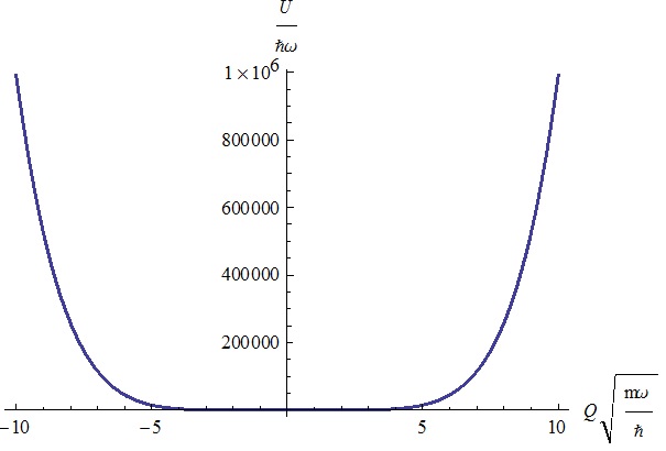
Figure 1: A Potential for the Toy Model for the values $U_{4}=1$ and $U_{6}=1$.

Classically, all the trajectories are bounded and periodic, with the period

$$T_{class}=4\sqrt{\frac{2}{m}}\int_{0}^{Q_{+}}\frac{1}{\sqrt{E-U(Q)}}dQ\$$ (58)

which depends on the energy of the system because $Q_{+}$ is such that $E-U(Q_{+})=0$.
We now analyze the mean value of the position operator for the corresponding coherent states and compare them with the classical trajectories. From Eq.(39) one easily sees that the functions $f_{n}$ will be polynomial in the the variable $q$. This will highly simplify the computations. We thus introduce the coefficients $\tilde{f}_{n}(\alpha)$ by

$$f_{n}(q,\alpha)=\sum_{k=0}^{3n}\tilde{f}_{n,k}(\alpha)q^{k}$$ (59)

with

$$\tilde{f}_{0,0}=\tilde{f}_{0,0}^{\star}=1.$$ (60)

The coefficients we have introduced obey the following recursion relations which naturally come from Eq.(39):

$$\begin{split}\tilde{f}_{n+1,0}&=-\tilde{f}_{n,2}-\sqrt{2}\alpha\tilde{f}_{n,1}-\alpha^{2}\tilde{f}_{n,0};\\ \tilde{f}_{n+1,1}&=-3\tilde{f}_{n,3}-2\sqrt{2}\alpha\tilde{f}_{n,2}-(x_{1}+\alpha^{2})\tilde{f}_{n,1}-\sqrt{2}\alpha x_{1}\tilde{f}_{n,0};\\ \tilde{f}_{n+1,2}&=-6\tilde{f}_{n,4}-3\sqrt{2}\alpha\tilde{f}_{n,3}-(2x_{1}+\alpha^{2})\tilde{f}_{n,2}-\sqrt{2}\alpha x_{1}\tilde{f}_{n,1};\\ \tilde{f}_{n+1,l}&=-\frac{1}{2}(l+1)(l+2)\tilde{f}_{n,l+2}-\sqrt{2}\alpha(l+1)\tilde{f}_{n,l+1}-(x_{1}l+\alpha^{2})\tilde{f}_{n,l}-\sqrt{2}\alpha x_{1}\tilde{f}_{n,l-1}\\ &+\frac{1}{3}x_{1}^{2}(l-2)\tilde{f}_{n,l-2}+\frac{\sqrt{2}}{3}\alpha x_{1}^{2}\tilde{f}_{n,l-3}\ (3<l<3n-2);\\ \tilde{f}_{n+1,3n-1}&=-3n\sqrt{2}\alpha\tilde{f}_{n,3n}-[(3n-1)x_{1}+\alpha^{2}]\tilde{f}_{n,3n-1}-\sqrt{2}\alpha x_{1}\tilde{f}_{n,3n-2}\\ &+\frac{1}{3}x_{1}^{2}(3n-3)\tilde{f}_{n,3n-3}+\frac{\sqrt{2}}{3}\alpha x_{1}^{2}\tilde{f}_{n,3n-4};\\ \tilde{f}_{n+1,3n}&=-(3nx_{1}+\alpha^{2})\tilde{f}_{n,3n}-\sqrt{2}\alpha x_{1}\tilde{f}_{n,3n-1}+\frac{1}{3}x_{1}^{2}(3n-2)\tilde{f}_{n,3n-2}+\frac{\sqrt{2}}{3}\alpha x_{1}^{2}\tilde{f}_{n,3n-3};\\ \tilde{f}_{n+1,3n+1}&=-\sqrt{2}\alpha x_{1}\tilde{f}_{n,3n}+\frac{1}{3}x_{1}^{2}(3n-1)\tilde{f}_{n,3n-2}+\frac{\sqrt{2}}{3}\alpha x_{1}^{2}\tilde{f}_{n,3n-2};\\ \tilde{f}_{n+1,3n+2}&=nx_{1}^{2}\tilde{f}_{n,3n}+\frac{\sqrt{2}}{3}\alpha x_{1}^{2}\tilde{f}_{n,3n-1};\\ \tilde{f}_{n+1,3n+3}&=\frac{\sqrt{2}}{3}\alpha x_{1}^{2}\tilde{f}_{n,3n}.\end{split}$$ (61)

We know have to compute

$$C_{m,n}=\sum_{k=0}^{m}\sum_{p=0}^{n}\int_{-\infty}^{+\infty}dq.q^{k+p+1}\tilde{f^{\star}}_{m,k}(\alpha)\tilde{f}_{n,p}(\alpha)\exp{(2\beta q+x_{1}q^{2}-\frac{1}{6}x_{1}^{2}q^{4})}\ .$$ (62)

From Eq.(62), we have

$$C_{0,0}=\int_{-\infty}^{+\infty}dq.q\ \exp{(2\beta q+x_{1}q^{2}-\frac{1}{6}x_{1}^{2}q^{4})}\ .$$ (63)

The integrals in Eq.(62) have the generic form

$$J_{n}=\int_{-\infty}^{+\infty}dq.q^{n}\ \exp{(2\beta q+x_{1}q^{2}-\frac{1}{6}x_{1}^{2}q^{4})}\ .$$ (64)

At this point, there are two ways to tackle the computation. The first insight is that one may need to compute only the integral $J_{0}$. The second one will use recursion relations.
We begin with the first approach. Its main interest relies in the fact that it leads to analytical expressions. Its main limitation is that it works only for big values of the real part of the parameter $\alpha$ describing th coherent state.

In short, from Eq.(64) it can be shown that

$$J_{n}=\frac{1}{2^{n}}\frac{d^{n}}{d\beta^{n}}J_{0}.$$ (65)

For convenience, we introduce the function

$$g(q)=2\beta q+x_{1}q^{2}-\frac{1}{6}x_{1}^{2}q^{4}.$$ (66)

Our integral then becomes

$$J_{0}=\int_{-\infty}^{\infty}dq\ \exp{[g(q)]}.$$ (67)

To evaluate $J_{0}$, we shall use the saddle point approximation. This is due to the fact that the exponential is a very rapidly decaying function, due to the fourth degree term with a negative sign in the exponential. The extrema of the integrand satisfy the equation

$$q^{3}-\frac{3}{x_{1}}q-\frac{3\beta}{x_{1}^{2}}=0.$$ (68)

This equation is a particular case of the following

$$q^{3}+a_{1}q^{2}+a_{2}q+a_{3}=0.$$ (69)

The solution to such an equation can be recast using the Cardan formula. One introduces the intermediate quantities

$$Q=\frac{-1}{x_{1}};R=\frac{3\beta}{2x_{1}^{2}};$$ (70)

$$D=Q^{3}+R^{2};S=\sqrt[3]{R+\sqrt{D}};\ T=\sqrt[3]{R-\sqrt{D}}.$$ (71)

The only real extremum (actually a maximum) is found at

$$q_{0}=S+T-\frac{1}{3}a_{1}.$$ (72)

One finally arrives at the following expression

$$q_{0}=\sqrt[3]{\frac{3\beta}{2x_{1}^{2}}+\sqrt{\frac{9\beta^{2}}{4x_{1}^{4}}-\frac{1}{x_{1}^{3}}}}+\sqrt[3]{\frac{3\beta}{2x_{1}^{2}}-\sqrt{\frac{9\beta^{2}}{4x_{1}^{4}}-\frac{1}{x_{1}^{3}}}}.$$ (73)

Let us first expand the function $g$, given by (66), near its minimum

$$g(q)=g(q_{0})+\frac{1}{2!}g^{\prime\prime}(q_{0})(q-q_{0})^{2}+\frac{1}{3!}g^{\prime\prime\prime}(q_{0})(q-q_{0})^{3}+\frac{1}{4!}g^{(4)}(q_{0})(q-q_{0})^{4}+\cdots$$ (74)

Introducing the centered and rescaled variable $y$ by

$$q=q_{0}+\frac{y}{\sqrt{-g^{\prime\prime}(q_{0})}}$$ (75)

one obtains

$$g(q)=g(q_{0})-\frac{1}{2!}y^{2}+Ay^{3}+By^{4}+\cdots$$ (76)

where the parameters $A$ and $B$ are given by

$$A=\frac{1}{3!}\ \frac{g^{(3)}(q_{0})}{[-g^{\prime\prime}(q_{0})]^{\frac{3}{2}}},\ B=\frac{1}{4!}\ \frac{g^{(4)}(q_{0})}{[-g^{\prime\prime}(q_{0})]^{2}}.$$ (77)

This leads to a sum of gamma functions

$$J_{0}\simeq\frac{\exp[g(q_{0})]}{\sqrt{-g^{\prime\prime}(q_{0})}}\ \int_{-\infty}^{+\infty}dy\exp{\left(-\frac{1}{2}y^{2}\right)}\ \exp{\left(Ay^{3}+By^{4}+\cdots\right)}$$ (78)

From this, we shall derive the domain of validity of our approach. To have an asymptotic series for the quantity under investigation, we need $A$ et $B$ to be negligible. A plot of these functions shows this to be true for big values of the parameter $\beta$.

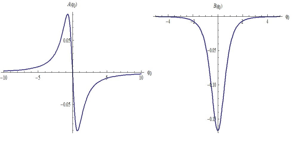
Figure 2: Plot of the functions $A$ and $B$ for $x_{1}=-1$.

We use this to simplify our formulas. For large values of $\beta$, one has that the maximum of the function $g$ occurs at

$$q_{0}\simeq\left(\frac{3\beta}{x_{1}^{2}}\right)^{\frac{1}{3}},$$ (79)

(which comes from Eq(73)) because in that limit

$$A\sim\frac{1}{\beta^{\frac{1}{3}}},\ B\sim\frac{-4x_{1}^{2}}{\beta^{\frac{4}{3}}}.$$ (80)

One then finds the dominant contribution (in the limit $\beta\longrightarrow\infty)$ to be given by

$$J_{0}\simeq\sqrt{\pi}\exp{\left(z_{0}\beta^{\frac{2}{3}}+z_{1}\beta^{\frac{4}{3}}\right)}.\ \left(z_{2}+z_{3}\beta^{\frac{2}{3}}\right)^{-\frac{1}{2}}$$ (81)

where the constants coefficients are given by

$$z_{0}=-x_{1}\left(\frac{3\beta}{x_{1}^{2}}\right)^{\frac{2}{3}},\ z_{1}=\frac{x_{1}^{2}}{2}\left(\frac{3\beta}{x_{1}^{2}}\right)^{\frac{4}{3}},\ z_{2}=-x_{1},\ z_{3}=x_{1}^{2}\left(\frac{3\beta}{x_{1}^{2}}\right)^{\frac{2}{3}}.$$ (82)

For the rest of our treatment, it appears more simple to write this result directly in terms of $q_{0}$ :

$$J_{0}=\sqrt{\pi}\left(-x_{1}+x_{1}^{2}q_{0}^{2}\right)^{-\frac{1}{2}}\exp{(-x_{1}q_{0}^{2}+\frac{1}{2}x_{1}^{2}q_{0}^{4})}.$$ (83)

One can now use the relation between $J_{n}$ and $J_{0}$. For example, for the first two following, one gets

$$\begin{split}J_{1}=\frac{\sqrt{\pi}}{2}q_{0}^{-1}&\left(-x_{1}+x_{1}^{2}q_{0}^{2}\right)^{-\frac{3}{2}}\left(1-4x_{1}q_{0}^{2}+2x_{1}^{2}q_{0}^{4}\right)\exp{(-x_{1}q_{0}^{2}+\frac{1}{2}x_{1}^{2}q_{0}^{4})},\\ J_{2}=\frac{\sqrt{\pi}}{4}x_{1}^{-1}q_{0}^{-4}&\left(-x_{1}+x_{1}^{2}q_{0}^{2}\right)^{-\frac{5}{2}}\\ &\times(1+2x_{1}q_{0}^{2}-10x_{1}^{2}q_{0}^{4}+22x_{1}^{3}q_{0}^{6}-16x_{1}^{4}q_{0}^{8}+4x_{1}^{5}q_{0}^{10})\exp{(-x_{1}q_{0}^{2}+\frac{1}{2}x_{1}^{2}q_{0}^{4})}.\end{split}$$ (84)

It should be noted that only the dominant term in the polynomial expression is relevant. This is justified by the fact the contribution coming from the coefficients $A$ and $B$ in Eq.(78) are ignored when computing the dominant term. This approach, which gives analytical formula, will be used later in the computation of the time scale where the classical solution begins separating from the mean value of the position operator for the coherent states studied here.

The second approach uses integration by parts. One has

$$J_{n}=\int_{-\infty}^{+\infty}dq\ q^{n}\ \exp{[g(q)]}.$$ (85)

If one introduces $u=q^{n}\ \exp{(x_{1}q^{2}-\frac{1}{6}x_{1}^{2}q^{4})}$ and $dv=\exp{(2\beta\ q)}dq$, one gets

$$\begin{split}J_{3}&=\frac{3}{x_{1}}J_{1}+\frac{3\beta}{x_{1}^{2}}J_{0},\\ J_{n+3}&=\frac{3n}{2\ x_{1}^{2}}J_{n-1}+\frac{3\beta}{x_{1}^{2}}J_{n}+\frac{3}{x_{1}}J_{n+1}\ ;n\geq 1.\end{split}$$ (86)

These relations are exact. They apply to small as well as to large values of $\beta$. They can be used in the following way. For a given value of $\beta$, one computes numerically $J_{0},J_{1}$ and $J_{2}$. All the others are then obtained by the preceding recursion formulas.

Finally, we use the mean value of the position operator given in Eq.(45). We first write explicitly the relation contained in Eq.(46)

$$C_{m,n}=\sum_{k=0}^{3m}\sum_{p=0}^{3n}\tilde{f}^{\star}_{m,k}\ \tilde{f}_{n,p}\ J_{k+p+1}.$$ (87)

The expressions of the $C_{m,n}$ (Eq.(87)) then leads to

$$\begin{split}\Omega_{0}&=J_{1},\\ \Omega_{1}=i\ &\Big{[}\left(-\tilde{f}_{1,0}+\tilde{f}^{\star}_{1,0}\right)J_{1}+\left(-\tilde{f}_{1,1}+\tilde{f}^{\star}_{1,1}\right)J_{2}\Big{]},\\ \Omega_{2}=-\frac{1}{2}&\ \Big{\{}\ \left(\tilde{f}_{2,0}+\tilde{f}^{\star}_{2,0}-2\tilde{f}^{\star}_{1,0}\tilde{f}_{1,0}\right)J_{1}\\ &+\Big{[}\tilde{f}_{2,1}+\tilde{f}^{\star}_{2,1}-2\left(\tilde{f}^{\star}_{1,0}\tilde{f}_{1,1}+\tilde{f}_{1,0}\tilde{f}^{\star}_{1,1}\right)\Big{]}J_{2}+\ \left(\tilde{f}_{2,2}+\tilde{f}^{\star}_{2,2}-2\tilde{f}^{\star}_{1,1}\tilde{f}_{1,1}\right)J_{3}\ \Big{\}},\\ \Omega_{3}=\frac{i}{6}&\ \Big{\{}\ \Big{[}\left(\tilde{f}_{3,0}-\tilde{f}^{\star}_{3,0}\right)+3\left(-\tilde{f}^{\star}_{1,0}\tilde{f}_{2,0}+\tilde{f}_{1,0}\tilde{f}^{\star}_{2,0}\right)\Big{]}J_{1}\\ &+\Big{[}\left(\tilde{f}_{3,1}-\tilde{f}^{\star}_{3,1}\right)+3\left(-\tilde{f}^{\star}_{1,0}\tilde{f}_{2,1}-\tilde{f}_{2,0}\tilde{f}^{\star}_{1,1}+\tilde{f}_{1,0}\tilde{f}^{\star}_{2,1}+\tilde{f}_{1,1}\tilde{f}^{\star}_{2,0}\right)\Big{]}J_{2}\\ &+\ \Big{[}\left(\tilde{f}_{3,2}-\tilde{f}^{\star}_{3,2}\right)+3\left(-\tilde{f}^{\star}_{1,0}\tilde{f}_{2,2}-\tilde{f}_{2,1}\tilde{f}^{\star}_{1,1}+\tilde{f}_{1,0}\tilde{f}^{\star}_{2,2}+\tilde{f}_{1,1}\tilde{f}^{\star}_{2,1}\right)\Big{]}J_{3}\\ &+\Big{[}\left(\tilde{f}_{3,3}-\tilde{f}^{\star}_{3,3}\right)+3\left(-\tilde{f}^{\star}_{1,1}\tilde{f}_{2,2}+\tilde{f}_{1,1}\tilde{f}^{\star}_{2,2}\right)\Big{]}J_{4}\Big{\}},\\ &\cdots\end{split}$$ (88)

On the other hand, the classical trajectories are analytical functions of time. Rather than relying on their periodic character, we shall consider the equation of motion

$$q^{\prime\prime}(t)-\mu q^{3}(t)-\sigma q^{5}(t)=0,$$ (89)

with $\mu=-\frac{4}{3}\omega^{2}x_{1}^{3}$ and $\sigma=\frac{1}{3}\omega^{2}x_{1}^{4}$.
One sees that a power series solution of the form

$$q_{class}(t)=\sum_{i=0}^{\infty}A_{i}.(\omega t)^{i}$$ (90)

leads to the following relation between the coefficients

$$\begin{split}A_{2}&=\frac{1}{6}(A^{5}_{0}-4A^{3}_{0});\\ A_{3}&=\frac{1}{18}(5A_{1}A^{4}_{0}-12A_{1}A^{2}_{0});\\ A_{4}&=\frac{1}{216}(5A_{0}^{9}-32A^{7}_{0}+48A^{5}_{0}+60A^{2}_{1}A^{3}_{0}-72A^{2}_{1}A_{0});\\ A_{5}&=\frac{1}{1080}(85A_{1}A^{8}_{0}-432A_{1}A^{6}_{0}+432A_{1}A^{4}_{0}+180A^{3}_{1}A^{2}_{0}-72A^{3}_{1});\\ \cdots\end{split}$$ (91)

The trajectories will be identical if the equations Eq.(91) are still satisfied when the constants $A(i)$ are replaced by the coefficients $\Omega_{i}$. For our case, this amount to the vanishing of the following quantities

$$\Big{\lvert}\frac{q_{cl}(t)-q_{moy}(t)}{q_{cl}(t)}\Big{\rvert}\approx\varepsilon\ll 1$$ (92)

$$\lvert\omega t\rvert\leq\varepsilon^{\frac{1}{2}}\Big{\lvert}\frac{x_{1}^{2}}{f(x_{1},\beta)}\Big{\rvert}^{\frac{1}{2}}$$ (93)

$$\begin{split}f(x_{1},\beta)=&6x_{1}\Big{[}-4\gamma^{2}\left(3x_{1}\beta^{4}\right)^{\frac{1}{3}}-\left(9x_{1}^{2}\beta^{2}\right)^{\frac{1}{3}}\left(\beta^{2}+\gamma^{2}\right)-2\beta^{2}\gamma^{2}+x_{1}\left(\beta^{2}-\gamma^{2}\right)\Big{]}\\ &+\pi^{2}\exp{\Big{[}4\left(-x_{1}q_{0}^{2}+\frac{1}{2}x_{1}^{2}q_{0}^{4}\right)\Big{]}}-4\pi x_{1}^{2}\exp{\Big{[}2\left(-x_{1}q_{0}^{2}+\frac{1}{2}x_{1}^{2}q_{0}^{4}\right)\Big{]}}.\end{split}$$ (94)

$$\lvert\omega t\rvert\leq\varepsilon^{\frac{1}{2}}\Big{\lvert}\frac{6\Omega_{0}}{\Omega_{0}^{5}-4\Omega_{0}^{3}-6\Omega_{2}}\Big{\rvert}^{\frac{1}{2}}$$ (95)

This will hold true for times very small compared to the intrinsic frequency of the system.

Conclusions

In this paper, we devised a general method for the computation of the quantum trajectories of generalized coherent states in the supersymmetric context. Our approach was successfully applied to the harmonic oscillator. We then applied it to one of the simplest superpotentials whose coherent states are normalizable. We found for this specific case the timescale after which the classical and quantum trajectories begin having significant differences. Although technical difficulties arise, our approach can be used to analyze the product of the uncertainties in physical position and momentum operators and see how it evolves in view of the absolute bound given by the Heisenberg inequality.

Some mathematical issues have not been addressed here. One of them is the convergence of the series obtained for the position operator mean value. This is a very difficult point since we do not have the explicit formula for the coefficient $\Omega_{l}$. But in principle, since the problem is well posed, the results should be meaningful.
The method we followed here gives the position as an analytic series in time. One has to sum a finite number of terms to obtain an approximation. Such a finite sum is polynomial. This explains why after some time the graph goes to infinity; this simply means we are out of the domain where the approximation is valid.

The SUSY structure has been extensively used (see Eq.(34), Eq.(35),Eq.(36)). This culminated in the recurrence formula of Eq.(39) which gives the nth contribution to the wave function. The superpotential $x(q)$ appears many times because it is the result of the commutation relations between the operators A and $A^{\dagger}$ (Eq.(20)). The coefficients $C_{m,n}$ are not easy to find analytically, even for simple superpotentials like the one we studied here. We devised recipes which can tackle this successfully. This was the case of the saddle point approximation whose domain of validity was explicitly given.
It should be emphasized that the coherent states studied here were not constructed as superposition of the quantum energy eigenstates . So it does not make sense to question its normalisability. It is normalizable in the Heisenberg picture ; since the evolution operator which relates it to the Schr0dinger picture is unitary ; its time evolved equivalent has the same norm.

Let us finish with some considerations concerning formal remarks which can be misleading. It has been argued in the case of coherent states defined as infinite superpositions of energy eigenstates that in most cases the wave function so obtained is only formal i.e it does not converge when considering for example imaginary times. First, we have no reason to turn to imaginary times in this work. Secondly, the definition of coherent states adopted here is a priori different so that there is no reason the claim made above, if true , should apply here.

To finish, our work can be seen as a particular illustration of the Ehrenfest theorem i.e in most general cases, the classical and quantum trajectories are not the same.

Appendix : The Harmonic Oscillator

We give here the results obtained by our treatment when applied to the harmonic oscillator. The functions $f_{n}$ are polynomial

$$f_{n}(q,\alpha)=\sum_{k=0}^{n}\tilde{f}_{n,k}(\alpha)q^{k};\tilde{f}_{0,0}=\tilde{f}_{0,0}^{\star}=1.$$ (96)

The coefficients we need are given by the following integrals

$$\begin{split}C_{m,n}&=\sum_{k=0}^{m}\sum_{p=0}^{n}\int_{-\infty}^{+\infty}dq.q^{k+p+1}\tilde{f}^{\star}_{m,k}(\alpha)\tilde{f}_{n,p}(\alpha)\psi_{H}^{\star}(q,\alpha)\psi_{H}(q,\alpha)\ ;\\ C_{m,n}&=\sum_{k=0}^{m}\sum_{p=0}^{n}\int_{-\infty}^{+\infty}dq.q^{k+p+1}\tilde{f^{\star}}_{m,k}(\alpha)\tilde{f}_{n,p}(\alpha)\exp{(2\beta q-q^{2})}\ \end{split}$$ (97)

where, by definition, the coefficient $\beta$ is given by

$$2\beta=\sqrt{2}(\alpha+\alpha^{\star}).$$ (98)

We have fewer recursion relations

$$\begin{split}\tilde{f}_{n+1,0}&=-\tilde{f}_{n,2}-\sqrt{2}\alpha\tilde{f}_{n,1}-\alpha^{2}\tilde{f}_{n,0};\\ \tilde{f}_{n+1,l}&=-\frac{1}{2}(l+1)(l+2)\tilde{f}_{n,l+2}-\sqrt{2}\alpha(l+1)\tilde{f}_{n,l+1}+(l-\alpha^{2})\tilde{f}_{n,l}+\sqrt{2}\alpha\tilde{f}_{n,l-1};\\ \tilde{f}_{n+1,n-1}&=-\sqrt{2}\alpha n\tilde{f}_{n,n}+(n-1-\alpha^{2})\tilde{f}_{n,n-1}+\sqrt{2}\alpha\tilde{f}_{n,n-2};\\ \tilde{f}_{n+1,n}&=(n-\alpha^{2})\tilde{f}_{n,n}+\sqrt{2}\alpha\tilde{f}_{n,n-1};\\ \tilde{f}_{n+1,n+1}&=\sqrt{2}\alpha\tilde{f}_{n,n}.\end{split}$$ (99)

Our coefficients $C_{m,n}$ are given by integrals of the product of an exponential and a power of the variable $q$ (See Eq.(97)). Actually, the only thing one needs is

$$J_{0}=\int_{-\infty}^{+\infty}dq.\exp{(-q^{2}+2\beta q)}\,$$ (100)

because

$$\int_{-\infty}^{+\infty}dq.q^{k+p+1}\exp{(2\beta q-q^{2})}\ =\sqrt{\pi}\ \frac{1}{2^{k+p+1}}\ \frac{\partial^{k+p+1}}{\partial\beta^{k+p+1}}\Big{[}\exp{(\beta^{2})}\Big{]}.$$ (101)

The coefficients can now be recast in the form

$$C_{m,n}=\sqrt{\pi}\exp{\beta^{2}}\sum_{k=0}^{m}\sum_{p=0}^{n}\tilde{f^{\star}}_{m,k}(\alpha)f_{n,p}(\alpha)\ \frac{1}{2^{k+p+1}}\ P_{k+p+1}(\beta).$$ (102)

The polynomials $P_{s}$ are defined by the property

$$\frac{d^{s}}{d\beta^{s}}\exp{(\beta^{2})}=\exp{(\beta^{2})}\ P_{s}(\beta).$$ (103)

One readily finds that they obey the recursion relations

$$P_{s+1}(\beta) = 2\beta P_{s}(\beta)+\frac{d}{d\beta}P_{s}(\beta);$$ (104)

$$P_{0}(\beta) = 1.$$

Let us now compare the quantum and the classical trajectories for the harmonic oscillator using our approach.
For the quantum behavior on the other side, one finds

$$\begin{split}\Omega_{0}&=\sqrt{\pi}\ \beta\ \exp{(\beta^{2})},\\ \Omega_{1}&=i\sqrt{\frac{\pi}{2}}\ \beta\ \exp{(\beta^{2})},\\ \Omega_{2}&=-\frac{1}{2}\sqrt{\pi}\ \exp{(\beta^{2})},\\ \Omega_{3}&=-\frac{i}{6}\sqrt{\frac{\pi}{2}}\ \beta\ \exp{(\beta^{2})},\\ \Omega_{4}&=\frac{1}{24}\sqrt{\pi}\ \exp{(\beta^{2})},\\ &\cdots\end{split}$$ (105)

The following ratios

$$\begin{split}&\frac{\Omega_{2}}{\Omega_{0}}=-\frac{1}{2},\ \frac{\Omega_{4}}{\Omega_{0}}=\frac{1}{24},\ \frac{\Omega_{6}}{\Omega_{0}}=-\frac{1}{720},\ \frac{\Omega_{8}}{\Omega_{0}}=\frac{1}{40320},\ \frac{\Omega_{10}}{\Omega_{0}}=-\frac{1}{3628800},\ \cdots\\ &\frac{\Omega_{3}}{\Omega_{1}}=-\frac{1}{6},\ \frac{\Omega_{5}}{\Omega_{1}}=\frac{1}{120},\ \frac{\Omega_{7}}{\Omega_{1}}=-\frac{1}{5040},\ \frac{\Omega_{9}}{\Omega_{1}}=\frac{1}{362880},\ \cdots\end{split}$$ (106)

drives us to conclude that the behavior of the classical trajectory given in Eq.(48) is recovered, at least in the lowest order. One can go to higher order and verify this still works.

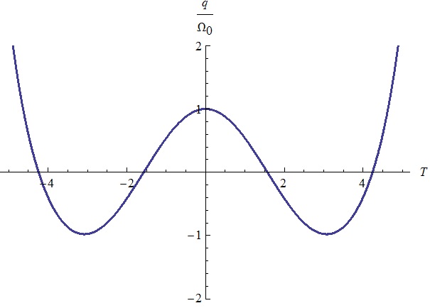
Figure 3: Plot of $q(t)$ for the Harmonic Oscillator, for the value $\alpha=10$, an approximation to the 8th order.

The same calculation done in section 3 for our toy model shows the plot of $q(t)$ below. The Figure 3 shows a kind of oscillation for a small interval of time.
We were able to plot the function $q(t)$ for the parameters $x_{1}=-1$ and $\beta=\frac{4}{3}$. But this was not sufficient to completely determine the coherent state’s parameter $\alpha$, the unique information was $Re(\alpha)=\frac{2\sqrt{2}}{3}$ and $Im(\alpha)\leq 0$. The ”kind of oscillations” appeared for the smallest values of $Im(\alpha)$ and the smallest times, as shown in the Figure 3.

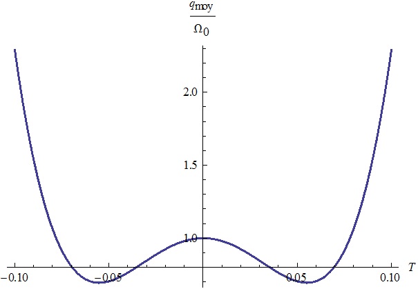
Figure 4: Plot of $q(t)$ for the Toy for the values $\alpha=\frac{100\sqrt{2}}{3}-\frac{i}{10000}$ and $x_{1}=-1$.The calculation was done to the 4th order.

References

• [1] Molski, M., J. Phys. A : Math. Theor. 42 165301 (2009).
• [2] Mikulski, D., Konarski, J., Krzysztof, E., Molsky, M., Kabaciński, S. J., Math. Chem. (2015) 53 : 2018.
• [3] Sabi Takou D., Avossevou G. Y. H., Kounouhewa. 10.1515/Phys-2015-0021.
• [4] Mikulski, D., Molski, M., Konarski, J., Krzysztof, E., Journal of Mathematical Chemistry 52(1) - January 2014. J. Math. Chem. (2014).
• [5] Mikulski, D., Konarski, J., Krzysztof, E., Molsky, M., Annals of Physics 339 : 122-134- December 2013.
• [6] Pawlowski, J., Szumniak, P., Bednarek, S., Phys. Rev. B 94, 155407-2016.
• [7] Clark, L.A., Stokes, A., Beige, A., Phys. Rev. A94, 023840 (2016).
• [8] Popov, D., Shi-Hai Dong, Pop, N., Sajfert, V., Şimon, S., Annals of Physics, Volume 39, December 2013, Pages 122-134.
• [9] Drăgănescu, G. E., Physica Scripta, Volume 2013, T153, March 23rd, 2013.
• [10] Yahiaoui, S. A., Bentaiba, M., Journal of Physics A : Mathematical and Theoretical, Volume 45(44), January 2012.
• [11] Ruby, V. C., Senthilvelan, M., J. Math. 51, 052106 (2010).
• [12] Malkiewicz, P., Affine Coherent States in Quantum Cosmology. ArXiv : 1512.04304v1[gr-qc].
• [13] De Lima Rodrigues, R., De Lima, A. F., De Araújo Ferreira, K., Vaidya, A. N., ArXiv : hep-th/0205175v7.
• [14] Bergeron, H., Gazeau, J. P., Youssef, A. ArXiv : quant-ph/1007.3876.
• [15] Balondo Iyela, D., Govaerts, J., Hounkonnou, M. N., Journal of Mathematical Physics 54, 093502 (2013).
• [16] Antoine, J. P., Gazeau, J. P., Monceau, P., Klauder, J. R., Penson, K. A., Journal of Mathematical Physics, Volume 42, 2349(2001).
• [17] Aremua, I., Gazeau, J. P., Hounkonnou, M. N., Journal of Physics A: Mathematical and Theoretical 45(33). November 2011.
• [18] Gazeau, J. P., delOlmo, M. A. , Annals of Physics Volume 330, March 2013, Pages 220-245.
• [19] Bergeron, H., Gazeau, J. P., Siegl, P., Youssef, A., EPL (Europhysics Letters), Volume 92, Number 6.
• [20] El Baz, M., Fresneda, R., Gazeau, J. P., Hassouni, Y., Journal of Physics A: Mathematical and Theoretical Volume 43, Number 38.
• [21] Hounkonnou, M., N., Arjikab, S., Baloïtchac, E., Journal of Mathematical Physics 55, 123502 (2014).
• [22] Bergeron, H., Siegl, P., Youssef, A., Journal of Physics A: Mathematical and Theoretical, Volume 45, Number 24.
• [23] Angelova, M., Hertz, A., Hussin, V., J. Phys. A: Math. Theor. 45 244007(2012), ArXiv: 1111.1974v3 [math-ph].
• [24] Nieto, M., M., 1997, ArXiv : quant-ph/9708012.
• [25] Perelomov, A.M. (1986) Generalized Coherent States and their Applications, Springer-Verlag, Berlin.
• [26] Klauder, J., R., Penson, K., A., JM 2001, Phys.Rev.A. 64013817.
• [27] Kuang, L.M., Wang, F.B., Zhou, Y.G. (1993), Phys. Lett. A, 183, 1.
• [28] Gazeau, J.-P., Maquet, A. (1979), Phys. Rev. A, 20, 727.
• [29] Castañeda, J. A., Hernández, M. A., Jáuregui, R. (2008), Phys. Rev. A, 78, 78.
• [30] Gazeau, J., -P. Coherent States in Quantum Physics, 2009, Wiley-VCh Verlag GmbH & Co. KGaA, Weinheim.
• [31] Benedict, M.G, Molnar, B. (1999), Phys. Rev. A, 60, R1737.
• [32] Molnar, B., Benedict, M.G, Bertrand, J. (2001)l, J. Phys. A : Math. Gen., 34, 3139.
• [33] Kastrup, H.A. (2007) , Ann. Phys. (Leipzig), 7–8, 439.
• [34] Kuang, L.M., Wang, F.B., Zhou, Y.G. (1994), J. Mod. Opt., 41, 1307.
• [35] Nieto, M.M., Simmons, Jr., L.M. (1987), Phys. Rev. Lett., 41, 207.
• [36] Antoine, J.-P., Gazeau, J.-P., Monceau, P., Klauder, J.R., Penson, K.A. (2001)l, J. Math. Phys., 42, 2349.
• [37] Barut, A.O. and Girardello, L. (1971), Commun. Math. Phys., 21, 41.
• [38] Klauder, J.R., Skagerstam, B.S. (eds) (1985) Coherent states. Applications in physics and mathematical physics, World Scientific Publishing Co., Singapore.
• [39] Garcia de Leon, P., Gazeau, J.-P., Quéva, J. (2008), Phys. Lett. A, 372, 3597.
• [40] Cooper, F., Khare, A., Sukhatme, U., Phys. Rep. 251, 267-385.
• [41] Khare, A., Sukhatme, U., P., 1993, J. Phys. A : Math. Gen. 26 L901-4.
• [42] Klauder, J., R., 1996, J. Phys. A : Math. Gen. 291, 293, 8.
• [43] Gerry, G., C., Kiefer, J., 1988, Phys. Rev. A 37 665-771.
• [44] Gazeau, J.-P. and Klauder, J.R. (1999), J. Phys. A : Math. Gen., 32, 123.
• [45] Khais, S., Levine, R. D., Phys. Rep. A 41 2301-05.
• [46] Gerry, G., C., 1985, Phys. Rev. A 31 2721-23.
• [47] Cooper, I., L 1992, Kiefer, J. Phys. A. : Math. Gen. 25 1671-83.