Static spin susceptibility in magnetically ordered states

Abstract

We report that special care is needed when longitudinal magnetic susceptibility is computed in a magnetically ordered phase, especially in metals. We demonstrate this by studying static susceptibility in both a ferromagnetic and an antiferromagnetic state in the random phase approximation to the two-dimensional Hubbard model on a square lattice. In contrast to the case in the disordered phase, a first derivative of the chemical potential (or the density) with respect to a magnetic field does not vanish in a magnetically ordered phase when the field is applied parallel to the magnetic moment. This effect is crucial and should be included when computing magnetic susceptibility in the ordered phase, otherwise an unphysical result would be obtained. In addition, consequently the magnetic susceptibility becomes different when computed at a fixed density and a fixed chemical potential in the ordered phase. In particular, we cannot employ magnetic susceptibility at a fixed chemical potential to describe a system with a fixed density even if the chemical potential is tuned to reproduce the correct density.

I Introduction

Spin susceptibility is a fundamental quantity to study the magnetic property of a system, and it is often computed in the so-called random phase approximation (RPA). While this approximation is usually good enough for a three-dimensional system, it may not be precise enough especially in a two-dimensional system. However, even in such a case, the susceptibility computed in the RPA is believed to capture at least qualitative properties of the system.

RPA susceptibility is frequently computed in a disordered phase, but it can also be computed in a magnetically ordered phase Izuyama et al. (1963); K. Ueda (1978). Moreover, as actually observed in high-temperature cuprates Mukuda et al. (2012), iron-based pnictides and chalcogenides Stewart (2011), and heavy fermion materials C. Pfleiderer (2009), the ordered phase sometimes coexists with superconductivity. Even in such a complicated situation, the RPA provides feasible computations of magnetic susceptibility H.-J. Lee and T. Takimoto (2012); Rowe et al. (2012).

Typically, RPA susceptibility is obtained by connecting a simple bubble (or ladder) of noninteracting particle-hole excitations with the electron-electron interaction, that is, its functional form is given typically by

$$\chi\propto(1-\chi_{0}g)^{-1}\chi_{0}\,,$$ (1)

where $g$ is the interaction strength and $\chi_{0}$ is the susceptibility in the noninteracting case; $\chi$, $\chi_{0}$, and $g$ can be matrices. In a magnetic phase, $\chi_{0}$ is computed by using the quasiparticle propagator in the ordered phase, and also by considering possible umklapp contributions to the susceptibility when the translational symmetry is broken by a magnetic order. Such a procedure indeed yields the correct result of transverse magnetic susceptibility Izuyama et al. (1963); K. Ueda (1978); Schrieffer et al. (1989); A. V. Chubukov and D. M. Frenkel (1992); A. P. Kampf (1994); Knolle et al. (2010); H.-J. Lee and T. Takimoto (2012); Rowe et al. (2012), but special care is needed for longitudinal magnetic susceptibility, which is not well recognized Sokoloff (1969); Schrieffer et al. (1989); A. P. Kampf (1994); Knolle et al. (2010); Rowe et al. (2012).

Spin rotational symmetry is broken in a magnetically ordered phase. As a result, the chemical potential (or the density) is no longer a quadratic function of a magnetic field when the field is applied parallel to the magnetic moment. A first derivative of the chemical potential (or the density) then becomes finite. Hence this effect should be considered on an equal footing when we compute magnetic susceptibility, because the magnetic susceptibility is a linear-response quantity of a magnetic field.

In this paper, we show how important the contribution of the first derivative of the chemical potential (or the density) is to compute longitudinal susceptibility in a magnetically ordered phase, which we exemplify by employing the two-dimensional Hubbard model for both a ferromagnetic and an antiferromagnetic state. Since the RPA is equivalent to the mean-field approximation or the saddle-point approximation, we can directly compute the magnetic susceptibility in mean-field theory for the Hubbard model. We provide the correct expression of the static susceptibility in the RPA as well as results when the first derivative of the chemical potential (or the density) is neglected. In addition, we point out that the longitudinal magnetic susceptibility is different when computed at a fixed density and a fixed chemical potential in a magnetically ordered phase. Consequently, when the density is fixed, the susceptibility obtained at a fixed chemical potential cannot be applicable even if the chemical potential is tuned to reproduce the correct density.

This paper is organized as follows. In Sec. II we present the model and derive the self-consistency equations for both a ferromagnetic and an antiferromagnetic phase. The corresponding magnetic susceptibility is computed in Secs. III and IV, respectively. We show in Sec. V that the susceptibility for a fixed chemical potential is reproduced in a conventional diagrammatic approach. Concluding remarks are given in Sec. VI.

II Model and self-consistency equations

To exemplify our issue, we employ the two-dimensional Hubbard model on a square lattice,

$$\mathcal{H}=-\sum_{i,j,\sigma}t_{ij}c^{\dagger}_{i\sigma}c_{j\sigma}+U\sum_{j}n_{j\uparrow}n_{j\downarrow}+\mathcal{H}_{z},$$ (2)

where the transfer integrals $t_{ij}$ are finite between the first- ($t$) and second- ($t^{\prime}$) neighbor sites and otherwise zero; $U$ represents the on-site Coulomb repulsion. $\mathcal{H}_{z}$ is the Zeeman term, for which we consider a static and uniform (staggered) magnetic field when we compute longitudinal magnetic susceptibility in a ferromagnetic (an antiferromagnetic) state. That is, it is described as

$$\mathcal{H}_{z}=-h\sum_{j}\frac{1}{2}(n_{j\uparrow}-n_{j\downarrow})e^{{\rm i}{\bf q}\cdot{\bf r}_{j}}$$ (3)

with ${\bf q}=0$ [${\bf q}={{\bf Q}}\equiv(\pi,\pi)$]. Here $h$ is an effective magnetic field given by $h=\mathfrak{g}\mu_{B}H$; $\mathfrak{g}$ is a $g$ factor, $\mu_{B}$ the Bohr magneton, and $H$ an external magnetic field. The magnetic field is infinitesimally small and we take the limit of $h\rightarrow+0$ when we compute the susceptibility.

Since the RPA is equivalent to the mean-field approximation, we compute the RPA susceptibility in mean-field theory. Defining the magnetization and the density operator as

$$m_{j}=\frac{1}{2}(n_{j\uparrow}-n_{j\downarrow})\,,$$ (4)

$$n_{j}=n_{j\uparrow}+n_{j\downarrow}\,,$$ (5)

respectively, the interaction term is written as $n_{j\uparrow}n_{j\downarrow}=\frac{1}{4}n_{j}n_{j}-m_{j}m_{j}$. The density is assumed to be uniform and is given by $n=\langle n_{j}\rangle$ whereas the magnetization $\langle m_{j}\rangle$ is uniform in the ferromagnetic state and staggers with a wavevector ${\bf q}={\bf Q}$ in the antiferromagnetic state. In mean-field theory the interaction term is decoupled as

$$n_{j\uparrow}n_{j\downarrow}\rightarrow\frac{n}{2}n_{j}-2\langle m_{j}\rangle m_{j}-\frac{1}{4}n^{2}+\langle m_{j}\rangle^{2}\,,$$ (6)

and self-consistency equations for $n$ and $\langle m_{j}\rangle$ are obtained by minimizing the free energy.

In the ferromagnetic state, $\langle m_{j}\rangle$ is independent of $j$, i.e., $\langle m_{j}\rangle=m$. The self-consistency equations are given by

$$n=\frac{1}{N}\sum_{{\bf k}}\left[f\left(\xi_{{\bf k}}-Um-\frac{h}{2}\right)+f\left(\xi_{{\bf k}}+Um+\frac{h}{2}\right)\right],$$ (7)

$$m=\frac{1}{2N}\sum_{{\bf k}}\left[f\left(\xi_{{\bf k}}-Um-\frac{h}{2}\right)-f\left(\xi_{{\bf k}}+Um+\frac{h}{2}\right)\right]\,.$$ (8)

Here

$$\xi_{{\bf k}}=-2t(\cos k_{x}+\cos k_{y})-4t^{\prime}\cos k_{x}\cos k_{y}+\frac{Un}{2}-\mu\,,$$ (9)

and $f$, $\mu$, and $N$ are the Fermi distribution function, the chemical potential, and the total number of lattice sites, respectively, and the summation of ${\bf k}$ is taken over the first Brillouin zone.

In the case of the antiferromagnetic state, the magnetization is described by $\langle m_{j}\rangle=m_{{\bf Q}}e^{{\rm i}{\bf Q}\cdot{\bf r}_{j}}$. Here $m_{{\bf Q}}$ is the staggered magnetization, which is the order parameter of antiferromagnetism. The self-consistency equations are given by

$$n=\frac{2}{N}\sideset{}{{}^{\prime}}{\sum}_{{\bf k}}\left[f(E^{+}_{{\bf k}})+f(E^{-}_{{\bf k}})\right],$$ (10)

$$m_{{\bf Q}}=-\frac{1}{N}\sideset{}{{}^{\prime}}{\sum}_{{\bf k}}\frac{Um_{{\bf Q}}+\frac{h}{2}}{D_{{\bf k}}}\left[f(E^{+}_{{\bf k}})-f(E^{-}_{{\bf k}})\right],$$ (11)

where the summation of ${\bf k}$ is taken over the magnetic Brillouin zone, namely $|k_{x}|+|k_{y}|\leq\pi$, and

$$E^{\pm}_{{\bf k}}=\xi^{+}_{{\bf k}}\pm D_{{\bf k}}\,,$$ (12)

$$\xi^{\pm}_{{\bf k}}=\frac{1}{2}(\xi_{{\bf k}}\pm\xi_{{\bf k}+{\bf Q}})\,,$$ (13)

$$D_{{\bf k}}=\sqrt{(\xi^{-}_{{\bf k}})^{2}+\left(Um_{{\bf Q}}+\frac{h}{2}\right)^{2}}\,.$$ (14)

A comprehensive mean-field analysis of the Hubbard model Igoshev et al. (2010) clarified the parameter region where ferromagnetic phases with ${\bf q}=0$ and antiferromagnetic phases with ${\bf q}={\bf Q}$ are stabilized. Referring to Ref. Igoshev et al., 2010, we fix $U=3t$ and choose $t^{\prime}=-0.45t$ and $n=0.2$ to describe the ferromagnetic state, and $t^{\prime}=-0.2t$ and $n=1.1$ for the antiferromagnetic state. Our conclusions, however, do not depend on the choice of parameters as long as the ferromagnetic (or antiferromagnetic) phase is stabilized. In the following, we set $t=1$ and measure all quantities with the dimensions of energy in units of $t$.

III Uniform susceptibility in the ferromagnetic state

The longitudinal magnetic susceptibility is obtained in the RPA by taking a first derivative with respect to a field in Eqs. (7) and (8), and then by taking the limit of $h\rightarrow+0$. One would assume that a first derivative of $\mu$ (or $n$) with respect to a field should vanish in the limit of $h\rightarrow+0$. This is actually correct at least in the disordered phase. As a result, the longitudinal susceptibility, which is defined by $\frac{\partial m}{\partial h}\left|{}_{h\to+0}\right.$, is obtained as

$$\tilde{\chi}({\bf 0})=\frac{1}{4}\frac{\chi_{\uparrow}+\chi_{\downarrow}}{1-\frac{U}{2}(\chi_{\uparrow}+\chi_{\downarrow})}\,,$$ (15)

where

$$\chi_{\uparrow(\downarrow)}=-\frac{1}{N}\sum_{{\bf k}}f^{\prime}(\xi_{{\bf k}}\mp Um)$$ (16)

and $f^{\prime}$ is the first derivative with respect to energy.

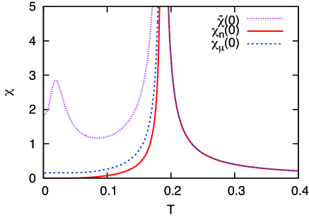
Figure 1: Longitudinal magnetic susceptibility as a function of temperature at a fixed density; $n=0.2,t^{\prime}=-0.45$, and $U=3$. The Curie temperature is $T_{\rm FM}=0.187$, below which the ferromagnetic moment develops. $\tilde{\chi}({\bf 0})$ is obtained from Eq. (15) and correct only in $T>T_{\rm FM}$. $\chi_{n}({\bf 0})$ is given by Eq. (17) and correct in the whole temperature region. For $\chi_{\mu}({\bf 0})$ [Eq. (19)], the chemical potential is tuned at each temperature to reproduce the fixed density $n=0.2$. $\chi_{\mu}({\bf 0})$ provides the correct result only in $T>T_{\rm FM}$.

The temperature ($T$) dependence of $\tilde{\chi}({\bf 0})$ is shown in Fig. 1. With decreasing $T$, $\tilde{\chi}({\bf 0})$ grows and diverges at the Curie temperature $T_{\rm FM}$ ($=0.187$). Below $T_{\rm FM}$, ferromagnetic order $m$ develops. The value of $m$ is determined by the self-consistency equations Eqs. (7) and (8). As expected, $\tilde{\chi}({\bf 0})$ is suppressed below $T_{\rm FM}$. However, it is enhanced at lower temperature inside the ferromagnetic state. This dependence is obviously unphysical and originates from the wrong assumption that the chemical potential should remain a quadratic function with respect to a field inside the ferromagnetic state. To show this, we plot $\Delta\mu(T,h)\equiv\mu(T,h)-\mu(T,0)$ in Fig. 2. The chemical potential $\mu$ has a quadratic dependence of $h$ in the vicinity of $h=0$ in the disordered phase because of the spin-rotational symmetry of the system. Its curvature around $h=0$ becomes larger upon approaching $T_{\rm FM}$ and becomes infinite just at $T_{\rm FM}$. Below $T_{\rm FM}$, a linear term emerges with a singularity at $h=0$. The emergence of the linear term is due to the breaking of the spin rotational symmetry, that is, the system has a different response when an infinitesimally small field is applied parallel and anti-parallel to the direction of the ferromagnetic moment. Therefore the emergent linear term in $h$ is crucially important to describe the response in the ordered phase and Eq. (15) is valid only in the disordered phase where $m=0$. While $\tilde{\chi}({\bf 0})$ is enhanced below $T\lesssim 0.05$ in Fig. 1 for the present choice of the parameters, it could diverge inside the ferromagnetic phase, especially when $U$ is chosen to be a larger value.

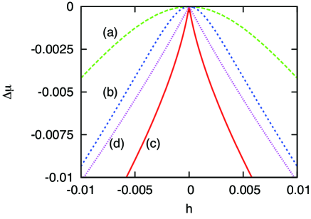
Figure 2: $h$ dependence of the chemical potential for several choices of temperatures: (a) $T=1.1T_{\rm FM}$, (b) $T=1.04T_{\rm FM}$, (c) $T=0.99T_{\rm FM}$, and (d) $T=0.9T_{\rm FM}$.

III.1 Fixed density

We first consider the situation where the density is fixed. In order to get the correct RPA susceptibility inside the ordered phase, a first derivative of $\mu$ should be kept when differentiating Eqs. (7) and (8) with respect to $h$. Solving coupled equations, we obtain

$$\chi_{n}({\bf 0})=\left.\frac{\partial m}{\partial h}\right|_{h\to+0}=\frac{\chi_{\uparrow}\chi_{\downarrow}}{\chi_{\uparrow}+\chi_{\downarrow}-2U\chi_{\uparrow}\chi_{\downarrow}}\,,$$ (17)

$$\left.\frac{\partial\mu}{\partial h}\right|_{h\to+0}=-\frac{1}{2}\frac{\chi_{\uparrow}-\chi_{\downarrow}}{\chi_{\uparrow}+\chi_{\downarrow}-2U\chi_{\uparrow}\chi_{\downarrow}}\,.$$ (18)

In the disordered phase, we have $\chi_{\uparrow}=\chi_{\downarrow}$. Hence Eq. (17) is reduced to Eq. (15) and $\left.\frac{\partial\mu}{\partial h}\right|_{h\to+0}=0$. However, inside the ferromagnetic phase, it is clear that the functional form of Eq. (17) is very different from Eq. (15) and in addition $\left.\frac{\partial\mu}{\partial h}\right|_{h\to+0}$ becomes finite. We plot the temperature dependence of $\chi_{n}({\bf 0})$ in Fig. 1. $\chi_{n}({\bf 0})$ is suppressed monotonically inside the ferromagnetic phase with decreasing temperature. This is because the system becomes less susceptible to an infinitesimally small field parallel to the magnetic moment when the magnetic moment grows with decreasing temperature. The enhancement of Eq. (15) inside the ferromagnetic phase (Fig. 1), therefore should be an artifact due to the discarding of the contribution from $\left.\frac{\partial\mu}{\partial h}\right|_{h\to+0}$. As already implied in Fig. 2, the contribution of $\left.\frac{\partial\mu}{\partial h}\right|_{h\to+0}$ is indeed sizable below $T_{\rm FM}$. The temperature dependence of $\left.\frac{\partial\mu}{\partial h}\right|_{h\to+0}$ is plotted in Fig. 3. The quantity $\left.\frac{\partial\mu}{\partial h}\right|_{h\to+0}$ is zero down to $T=T_{\rm FM}$. It diverges at $T=T_{\rm FM}$ only on the side of low temperature and is suppressed with decreasing $T$, keeping a value comparable to $\chi_{n}({\bf 0})$ at low temperature (see also Fig. 1).

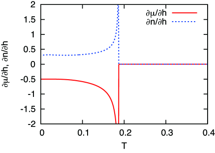
Figure 3: Temperature dependence of the first derivative of $\mu$ and $n$ with respect to a magnetic field $h$; $T_{\rm FM}=0.187$, $n=0.2,t^{\prime}=-0.45$, and $U=3$.

III.2 Fixed chemical potential

We now consider the situation where $\mu$ is fixed. In this case, we differentiate Eqs. (7) and (8) with respect to $h$ for a fixed $\mu$. We then obtain

$$\chi_{\mu}({\bf 0})=\left.\frac{\partial m}{\partial h}\right|_{h\to+0}=\frac{1}{4}\frac{\chi_{\uparrow}+\chi_{\downarrow}+2U\chi_{\uparrow}\chi_{\downarrow}}{1-U^{2}\chi_{\uparrow}\chi_{\downarrow}}\,,$$ (19)

$$\left.\frac{\partial n}{\partial h}\right|_{h\to+0}=\frac{1}{2}\frac{\chi_{\uparrow}-\chi_{\downarrow}}{1-U^{2}\chi_{\uparrow}\chi_{\downarrow}}\,.$$ (20)

Equation (19) is already known in the literature Izuyama et al. (1963); Moriya (1985).

In the disordered phase, we have $\chi_{\uparrow}=\chi_{\downarrow}$, yielding $\left.\frac{\partial n}{\partial h}\right|_{h\to+0}=0$ and $\chi_{\mu}=\chi_{n}=\tilde{\chi}$. Consequently, the magnetic susceptibility at a fixed density is the same as that at a fixed chemical potential in the disordered phase.

In the ordered phase, however, we have $\chi_{\uparrow}\neq\chi_{\downarrow}$, and $\left.\frac{\partial n}{\partial h}\right|_{h\to+0}$ becomes finite as shown in Fig. 3 and diverges at $T=T_{\rm FM}-0$. A comparison of Eqs. (17) and (19) should be made in the same condition, namely the same density and the same chemical potential. A physical quantity computed at a fixed chemical potential is frequently used to describe a system with a fixed density by tuning the chemical potential to reproduce the density. Following this standard procedure, we plot the temperature dependence of $\chi_{\mu}$ also in Fig. 1. Although the functional forms of Eqs. (17) and (19) are different, both provide similar results in the ordered phase. Nevertheless, in a strict sense, $\chi_{\mu}$ does not lead to the correct result $\chi_{n}$ when the density is fixed in the system. Conversely, $\chi_{\mu}$ [Eq. (19)] would provide the correct result when the chemical potential is fixed in the system (see Appendix). In this case, $\chi_{n}$ [Eq. (17)] is in turn not correct even if the density is tuned to reproduce the fixed chemical potential. The reason why the longitudinal magnetic susceptibility $\chi_{\mu}$ does not agree with $\chi_{n}$ in the magnetically ordered phase is that $\mu$ and $n$ are not symmetric in Eqs. (7) and (8), and thus the field dependences of $\mu$ and $n$ (see Fig. 3) are different from each other.

IV Staggered susceptibility in the antiferromagnetic state

The longitudinal staggered susceptibility is defined as $\left.\frac{\partial m_{{\bf Q}}}{\partial h}\right|_{h\to+0}$ where $h$ is a magnitude of a staggered field introduced in Eq. (3) with ${\bf q}={\bf Q}$. In the disordered phase, the spin rotational symmetry is preserved and thus $\mu$ and $n$ are quadratic functions of $h$ for a small $h$. In this case, we have $\left.\frac{\partial\mu}{\partial h}\right|_{h\to+0}=0$ and $\left.\frac{\partial n}{\partial h}\right|_{h\to+0}=0$. Thus we do not need to consider a first derivative of $\mu$ and $n$ with respect to $h$ in Eq. (11). The staggered susceptibility then becomes

$$\tilde{\chi}({\bf Q})=\frac{1}{2}\frac{\chi^{(0)}({\bf Q})}{1-U\chi^{(0)}({\bf Q})}\,,$$ (21)

where

$$\chi^{(0)}({\bf Q})=-\frac{1}{N}\sideset{}{{}^{\prime}}{\sum}_{{\bf k}}\frac{(\xi^{-}_{{\bf k}})^{2}}{D_{{\bf k}}^{3}}\left(f(E^{+}_{{\bf k}})-f(E^{-}_{{\bf k}})\right)$$

$$\hskip 34.1433pt-\frac{1}{N}\sideset{}{{}^{\prime}}{\sum}_{{\bf k}}\left(\frac{Um_{{\bf Q}}}{D_{{\bf k}}}\right)^{2}\left(f^{{}^{\prime}}(E^{+}_{{\bf k}})+f^{{}^{\prime}}(E^{-}_{{\bf k}})\right)\,,$$ (22)

and $m_{{\bf Q}}=0$ here. One might apply the formula Eq. (21) to the antiferromagnetic phase, employing $m_{{\bf Q}}$ and $n$ (or $\mu$) determined by solving the self-consistency equations Eqs. (10) and (11). The resulting $\tilde{\chi}({\bf Q})$ [Eq. (21)] is shown in Fig. 4 as a function of temperature. With decreasing $T$, $\tilde{\chi}({\bf Q})$ grows and diverges at the Néel temperature $T_{\rm AF}=0.380$. Just below $T_{\rm AF}$, $\tilde{\chi}({\bf Q})$ is suppressed as expected. However, it grows below $T\lesssim 0.2$ inside the antiferromagnetic phase. This apparently unphysical result originates from the wrong assumption that $\mu$ and $n$ would still be quadratic in $h$ in the magnetic phase. The enhancement of $\tilde{\chi}({\bf Q})$ could appear as its divergence at a certain temperature below $T_{\rm AF}$ when a larger value of $U$ is taken.

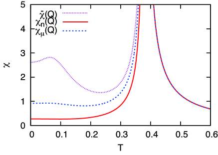
Figure 4: Longitudinal magnetic susceptibility as a function of temperature at a fixed density; $n=1.1,t^{\prime}=-0.2$, and $U=3$. The Néel temperature is $T_{\rm AF}=0.380$, below which the antiferromagnetic moment develops. $\tilde{\chi}({\bf Q})$ is obtained from Eq. (21) and correct only in $T>T_{\rm AF}$. $\chi_{n}({{\bf Q}})$ is given by Eq. (23) and correct in the whole temperature region. $\chi_{\mu}({\bf Q})$ [Eq. (30)] is computed in the condition of a fixed chemical potential; the chemical potential is tuned at each temperature to reproduce the correct density. The result $\chi_{\mu}({\bf Q})$ is, however, correct only in $T>T_{\rm AF}$.

Figure 5 shows $\Delta\mu=\mu(T,h)-\mu(T,0)$ as a function of $h$ for several choices of $T$. For $T>T_{\rm AF}$ we see $\left.\frac{\partial\mu}{\partial h}\right|_{h\to+0}=0$. However, below $T_{\rm AF}$, $\Delta\mu$ becomes singular at $h=0$ and acquires a linear dependence of $|h|$ around $h=0$. This effect is crucially important to obtain the correct RPA expression of the longitudinal magnetic susceptibility inside the magnetic phase. Because the correct expression depends on whether the density is fixed or the chemical potential is fixed, we present it below separately.

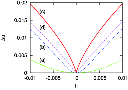
Figure 5: $h$ dependence of the chemical potential for several choices of temperatures: (a) $T=1.1T_{\rm AF}$, (b) $T=1.03T_{\rm AF}$, (c) $T=0.99T_{\rm AF}$, and (d) $T=0.9T_{\rm AF}$; $T_{\rm AF}=0.380$, $n=1.1,t^{\prime}=-0.2$ and $U=3$.

IV.1 Fixed density

For a fixed density $n$, we differentiate both Eqs. (10) and (11) with respect to $h$ and take the limit of $h\rightarrow+0$. Coupled equations of $\frac{\partial m}{\partial h}$ and $\frac{\partial\mu}{\partial h}$ are easily solved, yielding

$$\chi_{n}({\bf Q})=\left.\frac{\partial m}{\partial h}\right|_{h\to+0}=\frac{1}{2}\frac{\chi_{n}^{(0)}({\bf Q})}{1-U\chi_{n}^{(0)}({\bf Q})}\,,$$ (23)

$$\left.\frac{\partial\mu}{\partial h}\right|_{h\to+0}=-\frac{1}{2}\frac{a_{12}/a_{11}}{1-U\chi_{n}^{(0)}({\bf Q})}\,,$$ (24)

where

$$\chi_{n}^{(0)}({\bf Q})=\frac{a_{11}a_{22}-a_{12}a_{21}}{a_{11}}\,,$$ (25)

and

$$a_{11}=-\frac{2}{N}\sideset{}{{}^{\prime}}{\sum}_{{\bf k}}\left(f^{{}^{\prime}}(E^{+}_{{\bf k}})+f^{{}^{\prime}}(E^{-}_{{\bf k}})\right)\,,$$ (26)

$$a_{12}=\frac{2}{N}\sideset{}{{}^{\prime}}{\sum}_{{\bf k}}\frac{Um_{{\bf Q}}}{D_{{\bf k}}}\left(f^{{}^{\prime}}(E^{+}_{{\bf k}})-f^{{}^{\prime}}(E^{-}_{{\bf k}})\right)\,,$$ (27)

$$a_{21}=\frac{1}{2}a_{12}\,,$$ (28)

$$a_{22}=\chi^{(0)}({\bf Q})\,.$$ (29)

Here $h$ should be put zero in $E^{\pm}_{{\bf k}}$ and $D_{{\bf k}}$ [see Eqs. (12) and (14)]. The functional form of Eq. (23) is the same as Eq. (21), but $\chi^{(0)}_{n}({\bf Q})$ becomes identical to $\chi^{(0)}({\bf Q})$ only for $m_{{\bf Q}}=0$. $\chi_{n}({\bf Q})$ is plotted in Fig. 4 as a function of temperature. It is the same as Eq. (21) above $T_{\rm AF}$. Below $T_{\rm AF}$, $\chi_{n}({\bf Q})$ is suppressed monotonically with decreasing temperature as it should be. In Fig. 6 we plot $\left.\frac{\partial\mu}{\partial h}\right|_{h\to+0}$. It vanishes in the disordered phase, but becomes sizable in the magnetically ordered phase with divergence at $T=T_{\rm AF}$ on the side of low temperature.

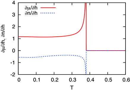
Figure 6: Temperature dependence of the first derivative of $\mu$ and $n$ with respect to a magnetic field $h$; $T_{\rm AF}=0.380$, $n=1.1,t^{\prime}=-0.2$, and $U=3$.

IV.2 Fixed chemical potential

We next fix the chemical potential and differentiate Eqs. (10) and (11) with respect to $h$. Taking the limit of $h\rightarrow+0$, we obtain

$$\chi_{\mu}({\bf Q})=\left.\frac{\partial m}{\partial h}\right|_{h\to+0}=\frac{1}{2}\frac{\chi_{\mu}^{(0)}({\bf Q})}{1-U\chi_{\mu}^{(0)}({\bf Q})}\,,$$ (30)

$$\left.\frac{\partial n}{\partial h}\right|_{h\to+0}=\frac{1}{2\left(1+\frac{U}{2}a_{11}\right)}\frac{a_{12}}{1-U\chi_{\mu}^{(0)}({\bf Q})}\,,$$ (31)

where

$$\chi^{(0)}_{\mu}({\bf Q})=a_{22}-\frac{U}{2}\frac{a_{12}a_{21}}{1+\frac{U}{2}a_{11}}\,.$$ (32)

The functional form of Eq. (30) is the same as Eq. (23) obtained at a fixed density. However, the expression of $\chi^{(0)}_{\mu}$ is very different from $\chi^{(0)}_{n}$ [Eq. (25)]. They become the same only in the disordered phase, where $m_{{\bf Q}}=0$ and thus $a_{12}=a_{21}=0$. Temperature dependence of $\chi_{\mu}({\bf Q})$ is shown in Fig. 4. Since the density is fixed in Fig. 4, the chemical potential is tuned to reproduce the correct density at each temperature, as is usually done. Below $T_{\rm AF}$, $\chi_{\mu}({\bf Q})$ is suppressed, but does not reproduce the correct result of $\chi_{n}({\bf Q})$. This wrong result originates from the naive assumption that the susceptibility obtained at a fixed chemical potential could be used for the system with a fixed density after tuning the chemical potential to reproduce the correct density. However, as we have obtained explicitly, the susceptibility at a fixed chemical potential [Eqs. (30) and (32)] is different from that at a fixed density [Eqs. (23) and (25)-(29)] in the magnetically ordered phase. Furthermore, as shown in Fig. 6, temperature dependence of $\left.\frac{\partial n}{\partial h}\right|_{h\to+0}$ is very different from $\left.\frac{\partial\mu}{\partial h}\right|_{h\to+0}$. Therefore the choice of $\chi_{n}$ and $\chi_{\mu}$ should be made carefully to describe the system appropriately. Reversely, if we wish to describe the system with a fixed chemical potential, the susceptibility $\chi_{\mu}({\bf Q})$ is the correct one and $\chi_{n}({\bf Q})$ [Eq. (23)] does not reproduce the correct result even if the density is tuned to reproduce the correct chemical potential at each temperature (see Appendix).

V Diagrammatic approach

It is natural to ask what kind of result is obtained when a diagrammatic approach is employed. The longitudinal magnetic susceptibility is defined by

$$\chi^{zz}({\bf q},{\rm i}\omega_{m})=\frac{1}{N}\int_{0}^{1/T}{\rm d}\tau{\rm e}^{{\rm i}\omega_{m}\tau}\langle T_{\tau}S^{z}({\bf q},\tau)S^{z}(-{\bf q},0)\rangle\,,$$ (33)

where $\omega_{m}=2m\pi T$ is the bosonic Matsubara frequency with $m$ being integer, $S^{z}({\bf q},\tau)={\rm e}^{\tau\mathcal{H}}S^{z}({\bf q}){\rm e}^{-\tau\mathcal{H}}$, and $S^{z}({\bf q})=\frac{1}{2}\sum_{{\bf k}\sigma}\sigma c_{{\bf k}\sigma}^{\dagger}c_{{\bf k}+{\bf q}\sigma}$.

In the disordered phase, $\chi^{zz}$ is given by the diagrams shown in Fig. 7 in the RPA. Hence we obtain

$$\chi^{zz}=\frac{1}{4}\left(\frac{\chi_{\uparrow}+\chi_{\downarrow}}{1-U^{2}\chi_{\uparrow}\chi_{\downarrow}}+\frac{2U\chi_{\uparrow}\chi_{\downarrow}}{1-U^{2}\chi_{\uparrow}\chi_{\downarrow}}\right)\,.$$ (34)

In the static case, we set ${\rm i}\omega_{m}=0$ and take ${\bf q}={\bf 0}$ and ${\bf Q}$ for the uniform and staggered susceptibility, respectively. We then obtain $\chi_{\uparrow}=\chi_{\downarrow}=\chi_{0}$, which is the same as Eq. (16) for the uniform susceptibility and Eq. (22) for the staggered susceptibility. Hence Eq. (34) is reduced to

$$\chi^{zz}=\frac{1}{2}\frac{\chi_{0}}{1-U\chi_{0}}\,,$$ (35)

and we reproduce the correct results Eqs. (15) and (21) in the disordered phase.

Figure 7: Diagrams of the longitudinal magnetic susceptibility for the Hubbard interaction. $\bar{\sigma}$ denotes the spin direction opposite to $\sigma$.

In the ordered phase, we may compute $\chi_{\uparrow(\downarrow)}$ by using the quasiparticle propagator. In the ferromagnetic phase, Eq. (34) then becomes the same as $\chi_{\mu}({\bf 0})$ [see Eq. (19) and Refs. Izuyama et al., 1963 and Moriya, 1985], but not $\chi_{n}(\bf 0)$ [Eq. (17)].

The situation is delicate in the antiferromagnetic phase. Although the translational symmetry is broken by the magnetic order, the umklapp components of the susceptibility such as $\langle T_{\tau}S^{z}({\bf q},\tau)S^{z}(-{\bf q}-{\bf Q},0)\rangle$ and $\langle T_{\tau}S^{z}({\bf q}+{\bf Q},\tau)S^{z}(-{\bf q},0)\rangle$, do not contribute to the longitudinal susceptibility Schrieffer et al. (1989). Hence one might think that the RPA susceptibility would be obtained simply by replacing the electron Green’s function with the Green’s function of the two-component field $\psi_{{\bf k}\sigma}^{\dagger}=(c_{{\bf k}\sigma}^{\dagger},c_{{\bf k}+{\bf Q}\sigma}^{\dagger})$; the summation of ${\bf k}$ is then restricted to the magnetic Brillouin zone. This kind of calculation is frequently seen in the literature Sokoloff (1969); Schrieffer et al. (1989); A. P. Kampf (1994); Knolle et al. (2010); Rowe et al. (2012). In this case, however, we obtain $\chi_{\uparrow}({\bf Q})=\chi_{\downarrow}({\bf Q})=\chi^{(0)}({\bf Q})$ [see Eq. (22)], which is the same as $\tilde{\chi}({\bf Q})$ and does not reproduce the correct result inside the antiferromagnetic phase as we have seen in Fig. 4. The correct procedure A. V. Chubukov and D. M. Frenkel (1992); mis ; H.-J. Lee and T. Takimoto (2012) is to take into account the umklapp components such as $\langle T_{\tau}S^{z}({\bf q},\tau)\rho(-{\bf q}-{\bf Q},0)\rangle$ as well as the density fluctuations with ${\bf q}+{\bf Q}$, namely $\langle T_{\tau}\rho({\bf q}+{\bf Q},\tau)\rho(-{\bf q}-{\bf Q},0)\rangle$. The density operator may be given by $\rho({\bf q})=\frac{1}{2}\sum_{{\bf k}}\sum_{\sigma}c_{{\bf k}\sigma}^{\dagger}c_{{\bf k}+{\bf Q}\sigma}=\frac{1}{2}\sum_{{\bf k}}^{{}^{\prime}}\sum_{\sigma}\psi_{{\bf k}\sigma}^{\dagger}\psi_{{\bf k}+{\bf Q}\sigma}$, where the factor of $1/2$ is added to make the formalism simpler. The resulting RPA expression becomes

$$\hat{\chi}=\left(1-\hat{\chi_{0}}\hat{U}\right)^{-1}\hat{\chi_{0}}\,,$$ (36)

and

$$\hat{\chi}=\left(\begin{array}[]{cc}\chi^{zz}({\bf q},{\rm i}\omega_{m})&\chi^{z\rho}({\bf q},{\bf q}+{\bf Q},{\rm i}\omega_{m})\\ \chi^{\rho z}({\bf q}+{\bf Q},{\bf q},{\rm i}\omega_{m})&\chi^{\rho\rho}({\bf q}+{\bf Q},{\rm i}\omega_{m})\end{array}\right)\,,$$ (39)

$$\hat{U}=\left(\begin{array}[]{cc}2U&0\\ 0&-2U\end{array}\right)\,.$$ (42)

Here

$$\chi^{z\rho}({\bf q},{\bf q}+{\bf Q},{\rm i}\omega_{m})=\frac{1}{N}\int_{0}^{1/T}{\rm d}\tau{\rm e}^{{\rm i}\omega_{m}\tau}\langle T_{\tau}S^{z}({\bf q},\tau)\rho(-{\bf q}-{\bf Q},0)\rangle\,,$$ (43)

$$\chi^{\rho z}({\bf q}+{\bf Q},{\bf q},{\rm i}\omega_{m})=\frac{1}{N}\int_{0}^{1/T}{\rm d}\tau{\rm e}^{{\rm i}\omega_{m}\tau}\langle T_{\tau}\rho({\bf q}+{\bf Q},\tau)S^{z}(-{\bf q},0)\rangle\,,$$ (44)

$$\chi^{\rho\rho}({\bf q}+{\bf Q},{\rm i}\omega_{m})=\frac{1}{N}\int_{0}^{1/T}{\rm d}\tau{\rm e}^{{\rm i}\omega_{m}\tau}\langle T_{\tau}\rho({\bf q}+{\bf Q},\tau)\rho(-{\bf q}-{\bf Q},0)\rangle\,,$$ (45)

and $\hat{\chi_{0}}$ denotes a bare susceptibility matrix where each element is given by a simple bubble diagram. Setting ${\rm i}\omega_{m}=0$ and ${\bf q}={\bf Q}$, we obtain $\chi^{zz}({\bf Q},0)$, which reproduces Eq. (30). That is, the effect of $\frac{\partial n}{\partial h}$ is taken into account diagrammatically by considering the contribution from the density-density interaction such as $\chi^{z\rho}$, $\chi^{\rho z}$, and $\chi^{\rho\rho}$.

The diagrammatic method is formulated in the grand canonical ensemble. Hence it is natural that we can successfully reproduce both results $\chi_{\mu}({\bf 0})$ [Eq. (19)] in the ferromagnetic phase and $\chi_{\mu}({\bf Q})$ [Eq. (30)] in the antiferromagnetic phase. A remaining problem is how to reproduce $\chi_{n}({\bf 0})$ [Eq. (17)] and $\chi_{n}({{\bf Q}})$ [Eq. (23)] obtained at a fixed density in terms of the diagrammatic method. As we have shown explicitly in Sec. III and IV, the longitudinal magnetic susceptibility at a fixed density is different from that at a fixed chemical potential in the magnetically ordered phase. Given that the density is usually fixed in the actual material, it is an important problem to find a general recipe to compute the magnetic susceptibility in the ordered phase at a fixed density.

VI Concluding remarks

We have studied the longitudinal magnetic susceptibility by employing the two-dimensional Hubbard model. In the magnetically ordered phase, the spin rotational symmetry is broken and thus $\mu$ and $n$ acquire a linear term in a magnetic field when the field is applied parallel to the direction of the magnetic moment. Because of this effect, a careful analysis is required: the longitudinal magnetic susceptibility becomes different when computed at a fixed density and a fixed chemical potential. We have provided the correct expressions Eqs. (17) and (23) at a fixed density and Eqs. (19) and (30) at a fixed chemical potential in both ferromagnetic and antiferromagnetic states. It should be noted that the susceptibility obtained at a fixed chemical potential (density) cannot be applied to the system with a fixed density (chemical potential) even though the chemical potential (density) is tuned to reproduce the correct density (chemical potential).

While we have exemplified our issue by employing the two-dimensional Hubbard model in the RPA, we believe that our conclusions do not depend on the choice of models, dimensions, lattices, and approximations even beyond the RPA. This consideration is based on thermodynamics. As in the case of the relation between specific heat at constant volume and that at constant pressure, we can derive the following relation from the thermodynamic principle:

$$\chi_{n}=\chi_{\mu}+\left.\frac{\partial n}{\partial h}\right|_{\mu}\left.\frac{\partial\mu}{\partial h}\right|_{n}\,.$$ (46)

In addition, one can easily show that the second term in Eq. (46) becomes negative semidefinite and thus $\chi_{n}\leq\chi_{\mu}$. This is because $\left.\frac{\partial n}{\partial h}\right|_{\mu}\left.\frac{\partial\mu}{\partial h}\right|_{n}=-(\left.\frac{\partial n}{\partial h}\right|_{\mu})^{2}\left.\frac{\partial\mu}{\partial n}\right|_{h}$ and the stability of the thermodynamic potentials indicates that $\left.\frac{\partial\mu}{\partial n}\right|_{h}$ should be positive semidefinite. Our obtained results in Figs. 1, 3, 4, and 6 indeed satisfy Eq. (46) numerically and we can also check analytically that Eqs. (17), (18), (19) and (20), and Eqs. (23), (24), (30) and (31) fulfill Eq. (46) in the ferromagnetic and the antiferromagnetic case, respectively. Moreover, Figs. 3 and 6 indeed show that $\left.\frac{\partial n}{\partial h}\right|_{\mu}$ and $\left.\frac{\partial\mu}{\partial h}\right|_{n}$ have opposite signs. The thermodynamic relation Eq. (46) is, however, not well recognized in the literature. In fact, the contributions from $\frac{\partial n}{\partial h}$ and $\frac{\partial\mu}{\partial h}$ are frequently missed and an inappropriate formula such as Eqs. (15) and (21) is employed to compute the longitudinal magnetic susceptibility in the magnetically ordered phase Sokoloff (1969); Schrieffer et al. (1989); A. P. Kampf (1994); Knolle et al. (2010); Rowe et al. (2012).

As we have discussed in Sec. III (Fig. 1) and IV (Fig. 4), the enhancement of $\tilde{\chi}(\bf 0)$ [Eq. (15)] and $\tilde{\chi}({\bf Q})$ [Eq. (21)] at low temperature inside the magnetic state is not a signal of some instability, but just an artifact due to the employment of the wrong susceptibility. Mathematically this enhancement comes from a slight enhancement of $\chi_{\uparrow}+\chi_{\downarrow}$ [Eq. (16)] and $\chi^{(0)}({\bf Q})$ [Eq. (22)] due to the development of magnetic order. This subtle change is removed by including the effect of $\frac{\partial\mu}{\partial h}|_{h\to 0}$ in Eqs. (17) and (23) or $\frac{\partial n}{\partial h}|_{h\to 0}$ in Eqs. (19) and (30) in the mean-field theory of the Hubbard model. However, it should be noted that in a more general situation, an enhancement of the susceptibility inside the magnetic phase could occur even if the effect of $\frac{\partial\mu}{\partial h}|_{h\to 0}$ (or $\frac{\partial n}{\partial h}|_{h\to 0}$) is correctly taken into account. For example, with decreasing temperature inside the magnetic phase, there could occur a tendency of a reentrant transition to a normal phase or a continuous transition to a different ordered phase.

Our obtained results are relevant to metallic systems whenever $\mu$ and $n$ acquire a linear dependence on a magnetic field. The presence of the linear term in the field is easily recognized by symmetry. The ferromagnetic (antiferromagnetic) state is not symmetric with respect to the change of the field direction, namely $h\leftrightarrow-h$ when $h$ is applied parallel to the direction of the uniform (staggered) magnetism. Therefore, we expect $\frac{\partial\mu}{\partial h}\neq 0$ and $\frac{\partial n}{\partial h}\neq 0$. On the other hand, for the uniform longitudinal magnetic susceptibility inside the antiferromagnetic state, we have $\frac{\partial\mu}{\partial h}=0$ and $\frac{\partial n}{\partial h}=0$, because the system is symmetric with respect to the change of the direction of a uniform field inside the antiferromagnetic phase. Another example is the case of the transverse field $h_{\perp}$: the system is symmetric with respect to the change of the field direction in both the ferromagnetic and antiferromagnetic state, leading to $\frac{\partial\mu}{\partial h_{\perp}}=0$ and $\frac{\partial n}{\partial h_{\perp}}=0$. Hence the transverse magnetic susceptibility is computed without considering possible contributions from $\frac{\partial\mu}{\partial h_{\perp}}$ and $\frac{\partial n}{\partial h_{\perp}}$ as seen in the literature Izuyama et al. (1963); K. Ueda (1978); Schrieffer et al. (1989); A. V. Chubukov and D. M. Frenkel (1992); A. P. Kampf (1994); Knolle et al. (2010); H.-J. Lee and T. Takimoto (2012); Rowe et al. (2012).

For an insulating state, special care may not be needed, because $\frac{\partial n}{\partial h}$ should vanish in Eq. (46) due to the presence of a charge gap and we obtain $\chi_{n}=\chi_{\mu}$. In fact, in an antiferromagnetic insulating state, we would have $E^{+}_{{\bf k}}>0$ and $E^{-}_{{\bf k}}<0$ independent of ${\bf k}$. We can then easily obtain $n=1$ [Eq. (10)] and $\frac{\partial n}{\partial h}=0$ [Eq. (31)] at $T=0$.

As a direct test of the present theory, we propose a susceptibility measurement in two different conditions, i.e., for a fixed density and a fixed chemical potential. Whereas the former condition is easily controlled in experiments, the latter condition may require the state-of-the-art technique in which a magnetic metal touches a charge reservoir, for example, exploiting a field-effect transistor. As seen in Figs. 1, 4 and 8, we predict a sizable difference between $\chi_{n}$ and $\chi_{\mu}$ in a magnetically ordered phase.

Appendix A System with a fixed chemical potential

The temperature dependence of the magnetic susceptibility is obtained for a fixed density in Figs. 1 and 4. Hence $\chi_{n}$ provides the correct result. While the density does not change as a function of temperature in actual materials, one can still consider a situation in which a system comes into contact with a charge reservoir. For example, a system is described as having several bands crossing the Fermi energy, and there is essentially only one active band with a large density of states. In that case, we may focus on such a band and invoke a condition of a fixed chemical potential. The temperature dependence of the magnetic susceptibility for a fixed chemical potential is shown in Fig. 8(a) and (b) in the ferromagnetic and antiferromagnetic case, respectively. These results are very similar to the results for a fixed density shown in Figs. 1 and 4. However, the correct result here is $\chi_{\mu}$, not $\chi_{n}$.

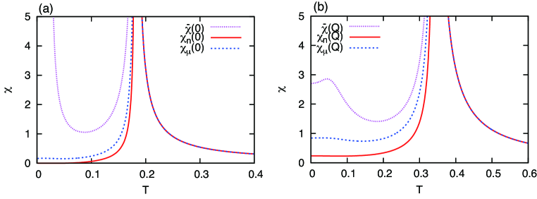
Figure 8: Longitudinal magnetic susceptibility as a function of temperature for a fixed chemical potential in the ferromagnetic (a) and antiferromagnetic (b) phase. The chemical potential is chosen as $\mu=-1.83$ in (a) which reproduces $n=0.2$ at $T=0.15$, and as $\mu=1.69$ in (b) where $n=1.1$ at $T=0.2$. The other parameters are $U=3$, $t^{\prime}=-0.45$ in (a) and $t^{\prime}=-0.2$ in (b). For $\chi_{n}$, the density is tuned at each temperature to reproduce the fixed chemical potential. The result of $\chi_{\mu}$ is correct in the whole temperature region.

References

- Izuyama et al. (1963) T. Izuyama, D. J. Kim, and R. Kubo, J. Phys. Soc. Jpn. 18, 1025 (1963).
- K. Ueda (1978) K. Ueda, J. Phys. Soc. Jpn. 44, 1533 (1978).
- Mukuda et al. (2012) H. Mukuda, S. Shimizu, A. Iyo, and Y. Kitaoka, J. Phys. Soc. Jpn. 81, 011008 (2012).
- Stewart (2011) G. R. Stewart, Rev. Mod. Phys. 83, 1589 (2011).
- C. Pfleiderer (2009) C. Pfleiderer, Rev. Mod. Phys. 81, 1551 (2009).
- H.-J. Lee and T. Takimoto (2012) H.-J. Lee and T. Takimoto, J. Phys. Soc. Jpn. 81, 104704 (2012).
- Rowe et al. (2012) W. Rowe, J. Knolle, I. Eremin, and P. J. Hirschfeld, Phys. Rev. B 86, 134513 (2012).
- Schrieffer et al. (1989) J. R. Schrieffer, X. G. Wen, and S. C. Zhang, Phys. Rev. B 39, 11 663 (1989).
- A. V. Chubukov and D. M. Frenkel (1992) A. V. Chubukov and D. M. Frenkel, Phys. Rev. B 46, 11884 (1992).
- A. P. Kampf (1994) A. P. Kampf, Phys. Rep. 249, 219 (1994).
- Knolle et al. (2010) J. Knolle, I. Eremin, A. V. Chubukov, and R. Moessner, Phys. Rev. B 81, 140506(R) (2010).
- Sokoloff (1969) J. B. Sokoloff, Phys. Rev. 185, 770 (1969).
- Igoshev et al. (2010) P. A. Igoshev, M. A. Timirgazin, A. A. Katanin, A. K. Arzhnikov, and V. Y. Irkhin, Phys. Rev. B 81, 094407 (2010).
- Moriya (1985) T. Moriya, Spin Fluctuations in Itinerant Electron magnetism (Springer, Berlin, 1985).
- (15) In the numerator of Eq. (52) in Ref. A. V. Chubukov and D. M. Frenkel, 1992, should be .