A critical study of the elastic properties and stability of Heusler compounds:
Phase change and tetragonal $X_{2}YZ$ compounds

Abstract

In the present work, the elastic constants and derived properties of tetragonal and cubic Heusler compounds were calculated using the high accuracy of the full-potential linearized augmented plane wave (FPLAPW). To find the criteria required for an accurate calculation, the consequences of increasing the numbers of $k$-points and plane waves on the convergence of the calculated elastic constants were explored. Once accurate elastic constants were calculated, elastic anisotropies, sound velocities, Debye temperatures, malleability, and other measurable physical properties were determined for the studied systems. The elastic properties suggested metallic bonding with intermediate malleability, between brittle and ductile, for the studied Heusler compounds. To address the effect of off-stoichiometry on the mechanical properties, the virtual crystal approximation (VCA) was used to calculate the elastic constants. The results indicated that an extreme correlation exists between the anisotropy ratio and the stoichiometry of the Heusler compounds, especially in the case of Ni₂MnGa.

Metastable, cubic Ni₂MnGa exibits a very high anisotropy ($\approx 28$) and hypothetical, cubic Rh₂FeSn violates the Born-Huang stability criteria in the $L2_{1}$ structure. The bulk moduli of the investigated tetragonal compounds do not vary much ($\approx 130\ldots 190$ GPa). The averaged values of the other elastic moduli are also rather similar, however, rather large differences are found for the elastic anisotropies of the compounds. These are reflected in very different spatial distributions of Young’s moduli when comparing the different compounds. The slowness surfaces of the compounds also differ considerably even though the average sound velocities are in the same order of magnitude ($3.2\ldots 3.6$ km/s). The results demonstrate the importance of the elastic properties not only for purely tetragonal Heusler compounds but also for phase change materials that exhibit magnetic shape memory or magnetocaloric effects.

I Introduction

Heusler-type intermetallic compounds $X_{2}YZ$ ($X,Y=$ transition metals, and $Z=$ main group elements) have become of particular interest due to their fascinating thermal, electrical, magnetic, and transport properties Graf et al. (2011). The Heusler compounds crystallize in a face-centered cubic (fcc) lattice. They are distinguished in two groups: regular or inverse Heusler compounds. Regular Heusler compounds belong to $Fm\overline{3}m$ (space group no. 225) symmetry, and inverse Heusler compounds belong to $F\overline{4}3m$ (space group no. 216). Both cubic phases may undergo a cubic–tetragonal phase transition, in which the regular Heusler compounds transform from $Fm\overline{3}m$ to the tetragonal $I4/mmm$ (no. 139), and the inverse Heusler compounds transform from $F\overline{4}3m$ to tetragonal $I\overline{4}m2$ (no. 119). Thus, the parent cubic and obtained tetragonally distorted phases obey a supergroup–subgroup relation.

Due to a simple feature of Heusler compounds, it is critically important to have an instrument for phase prediction. For example, cubic ferromagnetic Heusler compounds follow the Slater–Pauling rule for localized moment systems. Their magnetic moment $m$ depends simply on the valence electron concentration $n_{v}$ with $m=n_{v}-24$. Further, prospective candidates for superconductivity include certain Heusler compounds with 27 electrons that exhibit a saddle point at the $L$ point close to $E_{\rm F}$ in the band structure according to the van Hove scenario (Winterlik et al., 2009; van Hove, 1953). On the other hand, a high density of states at the Fermi level causes instability and a phase transition to lower symmetry forced by a band Jahn–Teller distortion Brown et al. (1999); Blum et al. (2011). This competition is one example that shows the importance of phase prediction in the Heusler compounds. However, both tetragonal and cubic phases have their own importance for industrial as well as fundamental research.

Tetragonally distorted Heusler compounds have attracted interest in the field of spintronics, in particular, for spin-torque applications, owing to their magnetic anisotropy in the perpendicular axes Winterlik et al. (2008); Krén and Kádár (1970); Wu et al. (2009, 2010). Therefore, the theoretical prediction of new materials with suitable design properties is active research in this field Gilleßen and Dronskowski (2010).

In fact, processing and designing new materials requires knowledge of physical properties, such as hardness, elastic constants, melting point, and ductility. The calculation of elastic constants is an efficient and fast tool used for elucidating physical properties as well as the mechanical stability and possible phase transitions of crystalline systems. Applied strains, such as shear or elongation, provide not only valuable information about the instability itself but also the directional dependence of instabilities in crystals. The directional dependence of instabilities becomes important when not only cubic–tetragonal but also cubic–hexagonal, tetragonal–hexagonal, and lower symmetry phase transitions are relevant, such as those observed in Mn₃Ga Winterlik et al. (2008); Krén and Kádár (1970). Unlike mechanical instability, the determination of elastic constants is essential for applications of magnetic shape memory alloys. The elastic constants also provide valuable information on the structural stability, anisotropic character, and chemical bonding of a system Gilman (2009, 2001); (1997) (Ed.). Moreover, other measurable properties can be estimated using the elastic constants, such as the velocity of sound, Debye temperature, melting point, and hardness. This information is an essential requirement for both industrial applications and fundamental research. For example, these properties are essential for studying superconductivity and heavy fermion systems in which a drastic change of elastic constants and related properties have been reported upon the phase transition Bruls et al. (1994); Ledbetter et al. (1989). The elastic properties are so important that Gilman Gilman (1960) concluded: “the most important properties of a crystal are its elastic constants”.

In the present study, some well-known tetragonal and cubic Heusler compounds are examined and compared with the available experimental and theoretical data Li et al. (2013, 2012); Luo et al. (2012); Li et al. (2011a, b); Hu et al. (2009a); Moya et al. (2006); Bungaro et al. (2003); de Jong et al. (2012). Starting from the cubic phase, cubic $L2_{1}$ Ni₂MnGa and Rh₂FeSn are considered for detailed studies. For the tetragonally distorted systems, Ni₂MnGa (in the non-modulated tetragonal ($c/a>1$) structure), Mn₂NiGa, Fe₂MnGa, and Mn₂FeGa Heusler compounds are examined. The intermetallics Mn${}_{2}Y$Ga ($Y=$ Fe, Ni) and $X_{2}$MnGa ($X=$ Fe, Ni) undergo tetragonal magneto–structural transitions that may result in half metallicity and magnetic shape memory or magnetocaloric effects. In the case of Ni₂MnGa, the composition dependence (chemical disorder effect) of the phase transition is studied using the virtual crystal approximation (VCA). Calculating the mechanical and elastic properties of off-stoichiometric compounds in the tetragonal phases elucidates phase transformations. Elastic constants and mechanical properties of some Rh-based Heusler compounds, reported by Suits Suits (1976), are calculated. The dependence of the elastic constants and the number of used $k$-points and plane waves (defined in full-potential linearized augmented plane wave (FPLAPW) by $R_{\rm MT}k_{\rm max}$, where $R_{\rm MT}$ is the muffin tin radius and $k_{\rm max}$ is the largest $k$ vector) are discussed in detail. The importance of using sufficiently large numbers of $k$-points and plane waves for a reliable estimation of the elastic properties is demonstrated.

The present work concentrates on the elastic properties of metastable cubic, tetragonal, and phase change materials that exhibit magnetic shape memory or magnetocaloric effects. The results for the famous series of half-metallic Co₂-based Heusler compounds that has a high impact on magnetoelectronics will be published elsewhere Wu et al. (2017).

II Methodology

II.1 Computational details

In this section, the basic equations for calculating the elastic constants are presented (for more details see Appendix A). The most easily determined quantity is the bulk modulus $B$, which provides the behavior of the crystal volume or lattice parameters under hydrostatic pressure. There are several ways to calculate the bulk modulus from the energy–volume $E_{\rm tot}(V)$ relation (see References Ziambaras and Schröder, 2003; Birch, 1947; Murnaghan, 1944). In the present work, the bulk modulus $B$ is determined by fitting the total energy calculations to the Birch–Murnaghan equation of state Birch (1947); Murnaghan (1944). According to this model, the dependence of the energy on the change in the crystal volume $V$ under hydrostatic pressure $p$ is given by

$$E=E_{0}+\frac{9}{16}\frac{BV_{0}}{14703.6}\left[(6-4v^{2})\eta^{2}+B^{\prime}\eta^{3}\right],$$ (1)

where $B^{\prime}=dB/dp$ is the pressure derivative of the bulk modulus and $\eta=v^{2}-1$, with the ratio $v=(V_{0}/V)^{1/3}$ of the actual volume $V$ under pressure to the relaxed volume $V_{0}$ at the lowest total energy $E_{0}$ (see Reference Wallace, 1972). The related pressure is given by

$$p=\frac{3}{2}B(v^{7}-v^{5})\left[1+\frac{3}{4}(B^{\prime}-4)\eta\right].$$ (2)

For tetragonal crystals, the dependence of the bulk modulus $B$ on the elastic stiffness is given by

$$B=\frac{1}{9}(2c_{11}+2c_{12}+4c_{13}+c_{33}).$$ (3)

In the case of cubic crystals, $c_{12}=c_{13}$, $c_{11}=c_{33}$, and $c_{44}=c_{66}$ (see also Appendix A). Therefore, the equations of the elastic constants for cubic systems are easily obtained from the tetragonal equations.

The remaining elastic properties are determined by applying different types of strain ($e_{i}$) to the tetragonal lattice and by applying proper relations between the total energy and the strain components. The energy $E(e_{i})$ of the strained lattice is calculated using Hooke’s law (see equation (10)). According to Wallace Wallace (1972), if the strains $e_{i}$ are small, the change of the energy is given by

$$\frac{\Delta E}{V_{0}}=\sum\Delta_{i}e_{i}+\frac{1}{2}\sum\sum c_{i,j}e_{i}e_{j}.$$ (4)

Here, $\Delta E=E(e_{i})-E_{0}$ with equilibrium energy $E_{0}$ at volume $V_{0}$ without strain. The linear terms vanish at equilibrium or if the strain causes no change in the volume of the crystal. The elastic constants $c_{i,j}$ are obtained from the second-order terms and are calculated from the second derivatives of the energy with respect to the strains:

$$c_{i,j}=2\left.\frac{\partial^{2}E}{\partial e_{i}\partial e_{j}}\right|_{V=V_{0}}$$ (5)

The second derivative relation of elastic constants ($c_{ij}$) with total energy highlights the importance of an accurate calculation of the total energy. Therefore, the choice of the density functional theory solver in the calculation of elastic constants and related properties is significant.

For cubic crystals, three independent elastic constants need two strains for calculations, while in tetragonal systems (space group Nos. 89–142), six independent elastic constants need five different strains. In fact, there are numerous ways to apply the six different strains and their combinations to the crystal. The necessary side condition of equation (5) is that the volume must be conserved when applying the strain. Therefore, the use of linear strain components ($e_{i}=\delta$ in all possible cases and combinations in the strain matrix of equation 9 of Appendix A) would lead to large uncertainties because they are not always volume conservative, or they make the use of additional derivatives necessary (for example, $\frac{\partial E}{\partial V}$, $\frac{\partial V}{\partial e_{i}}$, and higher orders).

Table 1: Strain table for calculation of the elastic constants in tetragonal systems.
Note that only types (1) to (5) are volume conservative. Only components with $e_{i}\neq 0$ are given. Type (0) corresponds to calculation of the bulk modulus.

Type		Strain			$\Delta E/V_{0}$
(0)	isotropic	$e_{1}=\delta$	$e_{2}=\delta$	$e_{3}=\delta$	(see bulk modulus)
(1)	monoclinic	$e_{1}=\delta^{2}/(1-\delta^{2})$	$e_{4}=\delta$		2$c_{44}\delta^{2}+O(\delta^{4})$
(2)	triclinic	$e_{3}=\delta^{2}/(1-\delta^{2})$	$e_{6}=\delta$		2$c_{66}\delta^{2}+O(\delta^{4})$
(3)	orthorhombic	$e_{1}=\delta$	$e_{2}=-\delta$	$e_{3}=\delta^{2}/(1-\delta^{2})$	$(c_{11}-c_{12})\delta^{2}+O(\delta^{4})$
(4)	orthorhombic	$e_{1}=\delta$	$e_{2}=\delta^{2}/(1-\delta^{2})$	$e_{3}=-\delta$	$(c_{11}-2c_{13}+c_{33})\delta^{2}/2+O(\delta^{4})$
(5)	tetragonal	$e_{1}=\delta$	$e_{2}=\delta$	$e_{3}=-\delta(2+\delta)/(1+\delta)^{2}$	$(c_{11}+c_{12}+2c_{33}-4c_{13})\delta^{2}/2+O(\delta^{4})$
(6)	tetragonal	$e_{3}=\delta$			$c_{33}\delta^{2}/2$

Table 1 and Figure 1 summarize the applied strains that are used to determine the elastic constants in the present work. The applied strains are the same as those reported by Kart et al Kart et al. (2008). The isotropic strain (0) is not used directly for the calculation of the elastic constants, as it gives the same information as discussed for the bulk modulus $B$ (see discussion above). The five strain types (Equations (1)–(5) in Table 1) are chosen to be volume conservative. The last strain type does not conserve the volume, but it keeps the same symmetry as the crystal and thus can be calculated from the energy versus $c/a$ relation Kart et al. (2008), where $c/a$ is the ratio of the two independent lattice parameters of the tetragonal crystals.

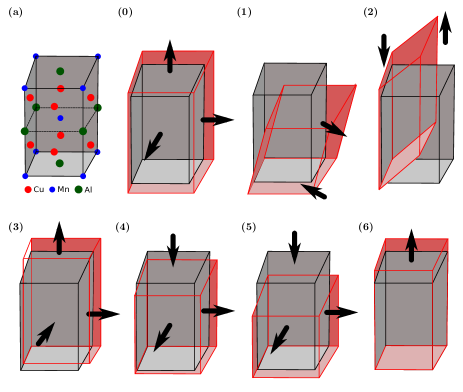
Figure 1: (Online color) Strain types for calculation of the elastic constants in tetragonal systems.
(a) shows the tetragonal Heusler structure with $I\>4/mmmm$ symmetry. (0)–(6) show the strain types and resulting distortions according to Table 1.

In the present work, six distortions of each type in the range of $-3\%\leq\delta\leq+3\%$ were applied to the relaxed structure with $V_{0}$ from the structural optimization using the Birch–Murnaghan equation of state. For tetragonal systems, the energy $E(\delta)$ versus applied strain curves were fitted to a fourth-order polynomial $E(\delta)=E_{0}+a_{2}\delta^{2}+a_{3}\delta^{3}+a_{4}\delta^{4}$.

Here, an additional method of verifying the convergence as well as the accuracy of the results is introduced. In principle, it is sufficient to use either Equation (4) or (5) of Table 1 to calculate all six elastic constants. However, the elastic constants and all related properties are calculated with both equations to ensure that they provide the same results. This happens, indeed, only if the results are well converged (see also Section III.1). The system is overdetermined by using both types of strains; however, in this way, the accuracy of the calculated quantities can be estimated. In fact, the values reported here have an error below 0.5%. The combination of different strains as well as different types of equations of state allow determination of the uncertainty of the calculated results, which is expected for a reliable computer experiment.

II.2 Electronic structure calculations

The ab-initio electronic structure calculations were performed using the Wien2k code Blaha et al. (2001). The all-electron full-potential method, FLAPW, with an unbiased basis covers all elements of the periodic table with any spin configuration. This feature is essential for Heusler compounds because they may contain diverse types of atoms, including lanthanide and actinide atoms, together with exotic magnetic ordering. The accuracy of this method makes it suitable for the studied systems. For example, Co₂TiAl fails with spherical potentials or full symmetry potentials together with bare exchange–correlation functionals neglecting gradient corrections Graf et al. (2009); Ishida et al. (1982); Mohn et al. (1995). Since elastic constants are calculated from the second derivatives of the total energy, an accurate calculation of total energy is extremely important.

The exchange–correlation functional was taken in the generalized gradient approximation of Perdev, Burke, and Enzerhoff (GGA-PBE) Perdew et al. (1997, 1996). The number of plane waves was restricted by $R_{\rm MT}k_{\rm max}=9$, and the number of $k$-points was set to 8000 $k$-points in the full Brillouin zone. As discussed in Section III.1, these criteria ensure the convergence of the calculated elastic properties for the investigated systems.

The lattice parameters were optimized before calculating the elastic constants. The results of the structural optimizations are summarized in Table 2 along with some previously reported experimental and theoretical values. Here, the $c/a$ ratio was obtained by a full optimization of the Heusler compounds in tetragonal space groups 119 or 139. In other words, to find the energy minimum, not only the $c/a$ ratio changed (the elongation of $c$)  Kart and Çağ ın (2010); Kart et al. (2008) (see also Figure 2) but also the volume of the structures was relaxed. The assignment of lattice parameters should be performed carefully since the optimization was performed in the tetragonal symmetry. When reducing the cubic $fcc$ cell to a tetragonal $fct$ cell, the cubic lattice parameter $a=a_{c}$ becomes $c$, and the tetragonal parameter $a=a_{t}$ becomes $a_{c}/sqrt(2)$. To better understand the distortion of the cubic Heusler structure to the tetragonal Heusler structure, the distortion parameter $\varepsilon$ is defined by

$$\varepsilon=\frac{c}{a_{t}}\frac{1}{\sqrt{2}}-1,$$ (6)

where $a_{t}$ is the tetragonal $a$ parameter. At $\varepsilon=0$, the structure is cubic; at $\varepsilon<0$, the cubic cell is compressed; and at $\varepsilon>0$, the cubic cell is elongated along one of the principal axes.

Table 2: Results of the structural optimization. Lattice parameters $a$ and $c$ are given in Å, $\varepsilon$ is dimensionless, and total magnetic moments $m$ are in $\mu_{\rm B}$. All structures are fully optimized ($V$, $c/a$, magnetic state) for the given symmetries. Column sym gives the number of the corresponding space group, and cubic and tetragonal structures are assigned by the Pearson symbols $cF16$ and $tI4$, respectively. Experimental values are given for comparison. Note that the cubic variant of Rh₂FeSn is only hypothetical.

Compound	sym	$a_{c}$, $c$	$a_{t}$	$\varepsilon$	$m_{\rm tot}$
Mn2NiGa	$tI4$ 119	6.91	3.78	0.293	1.0
Ni2MnGa	$tI4$ 139	6.80	3.78	0.272	4.0
Exp.		6.44	3.90	0.168	4.09
Ni2MnGa	$cF16$ 225	5.81		0	4.1
Exp.		5.82		0	4.17
Mn2FeGa	$tI4$ 119	7.30	3.68	0.403	0.77
Fe2MnGa	$tI4$ 139	7.31	3.62	0.428	0.13
Rh2CrSn	$tI4$ 139	7.33	4.08	0.270	2.40
Exp.		7.16	4.09	0.238
Rh2FeSn	$tI4$ 139	7.12	4.13	0.219	3.92
Exp.		6.91	4.15	0.177	3.70
Rh2FeSn	$cF16$ 225	6.25		0	3.54
Rh2CoSn	$tI4$ 139	7.22	4.05	0.261	2.25
Exp.		6.90	4.14	0.179	2.44

The magnetic state was verified using different settings of the initial magnetization: ferromagnetic (all initial spins parallel) or ferrimagnetic (initial spins partially antiparallel). From the studied systems, all Mn₂YZ compounds exhibit ferrimagnetic order in which one Mn has majority and the other Mn has minority orientation. For all other compounds, the ferromagnetic ground state has the lowest total energy.

III Results

Prior to discussing the tetragonal Heusler compounds, the elastic constants of the unstable and metastable cubic systems are discussed. Here, Ni₂MnGa with $L2_{1}$ structure is selected as a metastable system. This compound is one of the most investigated materials owing to its shape memory behavior and its potential applications in actuator devices. In fact, in Section III.1, only the cubic phase is addressed, and the tetragonal phase of Ni₂MnGa is discussed in Section III.2. Moreover, Ni₂MnGa was used as an example case to study the significance of increasing the number of $k$-points and plane waves and their relations to the convergence of the elastic constants. In the second part of this section, the tetragonal phase of Heusler compounds are discussed. The elastic constants together with the corresponding measurable properties for selected tetragonal Heusler compounds are investigated. The role of the stoichiometry on the phase transition of Ni₂MnGa is also explored.

III.1 Elastic constants and metastability in cubic and tetragonal compounds.

Stoichiometric Ni₂MnGa undergoes a structural phase transition from the austenite into the martensite phase Tsunegi et al. (2008). Depending mostly on the composition, the martensite structure is characterized by the tetragonal $5M$ modulated structure with $c/a\approx 0.94$, the orthorhombic $7M$ structure with $c/a\approx 0.9$, and the non-modulated tetragonal structure with $c/a\approx 1.2$ [Kart and Çağ ın, 2010]. Figure 2 shows the appearance of different stable and metastable phases with varying $c/a$ elongation. To focus on the cubic phase, Figure 2(b) shows only the small range of strains with $c/a<1$ that cover the cubic phase. The deepest energy minimum is located at a strain of about $\varepsilon=0.27$, corresponding to $c/a\approx 1.26$ (non-modulated phase). A shallow minimum (see Figure 2(b)) appears at a strain of about -0.05 ($c/a\approx 0.94$, 5M phase). The elastic constants of the structure with $c/a>1$ will be discussed in Section III.2.

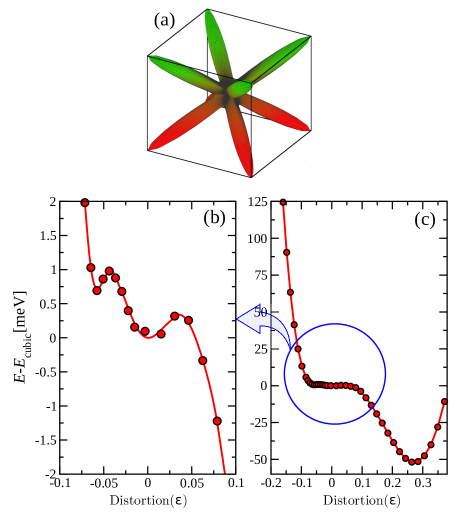
Figure 2: (Online color) (a) The calculated spatial distributions of the rigidity modulus $G(\hat{r})$ of Ni₂MnGa. (b, c) The total energy as a function of tetragonal strain along the $c$-axis at constant volume. Panel (b) focuses on the 5M modulated phase with $c/a\approx 0.9$

As shown in Figure 2(c), the metastable cubic phase exists only under an infinitesimal strain and exhibits a very low energy modulation. The optimized lattice constant of cubic Ni₂MnGa with the $L2_{1}$ structure is 5.81 Å, in excellent agreement with the experimental value of 5.82 Å [Webster et al., 1984]. This phase is only stable within $\pm 1$ meV energy changes, which confines the lattice distortion to $<\pm 1$%. This distortion relates to the tetragonal distortion, providing the $c_{11}-c_{12}$ combination of elastic constants. To observe such a non-trivial change in energy and to have a smooth dependence on strain, the results need to be precisely converged with very high precision. This does not imply, however, that the results do not need to be converged for a wide energy window with a deep minimum. As an example, the importance of converged results is demonstrated in Figure 3. The $c_{44}$ shear modulus is stable for a lattice distortion of about $\pm 3$% and an energy change of more than $\pm 30$ meV. In this case, the rough calculation provides a smooth curve, but the calculated elastic constants significantly deviate from the converged results. The convergence of the results have the same importance for the calculation of the bulk modulus ($B$) (see Figure 3(c,d)).

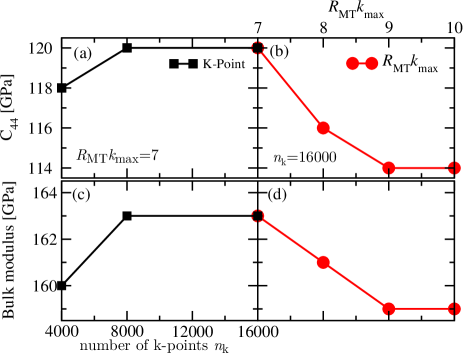
Figure 3: (Online color) Convergence of elastic properties.
The shear modulus $c_{44}$ and bulk modulus ($B$) as a function of $R_{\rm MT}k_{\rm max}$ and the number of $k$-points. The right side panels (a,c) show the increment of $B$ and $c_{44}$ as a function of the $k$-points with $R_{\rm MT}k_{\rm max}$=7. Using the converged $k$-points (16000 or 8000), in the left side panels (b,d), these values decrease with increasing $R_{\rm MT}k_{\rm max}$. Therefore, the minimum number of $k$-points and value of $R_{\rm MT}k_{\rm max}$ are 8000 and 9, respectively.

Figure 3 shows the convergence of $c_{44}$ and $B$ with respect to $R_{\rm MT}k_{\rm max}$ and number of $k$-points. As shown in (a,c) for constant $R_{\rm MT}k_{\rm max}=7$, increasing the number of $k$-points increases the $c_{44}$ and $B$ values. These results converge at 8000 $k$-points. In contrast, increasing $R_{\rm MT}k_{\rm max}$ decreases $c_{44}$ and $B$. Note that a similar result could be obtained at a more relaxed criterion, for example at 2000 $k$-points and $R_{\rm MT}k_{\rm max}=7$, due to error cancellations. Therefore, $R_{\rm MT}k_{\rm max}=9$ and 8000 $k$-points are the minimum criteria to converge the results for the systems studied in this work.

Table 3: Elastic properties of metastable Ni₂MnGa and hypothetical Rh₂FeSn with $L2_{1}$ structure.
The calculated elastic parameters $c_{ij}$, $c^{\prime}$, and $B$ are given in GPa, and the cubic elastic anisotropy $A_{e}=\frac{2c_{44}}{c_{11}-c_{12}}$ is dimensionless and corresponds to the tetragonal $A_{001}$.

Compounds	$c_{11}$	$c_{12}$	$c_{44}$	$c^{\prime}$	$B$	$A_{e}$
Ni2MnGa	164	156	115	4.1	159	28.02
Exp.	152	143	103	4.5	146
Other calc.	163	152	107	5.5	156
Rh2FeSn	124	206	84.3	-82	179	$<0$

The calculated elastic constants of Ni₂MnGa with $L2_{1}$ structure are given in Table 3. The calculated results show a reasonable agreement with the experimental results and coincide with previously reported theoretical results Kart et al. (2008); Kart and Çağ ın (2010). Note, however, that good agreement with the experiment results does not guarantee the accuracy of the calculations. First, the experiments were performed at 300 K for Ni₂MnGa in the $L2_{1}$ phase, and off-stoichiometry has a significant effect on the measured elastic constants Hu et al. (2009b). Moreover, the employed experimental method may result in different measured elastic constants Worgull et al. (1996). As an example, the $c_{44}$ value deviates by about 60 GPa based on the experimental method. In general, the measured elastic constants are inversely related to temperature Ledbetter (2006). Hence, a higher value should be expected for the calculations. Fortunately, $c^{\prime}$, which is a difference between two constants ($c_{11}$ and $c_{12}$), is argued to be less dependent on temperature Ledbetter (2006). In fact, the calculated $c^{\prime}=4.5$ GPa exhibits a better agreement with the experiment (4.1 GPa) than previously reported values Kart et al. (2008); Kart and Çağ ın (2010).

In addition, $c_{12}$ and $c_{11}$ do not have any physical basis; in other words, no phonon mode directly corresponds to these constants. Mixing with other stiffness ($c_{ij}$), however, results in a meaningful combination. For example, the tetragonal shear modulus $c^{\prime}=(c_{11}-c_{12})/2$ corresponds to cubic–tetragonal distortion. Moreover, it is well established that $c^{\prime}$ – associated with slow transverse acoustic waves Worgull et al. (1996) – plays an important role in the occurrence of structural transformations. Another important quantity is the Cauchy pressure $c_{p}=c_{12}-c_{44}$. A negative value of $c_{p}$ ($c_{12}<c_{14}$) may indicate covalent bonds, where the angular dependence of the inter-atomic forces becomes important.

Furthermore, detailed analysis of elastic constants sheds light on the stability and phase transition in Heusler compounds. Cubic Ni₂MnGa with soft $c^{\prime}$ is on the border of the phase transition. With the similar interpenetration (see Appendix B), the large elastic anisotropy $A_{e}$ of Ni₂MnGa ($A_{e}$=28) hints on its tendency to deviate from the cubic structure. Anisotropy is another indicator for the instability of cubic structures. The elastic anisotropy of crystals is also an important parameter for engineering since it correlates to the possibility of micro-cracks in materials. Unlike the mechanical properties, anisotropy shows the tendency of a system toward phase transitions as it inversely relates to the $c^{\prime}$ parameter. In fact, an illustrative way to show the anisotropy is to visualize the rigidity modulus $G(\hat{r})$ or Young’s modulus $E(\hat{r})$. Figure 2(a) shows that the rigidity modulus is largest in the $\left<111\right>$-type direction that is along the tetragonal axes. Such a significant deviation from spherical shape indicates that the moduli of Ni₂MnGa exhibit a large degree of anisotropy. In principle, when $c_{11}-c_{12}\rightarrow~{}0$, the rigidity distribution exhibits a stronger directional dependency, as shown for Ni₂MnGa in Figure 2(a).

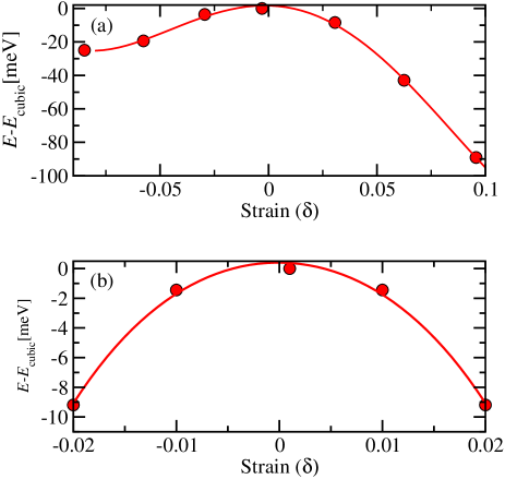
Figure 4: (Online color) Energy–strain relation for hypothetical Rh₂FeSn with $L2_{1}$ structure.
Displayed are the calculated total energies as function of (a) tetragonal (symmetry No. 139) and (b) orthorhombic (symmetry No. 69) strains.

In the next step, a compound that is not stable in the cubic structure was examined for comparison. In the case of Rh₂FeSn shown in Figure 4, the cubic structure exhibits a maximum of the total energy, and any tetragonal distortion will lead to a different stable structure. Based on Figure 4, the appearance of energy minima are expected for two different tetragonally distorted systems with $c/a>1$ and $c/a<1$. Larger distortions show that $c/a>1$ is the stable phase, while $c/a<1$ is a metastable phase. Previous works only reported the structure with $\varepsilon>0$ Suits (1976); Dhar et al. (1980). However, the calculated elastic constants also supported the instability of the cubic phase from negative values of tetragonal shear modulus $c^{\prime}$ and anisotropy $A_{\rm e}$. The metastable structure with $\varepsilon<0$ appears when expanding the in-plane lattice parameter $a$ while keeping $c$ at the cubic lattice parameter. Such a situation may be artificially initialized by epitaxial or pseudomorphic thin film growth on a substrate with an appropriate lattice parameter. Similar metastable situations may exist in many other tetragonal Heusler compounds and will open the field of lattice parameter engineering to enlarge the number of properties on demand.

III.2 Tetragonal Heusler compounds

The tetragonal Heusler compounds studied in this work along with their elastic constants are summarized in Tables 4 and 5. The Heusler intermetallics Mn${}_{2}Y$Ga ($Y=$Fe, Ni) and $X_{2}$MnGa ($X=$Fe, Ni) undergo tetragonal magneto-structural transitions that result in half-metallicity, magnetic shape memory, or magneto-electric effects. In this section, the off-stoichiometric compositions are briefly discussed, and then, the elastic constants and related properties of the Heusler compounds are analyzed. Calculating the elastic properties of the tetragonal phases illuminates the structural transformations, chemical bonding, and mechanical stability of these intermetallic compounds for applications. Likewise, the elastic properties of Rh-based Heusler compounds synthesized by Suits Suits (1976) are calculated. Although Ni₂MnGa has been widely studied experimentally at different phases, there is no experimental measurement of the elastic modulus of the non-modulated tetragonal phase, and only theoretical works on this phase have already been reported Kart and Çağ ın (2010); Kart et al. (2008).

Table 4: Elastic properties of selected tetragonal Heusler compounds. The different moduli ($B,G,E$) and elastic constants $c_{ij}$ are given in GPa, the corresponding elastic compliances $s_{ij}$ are in (TPa)^-1. The anisotropies ($A_{\rm B}$ , $A_{100}$, $A_{001}$), Phug’s ratio $k$, and Poisson’s ratio $\nu$ are dimensionless. The compressibility $\kappa$ is in GPa^-1. For Ni₂MnGa, results taken from Reference Kart and Çağ ın, 2010 are given in brackets ().

	Mn2NiGa			Ni2MnGa			Mn2FeGa	Fe2MnGa	Rh2CrSn	Rh2FeSn	Rh2CoSn
		normal	25.1Mn	30.9Ga	28.1Ni	27.9Ni
$B_{\rm V}$	134.9	159.2 (158)	161.8	158.9	158.0	161.3	141.2	154.7	176.6	178.8	187.8
$B_{\rm R}$	126.5	159.2 (157.8)	161.7	131.6	157.5	155.1	134.6	154.3	161.6	176.5	185.8
$B$	130.7	159.2 (157.9)	161.8	145.2	157.8	158.2	137.9	154.5	169.1	177.7	186.8
$G_{\rm V}$	109.3	95.9 (73.8)	95.9	96.0	93.7	95.1	106.6	116.2	108.3	86.2	101.5
$G_{\rm R}$	80.5	66.3 (53.8)	66.6	57.2	62.5	50.3	37.9	56.1	85.2	74.6	76.5
$G$	94.8	81.1 (63.6)	81.2	76.6	78.1	72.7	72.3	86.2	96.7	80.4	89.0
$E$	229.2	208 (208)	208.8	195.4	201.1	189.1	184.6	218.0	243.7	209.6	230.4
$c^{\prime}$	67	60	62	60	58	67	12	21	73	70	67
$c_{11}$	194	227 (252)	235	196	229	222	181	195	234	252	257
$c_{12}$	60	108 (74)	112	77	113	88	157	154	88	113	123
$c_{13}$	118	140 (144)	142	157	139	156	110	122	160	153	168
$c_{33}$	232	199 (194)	196	255	184	208	151	205	300	265	258
$c_{44}$	163	148 (100)	145	151	143	150	167	177	154	124	154
$c_{66}$	110	95 (55)	100	93	99	91	155	162	112	66	94
$s_{11}$	7.45	7.80 (7.26)	7.61	10.43	8.05	10.21	23.26	14.76	6.72	6.25	6.82
$s_{12}$	0.02	-0.58 (1.65)	-0.57	2.05	-0.53	2.76	-17.60	-9.83	-0.14	-0.94	-0.66
$s_{13}$	-3.80	-5.09 (-6.61	-5.09	-7.69	-5.66	-9.69	-4.13	-2.95	-3.51	-3.06	-3.99
$s_{33}$	8.17	12.21 (15.0)	12.47	13.40	13.97	19.29	12.66	8.41	7.06	7.30	9.05
$s_{44}$	6.11	6.80 (10.0)	6.89	6.63	7.01	6.67	6.00	5.66	6.47	8.06	6.47
$s_{66}$	9.01	10.51 (18.2)	10.04	10.74	10.10	10.98	6.46	6.16	8.89	15.05	10.64
$A_{\rm B}$	0.15	0.93	1.17	-0.41	1.42	-0.03	2.89	1.27	0.015	0.52	0.49
$A_{100}$	3.44	4.04	3.94	4.39	4.20	5.04	5.97	4.57	2.88	2.35	3.44
$A_{001}$	1.64	1.59	1.63	1.56	1.70	1.36	12.64	7.98	1.54	0.95	1.41
$k$	1.38	1.96 (2.48)	1.99	1.90	2.02	2.18	1.91	1.79	1.75	2.20	2.09
$\nu$	0.21	0.282 (0.322)	0.28	0.28	0.29	0.30	0.28	0.26	0.26	0.30	0.29
$\kappa$	0.0079	0.0063	0.0062	0.0076	0.0063	0.0064	0.0079	0.0065	0.0062	0.0056	0.0054

As shown in Table 4, in the case of Ni₂MnGa, the results show a qualitative agreement with the previous theoretical report (values in brackets). However, a quantitative comparison of the results reveals some significant deviations. These differences can be traced back to the calculation method and the method of performing structural optimization. To address this problem, the cubic phase is briefly considered. In the cubic phase, the present as well as other calculations are performed for the same lattice parameters using different calculation schemes. Here, the results of FPLAPW calculations are slightly larger than those of projected augmented wave (PAW) calculations, and the deviations range from 1% for $c_{11}$ up to 7% for $c_{44}$. These small differences are expected because of the selected methods and convergence criteria. In contrast, in the case of the tetragonal system (see Table 4), the deviations between calculations range up to 30%, such as the case of $c_{44}$ and $c_{66}$. Indeed, the different calculation methods should not lead to such a large discrepancy (if all factors are set carefully), and these observed differences mainly arise from the underlying structural optimization. Here, all initial tetragonal structures are fully optimized at their relevant symmetries ($I4/mmm$ or $I\overline{4}m2$), and thus, they differ from the simply elongated cubic structures (see also Section II.2 for more details about the calculations).

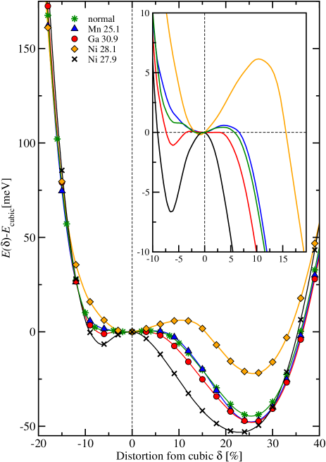
Figure 5: (Online color) The energy change along $c/a$ is plotted for the non-stoichiometry composition of Ni₂MnGa. The energy landscape (here, along the c-axis) is extremely sensitive to the stoichiometric composition, in particular, the Ni component.

The elastic constants of all studied tetragonal Heusler compounds follow the inequality $B>c_{44}>G>c^{\prime}>0$, so that the tetragonal shear modulus $c^{\prime}$ is the main constraint on the stability and properties. Pugh’s and Poisson’s ratio (see Appendix A) supply valuable information about the malleability and the type of bonding in crystals. Small values of Pugh’s ratio indicate low malleability of crystals Pugh (1954), meaning they are brittle. Pugh’s ratio indicates the type of bonding, namely covalent or metallic bonding, because changes in the angle of a covalent bond require more energy than stretching– stressing the bond, meaning $G$ becomes larger compared to $B$; this leads to smaller values of $k$. On the other hand, Poisson’s ratio for covalent bonding is about $\nu=0.1$ and increases for ionic crystals up to $\nu=0.25$. For instance, Pugh’s and Poisson’s ratios of strong covalent compounds such as diamond are assumed to be $k=0.83$ and $\nu=0.069$, respectively, while in the strongly ionic KCl, Pugh’s and Poisson’s ratios are $k=1.19$ and $\nu=0.27$, respectively McSkimin and Bond (1957); Lazarus (1949). Despite having different types of bonding, both KCl and diamond are brittle. On the other hand, strongly malleable gold exhibits ratios of $k=6.14$ and $\nu=0.42$ Niu et al. (2012); Pugh (1954), and gold is the most ductile metallic element. According to Christensen Christensen (2013), the critical value for the ductile–brittle transition appears at a Pugh’s ratio of

$$k_{B/D}=\frac{2}{3}\frac{1}{(1-\sqrt{1/2})}\approx 2.3,$$ (7)

which corresponds to a critical Poisson’s ratio of $\nu_{B/D}=(3\sqrt{2}-1)^{-1}\approx 0.31$. This criterion will be analyzed in more detail in a forthcoming work on cubic Heusler compounds Wu et al. (2017). Based on the calculated elastic constants, the studied tetragonal compounds exhibit Pugh’s ratios between 1.38 and 2.2 and Poisson’s ratios between 0.21 and 0.3, indicating that they have an intermediate behavior between ductile- and brittle- type behavior. The values of $k$ and $\nu$ indicate the covalent or metallic character of these systems. More details about the bonding type may be found from a Bader analysis of the charge densities Bader (1990); Otero-de-la Roza et al. (2009, 2014).

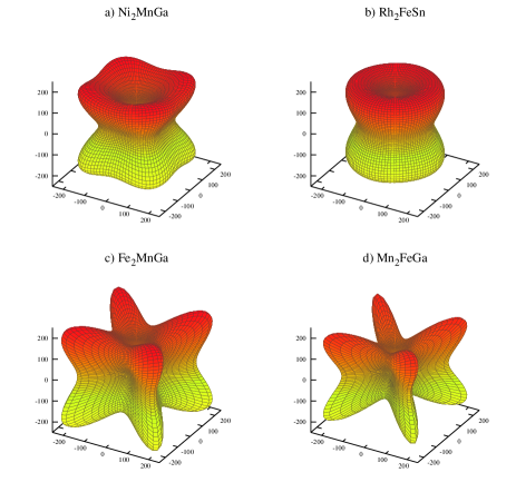
Figure 6: (Online color) Calculated spatial distribution of Young’s moduli $E(\hat{r})$ of some Mn- and Rh-based Heusler compounds. The change from the round shape of Rh₂FeSn to the sharply elongated shape in Mn₂FeGa indicates an increase of the elastic anisotropy (see also Table 4).

The shear anisotropy factor $A_{\rm e}$ provides a measure of the degree of anisotropy of the bonds between atoms in different planes. Tetragonal systems are described by two different shear anisotropic factors $A_{001}$ and $A_{100}$ (or equivalent $A_{010}$). Young’s moduli of some of the studied Heusler compounds are shown in Figure 6. The shear anisotropy for {100} planes is considerably higher compared to {001} planes for Mn₂NiGa and Rh₂FeSn. This behavior is similar for Mn₂FeGa and other Rh₂-based compounds, as shown in Table 4. In contrast, in the case of Fe₂MnGa and Mn₂FeGa, the anisotropy for {001} is higher than that for {100}. Moreover, Rh₂FeSn has an interesting distribution of Young’s modulus: it is isotropic in the square x-y planes of the tetragonal structure, arising from the value of $A_{001}=0.95$, which is close to unity.

III.3 Virtual Crystal Approximation

One interesting feature of Heusler compounds, including Ni₂MnGa, is their sensitivity to stoichiometric compositions. An infinitesimal deviation may lead to a phase transition or to changes in the electronic structure properties. Here, VCA was applied to explore off-stoichiometric systems. This approximation is valid for small changes of components with nearly the same radius, which holds for the considered systems. Moreover, VCA is only valid for neighboring elements and for small differences in the number of valence electrons ($\Delta e^{-}<0.1$).

In VCA, the atom ${}^{Z}A$ with charge $Z$ is replaced by atom ${}^{Z^{\prime}}A$ with the virtual charge $Z^{\prime}=Z\pm\epsilon$ to reflect that the average charge deviates from the original value at a certain position. In Ni₂MnGa, if the site where ²⁸Ni resides is partially occupied by ²⁵Mn, the charge at that site will be lower; accordingly, the charge will be higher when ³⁰Ga occupies the same site. In parallel to the change in the nuclear charge, the number of electrons in the primitive cell changes to remain neutral. Thus, for ^28±ϵNi₂²⁵Mn³¹Ga, the number of valence electrons will be $n_{v}=30\pm 2\epsilon$ in the primitive cell, whereas the number of core plus semi-core electrons stays fixed at 72. The following cases are used in the present work:

• ^30.9Ga $=>$ Ni or Mn at Ga site,

• ^25.1Mn $=>$ Ni or Ga at Mn site,

• ^27.9Ni $=>$ Mn at Ni site, and

• ^28.1Ni $=>$ Ga at Ni site.

All elongated structures of off-stoichiometric Ni₂MnGa have been fully optimized within the VCA approximation. As shown in Figure 5, a small change in the number of electrons at the Ni site has the most drastic effect on the energy landscape. The largest difference appears between Ga-rich (^28.1Ni) and Ni-poor (^27.9Ni) compounds. Increasing Ni at Ga and Mn sites lowers the energy minimum at $c/a>1$ compared to the stoichiometric compound. Conversely, increasing Ga at the Ni site increases the energy of $c/a>1$ with respect to the stoichiometric compound. These results are in agreement with previously reported calculations Zayak and Entel (2004). Differences in the $E(\delta)$ dependence are more pronounced when the distorted structure is far from the initial structure. In the next step, the elastic constants of the off-stoichiometric Ni₂MnGa were calculated using VCA for the tetragonal distorted structures with $c/a>1$ at the lowest total energy (see Figure 5).

Table 4 summarizes the results of the elastic constant calculations for stoichiometric and off-stoichiometric Ni₂MnGa. An extreme effect of the off-stoichiometry is reflected in the anisotropy ratio ($A_{B}$). As shown in Table 4, the ^27.9Ni and ^30.9Ga compounds exhibit negative anisotropies of -0.02 and -0.4, respectively. In fact, the negative anisotropy highlights the extreme instability of these systems. In particular, ^30.9Ga has a large negative value. The results explain why ^30.9Ga (Ga-poor) and ^27.9Ni (Mn-rich) Ni₂MnGa synthesis is difficult. Moreover, the ^28.1Ni (Ga-rich) and ^25.1Mn (Mn-poor) compounds have large anisotropies, which are twice the value of the stoichiometric anisotropies. The large value also explains the tendency of phase transitions in these materials. Therefore, off-stoichiometric Ni₂MnGa – nearly all synthesized samples are slightly off-stoichiometric – is expected to have pronounced phase transitions depending on the composition Jiang et al. (2003). Thus, deficiency of valence electrons at the Mn or Ga sites in these systems leads to a negative anisotropy ratio and thus structural instability. Among the elastic constants, $c_{11}$ and $c_{22}$ are more strongly influenced when the composition changes compared to $c_{66}$ and $c_{44}$, which remain nearly constant. Therefore, a small excess of each of the elements (small change of the valence electron concentration in the vicinity of that site) will not change the shear in the [100] direction. However, the asymmetries $A_{B}$ and $A_{100}$ significantly change compared to $A_{001}$, reflecting a change of the in-plane chemical bonding. Here, Ni₂MnGa is used as an example of the sensitivity of Heusler compounds on their stoichiometry. Disorder-induced phase transitions have been reported for other Heusler compounds such as iron-based compounds Gasi et al. (2013).

III.4 Derived properties of tetragonal Heusler compounds

Finally, some physical properties and material parameters of the compounds are derived from the calculated elastic properties. The velocity of sound is an important quantity. Its averaged values can be directly determined from the calculated elastic constants. In experiments, on the other hand, the sound velocities can be used to measure elastic constants. Therefore, the sound velocities $v$ are nearly synonymous with the elastic stiffness constants $c$. Further, sound velocities have been used to study various solid-state properties and processes Ledbetter (2006). Therefore, having the sound velocities predicted by calculations in advance could be quite important for experimental measurements. Usually, the directionally dependent acoustic properties are analyzed in terms of the slowness that is the inverse of the phase velocity. The group velocities are found from the derivatives of the slowness.

Figure 7 compares the slowness surfaces of Fe₂MnGa and Ni₂MnGa. The slowness surfaces reflect the elastic anisotropy in comparison to Figure 6, which shows the distribution of Young’s modulus. Three slowness surfaces appear in both cases, representing different polarizations of the sound wave. The pressure ($p$) wave is longitudinal polarized. Moreover, $p$ has the highest phase velocity and thus the smallest slowness (Figure 7(a) and (d)). The remaining two surfaces belong to the fast ($s_{1}$) and slow ($s_{2}$) shear waves that are transversely polarized. The slowness surfaces of the $p$ waves have a similar shape for both materials, and their maxima are found along the {001}-type principle axes. The shapes of the slowness surfaces of the shear waves differ between the two compounds. The observed differences reflect the differences in the anisotropy of both materials, and it is clearly seen that Ni₂MnGa has a much lower anisotropy in the $x-y$ plane.

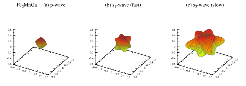
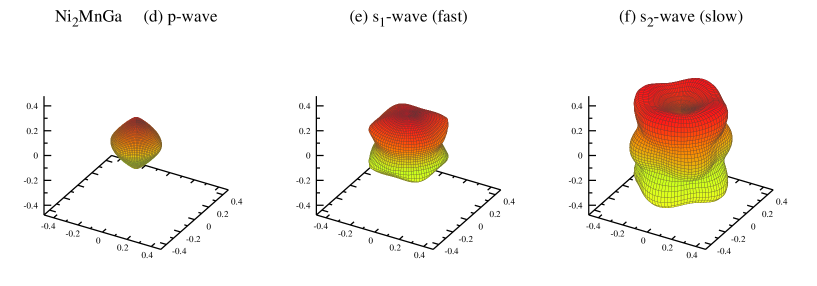
Figure 7: (Online color) Slowness surfaces of Fe₂MnGa (a)–(c) and Ni₂MnGa (d)–(f).
The slowness is given in (km/s)^-1.

Further material parameters are derived from the average sound velocities as described in Appendix C. At low temperatures, where only acoustic vibrational modes contribute, the Debye temperature $\theta_{\rm D}$ can be estimated from the average sound velocity Anderson (1963). The values estimated in this way are generally larger than Debye temperatures determined from phonon calculations or in experiments Ouardi et al. (2012) because the optical phonon branches are neglected when the elastic constants are used for calculating the “acoustical” Debye temperature $\theta_{\rm D}^{\rm acc}$. In a similar way, the average sound velocities can be used to estimate the “acoustical” Grüneisen parameter $\zeta^{\rm ac}$  Belomestnykh (2004).

The calculated average sound velocities together with the estimated Debye temperatures and Grüneisen parameters are listed in Table 5. The average sound velocities are rather similar for all compounds, ranging from about 3100 to 3800 m/s. The acoustical Debye temperatures are all above room temperature, ranging from 376 to 490 K. As expected, compounds consisting of heavier elements tend to have lower values. With the exception of Mn₂NiGa, all $\zeta^{\rm ac}$ values are about 2. This demonstrates that the anharmonicity of the lattice vibrations is nearly the same for all compounds.

As further shown in Table 5, the theory and experimental values have about a 20% discrepancy for the case of Ni₂MnGa. As reported in Reference [Chernenko et al., 2008], however, the stoichiometry of the compound has a large effect on the measured Debye temperature. As shown in Table 4, the Debye temperature decreases by about 20% in ^27.9Ni. However, in the calculations, the changes in stoichiometry are extremely small. The changes in the calculated values may be more evident with larger variations in the stoichiometry. For example, in experiments, the results change from 261 K in the case of Ni_49.6Mn_21.9Ga_28.5 to 345 K in the case of Ni_53.1Mn_26.6Ga_20.3. Therefore, having an ideal 2:1:1 system, like that assumed in most theories, is not easily possible or may even be impossible from an experimental standpoint. However, the estimation of measurable properties should provide information about the studied system and its potential for applications.

Table 5: Derived physical properties of tetragonal Heusler compounds.
Tabulated are the longitudinal $v_{l}$, transverse $v_{t}$, and average $\overline{v}$ sound velocities as well as the acoustical Debye temperature $\theta_{\rm D}^{\rm ac}$ and acoustical Grühneisen parameter $\zeta^{\rm ac}$ estimated from the sound velocities. All $v$ are given in ms^-1, $\theta$ is given in K, $\zeta$ is dimensionless.

Compound	$v_{l}$	$v_{t}$	$\overline{v}$	$\theta_{\rm D}^{\rm ac}$	$\zeta^{\rm ac}$
Mn2NiGa	5667	3441	3803	490	1.67
Ni2MnGa	5688	3219	3487	451	1.95
Exp.				345
Other calc.	5572	2853	3196	323
Mn2FeGa	5443	3023	3367	434	2.02
Fe2MnGa	5753	3253	3618	470	1.96
Rh2CrSn	5404	3078	3421	410	1.93
Rh2FeSn	5277	2803	3133	376	2.19
Rh2CoSn	5346	2885	3221	389	2.13

IV Summary

In the present work, the elastic constants of tetragonally distorted Heusler compounds were determined. The full-potential LAPW method together with the gradient-corrected PBE exchange-correlation functional were employed for all calculations. The relation between the calculated elastic constants and convergence criteria were discussed. Increasing only one of the parameters, such as the $k$-points or $R_{\rm MT}K_{\rm max}$, while keeping the other parameter low led to large errors in the calculated elastic constants. Therefore, to calculate both elastic constants accurately, $R_{\rm MT}K_{\rm max}$ and $k$-points must be sufficiently large to guarantee convergance. Structural optimization was shown to have an important effect on the elastic constants for tetragonal Heusler compounds. The method was used to investigate the crystalline stability of materials based on the calculation of their elastic properties.

Based on the calculated results, the considered tetragonal Heusler compounds are intermediate materials, between brittle and ductile. Elastically, they exhibit mainly metallic rather than covalent bonding. The structural instability, mechanical properties, structural anisotropy, and other mechanical properties were also explored. Using the virtual crystal approximation, the importance of the stoichiometric composition for Ni₂MnGa was demonstrated, and extreme sensitivity on the variation of the Ni component in Ni₂MnGa was observed. Negative anisotropy of ^27.9Ni₂MnGa and Ni₂Mn^30.9Ga together with the large anisotropy of the ^28.1Ni₂MnGa and Ni₂^25.1MnGa compounds indicated instability of off-stoichiometric Ni₂MnGa in the tetragonal phase.

The calculated material properties are useful for applications focusing on bulk materials. However, the appearance and prediction of metastable tetragonal structures allows lattice parameter engineering with artificial $c/a$ ratios initialized by epitaxial or pseudomorphic thin film growth. Thus, Heusler thin films could be designed to have specific properties.

Appendix A Basic equations for the elastic constants, moduli, and related parameters

The equations that describe the elastic properties of solids have been described in detail by Nye Nye (1985); this discussion is summarized here and compares tetragonal, hexagonal, and cubic systems with focus on the tetragonal case. The strain matrix $\epsilon$ transforms lattice $A$ with basis vectors $X,Y,Z$ into the deformed lattice

$$A^{\prime}=(\underline{1}+\epsilon)A$$ (8)

with basis vectors $X^{\prime},Y^{\prime},Z^{\prime}$. The symmetric strain matrix $\epsilon$ contains six different strains $e_{i}$ and has the form:

$$\underline{1}+\epsilon=\left(\begin{array}[]{ccc}1+e_{1}&\frac{1}{2}e_{6}&\frac{1}{2}e_{5}\\ \frac{1}{2}e_{6}&1+e_{2}&\frac{1}{2}e_{4}\\ \frac{1}{2}e_{5}&\frac{1}{2}e_{4}&1+e_{3}\\ \end{array}\right)$$ (9)

The elastic relations (Hooke’s law) between the strain ($\epsilon$) and stress ($\sigma$) matrices are mediated by the elastic compliance ($\bm{S}$) or the elastic stiffness ($\bm{C}$) matrices:

$$\epsilon={\bm{S}}\sigma\>\>{\rm or}\>\>\sigma={\bm{C}}\epsilon$$ (10)

From the elastic equations, the relations between the compliance matrix and the stiffness matrix are

$${\bm{S}}={\bm{C}}^{-1}$$ (11)

and vice versa ${\bm{C}}={\bm{S}}^{-1}$. These relations imply that ${\bm{SC}}={\bm{CS}}=\underline{1}$.

In the most general case, the elastic matrix is symmetric and of order $6\times 6$. In triclinic lattices, the elastic matrix contains 21 independent elastic constants. This number is largely reduced in high symmetry lattices. For example, in an isotropic system, it contains only the two constants $c_{11}=c_{22}=c_{33}$ and $c_{12}=c_{13}=c_{23}$, and the remaining diagonal elements of the matrix are determined by $c_{44}=c_{55}=c_{66}=(c_{11}-c_{12})/2$.

In cubic lattices, the three elastic constants $c_{11}$, $c_{12}$, and $c_{44}$ are independent. There are five independent elastic constants for hexagonal structures ($c_{11}$, $c_{12}$, $c_{13}$, $c_{33}$, and $c_{44}$), while tetragonal structures have either seven (classes: $4$, $\overline{4}$, or $4/m$) or six ($c_{11}$, $c_{12}$, $c_{13}$, ($c_{16}=-c_{15}$), $c_{33}$, $c_{44}$ and $c_{66}$) elastic constants. The elastic matrix for all classes of cubic and hexagonal crystals as well as the classes $4mm$, $\overline{4}2m$, $422$, or $4/mmm$ of tetragonal crystals have the form

$$C=\left(\begin{array}[]{ccc ccc}c_{11}&c_{12}&c_{13}&.&.&(c_{16})\\ c_{12}&c_{11}&c_{13}&.&.&(-c_{16})\\ c_{13}&c_{13}&c_{33}&.&.&.\\ .&.&.&c_{44}&.&.\\ .&.&.&.&c_{44}&.\\ (c_{16})&(-c_{16})&.&.&.&c_{66}\\ \end{array}\right)$$ (12)

where zero elements are assigned by dots and additional tetragonal elements for classes $4$, $\overline{4}$, or $4/m$ are given in brackets. Moreover, the elastic matrix has restrictions $c_{33}=c_{11}$, $c_{66}=c_{44}$, $c_{13}=c_{12}$ in cubic systems and $c_{66}=(c_{11}-c_{12})/2$ in hexagonal systems.

The matrix $C^{\rm tetra}$ has six eigenvalues for the classes $4mm$, $\overline{4}2m$, $422$, or $4/mmm$:

• $C_{1}^{t}=c_{11}-c_{12}$,

• $C_{2,3}^{t}=\frac{1}{2}\left(c_{11}+c_{33}+c_{12}\pm\sqrt{Z}\right)$

• $C_{4}^{t}=c_{66}$, and

• $C_{5,6}^{t}=c_{44}$,

where $Z=c_{11}^{2}+2c_{11}c_{12}-2c_{11}c_{33}+c_{12}^{2}-2c_{12}c_{33}+8c_{13}^{2}+c_{33}^{2}$. The last eigenvalue ($C_{5,6}^{t}$) is twofold degenerate (also note the double sign ($\pm$) in the second line). The crystal becomes unstable when one of the eigenvalues becomes zero or negative or in case that $Z<0$.

The relations between the elastic constants $c_{ij}$ and the elements of the compliance matrix $s_{ij}$ are found from Equation 11. In all classes of hexagonal systems or in tetragonal systems belonging to the classes $4mm$, $\overline{4}2m$, $422$, or $4/mmm$, the relations between $c_{ij}$ and $s_{ij}$ are given by

$$s_{11} = \frac{c_{11}c_{33}-c_{13}^{2}}{c(c_{11}-c_{12})}$$ (13)

$$s_{12} = \frac{-c_{12}c_{33}+c_{13}^{2}}{c(c_{11}-c_{12})}$$

$$s_{13} = \frac{-c_{13}}{c}$$

$$s_{33} = \frac{c_{11}+c_{12}}{c}$$

$$c = c_{33}(c_{11}+c_{12})-2c_{13}^{2}$$

$$s_{44} = \frac{1}{c_{44}}$$

$$s_{66} = \frac{1}{c_{66}}$$

where $c_{66}$ appears only in tetragonal systems. Indeed, the number of equations is much less in cubic systems as shown from the restrictions given above.

The elastic properties of single crystals are completely determined by the elastic matrices ${\bm{C}}$ and ${\bm{S}}$. In reality, polycrystalline materials are considered more often than single crystals. Polycrystalline materials consist of randomly oriented crystals, and thus, a description of their elastic properties requires only two independent elastic moduli: the bulk modulus ($B$) and the shear modulus ($G$). The relationships between the single-crystal elastic constants and the polycrystalline elastic moduli are given by the Voigt Voigt (1928) or Reuß Reuß (1929) averages. Voigt’s approach uses the elastic stiffnesses $c_{ij}$, while Reuß’s approach uses the compliances $s_{ij}$. Voigt’s moduli Voigt (1928) are given as function of the elastic constants by the equations:

$$B_{V} = \frac{1}{9}(2c_{11}+2c_{12}+4c_{13}+c_{33})$$ (14)

$$G_{V} = \frac{1}{15}(2c_{11}-c_{12}-4c_{13}+c_{33}+6c_{44}+3c_{66})$$

and Reuß’s moduli Reuß (1929) are usually calculated from the elements of the compliance matrix:

$$B_{R} = \frac{1}{2s_{11}+2s_{12}+4s_{13}+s_{33}}$$

$$= \frac{(c_{11}+c_{12})c_{33}-2c_{13}^{2}}{c_{11}+c_{12}+2c_{33}-4c_{13}}$$

$$G_{R} = \frac{15}{8s_{11}-4s_{12}-8s_{13}+4s_{33}+6s_{44}+3s_{66}}.$$

For cubic or isotropic crystals, the bulk moduli in Voigt’s ($B_{V}$) and Reuß’s ($B_{R}$) approach are equal, as shown by using the restrictions on $c_{ij}$ given above. In cases other than isotropic or cubic, $G_{R}$ cannot be easily rewritten in terms of the elastic constants.

Finally, the mechanical properties of polycrystalline materials are approximated in the Voigt–Reuß–Hill Hill (1952) approach, where the bulk and shear moduli are given by arithmetic averages:

$$B = \frac{1}{2}(B_{V}+B_{R})$$ (16)

$$G = \frac{1}{2}(G_{V}+G_{R}).$$

The bulk modulus $B$ of a material characterizes its resistance to fracture, whereas the shear modulus $G$ characterizes its resistance to plastic deformations. Therefore, ratios between the elastic moduli $B$ and $G$ are often given for characterization and comparison of different materials. Pugh’s modulus $k$ is the simple ratio of the bulk and shear moduli Pugh (1954):

$$k=B/G.$$ (17)

Poisson’s ratio $\nu$ also relates the bulk and shear moduli:

$$\nu=\frac{1}{2}\ \frac{3B-2G}{3B+G}=\frac{3k-2}{6k+2}.$$ (18)

Further, Poisson’s ratio bridges between the rigidity modulus $G$ and Young’s modulus $E$, which is given by

$$E=2G(1+\nu)=\frac{9BG}{3B+G}.$$ (19)

Appendix B Elastic stability and representation of elastic properties

The set of elastic moduli and their ratios allows characterization of the elastic behavior of materials. However, the mechanical stability is still open. As a first criterion, the elastic moduli all must be positive. Born and coworkers developed a theory on the stability of crystal lattices Born (1940); *Mis40; *BFu40; *BMi40; *Fue41a; *Fue41b; Born and Huang (1956). For tetragonal crystals at ambient conditions, the seven elastic stability criteria are given by

• $2c_{11}+c_{33}+2c_{12}+4c_{13}>0$

• $c_{11}+c_{33}-2c_{13}>0$

• $c_{12},c_{33},c_{44},c_{66}>0$

• $c_{11}-c_{12}>0$

Note that the number of criteria is reduced for the lower number of elastic constants in hexagonal or cubic crystals to 5 or 3, respectively. The last condition is used to define the tetragonal shear modulus $c^{\prime}=(c_{11}-c_{12})/2$. In some works, the direct difference $C^{\prime}=c_{11}-c_{12}$ is used. If external, hydrostatic pressure $p$ is applied, then the crystal becomes unstable when $2p>C^{\prime}$, that is, at $p>c^{\prime}$.

The linear compressibility $\beta$ is the crystal response to hydrostatic pressure by a length decrease. For cubic systems, the linear compressibility is isotropic, that is, a sphere of a cubic crystal under hydrostatic pressure remains a sphere. The situation is different in non-cubic systems where $\beta=\beta(\hat{r})$ becomes directionally dependent. In hexagonal, trigonal, and tetragonal systems, the directional dependence is given by

$$\beta(\hat{r})=(s_{11}+s_{12}+s_{13})(\hat{x}^{2}+\hat{y}^{2})-(s_{11}+s_{12}-s_{13}-s_{33})\hat{z}^{2}.$$ (20)

The linear compressibility of a cubic crystal is simply $\beta^{\rm cub}=s_{11}+2s_{12}$. The volume compressibility $\kappa$ of hexagonal and tetragonal systems is also directionally dependent and given in Reuß’s approach by

$$\kappa(\hat{r})= (s_{11}+s_{12}+s_{13})(\hat{x}^{2}+\hat{y}^{2})$$ (21)

$$+ (s_{33}+2s_{13})\hat{z}^{2}$$

For cubic systems, $s_{13}=s_{12}$ and $s_{33}=s_{11}$, that is, $\kappa^{\rm cub}=3(s_{11}+2s_{12})$, and thus, the bulk modulus $B=1/\kappa$ is isotropic for crystals with cubic symmetry. For hexagonal and tetragonal systems, $\kappa$ becomes isotropic when the two terms $s_{11}+s_{12}+s_{13}$ and $s_{33}+2s_{13}$ in Equation 21 are equal. Therefore, the anisotropy of the hexagonal and tetragonal bulk moduli is defined by

$$A_{B}=\frac{s_{33}+2s_{13}}{s_{11}+s_{12}+s_{13}},$$ (22)

and their isotropic compressibility becomes $\kappa^{\rm hex,tet}_{\rm iso}=2s_{11}+s_{33}+2s_{12}+4s_{13}$.

Other than the bulk modulus of cubic crystals, Young’s modulus of cubic, hexagonal, or tetragonal systems is not isotropic. The representation surface of Young’s modulus for tetragonal systems with classes $4mm$, $422$, $\overline{4}2m$, and $4/mmm$ is given by

$$\frac{1}{E^{t}(\hat{r})}= (\hat{x}^{4}+\hat{y}^{4})s_{11}+\hat{z}^{4}s_{33}$$ (23)

$$+ \hat{x}^{2}\hat{y}^{2}(2s_{12}+s_{66})$$

$$+ \hat{z}^{2}(1-\hat{z}^{2})(2s_{13}+s_{44}).$$

For the tetragonal classes $4$, $4/m$, and $\overline{4}$, an additional term is present such that

$$\frac{1}{E^{t^{\prime}}(\hat{r})}=\frac{1}{E^{t}(\hat{r})}+2\hat{x}\hat{y}(\hat{x}^{2}-\hat{y}^{2})s_{16}.$$ (24)

The shear anisotropic factors provide a measure of the degree of anisotropy in the bonding between atoms in different planes. The number of different shear anisotropies depends on the crystal system. In both – hexagonal and tetragonal – systems, the shear anisotropic factors $A_{100}$ (or equivalent $A_{010}$) for the $\{100\}$ shear planes between the $\left\langle 011\right\rangle$ and $\left\langle 010\right\rangle$ directions and $A_{001}$ for the $\{001\}$ planes between $\left\langle 110\right\rangle$ and $\left\langle 010\right\rangle$ are:

$$A_{100} = \frac{4c_{44}}{c_{11}+c_{33}-2c_{13}}$$

$$A_{001} = \frac{2c_{66}}{c_{11}-c_{12}}$$ (25)

In cubic crystals, both factors are the same $A_{e}=A_{001}=2c_{44}/(c_{11}-c_{12})$, as mentioned above. In hexagonal systems, $c_{66}=(c_{11}-c_{12})/2$, and thus, $A_{001}=1$. For isotropic crystals, all $A$ factors must be unity, while any value smaller or greater than unity is a measure of the degree of elastic anisotropy possessed by the crystal.

Comparing the equations (22,25) for the elastic anisotropies with the Born–Huang Born and Huang (1956) criteria, these equations can clearly be used to show the elastic stability. Most obviously, crystals with one negative anisotropy are not stable. Further, crystals with large anisotropies also tend to instabilities; in particular, crystals are not stable for $A\rightarrow\infty$ when one of the denominators becomes zero. This behavior makes the anisotropies important parameters, even though they may not cover all possible causes for Born–Huang instabilities.

Appendix C Equations for calculating properties from the elastic constants

Besides the elastic moduli, further important physical quantities can be derived from the elastic constants. Acoustical spectroscopy is widely used to determine the elastic properties of crystalline solids. The propagation of sound waves in solids is described by the Christoffel equation:

$$(\Gamma_{ij}-\rho v^{2}\delta_{ij})U_{j}=0,$$ (26)

where $v$ is the phase velocity, $\rho$ is the mass density, $\delta_{ij}$ is the Kronecker delta, $U$ is the polarisation vector, and

$$\Gamma_{ij}=c_{ijkl}l_{j}l_{l}$$ (27)

is the Christoffel tensor built from the elastic constants and the direction cosines $l_{i}$ ($i=1\ldots 3$) that describe the direction of wave motion. For tetragonal systems, the Christoffel tensor is given by

$$\Gamma_{11} = c_{11}l_{1}^{2}+c_{66}l_{2}^{2}+c_{44}l_{3}^{2}+2c_{16}l_{1}l_{2}$$ (28)

$$\Gamma_{22} = c_{66}l_{1}^{2}+c_{11}l_{2}^{2}+c_{44}l_{3}^{2}-2c_{16}l_{1}l_{2}$$

$$\Gamma_{33} = c_{44}l_{1}^{2}+c_{44}l_{2}^{2}+c_{33}l_{3}^{2}$$

$$\Gamma_{12} = c_{16}l_{1}^{2}-c_{16}l_{2}^{2}+(c_{12}+c_{66})l_{1}l_{2}-c_{16}l_{2}l_{3}$$

$$\Gamma_{13} = (c_{13}+c_{44})l_{1}l_{3}$$

$$\Gamma_{23} = (c_{13}+c_{44})l_{2}l_{3}$$

and $\Gamma_{ij}=\Gamma_{ji}$. The Christoffel tensor reduces for the classes $4mm$, $\overline{4}2m$, $422$, and $4/mmm$, where $c_{16}=0$, to

$$\Gamma_{11} = c_{11}l_{1}^{2}+c_{66}l_{2}^{2}+c_{44}l_{3}^{2}$$ (29)

$$\Gamma_{22} = c_{66}l_{1}^{2}+c_{11}l_{2}^{2}+c_{44}l_{3}^{2}$$

$$\Gamma_{33} = c_{44}l_{1}^{2}+c_{44}l_{2}^{2}+c_{33}l_{3}^{2}$$

$$\Gamma_{12} = (c_{12}+c_{66})l_{1}l_{2}$$

$$\Gamma_{13} = (c_{13}+c_{44})l_{1}l_{3}$$

$$\Gamma_{23} = (c_{13}+c_{44})l_{2}l_{3}$$

The solution of the characteristic $3\times 3$ matrix results in a third-order equation in $v^{2}$ for the phase velocity. Three distinct modes appear, one with longitudinal and two with transversal polarisation. Due to possible mixing, these modes are often referred to as quasi-longitudinal or quasi-transversal modes. The longitudinal mode corresponds to a pressure ($p$-wave) or compression wave as it appears also in gases. On the other hand, the transversal modes appear for solids, and they are distinguished as fast ($s_{1}$) and slow ($s_{2}$-wave) shear waves. The wave properties are presented as slowness surfaces.

The elastic constants also allow direct estimation of the averaged sound velocity $\overline{v}$ from the longitudinal ($v_{l}$) and transverse ($v_{t}$) elastic wave velocities of isotropic materials, which are given by

$$v_{l} = \sqrt{\frac{3B+4G}{3\rho}}$$ (30)

$$v_{t} = \sqrt{\frac{G}{\rho}},$$

where $\rho$ is the mass density of the material. Here, $\overline{v}$ is approximately predicted by

$$\overline{v}=\left[\frac{3}{v_{l}^{-3}+2v_{t}^{-3}}\right]^{1/3}.$$ (31)

For low temperatures, where only acoustic vibrational modes contribute, the Debye temperature $\Theta_{D}$ can be estimated from the average sound velocity using the relation Anderson (1963):

$$\Theta^{\rm ac}_{D}=\overline{v}\frac{h}{k_{B}}\sqrt[3]{\frac{f}{4\pi}\frac{N_{A}\rho}{M}}=\overline{v}\frac{h}{k_{B}}\sqrt[3]{\frac{f}{4\pi}\frac{1}{V_{p}}},$$ (32)

where $h$, $k_{B}$, and $N_{A}$ are Plank’s constant, Boltzman’s constant, and Avogadoro’s number, respectively. The degree of freedom for $n$ atoms in a primitive cell with volume $V_{p}$ ($f=12$ for Heusler compounds with $L2_{1}$ structure) is $f=3n$, and $M$ is the molecular mass, that is, the sum of all masses of the atoms in the primitive cell of the compound.

In solids, the Grüneisen parameter $\zeta$ is a measure of the anharmonicity of the interactions between the atoms. In general, it is calculated from logarithmic derivatives of the vibrational frequencies with respect to the crystal volume. However, full phonon calculations as function of crystal volumes are demanding tasks, and fast estimates are thus welcome. Belomestnykh Belomestnykh (2004) derived an “acoustical” Grüneisen parameter $\zeta^{\rm ac}$ that is directly related to the sound velocities. Therefore, $\zeta^{\rm ac}$ is given by

$$\zeta^{\rm ac}=\frac{3}{2}\frac{(3v_{l}^{2}-4v_{t}^{2})}{(v_{l}^{2}+2v_{t}^{2})}.$$ (33)

References

- Graf et al. (2011) T. Graf, C. Felser, and S. S. P. Parkin, Prog. Solid State Chem. 39, 1 (2011).
- Winterlik et al. (2009) J. Winterlik, G. H. Fecher, A. Thomas, and C. Felser, Phys. Rev. B 79, 064508 (2009).
- van Hove (1953) L. van Hove, Phys. Rev. 89, 1189 (1953).
- Brown et al. (1999) P. Brown, A. Bargawi, J. Crangle, K.-U. Neumann, and K. Ziebeck, J. Phys.: Condens. Matter 11, 4715 (1999).
- Blum et al. (2011) C. G. F. Blum, S. Ouardi, G. H. Fecher, B. Balke, X. Kozina, G. Stryganyuk, S. Ueda, K. Kobayashi, C. Felser, S. Wurmehl, and B. Büchner, Appl. Phys. Lett. 98, 252501 (2011).
- Winterlik et al. (2008) J. Winterlik, B. Balke, G. H. Fecher, C. Felser, M. C. M. Alves, F. Bernardi, and J. Morais, Phys. Rev. B 77, 054406 (2008).
- Krén and Kádár (1970) E. Krén and G. Kádár, Solid State Communications 8, 1653 (1970).
- Wu et al. (2009) F. Wu, S. Mizukami, D. Watanabe, H. Naganuma, M. Oogane, Y. Ando, and T. Miyazaki, Appl. Phys. Lett. 94, 122503 (2009).
- Wu et al. (2010) F. Wu, S. Mizukami, D. Watanabe, E. Sajitha, H. Naganuma, and M. Oogane, IEEE Trans. Magn. 46, 1863 (2010).
- Gilleßen and Dronskowski (2010) M. Gilleßen and R. Dronskowski, J. Comput. Chem. 31, 612 (2010).
- Gilman (2009) J. J. Gilman, Chemistry and Physics of Mechanical Hardness (J. Wiley and Sons, Inc, Hoboken, New Jersey, 2009).
- Gilman (2001) J. J. Gilman, Electronic basis of the strength of materials (Cambridge University Press, Cambridge, 2001).
- (13) K. D. S. (Ed.), Chemical hardness (Springer-Verlag, Berlin, 1997).
- Bruls et al. (1994) G. Bruls, B. Wolf, D. Finsterbusch, P. Thalmeier, I. Kouroudis, W. Sun, W. Assmus, B. Lüthi, M. Lang, K. Gloos, F. Steglich, and R. Modler, Phys. Rev. Lett. 72, 1754 (1994).
- Ledbetter et al. (1989) H. M. Ledbetter, S. A. Kim, R. B. Goldfarb, and K. Togano, Phys. Rev. B 39, 9689 (1989).
- Gilman (1960) J. J. Gilman, Aust. J. Phys. 13, 327 (1960).
- Li et al. (2013) J. Li, Z. Zhang, Y. Sun, J. Zhang, G. Zhou, H. Luo, and G. Liu, Physica B: Condensed Matter 409, 35 (2013).
- Li et al. (2012) C.-M. Li, H.-B. Luo, Q.-M. Hu, R. Yang, B. Johansson, and L. Vitos, Phys. Rev. B 86, 214205 (2012).
- Luo et al. (2012) H.-B. Luo, Q.-M. Hu, C.-M. Li, R. Yang, B. Johansson, and L. Vitos, Phys. Rev. B 86, 024427 (2012).
- Li et al. (2011a) C.-M. Li, H.-B. Luo, Q.-M. Hu, R. Yang, B. Johansson, and L. Vitos, Phys. Rev. B 84, 174117 (2011a).
- Li et al. (2011b) C.-M. Li, H.-B. Luo, Q.-M. Hu, R. Yang, B. Johansson, and L. Vitos, Phys. Rev. B 84, 024206 (2011b).
- Hu et al. (2009a) Q.-M. Hu, C.-M. Li, R. Yang, S. E. Kulkova, D. I. Bazhanov, B. Johansson, and L. Vitos, Phys. Rev. B 79, 144112 (2009a).
- Moya et al. (2006) X. Moya, L. Ma nosa, A. Planes, T. Krenke, M. Acet, M. Morin, J. L. Zarestky, and T. A. Lograsso, Phys. Rev. B 74, 024109 (2006).
- Bungaro et al. (2003) C. Bungaro, K. M. Rabe, and A. D. Corso, Phys. Rev. B 68, 134104 (2003).
- de Jong et al. (2012) M. de Jong, D. L. Olmsted, A. van de Walle, and M. Asta, Phys. Rev. B 86, 224101 (2012).
- Suits (1976) J. C. Suits, Solid State Communications 18, 423 (1976).
- Wu et al. (2017) S. Wu, S. S. Naghavi, G. H. Fecher, and C. Felser, arxive cond-mat 00, 00000 (2017).
- Ziambaras and Schröder (2003) E. Ziambaras and E. Schröder, Phys. Rev. B 68, 064112 (2003).
- Birch (1947) F. Birch, Phys. Rev. 71, 809 (1947).
- Murnaghan (1944) F. D. Murnaghan, Proc. Natl. Acad. Sci. 30, 244 (1944).
- Wallace (1972) D. C. Wallace, Thermodynamics of Crystals (Dover Publication Inc., Mineola, New York, 1972).
- Kart et al. (2008) S. O. Kart, M. Uludoğan, I. Karaman, and T. Çağ ın, Phys. Status Solidi (a) 205, 1026 (2008).
- Blaha et al. (2001) P. Blaha, K. Schwarz, G. Madsen, D. Kvasnicka, and J. Luitz, Wien2k (2001).
- Graf et al. (2009) T. Graf, G. H. Fecher, J. Barth, J. Winterlik, and C. Felser, J. Phys. D: Appl. Phys. 42, 084003 (2009).
- Ishida et al. (1982) S. Ishida, S. Akazawa, Y. Kubo, and J. Ishida, J. Phys. F: Met. Phys. 12, 1111 (1982).
- Mohn et al. (1995) P. Mohn, P. Blaha, and K. Schwarz, J. Magn. Magn. Mater. 140–144, 183 (1995).
- Perdew et al. (1997) J. P. Perdew, K. Burke, and M. Ernzerhof, Phys. Rev. Lett. 78, 1396 (1997).
- Perdew et al. (1996) J. P. Perdew, K. Burke, and M. Ernzerhof, Phys. Rev. Lett. 77, 3865 (1996).
- Kart and Çağ ın (2010) S. O. Kart and T. Çağ ın, J. Alloys Compd. 508, 177 (2010).
- Martynov and Kokorin (1992) V. V. Martynov and V. V. Kokorin, J. Phys. III 2, 739 (1992).
- Webster et al. (1984) P. J. Webster, K. R. A. Ziebeck, S. L. Town, and M. S. Peak, Philos. Mag. B 49, 295 (1984).
- Tsunegi et al. (2008) S. Tsunegi, Y. Sakuraba, M. Oogane, K. Takanashi, and Y. Ando, Appl. Phys. Lett. 93, 112506 (2008).
- Worgull et al. (1996) J. Worgull, E. Petti, and J. Trivisonno, Phys. Rev. B 54, 15695 (1996).
- Hu et al. (2009b) Q.-M. Hu, C.-M. Li, R. Yang, S. E. Kulkova, D. I. Bazhanov, B. Johansson, and L. Vitos, Phys. Rev. B 79, 144112 (2009b).
- Ledbetter (2006) H. Ledbetter, Mater. Sci. Eng., A 442, 31 (2006).
- Dhar et al. (1980) S. K. Dhar, A. K. Grover, S. K. Malik, and R. Vijayaraghavan, Solid State Communications 33, 545 (1980).
- Pugh (1954) S. F. Pugh, Phil. Mag. 45, 823 (1954).
- McSkimin and Bond (1957) H. J. McSkimin and W. L. Bond, Phys. Rev. 105, 116 (1957).
- Lazarus (1949) D. Lazarus, Phys. Rev. 76, 545 (1949).
- Niu et al. (2012) H. Niu, X.-Q. Chen, P. Liu, W. Xing, X. Cheng, D. Li, and Y. Li, Sci. Rep. 2 (2012).
- Christensen (2013) R. M. Christensen, The Theory of Materials Failure (Oxford University Press, Oxford, 2013).
- Bader (1990) R. F. W. Bader, Atoms in Molecules. A Quantum Theory (Oxford University Press, Oxford, 1990).
- Otero-de-la Roza et al. (2009) A. Otero-de-la Roza, M. A. Blanco, A. M. Pendas, and V. Luana, Comp. Phys. Comm. 180, 157 (2009).
- Otero-de-la Roza et al. (2014) A. Otero-de-la Roza, E. R. Johnson, and V. Luana, Comp. Phys. Comm. 185, 1007 (2014).
- Zayak and Entel (2004) A. Zayak and P. Entel, Mater. Sci. Eng., A 378, 419 (2004).
- Jiang et al. (2003) C. Jiang, S. Gong, and H. Xu, Mater. Sci. Eng., A 342, 231 (2003).
- Gasi et al. (2013) T. Gasi, V. Ksenofontov, J. Kiss, S. Chadov, A. K. Nayak, M. Nicklas, J. Winterlik, M. Schwall, P. Klaer, P. Adler, and C. Felser, Phys. Rev. B 87, 064411 (2013).
- Anderson (1963) O. L. Anderson, J. Phys. Chem. Solids 24, 909 (1963).
- Ouardi et al. (2012) S. Ouardi, G. H. Fecher, C. Felser, M. Schwall, S. S. Naghavi, A. Gloskovskii, B. Balke, J. Hamrle, K. Postava, J. Pištora, S. Ueda, and K. Kobayashi, Phys. Rev. B 86, 045116 (2012).
- Belomestnykh (2004) V. N. Belomestnykh, Tech. Phys. Lett. 30, 91 (2004).
- Chernenko et al. (2008) V. Chernenko, A. Fujita, S. Besseghini, and J. Pérez-Landazabal, J. Magn. Magn. Mater. 320, e156 (2008).
- Nye (1985) J. F. Nye, Physical Properties of Crystals (Oxford Science Publications, Oxford, 1985).
- Voigt (1928) W. Voigt, Lehrbuch der Kristallphysik (Teubner Verlag, Leipzig, 1928).
- Reuß (1929) A. Reuß, Ztschr. f. angew. Math. und Mech. 9, 49 (1929).
- Hill (1952) R. Hill, Proc. Phys. Soc. A65, 349 (1952).
- Born (1940) M. Born, Proc. Camb. Phil. Soc. Math. Phys. Sci 36, 160 (1940).
- Misra (1940) R. D. Misra, Proc. Camb. Phil. Soc. Math. Phys. Sci 36, 173 (1940).
- Born and Fürth (1940) M. Born and R. Fürth, Proc. Camb. Phil. Soc. Math. Phys. Sci 36, 454 (1940).
- Born and Misra (1940) M. Born and R. D. Misra, Proc. Camb. Phil. Soc. Math. Phys. Sci 36, 466 (1940).
- Fürth (1941) R. Fürth, Proc. Camb. Phil. Soc. Math. Phys. Sci 37, 34 (1941).
- Fürth (1941) R. Fürth, Proc. Camb. Phil. Soc. Math. Phys. Sci 37, 177 (1941).
- Born and Huang (1956) M. Born and K. Huang, Dynamical Theory of Crystal Lattices (Clarendon Press, Oxford, 1956).