Heat fluctuations of Brownian oscillators in nonstationary processes:
fluctuation theorem and condensation transition

Abstract

We study analytically the probability distribution of the heat released by an ensemble of harmonic oscillators to the thermal bath, in the nonequilibrium relaxation process following a temperature quench. We focus on the asymmetry properties of the heat distribution in the nonstationary dynamics, in order to study the forms taken by the Fluctuation Theorem as the number of degrees of freedom is varied. After analysing in great detail the cases of one and two oscillators, we consider the limit of a large number of oscillators, where the behavior of fluctuations is enriched by a condensation transition with a nontrivial phase diagram, characterized by reentrant behavior. Numerical simulations confirm our analytical findings. We also discuss and highlight how concepts borrowed from the study of fluctuations in equilibrium under symmetry breaking conditions [Gaspard, J. Stat. Mech. P08021 (2012)] turn out to be quite useful in understanding the deviations from the standard Fluctuation Theorem.

I Introduction

At the level of the thermodynamical description of out of equilibrium transformations, the irreversibility of macroscopic processes is encoded in the second law expressed through strict inequalities satisfied by various thermodynamic observables, like entropy and free energies. At the more refined level of the statistical mechanical description of the same processes, the irreversibility ought to manifest as an asymmetry in the probability distributions of the fluctuations of these same quantities. The central and yet unsolved problem is to find general methods, comparable to those available in equilibrium, to characterize these probability distributions. A major advance in this direction has been made in the last two decades with the development of Fluctuations Theorems (FT), which allow to constrain the form of the distributions with a certain degree of universality and in conditions arbitrarily far from equilibrium Seifert . This theoretical approach turned out to be very useful, both in experimental and numerical studies, in the characterization of several nonequilibrium systems, such as colloidal particles in harmonic traps Wang ; Zon ; imparato07 ; kim , vibrated granular media Sarracino ; Naert ; Gnoli , models of coupled Langevin equations Farago ; Joubaud ; Crisanti , driven stochastic Lorentz gases Gradenigo ; Gradenigo2 , and active matter Kumar , just to name a few examples.

An important development in the field has been achieved with the understanding of the impact of symmetry and symmetry breaking on the FT of currents in stationary diffusive systems Hurtado . More recently, it has been shown that relations in the form of FT are of general occurrence also in the probability distributions of order parameters in equilibrium statistical mechanics, in connection with symmetry breaking Gaspard . Here we show that these equilibrium results do feedback in the understanding of the nonequilibrium FT, shedding new light on the conditions under which the FT in the standard form (namely, with a linear asymmetry function) is expected to hold Puglisi ; Baiesi ; Harris ; Park . In particular, we study the fluctuations of the heat exchanged with the environment by one or more Brownian oscillators in an interval of time $[t_{w},t]$, during the relaxation following the instantaneous quench from high to low temperature. This protocol induces a nonstationary dynamics that is noninvariant under time translation and therefore the heat exchanged along a given trajectory explicitly depends on the two times $(t_{w},t)$. The study of the FT in similar processes has been addressed in Ritort ; Picco ; Zamponi . Here, we derive exact expressions for the heat probability density functions, for one, two and a large number of independent oscillators. Our analysis shows how, in the case of more than one oscillator, the heat probability obeys an FT which deviates from the standard form and whose physical meaning can be rationalized by resorting to the analogy with the equilibrium problem in the presence of a nonuniform external field.

In the case of a large number of degrees of freedom, arising, for instance, in the normal mode decomposition of an extended system, we present a computation based on the steepest descent method, which allows us to obtain an accurate description of the large deviation function of the exchanged heat. Here, we will use large deviation theory with a large number of degrees of freedom (and not for long time intervals) hugo ; ld . This kind of problem was considered previously in Refs. Gonnella ; Jo ; Pechino , showing that fluctuations undergo a condensation transition. Briefly, by this is meant that fluctuations in a multi-component system do condense if there exists a critical threshold above which the fluctuation is feeded by just one of the components (or degrees of freedom). Here, we analyse in detail the crossover region between the normal and the condensed phase, providing an explicit expression for the large deviation function. We also reconstruct numerically the phase diagram at finite temperature, in the parameter space $(t_{w},\tau=t-t_{w})$, which shows a nontrivial reentrant behavior.

The paper is organized as follows. In Section II we present the general framework within which various FT forms are derived and we argue on physical grounds for the particular form we adopt. We also recall in some detail how an FT arises in statics as a consequence of symmetry breaking, highlighting its relevance for the dynamical problem. Section III is devoted to the simplest case of a single oscillator. We compute exactly the probability distribution of heat fluctuations, we introduce the basic concept of time-dependent effective temperature and we derive the FT in the “Gallavotti-Cohen” form Gallavotti . In Section IV we consider the case of two oscillators, and we analyse the modifications arising in the FT form due to the presence of more than one degree of freedom. In Section V we consider the case of a large number of oscillators. We discuss the conditions leading to condensation and we map out numerically the phase diagram in the parameter space. The consequences on the FT are analysed. Finally, conclusions are drawn in Section VI.

II General setup

There exist many variants of FT whose derivation Maes ; Seifert ; Gawedzki can be unified into a single master theorem. Let us first outline the general setting which applies to all fluctuation problems, in or out of equilibrium. Consider a sample space $\Omega$ with elements $\sigma$. Let $\mu(\sigma)$ and $\mu^{\prime}(\sigma)$ be two arbitrary probability measures over $\Omega$ and let ${\cal W}(\sigma)$ be defined by

$$\frac{\mu^{\prime}(\sigma^{*})}{\mu(\sigma)}=e^{-{\cal W}(\sigma)},$$ (1)

where the $*$ operation denotes an involutory transformation of $\Omega$ onto itself, i.e. $(\sigma^{*})^{*}=\sigma$. In the following this will be taken as the representation of the inversion element of the $\mathbb{Z}_{2}=(\mathbb{I},*)$ group, where $\mathbb{I}$ is the identity operator. Introducing an arbitrary function ${\cal F}(\sigma)$, from the above relation there follows the identity

$$\langle{\cal F}(\sigma)e^{-{\cal W}(\sigma)}\rangle=\langle{\cal F}(\sigma^{*})\rangle^{\prime},$$ (2)

where $\langle\cdot\rangle$ and $\langle\cdot\rangle^{\prime}$ denote expectations with respect to $\mu(\sigma)$ and $\mu^{\prime}(\sigma)$, respectively. Taking for ${\cal F}(\sigma)$ the characteristic function $\theta_{{\cal M}}(\sigma|M)$ of a certain observable ${\cal M}(\sigma)$, that is

$$\theta_{{\cal M}}(\sigma|M)=\left\{\begin{array}[]{ll}1,\;\;$if$\;\;{\cal M}(\sigma)=M,\\ 0,\;\;$if$\;\;{\cal M}(\sigma)\neq M,\end{array}\right.$$ (3)

from Eq. (2) follows

$$\frac{P^{\prime}({\cal M}(\sigma^{*})=M)}{P({\cal M}(\sigma)=M)}=\langle e^{-{\cal W}(\sigma)}|{\cal M}(\sigma)=M\rangle,$$ (4)

where $P^{\prime}$ and $P$ are the probabilities of the events in the arguments induced by $\mu^{\prime}(\sigma)$ and $\mu(\sigma)$, respectively, and in the right hand side there appears the expectation with respect to $\mu(\sigma)$, conditioned to ${\cal M}(\sigma)=M$. Defining the $*$ transformation on the set of random variables by ${\cal M}(\sigma)\mapsto{\cal M}^{*}(\sigma)={\cal M}(\sigma^{*})$, which is also an involution, the above relation can be recast in the form

$$\frac{P^{\prime}({\cal M}^{*}=M)}{P({\cal M}=M)}=e^{-{\cal K}(M)},$$ (5)

with

$${\cal K}(M)=-\ln\langle e^{-{\cal W}(\sigma)}|{\cal M}(\sigma)=M\rangle.$$ (6)

It appears, then, that Eq. (5) is the transposition to the level of the observable ${\cal M}$ of the underlying basic relation (1). In particular, regarding ${\cal W}$ as the bias which is necessary to apply on $\mu$ in order to construct $\mu^{\prime}$ and ${\cal K}$ as the analogous quantity relating $P$ and $P^{\prime}$, Eq. (6) tells how these biases are related one to the other.

As long as $\mu(\sigma)$ and $\mu^{\prime}(\sigma)$ are arbitrary, the above result does not have predictive power. It becomes the master FT when $\mu^{\prime}(\sigma)$ is taken with a definite relation to $\mu(\sigma)$, which constrains the form of $P(M)$ if the right hand side of Eq. (5) is accessible without having to actually compute the expectation, possibly via symmetry arguments. In the simplest case $\mu^{\prime}(\sigma)$ is taken to be the same as $\mu(\sigma)$. Then, from Eq. (1) one has

$$\frac{\mu(\sigma^{*})}{\mu(\sigma)}=e^{-{\cal W}(\sigma)},$$ (7)

showing that ${\cal W}$ is odd ${\cal W}(\sigma^{*})=-{\cal W}(\sigma)$ and characterizes the asymmetry of the probability measure under inversion. Now, the question is to what extent this asymmetry is preserved or distorted as the description is moved up from the microscopic level to the higher one of random variables. The answer from Eq. (5) is given by

$$\frac{P({\cal M}^{*}=M)}{P({\cal M}=M)}=e^{-{\cal K}(M)}.$$ (8)

Taking ${\cal M}$ to have definite parity, if it is even no information about the symmetry of $P$ is obtained and Eq. (8) yields the conditional integral FT

$$\langle e^{-{\cal W}(\sigma)}|{\cal M}(\sigma)=M\rangle=1.$$ (9)

Conversely, if ${\cal M}$ is odd, one has

$$\frac{P({\cal M}=-M)}{P({\cal M}=M)}=e^{-{\cal K}(M)},$$ (10)

whose usefulness depends on the possibility of assessing the form of ${\cal K}(M)$, which is called the asymmetry function (AF). In particular, if ${\cal M}\propto{\cal W}$, there follows an FT of the Gallavotti-Cohen Gallavotti form with a linear AF

$${\cal K}(M)\propto M.$$ (11)

If, instead, ${\cal W}$ and ${\cal M}$ are not simply related, the meaning of ${\cal K}(M)$ in general is not immediately transparent. For an overview of the variety of the different FT forms arising in the general case see Ref. Seifert .

II.1 FT and symmetry breaking in equilibrium

The latter remarks are well clarified in the equilibrium context, used in Ref. Gaspard to investigate the relation between FT and symmetry breaking. Let $\Omega$ and $\sigma$ be the system’s phase space and configurations, respectively. For definiteness, let $\sigma=(s_{1},...,s_{N})$, with $s_{i}=\pm 1$, be a spin configuration of a magnetic system on the lattice in the presence of an external site dependent field $\mathbb{B}=\{B_{i}\}$, whose equilibrium state is described by the probability measure

$$\mu(\sigma)=\mu_{0}(\sigma)e^{\beta\sum_{i}B_{i}s_{i}},$$ (12)

where $\mu_{0}(\sigma)$ is symmetric under spin inversion $\sigma^{*}=(-s_{1},...,-s_{N})$, while the exponential term breaks explicitly the $\mathbb{Z}_{2}$ symmetry. We are interested in the fluctuations of the global magnetization ${\cal M}(\sigma)=\sum_{i}s_{i}$. From Eq. (12) follows

$${\cal W}(\sigma)=2\beta\sum_{i}B_{i}s_{i},$$ (13)

and

$${\cal K}(M)=-\ln\langle e^{-2\beta\sum_{i}B_{i}s_{i}}|{\cal M}=M\rangle,$$ (14)

which takes a simple form only if the external field is uniform $B_{i}=B,\forall i$, yielding an FT with the linear AF Gaspard

$${\cal K}(M)=2\beta BM.$$ (15)

Instead, if $\mathbb{B}$ is not uniform, deviations from the FT arise. In order to take a closer look, let the number of spins to become large and consider the case of the ideal paramagnet, in which $\mu_{0}(\sigma)$ in Eq. (12) is the uniform measure $Z^{-1}=[\prod_{i}2\cosh(\beta B_{i})]^{-1}$. Then, by a straightforward saddle point computation one obtains the large deviation principle

$$P(M)\sim e^{-NI(m)},$$ (16)

where $m=M/N$ is the magnetization per spin and the large deviation function is given by

$$I(m)=x^{*}(m)m+\beta\bigl{[}f\bigl{(}\mathbb{B}^{*}(m)\bigr{)}-f(\mathbb{B})\bigr{]}.$$ (17)

Here,

$$f(\mathbb{B})=\lim_{N\to\infty}-\frac{1}{N\beta}\sum_{i}\ln[2\cosh(\beta B_{i})],$$ (18)

is the Helmotz free energy density, which depends on the field configuration $\mathbb{B}$, we have defined $\mathbb{B}^{*}(m)=\{B^{*}_{i}(m)\}$ with

$$B^{*}_{i}(m)=B_{i}+\beta^{-1}x^{*}(m),$$ (19)

and $x^{*}(m)$ is obtained by solving with respect to $x$ the equation of state

$$m = -\frac{\partial}{\partial x}f\bigl{(}\{B_{i}+\beta^{-1}x\}\bigr{)}$$ (20)

$$= \frac{1}{N}\sum_{i}\tanh(B_{i}+\beta^{-1}x).$$

Consequently, $\beta^{-1}x^{*}(m)$ is the shift to be applied to the external field on each site in order to produce $m$ as the average magnetization per spin. From the definition (10) follows

$$\frac{1}{N}{\cal K}(M)=I(-m)-I(m)$$

$$= -\bigl{[}x^{*}(-m)+x^{*}(m)\bigr{]}m+\beta\bigl{[}f\bigl{(}\mathbb{B}^{*}(-m)\bigr{)}-f\bigl{(}\mathbb{B}^{*}(m)\bigr{)}\bigr{]}.$$

Averaging Eq. (19) over $i$, we can write

$$\beta^{-1}x^{*}(m)=\overline{\mathbb{B}^{*}(m)}-\overline{\mathbb{B}},$$ (22)

with

$$\overline{\mathbb{B}^{*}(m)}=\frac{1}{N}\sum_{i}B^{*}_{i}(m),\,\,\,\overline{\mathbb{B}}=\frac{1}{N}\sum_{i}B_{i},$$ (23)

and Eq. (LABEL:G.5) can be put in the form

$$\frac{1}{N}{\cal K}(M)=2\beta\overline{\mathbb{B}}m+\beta\bigl{[}g(-m)-g(m)\bigr{]},$$ (24)

where we have defined

$$g(m)=f\bigl{(}\mathbb{B}^{*}(m)\bigr{)}+\overline{\mathbb{B}^{*}(m)}m.$$ (25)

In the particular case of the uniform external field

$$\overline{\mathbb{B}}=B,$$

$$B^{*}_{i}(m)=B^{*}(m)=B+\beta^{-1}x^{*}(m),\,\,\,\forall i,$$

$$\overline{\mathbb{B}^{*}(m)}=B^{*}(m),$$ (26)

and

$$g(m)=f(B^{*})+B^{*}m$$ (27)

is the Legendre transform of $f(B)$, which is even under $m$ reversal, since $B^{*}(m)$ is odd. Hence, in this case Eq. (24) reproduces the result (15). In the nonuniform case $g(m)$ is not the Legendre transform of $f(\mathbb{B})$ and in general does not have a definite parity, leading to a nonlinear AF function. We will come back on this point in Section IV. What the above exercise shows is that the FT, in the sense of a linear AF, holds as long as the macrovariable ${\cal M}$, whose fluctuations are considered, is conjugate to the symmetry breaking field. Instead, if ${\cal M}$ is not a conjugate variable, as it is the case with a site dependent $\mathbb{B}$, the FT in the form (15) does not hold.

II.2 FT out of equilibrium

Let us, next, consider the nonequilibrium context. Assuming stochastic evolution, take for $\Omega$ the space of stochastic trajectories and for $\sigma$ an individual trajectory. Then, $\sigma^{*}$ stands for the time reversed trajectory, while $\mu(\sigma)$ and $\mu^{\prime}(\sigma)$ are the probability measures associated with two different evolutions, whose relation is specified from case to case. Here, as in the equilibrium problem, we shall be concerned with $\mu^{\prime}(\sigma)=\mu(\sigma)$, which in the dynamical context arises when there are no time dependent external parameters and the system evolves in contact with a single thermal reservoir at the final temperature $T$. Then, only heat is exchanged with the environment and one has Seifert

$${\cal W}(\sigma)=\ln\frac{P_{0}(x_{0})}{P_{0}(x_{t})}-\beta{\cal Q}(\sigma),$$ (28)

where $P_{0}$ is the initial probability distribution, $x_{0}$ and $x_{t}$ are the initial and final entries in the trajectory $\sigma$, $\beta=1/T$ and ${\cal Q}(\sigma)$ is the heat exchanged along the trajectory, which we take as negative if released to the environment. Using the above form of ${\cal W}$ and the definition (6), the heat AF is given by

$${\cal K}(Q)=-\beta Q-\ln\langle e^{\ln P_{0}(x_{t})-\ln P_{0}(x_{0})}|{\cal Q}=Q\rangle,$$ (29)

whose understanding requires some clue on the role of the boundary terms. This can be gained from the work of Puglisi et al. Puglisi .

In this paper, as anticipated in the Introduction, we shall be interested in the heat exchanged by a system of Brownian oscillators with the environment in an interval of time $[t_{w},t]$. Eventually, this will lead to recast the above equation in the form

$${\cal K}(Q)=-\ln\bigl{\langle}e^{-\sum_{\mathbf{k}}\Delta\beta_{\mathbf{k}}Q_{\mathbf{k}}}|{\cal Q}=Q\bigr{\rangle},$$ (30)

where $\mathbf{k}$ are single oscillators labels and $Q_{\mathbf{k}}$ the heat exchanged by each one of them. The above expression is clearly analogous to Eq. (14), where the role of the nonuniform external field $\mathbb{B}$ is played by the set of affinities $\{\Delta\beta_{\mathbf{k}}\}$, which are $\mathbf{k}$-dependent differences of inverse temperatures. The correspondence between the two problems helps to understand the deviations or modifications of the FT in terms of a collection of nonuniform degrees of freedom.

It should be emphasized that the choice of taking $\mu^{\prime}=\mu$, and therefore $P^{\prime}=P$, is dictated by the particular physical setting of interest, since we consider the relaxation following a temperature quench and we want to compare the probability of exchanging the heat $Q$ with that of exchanging $-Q$, in the same quench process, that is without time reversal. We focus on the asymmetry of the heat distribution in the given process, as it was done, for instance, in the experimental work of Gomez-Solano et al. gomez11 .

III Brownian oscillator

The equation of motion for the single overdamped Brownian oscillator is of the Langevin type

$$\dot{x}=-\omega x+\eta,$$ (31)

where $\omega$ is the frequency and $\eta$ is the white noise, modeling the interaction with the thermal bath at the temperature $T$, with expectations

$$\langle\eta(t)\rangle = 0$$ (32)

$$\langle\eta(t)\eta(t^{\prime})\rangle = 2T\delta(t-t^{\prime}).$$ (33)

The Boltzmann constant will be taken $k_{B}=1$ throughout. Initially the system is in equilibrium at the temperature $T_{0}$, with the position probability distribution

$$P_{0}(x)=\sqrt{\frac{\beta_{0}\omega}{2\pi}}e^{-\beta_{0}{\cal H}(x)},$$ (34)

where ${\cal H}(x)=\frac{1}{2}\omega x^{2}$ is the energy of the oscillator. Instantaneous cooling (quenches) or heating processes are realized by putting, at the time $t=0$, the system in contact with the thermal bath at the temperature $T<T_{0}$ or $T>T_{0}$, respectively. In the following, we shall be mainly interested in the case of the temperature quench.

III.1 Fluctuations of exchanged heat

Let us focus on the fluctuations of the heat exchanged by the oscillator with the thermal bath in the time interval $(t_{w}\geq 0,t>t_{w})$ after the temperature step. Since no work can be carried out on or by the system, due to $\omega$ constant, the heat exchanged in a single realization of the dynamical evolution coincides with the energy difference

$$\mathcal{Q}(t,t_{w})={\cal H}\bigl{(}x(t)\bigr{)}-{\cal H}\bigl{(}x(t_{w})\bigr{)},$$ (35)

which is positive if heat is absorbed from the bath and negative if it is released to the bath. Then, the probability of exchanging the amount $Q$ of heat is given by

$$P(Q)=\int_{-\infty}^{\infty}dxdx_{w}\,P(x,t;x_{w},t_{w})\delta(\mathcal{Q}-Q),$$ (36)

where $P(x,t;x_{w},t_{w})$ is the joint probability of the two events $(x,t)$ and $(x_{w},t_{w})$, given by

$$P(x,t;x_{w},t_{w}) = \frac{1}{\sqrt{2\pi\Delta(\tau)\nu(t_{w})}}$$

$$\times e^{-\left\{\frac{1}{2\Delta(\tau)}x^{2}-\frac{G(\tau)}{\Delta(\tau)}xx_{w}+\frac{1}{2}\left[\frac{G^{2}(\tau)}{\Delta(\tau)}+\frac{1}{\nu(t_{w})}\right]x_{w}^{2}\right\}},$$

where $G(\tau)=e^{-\omega\tau}$ is the response function dependent on the time difference $\tau=t-t_{w}$, $\Delta(\tau)=\frac{T}{\omega}[1-G^{2}(\tau)]$ and $\nu(t_{w})=G^{2}(t_{w})\nu_{0}+{\Delta(t_{w})}$ is the position variance at the time $t_{w}$, whose initial value is given by $\nu_{0}=T_{0}/\omega$.

The position probability distribution at the generic time $t$, obtained by integrating the above quantity over $x_{w}$, maintains the equilibrium form (34)

$$P(x,t)=\sqrt{\frac{\beta_{\rm eff}(t)\omega}{2\pi}}e^{-\beta_{\rm eff}(t){\cal H}(x)},$$ (38)

where $\beta_{\rm eff}(t)$ is the time dependent inverse effective temperature defined by the equipartition-like statement gomez11

$$\langle{\cal H}\rangle_{t}=\frac{1}{2}T_{\rm eff}(t),$$ (39)

which yields

$$T_{\rm eff}(t)=\omega\nu(t)=(T_{0}-T)G^{2}(t)+T.$$ (40)

For this quantity, which will play an important role in the following, we shall use the short hand notation $T_{w}=T_{\rm eff}(t_{w})$ or $T_{t}=T_{\rm eff}(t)$ and similarly for the inverse temperature $\beta_{w}=T_{w}^{-1}$ or $\beta_{t}=T_{t}^{-1}$.

Returning to Eq. (36) and introducing the integral representation of the $\delta$ function

$$\delta(\mathcal{Q}-Q)=\int_{-i\infty}^{i\infty}\frac{d\lambda}{2\pi i}\,e^{-\lambda(Q-\mathcal{Q})},$$ (41)

we obtain

$$P(Q)=\int_{-i\infty}^{i\infty}\frac{d\lambda}{2\pi i}\,e^{-\lambda Q}\int_{-\infty}^{\infty}dxdx_{w}\,\frac{e^{-f(\lambda,x,x_{w})}}{2\pi\sqrt{\Delta(\tau)\nu(t_{w})}},$$ (42)

where

$$f(\lambda,x,x_{w})=\frac{1}{2\Delta(\tau)}[x-G(\tau)x_{w}]^{2}+\frac{x_{w}^{2}}{2\nu(t_{w})}-\frac{\lambda\omega}{2}(x^{2}-x_{w}^{2}).$$ (43)

Carrying out the $x$ and $x_{w}$ integrations and rotating the $\lambda$ integration from the imaginary to the real axis, this can be rewritten as

$$P(Q)=\int_{-\infty}^{\infty}\frac{d\lambda}{2\pi\sqrt{a}}\,\frac{e^{-i\lambda Q}}{\sqrt{(\lambda-i\lambda_{-})(\lambda+i\lambda_{+})}},$$ (44)

where

$$\lambda_{\pm}=\frac{1}{2a}\left[\sqrt{b^{2}+4a}\pm b\right],\,\,\,\,\lambda_{+}\lambda_{-}=\frac{1}{a},$$ (45)

with

$$a=TT_{w}(1-G^{2}),\,\,\,\,b=\Delta TG^{2}_{w}(1-G^{2}),$$ (46)

after using the notation

$$\Delta T=T_{0}-T,\,\,\,\,G_{w}=G(t_{w}),\,\,\,\,G=G(\tau),$$ (47)

which will be adopted from now on. Let us briefly comment on the parameters $a$ and $b$ introduced above. The asymmetry between $\lambda_{+}$ and $\lambda_{-}$ is controlled by $b$, while $a$ controls the symmetric part. The sign of $b$ depends on that of $\Delta T$, implying $\lambda_{+}>\lambda_{-}$ in the quench process and $\lambda_{+}<\lambda_{-}$ in the heating process. The most asymmetrical situation is obtained for $a=0$, which is realized either setting $T=0$, or $T_{0}=0$ and $t_{w}=0$, yielding

$$\lambda_{+}=\left\{\begin{array}[]{ll}\infty,\;\;$for$\;\;b>0,\\ 1/|b|,\;\;$for$\;\;b<0,\end{array}\right.$$ (48)

$$\lambda_{-}=\left\{\begin{array}[]{ll}1/b,\;\;$for$\;\;b>0,\\ \infty,\;\;$for$\;\;b<0.\end{array}\right.$$ (49)

Instead, the symmetrical situation with

$$\lambda_{+}=\lambda_{-}=\frac{1}{\sqrt{a}},$$ (50)

is obtained when the system is equilibrated ($b=0$) for $\Delta T=0$ or for $t_{w}\rightarrow\infty$.

The integral in Eq. (44) is evaluated by closing the contour either on the upper half plane or on the lower half plane around the branch cuts running along the imaginary axis from $\pm i\lambda_{\mp}$ up to $\pm i\infty$ (see Fig. 1), depending on $Q<0$ or $Q>0$, and obtaining

$$P(Q)=\frac{\sqrt{\lambda_{+}\lambda_{-}}}{\pi}e^{\frac{1}{2}\Delta\beta Q}K_{0}\left(\frac{\lambda_{+}+\lambda_{-}}{2}|Q|\right),$$ (51)

where

$$\Delta\beta=\lambda_{-}-\lambda_{+}=\beta_{w}-\beta,$$ (52)

while $K_{0}$ is the modified Bessel function of the second kind.

Figure 1: Contours of integration, for $Q<0$ and $Q>0$, in the case of a single oscillator.

In the limit $t_{w}\to\infty$ one has $\lambda_{+}=\lambda_{-}=\beta$, recovering the equilibrium result

$$P(Q)=\frac{\beta}{\pi}K_{0}(\beta|Q|),$$ (53)

which was derived in Refs. imparato07 ; chatterjee10 for a Brownian particle optically trapped in a stationary harmonic potential. The complementary case of a Brownian oscillator in the strongly underdamped limit has been studied in the recent work of Salazar and Lira salazar16 , where a similar result for the heat distribution is derived. The dependence on $t_{w}$ of the asymmetry of the distribution, for a quench to a small but finite temperature $T=0.1$, is illustrated in Fig. 2, where the analytical expression (51) is compared with the numerical simulation of the process (31).

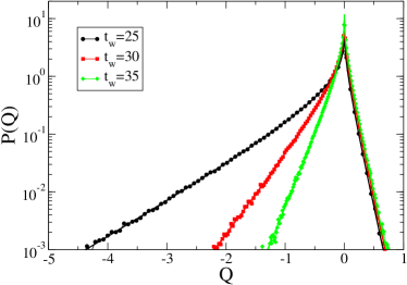
Figure 2: Heat probability distribution for the single oscillator, with $\omega=10^{-1}$, $T_{0}=100$ and $T=10^{-1}$, for $t=200$ and different values of $t_{w}$. Analytical form from Eq. (51) (continuous lines) and numerical simulations (symbols).

III.2 Decomposition into cooling and heating contributions

The two quantities $\lambda_{\pm}$ turn out to be the basic building blocks in all what follows. The physical meaning can be readily understood by rewriting $P(Q)$ as the convolution of the two distributions arising in the purely cooling and in the purely heating process. Defining

$$P_{\pm}(Q)=\sqrt{\pm i\lambda_{\pm}}\int_{-\infty}^{\infty}\frac{d\lambda}{2\pi}\frac{e^{-i\lambda Q}}{\sqrt{\lambda\pm i\lambda_{\pm}}}$$ (54)

and carrying out the integral, which involves only one of the branch points, one finds

$$P_{-}(Q)=\left\{\begin{array}[]{ll}\sqrt{\frac{\lambda_{-}}{\pi|Q|}}e^{\lambda_{-}Q},\;\;$for$\;\;Q<0,\\ 0,\;\;$for$\;\;Q>0,\end{array}\right.$$ (55)

and

$$P_{+}(Q)=\left\{\begin{array}[]{ll}\sqrt{\frac{\lambda_{+}}{\pi Q}}e^{-\lambda_{+}Q},\;\;$for$\;\;Q>0,\\ 0,\;\;$for$\;\;Q<0,\end{array}\right.$$ (56)

from which follows

$$\lambda_{\pm}=\pm\frac{1}{2\langle{\cal Q}\rangle_{\pm}},$$ (57)

where $\langle{\cal Q}\rangle_{\pm}$ are the average heats exchanged in the processes in which heat can only be absorbed or released. Then, the probability (44) can be rewritten as

$$P(Q)=\int_{-\infty}^{\min(0,Q)}dQ^{\prime}P_{+}(Q-Q^{\prime})P_{-}(Q^{\prime}),$$ (58)

which reproduces the result of Eq. (51) and the total average heat exchanged is clearly given by

$$\langle{\cal Q}\rangle = \langle{\cal Q}\rangle_{+}+\langle{\cal Q}\rangle_{-}$$ (59)

$$= \frac{1}{2}\left(\frac{1}{\lambda_{+}}-\frac{1}{\lambda_{-}}\right)=-\frac{b}{2}.$$

The physical conditions for $P(Q)=P_{-}(Q)$ or $P(Q)=P_{+}(Q)$ are obtained putting the oscillator in contact with the thermal reservoir at $T=0$, or by arranging a purely heating process with $T_{0}=0,T>0$ and $t_{w}=0$. In the first case, one has $T_{w}=T_{0}G^{2}_{w},a=0,b=(T_{w}-T_{t})$ from which follows, according to Eqs. (48) and (49), $\lambda_{+}=\infty,\lambda_{-}=(T_{w}-T_{t})^{-1}$, implying $P_{+}(Q)=\delta(Q)$ and, therefore, according to Eq. (55)

$$P(Q)=P_{-}(Q)=\left\{\begin{array}[]{ll}\sqrt{\frac{1}{\pi|Q|(T_{w}-T_{t})}}e^{Q/(T_{w}-T_{t})},\;\;$for$\;\;Q<0,\\ 0,\;\;$for$\;\;Q>0.\end{array}\right.$$ (60)

Similarly, in the second case, with $T_{0}=0$ and $t_{w}=0$, one has $T_{w}=0,a=0,b=-T_{t}$, which yield $\lambda_{+}=1/T_{t},\lambda_{-}=\infty$, implying $P_{-}(Q)=\delta(Q)$ and

$$P(Q)=P_{+}(Q)=\left\{\begin{array}[]{ll}\sqrt{\frac{\beta_{t}}{\pi Q}}e^{-\beta_{t}Q},\;\;$for$\;\;Q>0,\\ 0,\;\;$for$\;\;Q<0.\end{array}\right.$$ (61)

III.3 FT and time reversal symmetry breaking

In this subsection we discuss the symmetry properties of the heat distribution. From Eq. (51) follows immediately the FT in the standard form

$$\frac{P(-Q)}{P(Q)}=e^{-\Delta\beta Q}.$$ (62)

A similar result was derived in Ref. salazar16 with $t_{w}=0$ and $\Delta\beta=\beta_{0}-\beta$, while in Ref. gomez11 there appears $\Delta\beta=\beta_{w}-\beta_{t}$, which holds true only in the limit of large $\tau$ when the system is time decorrelated and $\beta_{t}\sim\beta$. Hence, as anticipated in section II, the AF is linear

$${\cal K}(Q)=\Delta\beta Q,$$ (63)

since the role of the initial probability $P_{0}$ now is played by $P(x,t_{w})$, which after Eqs. (35) and (38) yields

$$\ln\frac{P(x_{w},t_{w})}{P(x,t_{w})}=\beta_{w}{\cal Q}.$$ (64)

Here, we want to highlight the connection between the above result and the breaking of the time reversal symmetry, by adapting to the present context the approach of Gaspard Gaspard sketched in Section II. Taking for $\Omega$ the set of ordered pairs $\sigma=(x_{w},x)$, the time reversal symmetry operation is represented by the involution $\sigma^{*}=(x,x_{w})$ which exchanges the order of $x_{w}$ and $x$. The task is to rewrite the joint probability Eq. (III.1) in the form of Eq. (12), that is as the product of a $\mathbb{Z}_{2}$ symmetric factor $\mu_{0}(\sigma)$ times an exponential where there appears the heat ${\cal Q}$ in the role of the observable explicitly breaking the $\mathbb{Z}_{2}$ symmetry. In order to do this, let us first cast the joint probability Eq. (III.1) in the form

$$\mu(\sigma)=\frac{1}{Z}e^{-{\cal A}(\sigma)},$$ (65)

where the “action” ${\cal A}(\sigma)$ can be read out from Eq. (III.1) as

$${\cal A}(\sigma)=\frac{\beta\omega}{2(1-G^{2})}\left[x^{2}-2Gxx_{w}+G^{2}x_{w}^{2}\right]+\beta_{w}\frac{1}{2}\omega x_{w}^{2},$$ (66)

and the normalization factor is given by $Z=\sqrt{\frac{2\pi\beta\beta_{w}\omega^{2}}{(1-G^{2})}}$. Decomposing ${\cal A}(\sigma)$ into the sum of an even and an odd part

$${\cal A}(\sigma)={\cal E}(\sigma)+{\cal O}(\sigma),$$ (67)

with

$${\cal E}(\sigma) = \frac{1}{2}\left[{\cal A}(\sigma)+{\cal A}(\sigma^{*})\right]$$ (68)

$$= \frac{\beta\omega}{4(1-G^{2})}\left[(1+G^{2})x^{2}-4Gxx_{w}\right.$$

$$+ \left.(1+G^{2})x_{w}^{2}\right]+\beta_{w}\frac{1}{4}\omega(x^{2}+x_{w}^{2}),$$

and

$${\cal O}(\sigma)=\frac{1}{2}\left[{\cal A}(\sigma)-{\cal A}(\sigma^{*})\right]=-\frac{1}{2}\Delta\beta{\cal Q}(\sigma),$$ (69)

where ${\cal Q}(\sigma)$ is defined by Eq. (35), the form (12) of $\mu(\sigma)$ is obtained

$$\mu(\sigma)=\mu_{0}(\sigma)e^{\frac{1}{2}\Delta\beta{\cal Q}(\sigma)},$$ (70)

where

$$\mu_{0}(\sigma)=\frac{1}{Z}e^{-{\cal E}(\sigma)},$$ (71)

is $\mathbb{Z}_{2}$ invariant. Therefore, the invariance under time reversal in $\mu(\sigma)$ is explicitly broken by the exponential factor involving ${\cal Q}(\sigma)$ in Eq. (70). Once this is established, the FT in the form of Eq. (62) is recovered straightforwardly. The following remarks are in order:

1. the affinity $\Delta\beta$ driving the heat flow plays the role of the external field causing the explicit breaking of the $\mathbb{Z}_{2}$ invariance.

2. The $\mathbb{Z}_{2}$ invariant measure $\mu_{0}(\sigma)$ of Eq. (71) is not time translation invariant, as it could have been naively expected, since the action ${\cal E}(\sigma)$ in Eq. (68) depends both on $\tau$, through $G$, and on $t_{w}$, through $\beta_{w}$. Computing $P(Q)$ from Eq. (70) one has

   $$P(Q)=\sum_{\sigma}\mu(\sigma)\delta({\cal Q}-Q)=e^{\frac{1}{2}\Delta\beta Q}\sum_{\sigma}\mu_{0}(\sigma)\delta({\cal Q}-Q),$$ (72)

   and, comparing with Eq. (51), one obtains

   $$\sum_{\sigma}\mu_{0}(\sigma)\delta({\cal Q}-Q)=\frac{\sqrt{\lambda_{+}\lambda_{-}}}{\pi}K_{0}\left(\frac{\lambda_{+}+\lambda_{-}}{2}|Q|\right).$$ (73)

3. From Eq. (44) it is straightforward to derive the moment generating function

   $$\langle e^{\vartheta{\cal Q}}\rangle=\sqrt{\frac{\lambda_{+}\lambda_{-}}{(\vartheta+\lambda_{-})(\lambda_{+}-\vartheta)}},$$ (74)

   implying that the cumulant generating function $\psi(\vartheta)=\ln\langle e^{\vartheta{\cal Q}}\rangle$ satisfies the same symmetry

   $$\psi(\vartheta)=\psi(-\vartheta+\Delta\beta),$$ (75)

   which was found for a particle coupled to two thermostats at different temperatures Farago .

IV Two Brownian oscillators

Let us, next, see how the overall heat fluctuations are modified when there are internal degrees of freedom. We consider first the case of two uncoupled oscillators with frequencies $\omega_{1}$ and $\omega_{2}$ and, in the next section, we consider the limit of a large number of oscillators.

As before, initially the system is in equilibrium at the temperature $T_{0}$ and at the time $t=0$ is put in contact with the reservoir at the temperature $T$. Denoting by $Q_{1}$ and $Q_{2}$ the amounts of heat exchanged by each oscillator, the probability that the system as a whole exchanges the heat $Q$ is given by

$$P(Q)=\int_{-\infty}^{\infty}dQ_{1}\,P_{1}(Q_{1})P_{2}(Q-Q_{1}),$$ (76)

where $P_{i}(Q_{i})$, with $i=1,2$, are the probabilities pertaining to each component. Inserting the expression (51) and changing the integration variable from $Q_{1}$ to $y=Q_{1}-Q/2$, this can be put in the form analogous to Eq. (51)

$$P(Q)=e^{\frac{1}{2}\overline{\Delta\beta}Q}R(Q),$$ (77)

where

$$\overline{\Delta\beta}=\frac{1}{2}(\Delta\beta_{1}+\Delta\beta_{2}),$$ (78)

and

$$R(Q)=\int_{-\infty}^{\infty}dy\,W_{1}(y+Q/2)W_{2}(y-Q/2)e^{\frac{1}{2}(\Delta\beta_{1}-\Delta\beta_{2})y},$$ (79)

with

$$W_{i}(x)=\frac{\sqrt{\lambda_{+,i}\lambda_{-,i}}}{\pi}K_{0}\left(\frac{\lambda_{+,i}+\lambda_{-,i}}{2}|x|\right).$$ (80)

Here, $\lambda_{+,i}$ are defined in Eq. (45), the index $i=1,2$ denoting the oscillator frequencies, $\omega_{1}$ and $\omega_{2}$, respectively and $\Delta\beta_{i}$ is defined by Eqs. (39) and (52) with frequency $\omega_{i}$. The resulting AF is given by

$${\cal K}(Q)=\overline{\Delta\beta}Q+\ln\left(\frac{R(Q)}{R(-Q)}\right).$$ (81)

Hence, if the two oscillators are equal ($\omega_{1}=\omega_{2}$) the second term disappears, since $R(Q)$ becomes an even function, and the linear result (63) is recovered. If they are unequal, $R(Q)$ is not even under the change of sign of $Q$ and the second term in the above equation gives a nonlinear contribution. The modifications introduced by this second contribution are illustrated by Fig. 3 obtained with parameters $\omega_{1}=0.5$ and $\omega_{2}=0.2$, $T_{0}=10$, $T=1$ at times $t=12,t_{w}=10$. Around $Q=0$ one observes a linear behavior with slope $\overline{\Delta\beta}$ (see dashed line in the inset), while for large values of $Q$ the AF shows a nonmonotonic behavior.

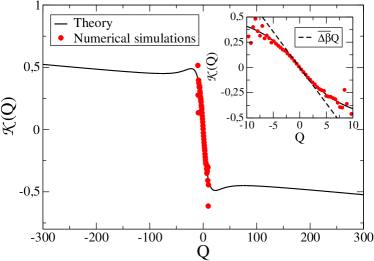
Figure 3: Asymmetry function for two Brownian oscillators with frequencies $\omega_{1}=0.5$ and $\omega_{2}=0.2$, for $T_{0}=10$, $T=1$, $t_{w}=10$ and $t_{w}=12$. The line represents the analytical expression Eq. (81), while the points are numerical simulations. In the inset a zoom of the region at small $Q$ is shown.

In order to expose the connection between the presence of internal structure and the equilibrium problem mentioned in the Introduction, let us go back to the microscopic measure. With two oscillators the phase space enlarges to the set of pairs $\Omega=\{\sigma_{1},\sigma_{2}\}$ and the corresponding action, due to the absence of coupling, is additive

$${\cal A}(\sigma_{1},\sigma_{2})={\cal A}_{1}(\sigma_{1})+{\cal A}_{2}(\sigma_{2}).$$ (82)

The two terms in the right hand side are given by Eq. (66), keeping into account that the frequencies $\omega_{1}$ and $\omega_{2}$ are different, that is

$${\cal A}_{i}(\sigma_{i}) = \frac{\beta\omega_{i}}{2(1-G_{i}^{2})}\left[x_{i}^{2}-2G_{i}x_{i}x_{w,i}+G_{i}^{2}x_{w,i}^{2}\right]$$ (83)

$$+ \beta_{w,i}\frac{1}{2}\omega_{i}x_{w,i}^{2}.$$

Carrying out the decomposition into even and odd parts, as in Eq. (67),

$${\cal A}(\sigma_{1},\sigma_{2})={\cal E}(\sigma_{1},\sigma_{2})+{\cal O}(\sigma_{1},\sigma_{2}),$$ (84)

the measure can be written as

$$\mu(\sigma_{1},\sigma_{2})=\mu_{0}(\sigma_{1},\sigma_{2})e^{-{\cal O}(\sigma_{1},\sigma_{2})},$$ (85)

where

$$\mu_{0}(\sigma_{1},\sigma_{2})=\frac{1}{Z}e^{-{\cal E}(\sigma_{1},\sigma_{2})},$$ (86)

is even under $*:(\sigma_{1},\sigma_{2})\mapsto(\sigma^{*}_{1},\sigma^{*}_{2})$, while

$${\cal O}(\sigma_{1},\sigma_{2})=-\frac{1}{2}[\Delta\beta_{1}{\cal Q}_{1}(\sigma_{1})+\Delta\beta_{2}{\cal Q}_{2}(\sigma_{2})]$$ (87)

is odd. Hence, ${\cal W}(\sigma_{1},\sigma_{2})=-2{\cal O}(\sigma_{1},\sigma_{2})$ and from Eq. (10) there follows

$$\frac{P(-Q)}{P(Q)}=e^{-{\cal K}(Q)},$$ (88)

with

$${\cal K}(Q)=-\ln\langle e^{-\sum_{i}\Delta\beta_{i}{\cal Q}_{i}}|{\cal Q}=Q\rangle.$$ (89)

The formal similarity with Eq. (14) is evident, with the affinities $\Delta\beta_{i}$ playing the role of the site dependent external field $\{B_{i}\}$ and the partial heat ${\cal Q}_{i}$ that of the local order parameter $s_{i}$. Accordingly, the above expression simplifies in the particular case akin to that of the uniform external field, that is for $\omega_{1}=\omega_{2}$ or for $t_{w}=0$, yielding $\Delta\beta_{i}=\beta_{0}-\beta$ for all $i$.

V Extended system

In this section we consider the case of a large number of oscillators. The aim is to analyse important qualitatively new features arising in the behavior of fluctuations when the size of the system becomes large. As it is usually the case for large systems, fluctuations of extensive quantities, such as heat, obey a large deviation principle hugo ; ld . The non trivial feature, unexpected for a linear system, is that in the large deviation function there appears a singularity corresponding to a condensation transition Gonnella ; Jo ; Pechino . This means, as briefly anticipated in the Introduction, that there exists a critical threshold $Q_{c}$ of the exchanged heat, such that fluctuations above threshold are due to a single oscillator. We give a careful treatment of the saddle point computation involved in the computation of the large deviation function and we study the phase diagram of the transition. Mathematical details are collected in Appendix A.

We consider an extended system of linear size $L$ and volume $V=L^{d}$, where $d$ is the space dimensionality. We suppose that this system is linear and that the normal modes decomposition with periodic boundary conditions gives rise to a set of harmonic components for the low lying modes with frequencies obeying the dispersion relation note

$$\omega(\mathbf{k})=k^{\alpha}+\omega_{0},$$ (90)

where $\omega_{0}>0$, $\mathbf{k}=\frac{2\pi}{L}\mathbf{n},\,\,n_{i}=0,\pm 1,\pm 2,...$ and $\alpha>0$. Just to fix ideas, a dispersion relation of this type arises in the Gaussian model or Van Hove theory of critical phenomena Ma . The $\mathbf{k}$-space volume per mode is $(2\pi)^{d}/V$. Assuming that there exists an underlying lattice structure with lattice spacing $a_{0}$, the first Brillouin zone is bounded by $\Lambda=2\pi/a_{0}$ and the total number of modes is given by $N=V/a_{0}^{d}$. Due to modes independence, the probability of a generic microscopic state at the time $t_{w}$ is given by the product measure

$$P(\{x_{\mathbf{k}}\},t_{w})=\prod_{\mathbf{k}}\sqrt{\frac{\beta_{\mathbf{k},w}\omega(\mathbf{k})}{2\pi}}e^{-\beta_{\mathbf{k},w}{\cal H}_{\mathbf{k}}(x_{\mathbf{k}})},$$ (91)

where, according to Eq. (40),

$$\beta_{\mathbf{k},w}=[(T_{0}-T)e^{-2\omega(\mathbf{k})t_{w}}+T]^{-1}.$$ (92)

is the inverse effective temperature of the mode $\mathbf{k}$ and ${\cal H}_{\mathbf{k}}(x_{\mathbf{k}})=(1/2)\omega(\mathbf{k})x^{2}_{\mathbf{k}}$ is the single mode energy. Hence, Eq. (64) generalizes to

$$\frac{P(\{x_{\mathbf{k}}\},t_{w})}{P(\{x_{\mathbf{k},w}\},t_{w})}=e^{-\sum_{\mathbf{k}}\beta_{\mathbf{k},w}{\cal Q}_{\mathbf{k}}},$$ (93)

where ${\cal Q}_{\mathbf{k}}={\cal H}_{\mathbf{k}}(x_{\mathbf{k}})-{\cal H}_{\mathbf{k}}(x_{\mathbf{k},w})$ is the heat exchanged by the mode $\mathbf{k}$, and the sum is restricted to the first Brillouin zone. Inserting into Eq. (29) we recover Eq. (30)

$${\cal K}(Q)=-\ln\bigl{\langle}e^{-\sum_{\mathbf{k}}\Delta\beta_{\mathbf{k}}{\cal Q}_{\mathbf{k}}}|{\cal Q}=Q\bigr{\rangle}.$$ (94)

Comparing with Eq. (14), we see that the differences $\Delta\beta_{\mathbf{k}}=\beta_{\mathbf{k},w}-\beta$ play the role of the site dependent external field in the equilibrium problem, as remarked in section IV, and that the AF linear form is recovered when these differences become independent of $\mathbf{k}$, as for instance for $t_{w}=0$, or when the oscillators are identical, i.e. $\alpha=0$ (see Appendix B).

Let us, next, see what form takes the AF by letting $N$ to become large. Generalizing Eq. (76) and keeping $V$ finite, the probability that the system exchanges the amount of heat $Q$ is given by

$$P(Q,V)=\int_{-\infty}^{\infty}\prod_{\mathbf{k}}dQ_{\mathbf{k}}\,P_{\mathbf{k}}(Q_{\mathbf{k}})\,\delta(Q-\sum_{\mathbf{k}}Q_{\mathbf{k}})$$

$$= \int_{-i\infty}^{i\infty}\frac{d\lambda}{2\pi i}\,e^{-\lambda Q}\prod_{\mathbf{k}}\sqrt{\frac{\lambda_{+}(k)\lambda_{-}(k)}{[\lambda_{+}(k)-\lambda][\lambda_{-}(k)+\lambda]}},$$

where $\lambda_{\pm}(k)$ are defined in Eq. (45), evaluated for $\omega(\mathbf{k})$ as in Eq. (90). Denoting by $\lambda^{+}_{0}$ and $\lambda^{-}_{0}$ the upper and lower edges of the two branches of the spectrum, that is

$$\lambda^{+}_{0}=\min_{0\leq k\leq\Lambda}\{\lambda_{+}(k)\},\,\,\,\lambda^{-}_{0}=\min_{0\leq k\leq\Lambda}\{\lambda_{-}(k)\},$$ (96)

the contour of integration can be deformed to an arbitrary line $\Gamma$ on the complex plane, provided it crosses the real axis within the gap $[-\lambda^{-}_{0},\lambda^{+}_{0}]$. This allows to rewrite the above integral as

$$P(Q,V)=\int_{\Gamma}\frac{dz}{2\pi i}\,e^{-V[zq+L(z;V)]},$$ (97)

where $q=Q/V$ is the density of the exchanged heat and

$$L(z;V)=\frac{1}{2V}\sum_{0\leq\mathbf{k}\leq\Lambda}\ln\left[\frac{[\lambda_{+}(k)-z][z+\lambda_{-}(k)]}{\lambda_{+}(k)\lambda_{-}(k)}\right].$$ (98)

The large $V$ behavior of $P(Q,V)$ can be obtained by using the steepest descent method to estimate the integral in Eq. (97) nota . When $V\gg 1$ the wave vector $\mathbf{k}$ can be assumed continuous and the sum in Eq. (98) approximated by an integral with an error of $O(1/V)$. The neglected $O(1/V)$ terms in the exponent, however, give an $O(1)$ contribution to $P(Q;V)$, resulting in an undetermined normalization of $P(Q;V)$, memory of the discrete nature of $\mathbf{k}$.

The function $L(z;V)$ contains the dangerous boundary terms $(1/V)\ln[\lambda_{0}^{+}-z]$ and $(1/V)\ln[\lambda_{0}^{-}+z]$. If the steepest descent path $\Gamma$ does not come too close to either edges $z=\pm\lambda_{0}^{\pm}$ of the gap these terms just give an $O(1/V)$ correction which can be included into the normalization factor. Consequently, in this case the function

$$L(z)=\frac{1}{2}\int_{0}^{\Lambda}d\mu(k)\,\ln\left[\frac{[\lambda_{+}(k)-z][z+\lambda_{-}(k)]}{\lambda_{+}(k)\lambda_{-}(k)}\right],$$ (99)

with $d\mu(k)=\Upsilon_{d}k^{d-1}dk$ and $\Upsilon_{d}=[2^{d-1}\pi^{d/2}\Gamma(d/2)]^{-1}$ coming from the angular integration, is an uniform approximation to the function $L(z;V)$ as $V\gg 1$. Here, $\Gamma(x)$ denotes the Euler gamma function.

Denoting by $\phi(z;q)=zq+L(z)$ and by primes derivatives with respect to $z$, it is straightforward to verify that $\mathbb{I}m\,\phi^{\prime}(z;q)\sim\mathbb{I}m\,z$, implying that the stationary point $z^{*}$ of $\phi(z;q)$ is on the real axis. Thus, setting $z=x+iy$, the coordinate $x^{*}$ of the saddle point is obtained solving the equation $\phi^{\prime}(x^{*};q)=0$, which explicitly reads

$$q = -L^{\prime}(x^{*})$$ (100)

$$= \frac{1}{2}\int_{0}^{\Lambda}d\mu(k)\,\left[\frac{1}{\lambda_{+}(k)-x^{*}}-\frac{1}{\lambda_{-}(k)+x^{*}}\right].$$

The function $-L^{\prime}(x)$ is monotonically increasing in the interval $x\in[-\lambda_{0}^{-},\lambda_{0}^{+}]$, so Eq. (100) admits solution on the condition that $q$ lies between the limiting values:

$$q_{c}^{\pm}=-L^{\prime}(\pm\lambda_{0}^{\pm}),$$ (101)

with $q_{c}^{-}<0<q_{c}^{+}$. In this case the steepest descent path in the neighborhood of the saddle point is parallel to the imaginary axis and a straightforward calculation leads to the asymptotic result for $V\gg 1$

$$P(Q,V)=\frac{1}{\sqrt{-2\pi VL^{\prime\prime}(x^{*})}}\,e^{-V[qx^{*}+L(x^{*})]}.$$ (102)

If both $q_{c}^{\pm}$ diverge this result is valid for arbitrary finite values of $q$ because $x^{*}$ is always inside the gap $[-\lambda^{-}_{0},\lambda^{+}_{0}]$, and far from the edges. If, instead, one or both $q_{c}^{\pm}$ are finite, the saddle point $x^{*}$ may reach the boundary of the gap $[-\lambda^{-}_{0},\lambda^{+}_{0}]$, and leave it for $q<q_{c}^{-}$ or $q>q_{c}^{+}$. When this occurs the asymptotic approximation in Eq. (102) is no more valid.

The boundary values $q_{c}^{\pm}$ are finite or infinite depending on whether the singularities of the integrand function in $L^{\prime}(x)$ are integrable or not. More specifically, let us denote by $k^{\pm}_{0}$ the wave vectors at which $\lambda_{\pm}(k)$ attain the minimum value, that is $\lambda_{\pm}(k^{\pm}_{0})=\lambda^{\pm}_{0}$. Then, in the neighborhoods of $k^{\pm}_{0}$,

$$\lambda_{{\pm}}(k)-\lambda^{\pm}_{0}\sim\begin{cases}C\,(k-k^{\pm}_{0})^{2n},&\text{for}\ k^{\pm}_{0}>0;\\ C\,k^{\alpha},&\text{for}\ k^{\pm}_{0}=0,\end{cases}$$ (103)

where $C$ is a positive constant, $n=1,2,\dotsc$ and $\alpha>0$. Therefore, $q_{c}^{\pm}$ diverge if $k^{\pm}_{0}>0$ or if $k^{\pm}_{0}=0$ and $d\leq\alpha$, while they are finite if $k^{\pm}_{0}=0$ and $d>\alpha$. Which is the case depends on the parameters of the quench $T_{0},T,\tau,t_{w}$. So, in general, this manifold of parameters is partitioned into phases distinguished by $q_{c}^{\pm}$ being finite or infinite.

For what follows, and before discussing how the steepest descent calculation must be modified, it is useful to get some insight into the meaning of the two different cases. Recalling that $\lambda_{+}(k)$ and $-\lambda_{-}(k)$ are the inverse average heat absorbed or released, it is evident from Eq. (100) that if $q$ coincides with the average heat density $\langle q\rangle$, then $x^{*}(\langle q\rangle)=0$, implying $-L^{\prime}(0)=\langle q\rangle$. Consequently, if $q$ differs from $\langle q\rangle$ then $x^{*}(q)\neq 0$ and

$$\lambda^{*}_{\pm}(k,q)=\lambda_{\pm}(k)\mp x^{*}(q)$$ (104)

acquire the meaning of the inverse average heat absorbed or released in new conditions, such that $q$ would be the new average total heat density, exactly as the $\{B_{i}^{*}\}$ of section II have been recognized to be the shifted external fields necessary to render the fluctuation $m$ equal to the average magnetization per spin. In other words, a deviation of $q$ from the average $\langle q\rangle$ brings in a shift by $x^{*}(q)$ of the inverse heats exchanged by the single modes. Accordingly, when $x^{*}(q)$ approaches the edges of the gap the above defined $\lambda_{0}^{\pm*}$ vanish, which means that the corresponding edge modes give an infinite contribution to the exchanged heat. This may happen either because the fluctuation $q$ itself is infinite, or because the contributions of all the modes, other than the edge ones, can sum up at most to the finite amounts $q_{c}^{\pm}$. In the latter case, if $|q|$ goes above the thresholds $|q_{c}^{\pm}|$, in order to make up for the finite difference $|q|-|q_{c}^{\pm}|$ a spike contribution must come from the edge modes at $k_{0}^{\pm}$. This phenomenon is the condensation of fluctuations in the edge mode, since as anticipated in the Introduction and at the beginning of this section, the entire amount of the fluctuation above the critical threshold comes from a single degree of freedom. The mechanism of the transition can be recognized to be the same as that of Bose-Eintein condensation Huang . More in general, condensation of fluctuations has been found in widely different contexts such as information theory Merhav , finance Filiasi and statistical mechanics encompassing both equilibirum and out of equilibrium situations JoEPL .

When one or both $q_{c}^{\pm}$ are finite, the steepest descent calculation must be modified. This case will be dealt with in the next subsection. Returning to the case in which Eq. (102) holds, neglecting subdominant terms and taking the ratio $P(-Q)/P(Q)$, one obtains the following explicit form of the AF

$$\frac{1}{V}{\cal K}(Q)=-[x^{*}(-q)+x^{*}(q)]q+[L(x^{*}(-q))-L(x^{*}(q))],$$ (105)

which is clearly reminiscent of Eq. (LABEL:G.5) in sect. II. In order to expose the analogy, let us subtract equations (104) one from the other and take the average over $k$, obtaining

$$x^{*}(q)=\frac{1}{2}\left(\overline{\lambda_{+}}-\overline{\lambda_{-}}\right)+\frac{1}{2}\left[\overline{\lambda_{-}^{*}(q)}-\overline{\lambda_{+}^{*}(q)}\right],$$ (106)

where

$$\overline{\lambda_{\pm}}=\frac{1}{{\cal N}}\int_{0}^{\Lambda}d\mu(k)\,\lambda_{\pm}(k),\,\,\,{\cal N}=\int_{0}^{\Lambda}d\mu(k)\,1,$$ (107)

and similar expressions for $\overline{\lambda_{\pm}^{*}(q)}$. Inserting into Eq. (105), we obtain

$$\frac{1}{V}{\cal K}(Q)=\left(\overline{\lambda_{-}}-\overline{\lambda_{+}}\right)q+\left[\Psi(-q)-\Psi(q)\right],$$ (108)

where

$$\Psi(q)=L(x^{*}(q))+\frac{1}{2}\left[\overline{\lambda_{-}^{*}(q)}-\overline{\lambda_{+}^{*}(q)}\right]q.$$ (109)

Hence, comparing with Eqs. (24) and (81), we can recognize the same structure: the prefactor $\left(\overline{\lambda_{-}}-\overline{\lambda_{+}}\right)$ of the linear contribution (the same appearing in the single oscillator case) plays the role of the external average field $\mathbb{B}$, while the nonlinear term $\left[\Psi(-q)-\Psi(q)\right]$, arises from “free energy” contributions. As remarked above, the presence of this latter term is due to the $k$-dependence of $\Delta\beta_{k}$, which plays the same role as the $i$-dependence of $B_{i}$.

V.1 Condensation transition

On physical grounds one can argue that condensation at finite $q_{c}^{-}$ can occur only in cooling experiments, where the final temperature is lower than the initial one, while condensation at finite $q_{c}^{+}$ can occur only in heating experiment. We do not have a proof of this, but numerical analysis of the conditions for condensation confirm this conjecture.

Let us thus concentrate on the case with $q_{c}^{+}=\infty$ and $q_{c}^{-}$ finite, which occurs for $k_{0}^{-}=0$ and $d>\alpha$. The analysis of the opposite case in which $q_{c}^{+}$ is finite and $q_{c}^{-}=-\infty$, (or both finite, if such a case exists) is straightforward.

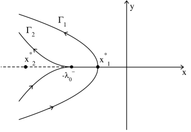
Figure 4: Schematic representation of the steepest descent path of integration. If $x^{*}=x_{1}^{*}\geq-\lambda_{0}^{-}$, the integration contour goes through $x_{1}^{*}$, where $\phi^{\prime}=0$, ($\Gamma_{1}$ curve). If $x^{*}=x_{2}^{*}<-\lambda_{0}^{-}$, the integration contour develops a cusp and sticks to $-\lambda_{0}^{-}$, ($\Gamma_{2}$ curve).

When $q_{c}^{-}$ is finite, Eq. (100) does not admit a solution with $x^{*}\in[-\lambda_{0}^{-},\lambda_{0}^{+}]$ whenever $q<q_{c}^{-}$. The problem is well known from the theory of Bose-Einstein condensation of an ideal gas of bosons Huang or from the “sticking” of the saddle point to a singularity in the solution of the spherical model of ferromagnetism Berlin . It arises because when $q<q_{c}^{-}=-L^{\prime}(\lambda_{0}^{-})$ the steepest descent path cannot pass through the stationary point $x^{*}<-\lambda_{0}^{-}$ of $\phi(z;q)=zq+L(z)$ and must traverse the real axis at the gap edge $z=-\lambda_{0}^{-}$. Since $\phi^{\prime}(-\lambda_{0}^{-};q)=q-q_{c}^{-}$ is negative for $q<q_{c}^{-}$, the steepest descent path at $z=-\lambda_{0}^{-}$ bends toward the negative real axis forming the cusp characteristic of saddle point sticking at the gap edge (see Fig. 4). The large $V$ behavior of $P(Q,V)$ is dominated by the neighborhood of the gap edge because $\phi(-\lambda_{0}^{-};q)<\phi(x^{*};q)$ leading to the asymptotic behavior for $V\gg 1$:

$$P(Q,V)=\frac{1}{\sqrt{-\pi V\bigl{(}q-q_{c}^{-}\bigr{)}}}\,e^{-V[-\lambda_{0}^{-}q+L(-\lambda_{0}^{-})]},$$ (110)

valid for $q<q_{c}^{-}$.

As a matter of fact, this expression and Eq. (102) valid for $q>q_{c}^{-}$, hold for $x^{*}$ not to close to the gap edge $-\lambda_{0}^{-}$. That is, respectively, in the condensed phase and normal phase for $q$ not too close to $q_{c}^{-}$. The analysis of the asymptotic behavior of $P(Q,V)$ as $V\gg 1$ for all values of $q$, including close to $q_{c}^{-}$, requires some care. Details can be found in Appendix A.

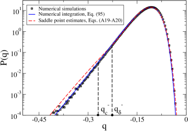
Figure 5: Comparison of the saddle point computation of $P(q)$ with the numerical computation of the same quantity for $\omega_{0}=0.1$, $T_{0}=100$, $T=0.1$, $t_{w}=3$, $\tau=7$, for a system with $L=41$ in $d=2$ ($N=1681$ oscillators), and with $\alpha=1$. (The quantity $q_{\delta}^{-}$ is defined in Eq. (120)).

Adding and subtracting $\lambda_{0}^{-}q_{c}^{-}$ in the exponent of Eq. (110), $P(Q;V)$ in the condensed phase far from the critical point can be written as

$$P(Q,V)=\frac{e^{\lambda_{0}^{-}(Q-Q_{c}^{-})}}{\sqrt{\pi\bigl{|}Q-Q_{c}^{-}\bigr{|}}}\,e^{V[\lambda_{0}^{-}q_{c}^{-}-L(-\lambda_{0}^{-})]},$$ (111)

where $Q_{c}^{-}=Vq_{c}^{-}$. Comparing the first term with the expression (55) for the distribution in the purely cooling process we have

$$P(Q,V)=P_{k=0,-}(Q-Q^{-}_{c})\,P(Q^{-}_{c},V),$$ (112)

where, up to normalization factors,

$$P(Q_{c}^{-},V)\sim e^{V[\lambda_{0}^{-}q_{c}^{-}-L(-\lambda_{0}^{-})]}.$$ (113)

This means that negative fluctuations below the critical lower threshold $Q^{-}_{c}$ condense into the cooling contribution of the $\mathbf{k}=0$ mode for the exceeding part $(Q-Q^{-}_{c})$, while the contribution of all the other modes is locked onto $Q^{-}_{c}$. The comparison of the saddle point estimates of $P(Q,V)$, in the normal and in the condensed phase, with the “exact” numerical computation is illustrated in Fig. 5.

V.2 Phase diagram

In order to establish the “phase” structure, it is necessary to analyse the behavior of $k^{\pm}_{0}>0$. Let us first recall the results of Ref. Pechino , where the problem was analysed for the quench to $T=0$. This is the simplest case because, as specified in section III.2, heat can only be released and we have to deal only with the $\lambda_{-}(k)$ branch of the spectrum. Differentiating with respect to $k$ the expression for $\lambda_{-}(k)$, given by the first line of Eq. (49), we get

$$\frac{\partial\lambda_{-}}{\partial k}=C(k,\tau,t_{w})A(k,\tau,t_{w}),$$ (114)

where $C(k,\tau,t_{w})=b^{-2}\Delta Te^{-2\omega(\vec{k})(t_{w}+\tau)}\alpha k^{\alpha-1}$ is a positive quantity, while

$$A(k,\tau,t_{w})=t_{w}e^{2\omega(\vec{k})\tau}[1-e^{2(E-k^{\alpha})\tau}],$$ (115)

has the sign of $(k^{\alpha}-E)$, with

$$E(\tau,t_{w})=\frac{1}{2\tau}\ln\left(1+\frac{\tau}{t_{w}}\right)-\omega_{0},$$ (116)

and vanishes at $k^{\alpha}=E$. Therefore, imposing the condition $E(\tau,t_{w})=0$, in the $(\tau,t_{w})$ plane there remains defined the critical line, given by

$$t_{w}=\frac{\tau}{e^{2\omega_{0}\tau}-1},$$ (117)

such that above it $k_{0}^{-}=0$, while below $k_{0}^{-}>0$. Thus, $k_{0}^{-}$ or, equivalently, $q_{c}^{-}$ act as order parameters and below the critical line the system is in the normal phase, corresponding to $q_{c}^{-}=-\infty$, while above it is in the condensed phase, corresponding to $q_{c}^{-}$ finite, as illustrated in Fig. 6 (black line).

If $T>0$, we must take into account both branches $\lambda_{\pm}(k)$ and keep track of the two order parameters $q_{c}^{\pm}$. The analytical search of the critical lines turns out to be quite complicated. So, we have looked for the absolute minima of $\lambda_{\pm}(k)$ numerically. The resulting phase diagram for $q_{c}^{-}$ is depicted in Fig. 6 for a few values of $T$, ranging from very low to almost equal to $T_{0}$. When the system is equilibrated ($T=T_{0}$), there is no condensed phase. Fig. 6 shows that upon lowering $T$ there appears a condensed phase which, starting from the far right, pronges toward the left eventually filling the entire region above the $T=0$ critical line. The prominent qualitative difference between the $T=0$ and the $T>0$ phase diagrams for $q_{c}^{-}$ is that in the latter case the transition driven by an increasing $t_{w}$, for fixed $\tau$, manifests reentrant behavior. The same computation for $q_{c}^{+}$ does not show the existence of a condensed phase, namely $q_{c}^{+}=\infty$ all over the explored $(\tau,t_{w})$ plane.

The reentrant behavior of the phase diagram can be interpreted as follows. Let us consider a quench at finite temperature, and let us fix $\tau$. Then, for small enough $t_{w}$, all oscillators are out of equilibrium and can exchange an arbitrary amount of heat with the bath. Therefore no condensation can take place in this region. Upon increasing $t_{w}$, all oscillators do equilibrate but the slowest one, corresponding to the mode $k=0$, that can account for large exchange of heat (above the threshold), leading to the condensation of fluctuations. Eventually, for large $t_{w}$, all oscillators are equilibrated and again the normal phase is recovered.

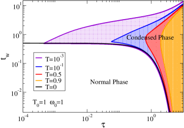
Figure 6: $q_{c}^{-}$ phase diagram for various final temperatures $T$ and for $T_{0}=1$. The normal phase corresponds to $q_{c}^{-}=\infty$, while the condensed phase to $q_{c}^{-}$ finite.

VI Conclusions

In this paper we have studied the fluctuations of the heat exchanged with the environment by a system of oscillators relaxing after a temperature quench. Focusing on the FT, we have investigated the relation between the deviations from linearity of the AF and the internal structure of the system, building on the analogy with the behavior of fluctuations in equilibrium when a symmetry is broken by nonuniform external perturbations.

We have first analysed in great detail the case of a single oscillator, reducing it to the convolution of the two elementary processes in which heat can be only released or only absorbed. The inverse average heats released $(\lambda_{-})$ and absorbed $(\lambda_{+})$ in these processes turn out to be the basic objects underlying the behavior of the quantities of interest. In the one-oscillator case the AF is linear with slope given by the difference $\Delta\beta=\lambda_{-}-\lambda_{+}$ and, in the framework of the above mentioned analogy with the equilibrium problem, this quantity acts like an external field explicitly breaking the time reversal symmetry. By adding a second oscillator it starts to surface the role of the dishomogeneity of the external perturbation in determining deviations from linearity in the AF. It should be pointed out that in the dynamical problem the lack of homogeneity is due to the existence of different relaxation rates, related to the presence of degrees of freedom evolving on different time scales. This produces a temporal dishomogeneity, which induces a differentiation of the affinities $\Delta\beta_{1}$ and $\Delta\beta_{2}$, analogous to the spatial heterogeneity generated by the external field $\{B_{i}\}$.

This picture emerges most clearly in the case of a large number of oscillators. In this case, the system, although diagonal, presents nontrivial features, the most notable of which is the possible condensation of fluctuations Gonnella ; Jo ; Pechino . Here, we have presented a detailed analytical study of the large deviation function of the heat distribution, with an accurate treatment of the crossover from the normal to the condensed phase, pointing out some interesting technical points involved in the application of the steepest descent method in the presence of a transition. In addition, we have mapped out the phase diagram of the condensation transition, discovering an unexpected reentrant behavior, in the $(t_{w},\tau)$ plane.

Our analysis allowed us to establish a close correspondence with the structure of the AF for the paramagnet in equilibrium under the action of a nonuniform external field. In the equilibrium case it seems reasonable to make the statement that the linearity of the AF depends on whether the observable of interest ${\cal M}(\sigma)$ is conjugate to the external perturbation, the implication of which being that deviations from the FT are due to the lack of conjugation. Clearly, the interesting and challenging issue is to understand whether this way of looking at the AF and its deviations from linearity can be extended to the nonequilibrium case. The study we have presented in this paper is a first step in this direction, paving the way to futures investigations within the context of more complex interacting systems, showing slow relaxation and aging phenomena.

Appendix A

In this Appendix we derive the uniform asymptotic expansions of $P(Q,V)$ as $V\gg 1$ valid for all values of $q=Q/V$, including at the condensation transition. As in the main text we shall assume $q_{c}^{+}=\infty$ and $q_{c}^{-}$ finite so that the steepest descent path hits the gap lower edge at the finite value $q=q_{c}^{-}$. Close to the edge $z=-\lambda_{0}^{-}$ the dangerous boundary term $(1/V)\ln[\lambda_{0}^{-}+z]$ is no more negligible, thus the uniform approximation $L(z)$, Eq. (99), to $L(z;V)$ as $V\gg 1$ breaks up and shuld be replaced by

$$L(z;V)=\frac{1}{2V}\ln\bigl{[}\lambda_{0}^{-}+z\bigr{]}+L(z)+O(1/V).$$ (118)

However, the function $L(z)$ is nonanalytic at $z=-\lambda_{0}^{-}$ while $L(z;V)-\frac{1}{2V}\ln\bigl{[}\lambda_{0}^{-}+z\bigr{]}$ is regular at the gap edge $-\lambda_{0}^{-}$, see Eq. (98). Therefore, to construct an uniform asymptotic approximation to $P(Q;V)$ as $V\gg 1$ valid for all values of $q$ the function $L(z)$ must be regularised. Hence, in Eq. (118) the function $L(z)$ is replaced by

$$\begin{split}L_{\delta}(z)&=\frac{1}{2}\int_{\delta}^{\Lambda}d\mu(k)\ln\left[\frac{\lambda_{-}(k)+z}{\lambda_{-}(k)}\right]\\ &\phantom{====}+\frac{1}{2}\int_{0}^{\Lambda}d\mu(k)\ln\left[\frac{\lambda_{+}(k)-z}{\lambda_{+}(k)}\right],\end{split}$$ (119)

where $\delta=O(1/V^{1/d})$ is an infrared cut-off Note2 . Without loss of generality we can take $\delta=V^{-1/d}$ because any proportionality constant can be absorbed into the $O(1/V)$ corrections in Eq. (118). Notice that the boundary value of $q$ separating the two phases becomes:

$$q_{\delta}^{-}=-L_{\delta}^{\prime}(-\lambda_{0}^{-}).$$ (120)

Using $\lambda_{+}(k)-\lambda_{0}^{-}\sim Ck^{\alpha}$ as $k\ll 1$, the finite volume correction to the critical point reads in the large $V$ limit:

$$q_{\delta}^{-}=q_{c}^{-}+\frac{\Upsilon_{d}}{2C(d-\alpha)}V^{\alpha/d-1}+o(V^{\alpha/d-1}),$$ (121)

where $\Upsilon_{d}=[2^{d-1}\pi^{d/2}\Gamma(d/2)]^{-1}$ and $\Gamma(x)$ is the Euler’s gamma function.

Replacing $L(z;V)$ into Eq. (97), neglecting the contribution from the $O(1/V)$ terms and taking $z=-\lambda_{0}^{-}+t$ to move the end point of the cut $(-\infty;-\lambda_{0}^{-}]$ on the negative real axis to $t=0$, leads to:

$$P(Q,V)=\int_{\Gamma}\frac{dt}{2\pi i}\,t^{-1/2}\,e^{-V\phi(-\lambda_{0}^{-}+t;q)},$$ (122)

where $\phi(z;q)=zq+L_{\delta}(z)$. As discussed in the main text, the stationary point $t^{*}$ of $\phi(-\lambda_{0}^{-}+t;q)$, solution of $\phi^{\prime}(-\lambda_{0}^{-}+t^{*};q)=q+L_{\delta}^{\prime}(-\lambda_{0}^{-}+t^{*})=0$ is on the real axis. The function $\phi(-\lambda_{0}^{-}+t;q)$ is analytic at $t=0$ and

$$\phi_{\delta}^{\prime}(-\lambda_{0}^{-};q)=q+L_{\delta}^{\prime}(-\lambda_{0}^{-})=q-q_{\delta}^{-}$$ (123)

changes sign at $q=q_{\delta}^{-}$, and is negative if $q<q_{\delta}^{-}$ and positive if $q>q_{\delta}^{-}$.

Far from the critical point, i.e., $|q-q_{\delta}^{-}|=O(1)$ as $V\gg 1$, the steepest descent calculation is straightforward. If $q>q_{\delta}^{-}$ the saddle point lies on the positive $t$-axis and the steepest descent path can pass through it. Near $t^{*}$ the steepest descent path is parallel to the imaginary axis and

$$P_{\rm out}(Q,V)=\frac{e^{-V\phi(-\lambda_{0}^{-}+t^{*};q)}}{\sqrt{-2\pi Vt^{*}L_{\delta}^{\prime\prime}(-\lambda_{0}^{-}+t^{*})}},$$ (124)

as $V\gg 1$, cfr. Eq. (102). In the opposite case $q<q_{\delta}^{-}$ the stationary point $t^{*}$ is negative and the steepest descent path cannot pass through it. Thus it must traverse the real axis at the gap edge $t=0$. Since $\phi_{\delta}^{\prime}(-\lambda_{0}^{-};q)$ is negative for $q<q_{\delta}^{-}$, the steepest descent path bends toward the negative real axis at $t=0$ forming the cusp characteristic of saddle point sticking at the gap edge (see Fig. 4). The asymptotic behavior for $V\gg 1$ is dominated by the gap edge because $\phi(-\lambda_{0}^{-};q)<\phi(-\lambda_{0}^{-}+t^{*};q)$. In the neighborhood of $t=0$ the steepest descent path is parallel to the negative real axis, hence using (123),

$$P_{\rm out}(Q,V)=\frac{e^{-V\phi(-\lambda_{0}^{-};q)}}{\sqrt{-\pi V\bigl{(}q-q_{\delta}^{-}\bigr{)}}},$$ (125)

as $V\gg 1$, cfr. Eq. (110).

When $|q-q_{\delta}^{-}|\ll 1$ as $V\gg 1$, $q$ is very close to $q_{\delta}^{-}$ and the stationary point is at $|t^{*}|\ll 1$. In this region we can expand $\phi(-\lambda_{0}^{-}+t;q)$ in powers of $t$:

$$\phi(-\lambda_{0}^{-}+t;q)=\phi_{0}+\phi_{0}^{\prime}\,t+\frac{1}{2}\phi_{0}^{\prime\prime}\,t^{2}+O(t^{3}),\quad|t|\ll 1,$$ (126)

where $\phi_{0}^{(n)}=\phi^{(n)}(-\lambda_{0}^{-};q)$. The first three terms of the expansion must be retained; subsequent terms just give corrections to the leading asymptotic expansion and can be neglected.

Using the expansion (126) the stationary point is at:

$$\phi^{\prime}(-\lambda_{0}^{-}+t^{*};q)=0\ \Rightarrow\ t^{*}=-\frac{\phi_{0}^{\prime}}{\phi_{0}^{\prime\prime}}=-\frac{q-q_{\delta}^{-}}{L_{\delta}(-\lambda_{0}^{-})}.$$ (127)

Consider first the case $\phi_{0}^{\prime}>0$, that is $q>q_{\delta}^{-}$. In this case $t^{*}>0$, because $L_{\delta}^{\prime\prime}(-\lambda_{0}^{-})<0$, and the steepest descent path can go through the saddle point at $t^{*}$. Thus, expanding Eq. (126) around $t^{*}$ and inserting the results into Eq. (122) leads to:

$$P_{\rm in}(Q,V)={\mathcal{N}}_{+}(q)\,\exp\left[-V\left(\phi_{0}-\frac{\phi_{0}^{\prime 2}}{2\phi_{0}^{\prime\prime}}\right)\right]$$ (128)

where

$${\mathcal{N}}_{+}(q)=\int_{\Gamma}\frac{dt}{2\pi i}\,t^{-1/2}\,e^{\frac{V}{2}|\phi_{0}^{\prime\prime}|(t-t^{*})^{2}}.$$ (129)

The steepest descent path is the vertical line $\mathbb{R}e\,(t-t^{*})=0$ passing at $t^{*}$. Inside the critical region $|\phi_{0}^{\prime\prime}|(t-t^{*})^{2}=O(1/V)$ as $V\gg 1$, so the steepest descent path is given by $t-t^{*}=iy/\sqrt{V|\phi_{0}^{\prime\prime}|}$. Introducing the variable

$$\xi=\sqrt{V|\phi_{0}^{\prime\prime}|}\,t^{*}=\sqrt{\frac{V}{|\phi_{0}^{\prime\prime}|}}\,\phi_{0}^{\prime},$$ (130)

Eq. (129) becomes:

$${\mathcal{N}}_{+}(\xi)=\frac{1}{[V|\phi_{0}^{\prime\prime}|]^{1/4}}\int_{-\infty}^{+\infty}\frac{dy}{2\pi}\,(\xi+iy)^{-1/2}e^{-y^{2}/2}.\\$$ (131)

To evaluate the integral we shift the integration axis vertically by $i\xi$. The singularity $(\xi+iy)^{-1/2}$ at $y=i\xi$ gives no contribution, so we have

$${\mathcal{N}}_{+}(\xi) =\frac{1}{2\pi}\frac{e^{\xi^{2}/2}}{[V|\phi_{0}^{\prime\prime}|]^{1/4}}\int_{-\infty}^{+\infty}dy\,(iy)^{-1/2}e^{-y^{2}/2-i\xi y}$$

$$=\frac{1}{\sqrt{2\pi}}\frac{e^{\xi^{2}/4}\,D_{-1/2}(\xi)}{[V|\phi_{0}^{\prime\prime}|]^{1/4}},$$ (132)

where $D_{\nu}(\xi)$ are the parabolic cylinder functions grad . Thus, collecting all terms,

$$P_{\rm in}(Q,V)=\frac{1}{\sqrt{2\pi}}\frac{e^{-\xi^{2}/4}D_{-1/2}(\xi)}{[V|L_{\delta}^{\prime\prime}(-\lambda_{0}^{-})|]^{1/4}}\,e^{-V\phi(-\lambda_{0}^{-};q)}.$$ (133)

In the limit $\xi\gg 1$, using the asymptotic expansion $D_{-1/2}(\xi)\sim e^{-\xi^{2}/4}\,/\sqrt{\xi}$ valid for $\xi\gg 1$, Eq. (A) becomes:

$$P_{\rm match}(Q,V)=\frac{e^{-V\phi_{0}+\frac{\xi^{2}}{2}}}{\sqrt{2\pi V(q-q_{\delta}^{-})}},$$ (134)

which match asymptotically with the $q-q_{\delta}^{-}\ll 1$ limit of Eq. (124). Then,

$$P(Q;V)=\frac{P_{\rm in}(Q,V)\,P_{\rm out}(Q,V)}{P_{\rm match}(Q,V)}$$ (135)

gives an uniform asymptotic approximation to Eq. (122) as $V\gg 1$ valid for $q\geq q_{\delta}^{-}$. Using Eqs. (124), (133) and (134), we have

$$P(Q;V)={\cal N}_{+}(\xi)\sqrt{\frac{q-q_{\delta}^{-}}{t^{*}|L_{\delta}^{\prime\prime}(-\lambda_{0}^{-}+t^{*})|}}\,e^{-V\phi(-\lambda_{0}^{-}+t^{*};q)}.$$ (136)

If, instead, $q<q_{\delta}^{-}$ then $\phi^{\prime}<0$ and $t^{*}<0$. The stationary point lies now on the cut $\mathbb{R}e\,t<0$ and the steepest descent path cannot pass through it. Substituting the expansion (126) into Eq. (122) leads to:

$$P(Q,V)={\mathcal{N}}_{-}(q)\,e^{-V\phi_{\delta}(-\lambda_{0}^{-};q)},$$ (137)

where

$${\mathcal{N}}_{-}(q)=\int_{\Gamma}\frac{dt}{2\pi i}\,t^{-1/2}\,e^{-V\bigl{[}\phi_{0}^{\prime}\,t+\frac{1}{2}|\phi_{0}^{\prime\prime}|t^{2}\bigr{]}}.$$ (138)

Taking $t=x+iy$ the equation of the steepest descent path reads $y(\phi_{0}^{\prime}+\phi_{0}^{\prime\prime}x)=0$. The steepest descent path is therefore composed by: $\Gamma_{a}$) the two vertical paths $x=-\phi_{0}^{\prime}/\phi_{0}^{\prime\prime}=t^{*}$ , i.e., the steepest descents paths from either side of the saddle point; $\Gamma_{b}$) the two paths $y=0$ on either side of the cut joining the saddle point $t^{*}$ with the point $t=0$, where the path can cross the real axis (see Fig. 7).

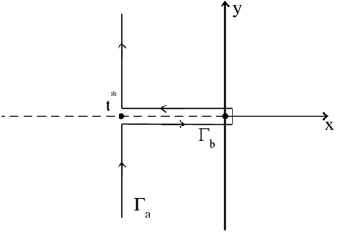
Figure 7: Steepest descent path in Eq. (138).

The point $t=0$ lies on the steepest ascent path issuing from the saddle point at $t^{*}$ and hence it will dominate the integral as $V\gg 1$ whenever $t^{*}=O(1)$ as $V\gg 1$. In this case only the paths $\Gamma_{b}$ contribute and a straightforward calculation leads to Eq. (125).

To study the behaviour in the critical region $\sqrt{V|\phi_{0}^{\prime\prime}|}t^{*}=O(1)$ as $V\gg 1$, it is convenient to notice that the steepest descent path $\Gamma_{a}+\Gamma_{b}$ can be deformed into the imaginary axis $x=0$ without changing the value of the integral. Taking $t=iy/\sqrt{V|\phi_{0}^{\prime\prime}|}$ the integral becomes:

$${\mathcal{N}}_{-}(\xi) =\frac{1}{[V|\phi_{0}^{\prime\prime}|]^{1/4}}\int_{-\infty}^{+\infty}\frac{dy}{2\pi}\,(iy)^{-1/2}e^{-y^{2}/2-i\xi y}$$

$$=\frac{1}{\sqrt{2\pi}}\frac{e^{-\xi^{2}/4}\,D_{-1/2}(\xi)}{[V|\phi_{0}^{\prime\prime}|]^{1/4}}\,,$$ (139)

where $\xi$ is defined in Eq. (130), which with Eq. (137) leads to Eq. (133). However, notice that now $\xi<0$ because we are in the condensed phase. Using the asymptotic expansion $D_{-1/2}(-|\xi|)\sim e^{\xi^{2}/4}\,/\sqrt{|\xi|}$ valid for $-\xi\gg 1$ Eq. (133) reduces to

$$P_{\rm match}(Q,V)=\frac{e^{-V\phi(-\lambda_{0}^{-};q)}}{\sqrt{2\pi V(q_{\delta}^{-}-q)}},$$ (140)

and matches asymptotically Eq. (125). Thus, from Eq. (135), the uniform asymptotic approximation to Eq. (122) as $V\gg 1$ for $q\leq q_{\delta}^{-}$ reads

$$P(Q;V)={\cal N}_{-}(\xi)\,e^{-V\phi(-\lambda_{0}^{-};q)}.$$ (141)

Notice that close to $q_{\delta}^{-}$, inside the critical region, $P(Q;V)$ is given by Eq. (133) regardless of $q$ being larger or smaller than $q_{\delta}^{-}$. The only difference is the sign of $\xi$. As a consequence $P(Q;V)$ is regular across the transition between the two phases. The singularity shows up only in the strict $V\to\infty$ limit.

Appendix B

In this Appendix we shortly discuss the case of $\alpha=0$, in which case the frequency $\omega(\mathbf{k})$ becomes $\mathbf{k}$-independent and the condensation transition disappears. If $\alpha=0$ the system reduces to that of $N$ harmonic oscillators of equal frequency $\omega$ and the Eq. (97) is replaced by:

$$P(Q,N)=\int_{\Gamma}\frac{dz}{2\pi i}\,e^{-N\phi(z;q)},$$ (142)

where

$$\phi(z;q)=qz+\frac{1}{2}\ln\left[\frac{(\lambda_{+}-z)(z+\lambda_{-})}{\lambda_{+}\lambda_{-}}\right],$$ (143)

and $q=Q/N$ is the exchanged heat per oscillator. In the large $N$ limit the integral is dominated by the saddle point $x^{*}$ on the real axis located at the stationary point of $\phi(z;q)$:

$$\phi^{\prime}(x^{*};q)=0\ \Rightarrow\ q=\frac{1}{2}\left[\frac{1}{\lambda_{+}-x^{*}}-\frac{1}{\lambda_{-}+x^{*}}\right].$$ (144)

Solving this equation one finds

$$x^{*}=\frac{1}{2}(\lambda_{+}-\lambda_{-})+\frac{1}{2q}\bigl{(}\sqrt{\Delta}-1\bigr{)},$$ (145)

with $\Delta=1+q^{2}(\lambda_{+}+\lambda_{-})^{2}$. It is not difficult to see that $-\lambda_{-}<x^{*}<\lambda_{+}$ for all value of $q$ and hence condensation cannot occur.

Near the saddle point the steepest descent path is parallel to the imaginary axis, and

$$P(Q,N)=\frac{1}{\sqrt{-2\pi N\phi^{\prime\prime}(x^{*};q)}}\,e^{-N\phi(x^{*};q)}.$$ (146)

as $N\gg 1$. Using Eq. (145) one finds

$$\phi(x^{*};q)=\frac{1}{2}\left[(\lambda_{+}-\lambda_{-})q+\sqrt{\Delta}-1+\ln\Bigl{[}\frac{a}{2q^{2}}(\sqrt{\Delta}-1)\Bigr{]}\right],$$ (147)

and

$$\phi^{\prime\prime}(x^{*};q)=-\frac{q^{2}(\lambda_{+}+\lambda_{-})^{2}+(\sqrt{\Delta}-1)^{2}}{(\sqrt{\Delta}-1)^{2}}\,q^{2}.$$ (148)

Hence

$$\frac{1}{N}{\mathcal{K}}(Q)=(\lambda_{-}-\lambda_{+})\,q$$ (149)

because $\Delta$ is even in $q$.

References

- (1) For a recent review of the subject see U. Seifert, Rep. Progr. Phys. 75, 126001 (2012).
- (2) G. M. Wang, E. M. Sevick, E. Mittag, D. J. Searles, and D. J. Evans, Phys. Rev. Lett. 89, 050601 (2002).
- (3) R. van Zon and E. G. D. Cohen, Phys. Rev. E 67 046102, (2003).
- (4) A. Imparato, L. Peliti, G. Pesce, G. Rusciano, A. Sasso, Phys. Rev. E 76, 050101(R) (2007).
- (5) K. Kim, C. Kwon, and H. Park, Phys. Rev. E 90, 032117 (2014).
- (6) A. Sarracino, D. Villamaina, G. Gradenigo and A. Puglisi, Europhys. Lett. 92 34001, (2010).
- (7) A. Naert, Europhys. Lett. 97, 20010 (2012).
- (8) A. Gnoli, A. Sarracino, A. Puglisi and A. Petri, Phys. Rev. E 87, 052209 (2013).
- (9) J. Farago, J. Stat. Phys. 107, 781 (2002); P. Visco, J. Stat. Mech. P06006 (2006); H. C. Fogedby and A. Imparato, J. Stat. Mech. P05015 (2011).
- (10) S. Joubaud, N. B. Garnier and S. Ciliberto, J. Stat. Mech. P09018 (2007).
- (11) A. Crisanti, A. Puglisi and D. Villamaina, Phys. Rev. E 85, 061127 (2012).
- (12) G. Gradenigo, A. Puglisi, A. Sarracino, U. Marini Bettolo Marconi, Phys. Rev. E 85, 031112 (2012).
- (13) G. Gradenigo, A. Puglisi, A. Sarracino, H. Touchette, J. Phys. A: Math. Theor. 46, 335002 (2013).
- (14) N. Kumar, S. Ramaswamy, and S. K. Sood, Phys. Rev. Lett. 106, 118001 (2011).
- (15) P. I. Hurtado, C. P. Espigares, J. J. del Pozo and P. L. Garrido, Proc. Natl. Acd. Sci. U.S.A. 108, 7704 (2011); P. I. Hurtado and P. L. Garrido, Phys. Rev. Lett. 107, 180601 (2011); C. P. Espigares, P. L. Garrido and P. I. Hurtado, Phys. Rev. E 87, 032115 (2013); P. I. Hurtado, C. P. Espigares, J. J. del Pozo and P. L. Garrido, J. Stat. Phys. 154, 214 (2014).
- (16) N. Goldenfeld, Lectures on Phase Transitions and The Renormalization Group, Addison-Wesley Publishing Co., Reading, Massachusetts (1992); P. Gaspard, J. Stat. Mech.: Th. Exp. P08021 (2012); D. Lacoste and P. Gaspard, J. Stat. Mech. P11018 (2015).
- (17) A Puglisi, L. Rondoni and A. Vulpiani, J. Stat. Mech. (2006) P08010.
- (18) M. Baiesi, T. Jacobs, C. Maes, and N. S. Skantzos, Phys. Rev. E 74, 021111 (2006).
- (19) A Rákos and R. J. Harris, J. Stat. Mech. (2008) P05005.
- (20) J. D. Noh and J.-M. Park, Phys. Rev. Lett. 108, 240603 (2012).
- (21) A. Crisanti and F. Ritort, Europhys. Lett. 66, 253 (2004).
- (22) A. Crisanti, M. Picco, and F. Ritort, Phys. Rev. Lett. 110, 080601 (2013).
- (23) F. Zamponi, F. Bonetto, L. F. Cugliandolo, J. Kurchan, J. Stat. Mech. (2005) P09013.
- (24) H. Touchette, Phys. Rep. 478, 1 (2009).
- (25) Large Deviations in Physics, edited by A. Vulpiani, F. Cecconi, M. Cencini, A. Puglisi, and D. Vergni (Springer, Berlin, 2014)
- (26) F. Corberi, G. Gonnella, A. Piscitelli and M. Zannetti, J. Phys. A: Math. Theor. 46, 042001 (2013).
- (27) M. Zannetti, F. Corberi and G. Gonnella, Phys. Rev. E 90, 012143 (2014).
- (28) M. Zannetti, F. Corberi, G. Gonnella and A. Piscitelli, Commun. Theor. Phys. 62, 555 (2014).
- (29) G. Gallavotti and E. D. G. Cohen, Phys. Rev. Lett. 50, 2694 (1995).
- (30) C. Maes, J. Stat. Phys. 95, 367 (1999).
- (31) K. Gawedzki, arXiv:1308.1518.
- (32) J. R. Gomez-Solano, A. Petrosyan, and S. Ciliberto, Phys. Rev. Lett. 106, 200602 (2011).
- (33) D. Chatterjee and B. J. Cherayil, Phys. Rev. E 82, 051104 (2010).
- (34) D. S. P. Salazar and S. A. Lira, J. Phys. A: Math. Theor. 49, 465001 (2016).
- (35) For details on systems of this type, see Refs. Gonnella ; Jo ; Pechino .
- (36) S. K. Ma, Modern Theory of Critical Phenomena, Benjamin, Reading, Massachusetts (1976).
- (37) To perform the asymptotic analysis of Eq. (97) we assume that the variable and all parameters entering into the integral have been made dimensionless. The correct dimension of can be reestablished by multiplying the result by, e.g, , or any other parameter with dimension . This factor, nevertheless, can be always absorbed into the normalization term and is not considered in the computation.
- (38) K. Huang, Statistical Mechanics, John Wiley and Sons, New York 1967; R. K. Pathria and P. D. Beale, Statistical Mechanics, 3d Edition, Elsevier, Amsterdam 2011.
- (39) N. Merhav and Y. Kafri, J. Stat. Mech. P02011 (2010).
- (40) M. Filiasi, G.Livan, M. Marsili, M. Peressi, E. Vesselli and E. Zarinelli, J. Stat. Mech. (2014) P09030; M. Filiasi, E. Zarinelli, E. Vesselli and M. Marsili, arXiv:1309.7795v1; L. Ferretti, M. Mamino and G. Bianconi, Phys. Rev. E 89, 042810 (2014).
- (41) R.J. Harris, A. Rákos, and G.M. Schuetz, J. Stat. Mech. P08003 (2005); A. Gambassi and A. Silva, Phys. Rev. Lett. 109, 250602 (2012); J. Szavits-Nossan, M. R. Evans and S. N. Majumdar, Phys. Rev. Lett. 112, 020602 (2014); M. Zannetti, Eur. Phys. Lett. 111, 20004 (2015); F. Corberi, J. Phys. A: Math. Theor. 48, 465003 (2015).
- (42) T. H. Berlin and M. Kac, Phys. Rev. 86, 821 (1952).
- (43) When is not too close to the difference between and as is and can be included into the corrections. In this case Eq. (118) gives a valid uniform asymptotic approximation to , and its derivatives.
- (44) I. S. Gradshteyn, and I. M. Ryzhik, Tables of Integrals, Series, and Products, 6th ed. San Diego, CA: Academic Press, 2000.