Learning Certifiably Optimal Rule Lists for Categorical Data

Abstract

We present the design and implementation of a custom discrete optimization technique for building rule lists over a categorical feature space. Our algorithm produces rule lists with optimal training performance, according to the regularized empirical risk, with a certificate of optimality. By leveraging algorithmic bounds, efficient data structures, and computational reuse, we achieve several orders of magnitude speedup in time and a massive reduction of memory consumption. We demonstrate that our approach produces optimal rule lists on practical problems in seconds. Our results indicate that it is possible to construct optimal sparse rule lists that are approximately as accurate as the COMPAS proprietary risk prediction tool on data from Broward County, Florida, but that are completely interpretable. This framework is a novel alternative to CART and other decision tree methods for interpretable modeling.

Keywords: rule lists, decision trees, optimization, interpretable models, criminal justice applications

1 Introduction

As machine learning continues to gain prominence in socially-important decision-making, the interpretability of predictive models remains a crucial problem. Our goal is to build models that are highly predictive, transparent, and easily understood by humans. We use rule lists, also known as decision lists, to achieve this goal. Rule lists are predictive models composed of if-then statements; these models are interpretable because the rules provide a reason for each prediction (Figure 1).

Constructing rule lists, or more generally, decision trees, has been a challenge for more than 30 years; most approaches use greedy splitting techniques (Rivest, 1987; Breiman et al., 1984; Quinlan, 1993). Recent approaches use Bayesian analysis, either to find a locally optimal solution (Chipman et al., 1998) or to explore the search space (Letham et al., 2015; Yang et al., 2017). These approaches achieve high accuracy while also managing to run reasonably quickly. However, despite the apparent accuracy of the rule lists generated by these algorithms, there is no way to determine either if the generated rule list is optimal or how close it is to optimal, where optimality is defined with respect to minimization of a regularized loss function.

if $(age=18-20){\bf~{}and~{}}(sex=male)$ then predict $yes$

else if $(age=21-23){\bf~{}and~{}}(priors=2-3)$ then predict $yes$

else if $(priors>3)$ then predict $yes$

else predict $no$

Figure 1: An example rule list that predicts two-year recidivism for the ProPublica data set, found by CORELS.

Optimality is important, because there are societal implications for a lack of optimality. Consider the ProPublica article on the Correctional Offender Management Profiling for Alternative Sanctions (COMPAS) recidivism prediction tool (Larson et al., 2016). It highlights a case where a black box, proprietary predictive model is being used for recidivism prediction. The authors hypothesize that the COMPAS scores are racially biased, but since the model is not transparent, no one (outside of the creators of COMPAS) can determine the reason or extent of the bias (Larson et al., 2016), nor can anyone determine the reason for any particular prediction. By using COMPAS, users implicitly assumed that a transparent model would not be sufficiently accurate for recidivism prediction, i.e., they assumed that a black box model would provide better accuracy. We wondered whether there was indeed no transparent and sufficiently accurate model. Answering this question requires solving a computationally hard problem. Namely, we would like to both find a transparent model that is optimal within a particular pre-determined class of models and produce a certificate of its optimality, with respect to the regularized empirical risk. This would enable one to say, for this problem and model class, with certainty and before resorting to black box methods, whether there exists a transparent model. While there may be differences between training and test performance, finding the simplest model with optimal training performance is prescribed by statistical learning theory.

To that end, we consider the class of rule lists assembled from pre-mined frequent itemsets and search for an optimal rule list that minimizes a regularized risk function, $R$. This is a hard discrete optimization problem. Brute force solutions that minimize $R$ are computationally prohibitive due to the exponential number of possible rule lists. However, this is a worst case bound that is not realized in practical settings. For realistic cases, it is possible to solve fairly large cases of this problem to optimality, with the careful use of algorithms, data structures, and implementation techniques.

We develop specialized tools from the fields of discrete optimization and artificial intelligence. Specifically, we introduce a special branch-and bound algorithm, called Certifiably Optimal RulE ListS (CORELS), that provides the optimal solution according to the training objective, along with a certificate of optimality. The certificate of optimality means that we can investigate how close other models (e.g., models provided by greedy algorithms) are to optimal.

Within its branch-and-bound procedure, CORELS maintains a lower bound on the minimum value of $R$ that each incomplete rule list can achieve. This allows CORELS to prune an incomplete rule list (and every possible extension) if the bound is larger than the error of the best rule list that it has already evaluated. The use of careful bounding techniques leads to massive pruning of the search space of potential rule lists. The algorithm continues to consider incomplete and complete rule lists until it has either examined or eliminated every rule list from consideration. Thus, CORELS terminates with the optimal rule list and a certificate of optimality.

The efficiency of CORELS depends on how much of the search space our bounds allow us to prune; we seek a tight lower bound on $R$. The bound we maintain throughout execution is a maximum of several bounds that come in three categories. The first category of bounds are those intrinsic to the rules themselves. This category includes bounds stating that each rule must capture sufficient data; if not, the rule list is provably non-optimal. The second type of bound compares a lower bound on the value of $R$ to that of the current best solution. This allows us to exclude parts of the search space that could never be better than our current solution. Finally, our last type of bound is based on comparing incomplete rule lists that capture the same data and allows us to pursue only the most accurate option. This last class of bounds is especially important—without our use of a novel symmetry-aware map, we are unable to solve most problems of reasonable scale. This symmetry-aware map keeps track of the best accuracy over all observed permutations of a given incomplete rule list.

We keep track of these bounds using a modified prefix tree, a data structure also known as a trie. Each node in the prefix tree represents an individual rule; thus, each path in the tree represents a rule list such that the final node in the path contains metrics about that rule list. This tree structure, together with a search policy and sometimes a queue, enables a variety of strategies, including breadth-first, best-first, and stochastic search. In particular, we can design different best-first strategies by customizing how we order elements in a priority queue. In addition, we are able to limit the number of nodes in the trie and thereby enable tuning of space-time tradeoffs in a robust manner. This trie structure is a useful way of organizing the generation and evaluation of rule lists.

We evaluated CORELS on a number of publicly available data sets. Our metric of success was 10-fold cross-validated prediction accuracy on a subset of the data. These data sets involve hundreds of rules and thousands of observations. CORELS is generally able to find an optimal rule list in a matter of seconds and certify its optimality within about 10 minutes. We show that we are able to achieve better or similar out-of-sample accuracy on these data sets compared to the popular greedy algorithms, CART and C4.5.

CORELS targets large (not massive) problems, where interpretability and certifiable optimality are important. We illustrate the efficacy of our approach using (1) the ProPublica COMPAS data set (Larson et al., 2016), for the problem of two-year recidivism prediction, and (2) stop-and-frisk data sets from the NYPD (New York Police Department, 2016) and the NYCLU (New York Civil Liberties Union, 2014), to predict whether a weapon will be found on a stopped individual who is frisked or searched. On these data, we produce certifiably optimal, interpretable rule lists that achieve the same accuracy as approaches such as random forests. This calls into question the need for use of a proprietary, black box algorithm for recidivism prediction.

Our work overlaps with the thesis of Larus-Stone (2017). We have also written a preliminary conference version of this article (Angelino et al., 2017), and a report highlighting systems optimizations of our implementation (Larus-Stone et al., 2018); the latter includes additional empirical measurements not presented here.

Our code is at https://github.com/nlarusstone/corels, where we provide the C++ implementation we used in our experiments (§6). Kaxiras and Saligrama (2018) have also created an interactive web interface at https://corels.eecs.harvard.edu, where a user can upload data and run CORELS from a browser.

2 Related Work

Since every rule list is a decision tree and every decision tree can be expressed as an equivalent rule list, the problem we are solving is a version of the “optimal decision tree” problem, though regularization changes the nature of the problem (as shown through our bounds). The optimal decision tree problem is computationally hard, though since the late 1990’s, there has been research on building optimal decision trees using optimization techniques (Bennett and Blue, 1996; Dobkin et al., 1996; Farhangfar et al., 2008). A particularly interesting paper along these lines is that of Nijssen and Fromont (2010), who created a “bottom-up” way to form optimal decision trees. Their method performs an expensive search step, mining all possible leaves (rather than all possible rules), and uses those leaves to form trees. Their method can lead to memory problems, but it is possible that these memory issues can be mitigated using the theorems in this paper. None of these methods used the tight bounds and data structures of CORELS.

Because the optimal decision tree problem is hard, there are a huge number of algorithms such as CART (Breiman et al., 1984) and C4.5 (Quinlan, 1993) that do not perform exploration of the search space beyond greedy splitting. Similarly, there are decision list and associative classification methods that construct rule lists iteratively in a greedy way (Rivest, 1987; Liu et al., 1998; Li et al., 2001; Yin and Han, 2003; Sokolova et al., 2003; Marchand and Sokolova, 2005; Vanhoof and Depaire, 2010; Rudin et al., 2013). Some exploration of the search space is done by Bayesian decision tree methods (Dension et al., 1998; Chipman et al., 2002, 2010) and Bayesian rule-based methods (Letham et al., 2015; Yang et al., 2017). The space of trees of a given depth is much larger than the space of rule lists of that same depth, and the trees within the Bayesian tree algorithms are grown in a top-down greedy way. Because of this, authors of Bayesian tree algorithms have noted that their MCMC chains tend to reach only locally optimal solutions. The RIPPER algorithm (Cohen, 1995) is similar to the Bayesian tree methods in that it grows, prunes, and then locally optimizes. The space of rule lists is smaller than that of trees, and has simpler structure. Consequently, Bayesian rule list algorithms tend to be more successful at escaping local minima and can introduce methods of exploring the search space that exploit this structure—these properties motivate our focus on lists. That said, the tightest bounds for the Bayesian lists (namely, those of Yang et al., 2017, upon whose work we build), are not nearly as tight as those of CORELS.

Tight bounds, on the other hand, have been developed for the (immense) literature on building disjunctive normal form (DNF) models; a good example of this is the work of Rijnbeek and Kors (2010). For models of a given size, since the class of DNF’s is a proper subset of decision lists, our framework can be restricted to learn optimal DNF’s. The field of DNF learning includes work from the fields of rule learning/induction (e.g., early algorithms by Michalski, 1969; Clark and Niblett, 1989; Frank and Witten, 1998) and associative classification (Vanhoof and Depaire, 2010). Most papers in these fields aim to carefully guide the search through the space of models. If we were to place a restriction on our code to learn DNF’s, which would require restricting predictions within the list to the positive class only, we could potentially use methods from rule learning and associative classification to help order CORELS’ queue, which would in turn help us eliminate parts of the search space more quickly.

Some of our bounds, including the minimum support bound (§3.7, Theorem 10), come from Rudin and Ertekin (2016), who provide flexible mixed-integer programming (MIP) formulations using the same objective as we use here; MIP solvers in general cannot compete with the speed of CORELS.

CORELS depends on pre-mined rules, which we obtain here via enumeration. The literature on association rule mining is huge, and any method for rule mining could be reasonably substituted.

CORELS’ main use is for producing interpretable predictive models. There is a growing interest in interpretable (transparent, comprehensible) models because of their societal importance (see Rüping, 2006; Bratko, 1997; Dawes, 1979; Vellido et al., 2012; Giraud-Carrier, 1998; Holte, 1993; Shmueli, 2010; Huysmans et al., 2011; Freitas, 2014). There are now regulations on algorithmic decision-making in the European Union on the “right to an explanation” (Goodman and Flaxman, 2016) that would legally require interpretability of predictions. There is work in both the DNF literature (Rückert and Raedt, 2008) and decision tree literature (Garofalakis et al., 2000) on building interpretable models. Interpretable models must be so sparse that they need to be heavily optimized; heuristics tend to produce either inaccurate or non-sparse models.

Interpretability has many meanings, and it is possible to extend the ideas in this work to other definitions of interpretability; these rule lists may have exotic constraints that help with ease-of-use. For example, Falling Rule Lists (Wang and Rudin, 2015a) are constrained to have decreasing probabilities down the list, which makes it easier to assess whether an observation is in a high risk subgroup. In parallel to this paper, we have been working on an algorithm for Falling Rule Lists (Chen and Rudin, 2018) with bounds similar to those presented here, but even CORELS’ basic support bounds do not hold for the falling case, which is much more complicated. One advantage of the approach taken by Chen and Rudin (2018) is that it can handle class imbalance by weighting the positive and negative classes differently; this extension is possible in CORELS but not addressed here.

The models produced by CORELS are predictive only; they cannot be used for policy-making because they are not causal models, they do not include the costs of true and false positives, nor the cost of gathering information. It is possible to adapt CORELS’ framework for causal inference (Wang and Rudin, 2015b), dynamic treatment regimes (Zhang et al., 2015), or cost-sensitive dynamic treatment regimes (Lakkaraju and Rudin, 2017) to help with policy design. CORELS could potentially be adapted to handle these kinds of interesting problems.

3 Learning Optimal Rule Lists

In this section, we present our framework for learning certifiably optimal rule lists. First, we define our setting and useful notation (§3.1) and then the objective function we seek to minimize (§3.2). Next, we describe the principal structure of our optimization algorithm (§3.3), which depends on a hierarchically structured objective lower bound (§3.4). We then derive a series of additional bounds that we incorporate into our algorithm, because they enable aggressive pruning of our state space.

3.1 Notation

We restrict our setting to binary classification, where rule lists are Boolean functions; this framework is straightforward to generalize to multi-class classification. Let ${\{(x_{n},y_{n})\}_{n=1}^{N}}$ denote training data, where ${x_{n}\in\{0,1\}^{J}}$ are binary features and ${y_{n}\in\{0,1\}}$ are labels. Let ${\mathbf{x}=\{x_{n}\}_{n=1}^{N}}$ and ${\mathbf{y}=\{y_{n}\}_{n=1}^{N}}$, and let ${x_{n,j}}$ denote the $j$-th feature of $x_{n}$.

A rule list ${{d}=(r_{1},r_{2},\dots,r_{K},r_{0})}$ of length ${K\geq 0}$ is a ${(K+1)}$-tuple consisting of $K$ distinct association rules, ${r_{k}=p_{k}\rightarrow q_{k}}$, for ${k=1,\dots,K}$, followed by a default rule $r_{0}$. Figure 2 illustrates a rule list, ${{d}=}$ ${(r_{1},r_{2},r_{3},r_{0})}$, which for clarity, we sometimes call a $K$-rule list. An association rule ${r=p\rightarrow q}$ is an implication corresponding to the conditional statement, “if $p$, then $q$.” In our setting, an antecedent $p$ is a Boolean assertion that evaluates to either true or false for each datum $x_{n}$, and a consequent $q$ is a label prediction. For example, ${(x_{n,1}=0)\wedge(x_{n,3}=1)\rightarrow}$ ${(y_{n}=1)}$ is an association rule. The final default rule $r_{0}$ in a rule list can be thought of as a special association rule ${p_{0}\rightarrow q_{0}}$ whose antecedent $p_{0}$ simply asserts true.

if $(age=18-20){\bf~{}and~{}}(sex=male)$ then predict $yes$

else if $(age=21-23){\bf~{}and~{}}(priors=2-3)$ then predict $yes$

else if $(priors>3)$ then predict $yes$

else predict $no$

if $p_{1}$ then predict $q_{1}$

else if $p_{2}$ then predict $q_{2}$

else if $p_{3}$ then predict $q_{3}$

else predict $q_{0}$

Figure 2: The rule list ${{d}=(r_{1},r_{2},r_{3},r_{0})}$. Each rule is of the form ${r_{k}=p_{k}\rightarrow q_{k}}$, for all ${k=0,\dots,3}$. We can also express this rule list as ${{d}=(d_{p},\delta_{p},q_{0},K)}$, where ${d_{p}=(p_{1},p_{2},p_{3})}$, ${\delta_{p}=(1,1,1,1)}$, ${q_{0}=0}$, and ${K=3}$. This is the same 3-rule list as in Figure 1, that predicts two-year recidivism for the ProPublica data set.

Let ${{d}=(r_{1},r_{2},\dots,r_{K},r_{0})}$ be a $K$-rule list, where ${r_{k}=p_{k}\rightarrow q_{k}}$ for each ${k=0,\dots,K}$. We introduce a useful alternate rule list representation: ${{d}=(d_{p},\delta_{p},q_{0},K)}$, where we define ${d_{p}=(p_{1},\dots,p_{K})}$ to be ${d}$’s prefix, ${\delta_{p}=(q_{1},\dots,q_{K})\in\{0,1\}^{K}}$ gives the label predictions associated with $d_{p}$, and ${q_{0}\in\{0,1\}}$ is the default label prediction. For example, for the rule list in Figure 1, we would write ${{d}=(d_{p},\delta_{p},q_{0},K)}$, where ${d_{p}=(p_{1},p_{2},p_{3})}$, ${\delta_{p}=(1,1,1)}$, ${q_{0}=0}$, and ${K=3}$. Note that ${((),(),q_{0},0)}$ is a well-defined rule list with an empty prefix; it is completely defined by a single default rule.

Let ${d_{p}=(p_{1},\dots,p_{k},\dots,p_{K})}$ be an antecedent list, then for any ${k\leq K}$, we define ${d_{p}^{k}=}$ ${(p_{1},\dots,p_{k})}$ to be the $k$-prefix of $d_{p}$. For any such $k$-prefix $d_{p}^{k}$, we say that $d_{p}$ starts with $d_{p}^{k}$. For any given space of rule lists, we define $\sigma(d_{p})$ to be the set of all rule lists whose prefixes start with $d_{p}$:

$$\sigma(d_{p})=\{(d_{p}^{\prime},\delta_{p}^{\prime},q_{0}^{\prime},K^{\prime}):d_{p}^{\prime}\textnormal{ starts with }d_{p}\}.$$ (1)

If ${d_{p}=(p_{1},\dots,p_{K})}$ and ${d_{p}^{\prime}=(p_{1},\dots,p_{K},p_{K+1})}$ are two prefixes such that $d_{p}^{\prime}$ starts with $d_{p}$ and extends it by a single antecedent, we say that $d_{p}$ is the parent of $d_{p}^{\prime}$ and that $d_{p}^{\prime}$ is a child of $d_{p}$.

A rule list ${d}$ classifies datum $x_{n}$ by providing the label prediction $q_{k}$ of the first rule $r_{k}$ whose antecedent $p_{k}$ is true for $x_{n}$. We say that an antecedent $p_{k}$ of antecedent list $d_{p}$ captures $x_{n}$ in the context of $d_{p}$ if $p_{k}$ is the first antecedent in $d_{p}$ that evaluates to true for $x_{n}$. We also say that a prefix captures those data captured by its antecedents; for a rule list ${{d}=(d_{p},\delta_{p},q_{0},K)}$, data not captured by the prefix $d_{p}$ are classified according to the default label prediction $q_{0}$.

Let $\beta$ be a set of antecedents. We define ${\textnormal{cap}(x_{n},\beta)=1}$ if an antecedent in $\beta$ captures datum $x_{n}$, and 0 otherwise. For example, let $d_{p}$ and $d_{p}^{\prime}$ be prefixes such that $d_{p}^{\prime}$ starts with $d_{p}$, then $d_{p}^{\prime}$ captures all the data that $d_{p}$ captures:

$$\{x_{n}:\textnormal{cap}(x_{n},d_{p})\}\subseteq\{x_{n}:\textnormal{cap}(x_{n},d_{p}^{\prime})\}.$$

Now let $d_{p}$ be an ordered list of antecedents, and let $\beta$ be a subset of antecedents in $d_{p}$. Let us define ${\textnormal{cap}(x_{n},\beta\,|\,d_{p})=1}$ if $\beta$ captures datum $x_{n}$ in the context of $d_{p}$, i.e., if the first antecedent in $d_{p}$ that evaluates to true for $x_{n}$ is an antecedent in $\beta$, and 0 otherwise. Thus, ${\textnormal{cap}(x_{n},\beta\,|\,d_{p})=1}$ only if ${\textnormal{cap}(x_{n},\beta)=1}$; ${\textnormal{cap}(x_{n},\beta\,|\,d_{p})=0}$ either if ${\textnormal{cap}(x_{n},\beta)=0}$, or if ${\textnormal{cap}(x_{n},\beta)=1}$ but there is an antecedent $\alpha$ in $d_{p}$, preceding all antecedents in $\beta$, such that ${\textnormal{cap}(x_{n},\alpha)=1}$. For example, if ${d_{p}=(p_{1},\dots,p_{k},\dots,p_{K})}$ is a prefix, then

$$\textnormal{cap}(x_{n},p_{k}\,|\,d_{p})=\left(\bigwedge_{k^{\prime}=1}^{k-1}\neg\,\textnormal{cap}(x_{n},p_{k^{\prime}})\right)\wedge\textnormal{cap}(x_{n},p_{k})$$

indicates whether antecedent $p_{k}$ captures datum $x_{n}$ in the context of $d_{p}$. Now, define ${\textnormal{supp}(\beta,\mathbf{x})}$ to be the normalized support of $\beta$,

$$\textnormal{supp}(\beta,\mathbf{x})=\frac{1}{N}\sum_{n=1}^{N}\textnormal{cap}(x_{n},\beta),$$ (2)

and similarly define ${\textnormal{supp}(\beta,\mathbf{x}\,|\,d_{p})}$ to be the normalized support of $\beta$ in the context of $d_{p}$,

$$\textnormal{supp}(\beta,\mathbf{x}\,|\,d_{p})=\frac{1}{N}\sum_{n=1}^{N}\textnormal{cap}(x_{n},\beta\,|\,d_{p}),$$ (3)

Next, we address how empirical data constrains rule lists. Given training data ${(\mathbf{x},\mathbf{y})}$, an antecedent list ${d_{p}=(p_{1},\dots,p_{K})}$ implies a rule list ${{d}=(d_{p},\delta_{p},q_{0},K)}$ with prefix $d_{p}$, where the label predictions ${\delta_{p}=(q_{1},\dots,q_{K})}$ and $q_{0}$ are empirically set to minimize the number of misclassification errors made by the rule list on the training data. Thus for ${1\leq k\leq K}$, label prediction $q_{k}$ corresponds to the majority label of data captured by antecedent $p_{k}$ in the context of $d_{p}$, and the default $q_{0}$ corresponds to the majority label of data not captured by $d_{p}$. In the remainder of our presentation, whenever we refer to a rule list with a particular prefix, we implicitly assume these empirically determined label predictions.

Our method is technically an associative classification method since it leverages pre-mined rules.

3.2 Objective Function

We define a simple objective function for a rule list ${{d}=(d_{p},\delta_{p},q_{0},K)}$:

$$R({d},\mathbf{x},\mathbf{y})=\ell({d},\mathbf{x},\mathbf{y})+{\lambda}K.$$ (4)

This objective function is a regularized empirical risk; it consists of a loss $\ell({d},\mathbf{x},\mathbf{y})$, measuring misclassification error, and a regularization term that penalizes longer rule lists. $\ell({d},\mathbf{x},\mathbf{y})$ is the fraction of training data whose labels are incorrectly predicted by ${d}$. In our setting, the regularization parameter ${{\lambda}\geq 0}$ is a small constant; e.g., ${{\lambda}=0.01}$ can be thought of as adding a penalty equivalent to misclassifying $1\%$ of data when increasing a rule list’s length by one association rule.

3.3 Optimization Framework

Our objective has structure amenable to global optimization via a branch-and-bound framework. In particular, we make a series of important observations, each of which translates into a useful bound, and that together interact to eliminate large parts of the search space. We discuss these in depth in what follows:

• Lower bounds on a prefix also hold for every extension of that prefix. (§3.4, Theorem 1)

• If a rule list is not accurate enough with respect to its length, we can prune all extensions of it. (§3.4, Lemma 2)

• We can calculate a priori an upper bound on the maximum length of an optimal rule list. (§3.5, Theorem 6)

• Each rule in an optimal rule list must have support that is sufficiently large. This allows us to construct rule lists from frequent itemsets, while preserving the guarantee that we can find a globally optimal rule list from pre-mined rules. (§3.7, Theorem 10)

• Each rule in an optimal rule list must predict accurately. In particular, the number of observations predicted correctly by each rule in an optimal rule list must be above a threshold. (§3.7, Theorem 11)

• We need only consider the optimal permutation of antecedents in a prefix; we can omit all other permutations. (§3.10, Theorem 15 and Corollary 16)

• If multiple observations have identical features and opposite labels, we know that any model will make mistakes. In particular, the number of mistakes on these observations will be at least the number of observations with the minority label. (§3.14, Theorem 20)

3.4 Hierarchical Objective Lower Bound

We can decompose the misclassification error in (4) into two contributions corresponding to the prefix and the default rule:

$$\ell({d},\mathbf{x},\mathbf{y})\equiv\ell_{p}(d_{p},\delta_{p},\mathbf{x},\mathbf{y})+\ell_{0}(d_{p},q_{0},\mathbf{x},\mathbf{y}),$$

where ${d_{p}=(p_{1},\dots,p_{K})}$ and ${\delta_{p}=(q_{1},\dots,q_{K})}$;

$$\ell_{p}(d_{p},\delta_{p},\mathbf{x},\mathbf{y})=\frac{1}{N}\sum_{n=1}^{N}\sum_{k=1}^{K}\textnormal{cap}(x_{n},p_{k}\,|\,d_{p})\wedge\mathds{1}[q_{k}\neq y_{n}]$$

is the fraction of data captured and misclassified by the prefix, and

$$\ell_{0}(d_{p},q_{0},\mathbf{x},\mathbf{y})=\frac{1}{N}\sum_{n=1}^{N}\neg\,\textnormal{cap}(x_{n},d_{p})\wedge\mathds{1}[q_{0}\neq y_{n}]$$

is the fraction of data not captured by the prefix and misclassified by the default rule. Eliminating the latter error term gives a lower bound $b(d_{p},\mathbf{x},\mathbf{y})$ on the objective,

$$b(d_{p},\mathbf{x},\mathbf{y})\equiv\ell_{p}(d_{p},\delta_{p},\mathbf{x},\mathbf{y})+{\lambda}K\leq R({d},\mathbf{x},\mathbf{y}),$$ (5)

where we have suppressed the lower bound’s dependence on label predictions $\delta_{p}$ because they are fully determined, given ${(d_{p},\mathbf{x},\mathbf{y})}$. Furthermore, as we state next in Theorem 1, $b(d_{p},\mathbf{x},\mathbf{y})$ gives a lower bound on the objective of any rule list whose prefix starts with $d_{p}$.

Theorem 1 (Hierarchical objective lower bound)

Define ${b(d_{p},\mathbf{x},\mathbf{y})}$ as in (5). Also, define $\sigma(d_{p})$ to be the set of all rule lists whose prefixes starts with $d_{p}$, as in (1). Let ${{d}=}$ ${(d_{p},\delta_{p},q_{0},K)}$ be a rule list with prefix $d_{p}$, and let ${{d}^{\prime}=(d_{p}^{\prime},\delta_{p}^{\prime},q_{0}^{\prime},K^{\prime})}$ $\in\sigma(d_{p})$ be any rule list such that its prefix $d_{p}^{\prime}$ starts with $d_{p}$ and ${K^{\prime}\geq K}$, then ${b(d_{p},\mathbf{x},\mathbf{y})\leq}$ ${R({d}^{\prime},\mathbf{x},\mathbf{y})}$.

Proof  Let ${d_{p}=(p_{1},\dots,p_{K})}$ and ${\delta_{p}=(q_{1},\dots,q_{K})}$; let ${d_{p}^{\prime}=(p_{1},\dots,p_{K},p_{K+1},\dots,p_{K^{\prime}})}$ and ${\delta_{p}^{\prime}=(q_{1},\dots,q_{K},q_{K+1},\dots,q_{K^{\prime}})}$. Notice that $d_{p}^{\prime}$ yields the same mistakes as $d_{p}$, and possibly additional mistakes:

$$\ell_{p}(d_{p}^{\prime},\delta_{p}^{\prime},\mathbf{x},\mathbf{y})=\frac{1}{N}\sum_{n=1}^{N}\sum_{k=1}^{K^{\prime}}\textnormal{cap}(x_{n},p_{k}\,|\,d_{p}^{\prime})\wedge\mathds{1}[q_{k}\neq y_{n}]$$

$$=\frac{1}{N}\sum_{n=1}^{N}\left(\sum_{k=1}^{K}\textnormal{cap}(x_{n},p_{k}\,|\,d_{p})\wedge\mathds{1}[q_{k}\neq y_{n}]+\sum_{k=K+1}^{K^{\prime}}\textnormal{cap}(x_{n},p_{k}\,|\,d_{p}^{\prime})\wedge\mathds{1}[q_{k}\neq y_{n}]\right)$$

$$=\ell_{p}(d_{p},\delta_{p},\mathbf{x},\mathbf{y})+\frac{1}{N}\sum_{n=1}^{N}\sum_{k=K+1}^{K^{\prime}}\textnormal{cap}(x_{n},p_{k}\,|\,d_{p}^{\prime})\wedge\mathds{1}[q_{k}\neq y_{n}]\geq\ell_{p}(d_{p},\delta_{p},\mathbf{x},\mathbf{y}),$$ (6)

where in the second equality we have used the fact that ${\textnormal{cap}(x_{n},p_{k}\,|\,d_{p}^{\prime})=\textnormal{cap}(x_{n},p_{k}\,|\,d_{p})}$ for ${1\leq k\leq K}$. It follows that

$$b(d_{p},\mathbf{x},\mathbf{y}) =\ell_{p}(d_{p},\delta_{p},\mathbf{x},\mathbf{y})+{\lambda}K$$

$$\leq\ell_{p}(d_{p}^{\prime},\delta_{p}^{\prime},\mathbf{x},\mathbf{y})+{\lambda}K^{\prime}=b(d_{p}^{\prime},\mathbf{x},\mathbf{y})\leq R({d}^{\prime},\mathbf{x},\mathbf{y}).$$ (7)

 

To generalize, consider a sequence of prefixes such that each prefix starts with all previous prefixes in the sequence. It follows that the corresponding sequence of objective lower bounds increases monotonically. This is precisely the structure required and exploited by branch-and-bound, illustrated in Algorithm 1.

Algorithm 1 Branch-and-bound for learning rule lists.

Input: Objective function $R({d},\mathbf{x},\mathbf{y})$, objective lower bound ${b(d_{p},\mathbf{x},\mathbf{y})}$, set of antecedents ${S=\{s_{m}\}_{m=1}^{M}}$, training data $(\mathbf{x},\mathbf{y})={\{(x_{n},y_{n})\}_{n=1}^{N}}$, initial best known rule list $d^{0}$ with objective ${R^{0}=R(d^{0},\mathbf{x},\mathbf{y})}$; $d^{0}$ could be obtained as output from another (approximate) algorithm, otherwise, $(d^{0},R^{0})=(\text{null},1)$ provide reasonable default values

Output: Provably optimal rule list $d^{*}$ with minimum objective $R^{*}$

$(d^{c},{R^{c}})\leftarrow(d^{0},R^{0})$ $\triangleright$ Initialize best rule list and objective

$Q\leftarrow$ queue$(\,[\,(\,)\,]\,)$ $\triangleright$ Initialize queue with empty prefix

while $Q$ not empty do $\triangleright$ Stop when queue is empty

     $d_{p}\leftarrow Q$.pop( ) $\triangleright$ Remove prefix $d_{p}$ from the queue

     ${d}\leftarrow(d_{p},\delta_{p},q_{0},K)$ $\triangleright$ Set label predictions $\delta_{p}$ and $q_{0}$ to minimize training error

     if $b(d_{p},\mathbf{x},\mathbf{y})<{R^{c}}$ then $\triangleright$ Bound: Apply Theorem 1

         $R\leftarrow R({d},\mathbf{x},\mathbf{y})$ $\triangleright$ Compute objective of $d_{p}$’s rule list ${d}$

         if $R<{R^{c}}$ then $\triangleright$ Update best rule list and objective

              $(d^{c},{R^{c}})\leftarrow({d},R)$

         end if

         for $s$ in $S$ do $\triangleright$ Branch: Enqueue $d_{p}$’s children

              if $s$ not in $d_{p}$ then

                  $Q$.push$(\,(d_{p},s)\,)$

              end if

         end for

     end if

end while

$(d^{*},R^{*})\leftarrow(d^{c},{R^{c}})$ $\triangleright$ Identify provably optimal solution

Specifically, the objective lower bound in Theorem 1 enables us to prune the state space hierarchically. While executing branch-and-bound, we keep track of the current best (smallest) objective ${R^{c}}$, thus it is a dynamic, monotonically decreasing quantity. If we encounter a prefix $d_{p}$ with lower bound ${b(d_{p},\mathbf{x},\mathbf{y})\geq{R^{c}}}$, then by Theorem 1, we do not need to consider any rule list ${{d}^{\prime}\in\sigma(d_{p})}$ whose prefix $d_{p}^{\prime}$ starts with $d_{p}$. For the objective of such a rule list, the current best objective provides a lower bound, i.e., ${R({d}^{\prime},\mathbf{x},\mathbf{y})\geq b(d_{p}^{\prime},\mathbf{x},\mathbf{y})\geq}$ ${b(d_{p},\mathbf{x},\mathbf{y})\geq{R^{c}}}$, and thus ${d}^{\prime}$ cannot be optimal.

Next, we state an immediate consequence of Theorem 1.

Lemma 2 (Objective lower bound with one-step lookahead)

Let $d_{p}$ be a $K$-prefix and let ${R^{c}}$ be the current best objective. If ${b(d_{p},\mathbf{x},\mathbf{y})+{\lambda}\geq{R^{c}}}$, then for any $K^{\prime}$-rule list ${{d}^{\prime}\in\sigma(d_{p})}$ whose prefix $d_{p}^{\prime}$ starts with $d_{p}$ and ${K^{\prime}>K}$, it follows that ${R({d}^{\prime},\mathbf{x},\mathbf{y})\geq{R^{c}}}$.

Proof  By the definition of the lower bound (5), which includes the penalty for longer prefixes,

$$R(d_{p}^{\prime},\mathbf{x},y)\geq b(d_{p}^{\prime},\mathbf{x},\mathbf{y}) =\ell_{p}(d_{p}^{\prime},\delta_{p}^{\prime},\mathbf{x},\mathbf{y})+{\lambda}K^{\prime}$$

$$=\ell_{p}(d_{p}^{\prime},\delta_{p}^{\prime},\mathbf{x},\mathbf{y})+{\lambda}K+{\lambda}(K^{\prime}-K)$$

$$=b(d_{p},\mathbf{x},\mathbf{y})+{\lambda}(K^{\prime}-K)\geq b(d_{p},\mathbf{x},\mathbf{y})+{\lambda}\geq{R^{c}}.$$ (8)

 

Therefore, even if we encounter a prefix $d_{p}$ with lower bound ${b(d_{p},\mathbf{x},\mathbf{y})\leq{R^{c}}}$, as long as ${b(d_{p},\mathbf{x},\mathbf{y})+{\lambda}\geq{R^{c}}}$, then we can prune all prefixes $d_{p}^{\prime}$ that start with and are longer than $d_{p}$.

3.5 Upper Bounds on Prefix Length

In this section, we derive several upper bounds on prefix length:

• The simplest upper bound on prefix length is given by the total number of available antecedents. (Proposition 3)

• The current best objective ${R^{c}}$ implies an upper bound on prefix length. (Theorem 4)

• For intuition, we state a version of the above bound that is valid at the start of execution. (Corollary 5)

• By considering specific families of prefixes, we can obtain tighter bounds on prefix length. (Theorem 6)

In the next section (§3.6), we use these results to derive corresponding upper bounds on the number of prefix evaluations made by Algorithm 1.

Proposition 3 (Trivial upper bound on prefix length)

Consider a state space of all rule lists formed from a set of $M$ antecedents, and let $L({d})$ be the length of rule list ${d}$. $M$ provides an upper bound on the length of any optimal rule list ${d^{*}\in\operatorname*{argmin}_{d}R({d},\mathbf{x},\mathbf{y})}$, i.e., ${L({d})\leq M}$.

Proof  Rule lists consist of distinct rules by definition.  

At any point during branch-and-bound execution, the current best objective ${R^{c}}$ implies an upper bound on the maximum prefix length we might still have to consider.

Theorem 4 (Upper bound on prefix length)

Consider a state space of all rule lists formed from a set of $M$ antecedents. Let $L({d})$ be the length of rule list ${d}$ and let ${R^{c}}$ be the current best objective. For all optimal rule lists ${d^{*}\in\operatorname*{argmin}_{d}R({d},\mathbf{x},\mathbf{y})}$

$$L(d^{*})\leq\min\left(\left\lfloor\frac{{R^{c}}}{{\lambda}}\right\rfloor,M\right),$$ (9)

where ${\lambda}$ is the regularization parameter. Furthermore, if $d^{c}$ is a rule list with objective ${R(d^{c},\mathbf{x},\mathbf{y})={R^{c}}}$, length $K$, and zero misclassification error, then for every optimal rule list ${d^{*}\in}$ ${\operatorname*{argmin}_{d}R({d},\mathbf{x},\mathbf{y})}$, if ${d^{c}\in\operatorname*{argmin}_{d}R({d},\mathbf{x},\mathbf{y})}$, then ${L(d^{*})\leq K}$, or otherwise if ${d^{c}\notin\operatorname*{argmin}_{d}R({d},\mathbf{x},\mathbf{y})}$, then ${L(d^{*})\leq K-1}$.

Proof  For an optimal rule list $d^{*}$ with objective $R^{*}$,

$${\lambda}L(d^{*})\leq R^{*}=R(d^{*},\mathbf{x},\mathbf{y})=\ell(d^{*},\mathbf{x},\mathbf{y})+{\lambda}L(d^{*})\leq{R^{c}}.$$

The maximum possible length for $d^{*}$ occurs when $\ell(d^{*},\mathbf{x},\mathbf{y})$ is minimized; combining with Proposition 3 gives bound (9).

For the rest of the proof, let ${K^{*}=L(d^{*})}$ be the length of $d^{*}$. If the current best rule list $d^{c}$ has zero misclassification error, then

$${\lambda}K^{*}\leq\ell(d^{*},\mathbf{x},\mathbf{y})+{\lambda}K^{*}=R(d^{*},\mathbf{x},\mathbf{y})\leq{R^{c}}=R(d^{c},\mathbf{x},\mathbf{y})={\lambda}K,$$

and thus ${K^{*}\leq K}$. If the current best rule list is suboptimal, i.e., ${d^{c}\notin\operatorname*{argmin}_{d}R({d},\mathbf{x},\mathbf{y})}$, then

$${\lambda}K^{*}\leq\ell(d^{*},\mathbf{x},\mathbf{y})+{\lambda}K^{*}=R(d^{*},\mathbf{x},\mathbf{y})<{R^{c}}=R(d^{c},\mathbf{x},\mathbf{y})={\lambda}K,$$

in which case ${K^{*}<K}$, i.e., ${K^{*}\leq K-1}$, since $K$ is an integer.  

The latter part of Theorem 4 tells us that if we only need to identify a single instance of an optimal rule list ${d^{*}\in\operatorname*{argmin}_{d}R({d},\mathbf{x},\mathbf{y})}$, and we encounter a perfect $K$-rule list with zero misclassification error, then we can prune all prefixes of length $K$ or greater.

Corollary 5 (Simple upper bound on prefix length)

Let $L({d})$ be the length of rule list ${d}$. For all optimal rule lists ${d^{*}\in\operatorname*{argmin}_{d}R({d},\mathbf{x},\mathbf{y})}$,

$$L(d^{*})\leq\min\left(\left\lfloor\frac{1}{2{\lambda}}\right\rfloor,M\right).$$ (10)

Proof  Let ${d=((),(),q_{0},0)}$ be the empty rule list; it has objective ${R({d},\mathbf{x},\mathbf{y})=\ell({d},\mathbf{x},\mathbf{y})\leq}$ ${1/2}$, which gives an upper bound on ${R^{c}}$. Combining with (9) and Proposition 3 gives (10).  

For any particular prefix $d_{p}$, we can obtain potentially tighter upper bounds on prefix length for the family of all prefixes that start with $d_{p}$.

Theorem 6 (Prefix-specific upper bound on prefix length)

Let ${{d}=(d_{p},\delta_{p},q_{0},K)}$ be a rule list, let ${{d}^{\prime}=(d_{p}^{\prime},\delta_{p}^{\prime},q_{0}^{\prime},K^{\prime})\in\sigma(d_{p})}$ be any rule list such that $d_{p}^{\prime}$ starts with $d_{p}$, and let ${R^{c}}$ be the current best objective. If $d_{p}^{\prime}$ has lower bound ${b(d_{p}^{\prime},\mathbf{x},\mathbf{y})<{R^{c}}}$, then

$$K^{\prime}<\min\left(K+\left\lfloor\frac{{R^{c}}-b(d_{p},\mathbf{x},\mathbf{y})}{{\lambda}}\right\rfloor,M\right).$$ (11)

Proof  First, note that ${K^{\prime}\geq K}$, since $d_{p}^{\prime}$ starts with $d_{p}$. Now recall from (7) that

$$b(d_{p},\mathbf{x},\mathbf{y})=\ell_{p}(d_{p},\delta_{p},\mathbf{x},\mathbf{y})+{\lambda}K\leq\ell_{p}(d_{p}^{\prime},\delta_{p}^{\prime},\mathbf{x},\mathbf{y})+{\lambda}K^{\prime}=b(d_{p}^{\prime},\mathbf{x},\mathbf{y}),$$

and from (6) that ${\ell_{p}(d_{p},\delta_{p},\mathbf{x},\mathbf{y})\leq\ell_{p}(d_{p}^{\prime},\delta_{p}^{\prime},\mathbf{x},\mathbf{y})}$. Combining these bounds and rearranging gives

$$b(d_{p}^{\prime},\mathbf{x},\mathbf{y}) =\ell_{p}(d_{p}^{\prime},\delta_{p}^{\prime},\mathbf{x},\mathbf{y})+{\lambda}K+{\lambda}(K^{\prime}-K)$$

$$\geq\ell_{p}(d_{p},\delta_{p},\mathbf{x},\mathbf{y})+{\lambda}K+{\lambda}(K^{\prime}-K)=b(d_{p},\mathbf{x},\mathbf{y})+{\lambda}(K^{\prime}-K).$$ (12)

Combining (12) with ${b(d_{p}^{\prime},\mathbf{x},\mathbf{y})<{R^{c}}}$ and Proposition 3 gives (11).  

We can view Theorem 6 as a generalization of our one-step lookahead bound (Lemma 2), as (11) is equivalently a bound on ${K^{\prime}-K}$, an upper bound on the number of remaining ‘steps’ corresponding to an iterative sequence of single-rule extensions of a prefix $d_{p}$. Notice that when ${{d}=((),(),q_{0},0)}$ is the empty rule list, this bound replicates (9), since ${b(d_{p},\mathbf{x},\mathbf{y})=0}$.

3.6 Upper Bounds on the Number of Prefix Evaluations

In this section, we use our upper bounds on prefix length from §3.5 to derive corresponding upper bounds on the number of prefix evaluations made by Algorithm 1. First, we present Theorem 7, in which we use information about the state of Algorithm 1’s execution to calculate, for any given execution state, upper bounds on the number of additional prefix evaluations that might be required for the execution to complete. The relevant execution state depends on the current best objective ${R^{c}}$ and information about prefixes we are planning to evaluate, i.e., prefixes in the queue $Q$ of Algorithm 1. We define the number of remaining prefix evaluations as the number of prefixes that are currently in or will be inserted into the queue.

We use Theorem 7 in some of our empirical results (§6, Figure 18) to help illustrate the dramatic impact of certain algorithm optimizations. The execution trace of this upper bound on remaining prefix evaluations complements the execution traces of other quantities, e.g., that of the current best objective ${R^{c}}$. After presenting Theorem 7, we also give two weaker propositions that provide useful intuition. In particular, Proposition 9 is a practical approximation to Theorem 7 that is significantly easier to compute; we use it in our implementation as a metric of execution progress that we display to the user.

Theorem 7 (Fine-grained upper bound on remaining prefix evaluations)

Consider the state space of all rule lists formed from a set of $M$ antecedents, and consider Algorithm 1 at a particular instant during execution. Let ${R^{c}}$ be the current best objective, let $Q$ be the queue, and let $L(d_{p})$ be the length of prefix $d_{p}$. Define ${\Gamma({R^{c}},Q)}$ to be the number of remaining prefix evaluations, then

$$\Gamma({R^{c}},Q)\leq\sum_{d_{p}\in Q}\sum_{k=0}^{f(d_{p})}\frac{(M-L(d_{p}))!}{(M-L(d_{p})-k)!},$$ (13)

where

$$f(d_{p})=\min\left(\left\lfloor\frac{{R^{c}}-b(d_{p},\mathbf{x},\mathbf{y})}{{\lambda}}\right\rfloor,M-L(d_{p})\right).$$

Proof  The number of remaining prefix evaluations is equal to the number of prefixes that are currently in or will be inserted into queue $Q$. For any such prefix $d_{p}$, Theorem 6 gives an upper bound on the length of any prefix $d_{p}^{\prime}$ that starts with $d_{p}$:

$$L(d_{p}^{\prime})\leq\min\left(L(d_{p})+\left\lfloor\frac{{R^{c}}-b(d_{p},\mathbf{x},\mathbf{y})}{{\lambda}}\right\rfloor,M\right)\equiv U(d_{p}).$$

This gives an upper bound on the number of remaining prefix evaluations:

$$\Gamma({R^{c}},Q)\leq\sum_{d_{p}\in Q}\sum_{k=0}^{U(d_{p})-L(d_{p})}P(M-L(d_{p}),k)=\sum_{d_{p}\in Q}\sum_{k=0}^{f(d_{p})}\frac{(M-L(d_{p}))!}{(M-L(d_{p})-k)!}\,,$$

where $P(m,k)$ denotes the number of $k$-permutations of $m$.  

Proposition 8 is strictly weaker than Theorem 7 and is the starting point for its derivation. It is a naïve upper bound on the total number of prefix evaluations over the course of Algorithm 1’s execution. It only depends on the number of rules and the regularization parameter ${\lambda}$; i.e., unlike Theorem 7, it does not use algorithm execution state to bound the size of the search space.

Proposition 8 (Upper bound on the total number of prefix evaluations)

Define ${\Gamma_{\textnormal{tot}}}(S)$ to be the total number of prefixes evaluated by Algorithm 1, given the state space of all rule lists formed from a set $S$ of $M$ rules. For any set $S$ of $M$ rules,

$${\Gamma_{\textnormal{tot}}}(S)\leq\sum_{k=0}^{K}\frac{M!}{(M-k)!},$$

where ${K=\min(\lfloor 1/2{\lambda}\rfloor,M)}$.

Proof  By Corollary 5, ${K\equiv\min(\lfloor 1/2{\lambda}\rfloor,M)}$ gives an upper bound on the length of any optimal rule list. Since we can think of our problem as finding the optimal selection and permutation of $k$ out of $M$ rules, over all ${k\leq K}$,

$${\Gamma_{\textnormal{tot}}}(S)\leq 1+\sum_{k=1}^{K}P(M,k)=\sum_{k=0}^{K}\frac{M!}{(M-k)!}.$$

 

Our next upper bound is strictly tighter than the bound in Proposition 8. Like Theorem 7, it uses the current best objective and information about the lengths of prefixes in the queue to constrain the lengths of prefixes in the remaining search space. However, Proposition 9 is weaker than Theorem 7 because it leverages only coarse-grained information from the queue. Specifically, Theorem 7 is strictly tighter because it additionally incorporates prefix-specific objective lower bound information from prefixes in the queue, which further constrains the lengths of prefixes in the remaining search space.

Proposition 9 (Coarse-grained upper bound on remaining prefix evaluations)

Consider a state space of all rule lists formed from a set of $M$ antecedents, and consider Algorithm 1 at a particular instant during execution. Let ${R^{c}}$ be the current best objective, let $Q$ be the queue, and let $L(d_{p})$ be the length of prefix $d_{p}$. Let $Q_{j}$ be the number of prefixes of length $j$ in $Q$,

$$Q_{j}=\big{|}\{d_{p}:L(d_{p})=j,d_{p}\in Q\}\big{|}$$

and let ${J=\operatorname*{argmax}_{d_{p}\in Q}L(d_{p})}$ be the length of the longest prefix in $Q$. Define ${\Gamma({R^{c}},Q)}$ to be the number of remaining prefix evaluations, then

$$\Gamma({R^{c}},Q)\leq\sum_{j=1}^{J}Q_{j}\left(\sum_{k=0}^{K-j}\frac{(M-j)!}{(M-j-k)!}\right),$$

where ${K=\min(\lfloor{R^{c}}/{\lambda}\rfloor,M)}$.

Proof  The number of remaining prefix evaluations is equal to the number of prefixes that are currently in or will be inserted into queue $Q$. For any such remaining prefix $d_{p}$, Theorem 4 gives an upper bound on its length; define $K$ to be this bound: ${L(d_{p})\leq\min(\lfloor{R^{c}}/{\lambda}\rfloor,M)\equiv K}$. For any prefix $d_{p}$ in queue $Q$ with length ${L(d_{p})=j}$, the maximum number of prefixes that start with $d_{p}$ and remain to be evaluated is:

$$\sum_{k=0}^{K-j}P(M-j,k)=\sum_{k=0}^{K-j}\frac{(M-j)!}{(M-j-k)!},$$

where ${P(T,k)}$ denotes the number of $k$-permutations of $T$. This gives an upper bound on the number of remaining prefix evaluations:

$$\Gamma({R^{c}},Q)\leq\sum_{j=0}^{J}Q_{j}\left(\sum_{k=0}^{K-j}P(M-j,k)\right)=\sum_{j=0}^{J}Q_{j}\left(\sum_{k=0}^{K-j}\frac{(M-j)!}{(M-j-k)!}\right).$$

 

3.7 Lower Bounds on Antecedent Support

In this section, we give two lower bounds on the normalized support of each antecedent in any optimal rule list; both are related to the regularization parameter ${\lambda}$.

Theorem 10 (Lower bound on antecedent support)

Let ${d^{*}=(d_{p},\delta_{p},q_{0},K)}$ be any optimal rule list with objective $R^{*}$, i.e., ${d^{*}\in\operatorname*{argmin}_{d}R({d},\mathbf{x},\mathbf{y})}$. For each antecedent $p_{k}$ in prefix ${d_{p}=(p_{1},\dots,p_{K})}$, the regularization parameter ${\lambda}$ provides a lower bound on the normalized support of $p_{k}$,

$${\lambda}\leq\textnormal{supp}(p_{k},\mathbf{x}\,|\,d_{p}).$$ (14)

Proof  Let ${d^{*}=(d_{p},\delta_{p},q_{0},K)}$ be an optimal rule list with prefix ${d_{p}=(p_{1},\dots,p_{K})}$ and labels ${\delta_{p}=(q_{1},\dots,q_{K})}$. Consider the rule list ${{d}=(d_{p}^{\prime},\delta_{p}^{\prime},q_{0}^{\prime},K-1)}$ derived from $d^{*}$ by deleting a rule ${p_{i}\rightarrow q_{i}}$, therefore ${d_{p}^{\prime}=(p_{1},\dots,p_{i-1},p_{i+1},\dots,p_{K})}$ and ${\delta_{p}^{\prime}=(q_{1},\dots,q_{i-1},}$ ${q^{\prime}_{i+1},\dots,q^{\prime}_{K})}$, where $q^{\prime}_{k}$ need not be the same as $q_{k}$, for ${k>i}$ and ${k=0}$.

The largest possible discrepancy between $d^{*}$ and ${d}$ would occur if $d^{*}$ correctly classified all the data captured by $p_{i}$, while ${d}$ misclassified these data. This gives an upper bound:

$$R({d},\mathbf{x},\mathbf{y})=\ell({d},\mathbf{x},\mathbf{y})+{\lambda}(K-1) \leq\ell(d^{*},\mathbf{x},\mathbf{y})+\textnormal{supp}(p_{i},\mathbf{x}\,|\,d_{p})+{\lambda}(K-1)$$

$$=R(d^{*},\mathbf{x},\mathbf{y})+\textnormal{supp}(p_{i},\mathbf{x}\,|\,d_{p})-{\lambda}$$

$$=R^{*}+\textnormal{supp}(p_{i},\mathbf{x}\,|\,d_{p})-{\lambda}$$ (15)

where $\textnormal{supp}(p_{i},\mathbf{x}\,|\,d_{p})$ is the normalized support of $p_{i}$ in the context of $d_{p}$, defined in (3), and the regularization ‘bonus’ comes from the fact that ${d}$ is one rule shorter than $d^{*}$.

At the same time, we must have ${R^{*}\leq R({d},\mathbf{x},\mathbf{y})}$ for $d^{*}$ to be optimal. Combining this with (15) and rearranging gives (14), therefore the regularization parameter ${\lambda}$ provides a lower bound on the support of an antecedent $p_{i}$ in an optimal rule list $d^{*}$.  

Thus, we can prune a prefix $d_{p}$ if any of its antecedents captures less than a fraction ${\lambda}$ of data, even if ${b(d_{p},\mathbf{x},\mathbf{y})<R^{*}}$. Notice that the bound in Theorem 10 depends on the antecedents, but not the label predictions, and thus does not account for misclassification error. Theorem 11 gives a tighter bound by leveraging this additional information, which specifically tightens the upper bound on $R({d},\mathbf{x},\mathbf{y})$ in (15).

Theorem 11 (Lower bound on accurate antecedent support)

Let ${d^{*}}$ be any optimal rule list with objective $R^{*}$, i.e., ${d^{*}=(d_{p},\delta_{p},q_{0},K)\in\operatorname*{argmin}_{d}R({d},\mathbf{x},\mathbf{y})}$. Let $d^{*}$ have prefix ${d_{p}=(p_{1},\dots,p_{K})}$ and labels ${\delta_{p}=(q_{1},\dots,q_{K})}$. For each rule ${p_{k}\rightarrow q_{k}}$ in $d^{*}$, define $a_{k}$ to be the fraction of data that are captured by $p_{k}$ and correctly classified:

$$a_{k}\equiv\frac{1}{N}\sum_{n=1}^{N}\textnormal{cap}(x_{n},p_{k}\,|\,d_{p})\wedge\mathds{1}[q_{k}=y_{n}].$$ (16)

The regularization parameter ${\lambda}$ provides a lower bound on $a_{k}$:

$${\lambda}\leq a_{k}.$$ (17)

Proof  As in Theorem 10, let ${{d}=(d_{p}^{\prime},\delta_{p}^{\prime},q_{0}^{\prime},K-1)}$ be the rule list derived from $d^{*}$ by deleting a rule ${p_{i}\rightarrow q_{i}}$. Now, let us define $\ell_{i}$ to be the portion of $R^{*}$ due to this rule’s misclassification error,

$$\ell_{i}\equiv\frac{1}{N}\sum_{n=1}^{N}\textnormal{cap}(x_{n},p_{i}\,|\,d_{p})\wedge\mathds{1}[q_{i}\neq y_{n}].$$

The largest discrepancy between $d^{*}$ and ${d}$ would occur if ${d}$ misclassified all the data captured by $p_{i}$. This gives an upper bound on the difference between the misclassification error of ${d}$ and $d^{*}$:

$$\ell({d},\mathbf{x},\mathbf{y})-\ell(d^{*},\mathbf{x},\mathbf{y}) \leq\textnormal{supp}(p_{i},\mathbf{x}\,|\,d_{p})-\ell_{i}$$

$$=\frac{1}{N}\sum_{n=1}^{N}\textnormal{cap}(x_{n},p_{i}\,|\,d_{p})-\frac{1}{N}\sum_{n=1}^{N}\textnormal{cap}(x_{n},p_{i}\,|\,d_{p})\wedge\mathds{1}[q_{i}\neq y_{n}]$$

$$=\frac{1}{N}\sum_{n=1}^{N}\textnormal{cap}(x_{n},p_{i}\,|\,d_{p})\wedge\mathds{1}[q_{i}=y_{n}]=a_{i},$$

where we defined $a_{i}$ in (16). Relating this bound to the objectives of ${d}$ and $d^{*}$ gives

$$R({d},\mathbf{x},\mathbf{y})=\ell({d},\mathbf{x},\mathbf{y})+{\lambda}(K-1) \leq\ell(d^{*},\mathbf{x},\mathbf{y})+a_{i}+{\lambda}(K-1)$$

$$=R(d^{*},\mathbf{x},\mathbf{y})+a_{i}-{\lambda}$$

$$=R^{*}+a_{i}-{\lambda}.$$ (18)

Combining (18) with the requirement ${R^{*}\leq R({d},\mathbf{x},\mathbf{y})}$ gives the bound ${{\lambda}\leq a_{i}}$.  

Thus, we can prune a prefix if any of its rules correctly classifies less than a fraction ${\lambda}$ of data. While the lower bound in Theorem 10 is a sub-condition of the lower bound in Theorem 11, we can still leverage both—since the sub-condition is easier to check, checking it first can accelerate pruning. In addition to applying Theorem 10 in the context of constructing rule lists, we can furthermore apply it in the context of rule mining (§3.1). Specifically, it implies that we should only mine rules with normalized support of at least ${\lambda}$; we need not mine rules with a smaller fraction of observations. In contrast, we can only apply Theorem 11 in the context of constructing rule lists; it depends on the misclassification error associated with each rule in a rule list, thus it provides a lower bound on the number of observations that each such rule must correctly classify.

3.8 Upper Bound on Antecedent Support

In the previous section (§3.7), we proved lower bounds on antecedent support; in Appendix A, we give an upper bound on antecedent support. Specifically, Theorem 21 shows that an antecedent’s support in a rule list cannot be too similar to the set of data not captured by preceding antecedents in the rule list. In particular, Theorem 21 implies that we should only mine rules with normalized support less than or equal to ${1-{\lambda}}$; we need not mine rules with a larger fraction of observations. Note that we do not otherwise use this bound in our implementation, because we did not observe a meaningful benefit in preliminary experiments.

3.9 Antecedent Rejection and its Propagation

In this section, we demonstrate further consequences of our lower (§3.7) and upper bounds (§3.8) on antecedent support, under a unified framework we refer to as antecedent rejection. Let ${d_{p}=(p_{1},\dots,p_{K})}$ be a prefix, and let $p_{k}$ be an antecedent in $d_{p}$. Define $p_{k}$ to have insufficient support in $d_{p}$ if it does not obey the bound in (14) of Theorem 10. Define $p_{k}$ to have insufficient accurate support in $d_{p}$ if it does not obey the bound in (17) of Theorem 11. Define $p_{k}$ to have excessive support in $d_{p}$ if it does not obey the bound in (37) of Theorem 21 (Appendix A). If $p_{k}$ in the context of $d_{p}$ has insufficient support, insufficient accurate support, or excessive support, let us say that prefix $d_{p}$ rejects antecedent $p_{K}$. Next, in Theorem 12, we describe large classes of related rule lists whose prefixes all reject the same antecedent.

Theorem 12 (Antecedent rejection propagates)

For any prefix ${d_{p}=(p_{1},\dots,p_{K})}$, let $\phi(d_{p})$ denote the set of all prefixes $d_{p}^{\prime}$ such that the set of all antecedents in $d_{p}$ is a subset of the set of all antecedents in $d_{p}^{\prime}$, i.e.,

$$\phi(d_{p})=\{d_{p}^{\prime}=(p^{\prime}_{1},\dots,p^{\prime}_{K^{\prime}})~{}s.t.~{}\{p_{k}:p_{k}\in d_{p}\}\subseteq\{p^{\prime}_{\kappa}:p^{\prime}_{\kappa}\in d_{p}^{\prime}\},K^{\prime}\geq K\}.$$ (19)

Let ${{d}=(d_{p},\delta_{p},q_{0},K)}$ be a rule list with prefix ${d_{p}=(p_{1},\dots,p_{K-1},p_{K})}$, such that $d_{p}$ rejects its last antecedent $p_{K}$, either because $p_{K}$ in the context of $d_{p}$ has insufficient support, insufficient accurate support, or excessive support. Let ${d_{p}^{K-1}=(p_{1},\dots,p_{K-1})}$ be the first ${K-1}$ antecedents of $d_{p}$. Let ${{D}=(D_{p},\Delta_{p},Q_{0},\kappa)}$ be any rule list with prefix ${D_{p}=(P_{1},\dots,P_{K^{\prime}-1},}$ ${P_{K^{\prime}},\dots,P_{\kappa})}$ such that $D_{p}$ starts with ${D_{p}^{K^{\prime}-1}=}$ ${(P_{1},\dots,P_{K^{\prime}-1})\in}$ ${\phi(d_{p}^{K-1})}$ and antecedent ${P_{K^{\prime}}=p_{K}}$. It follows that prefix $D_{p}$ rejects $P_{K^{\prime}}$ for the same reason that $d_{p}$ rejects $p_{K}$, and furthermore, ${D}$ cannot be optimal, i.e., ${{D}\notin\operatorname*{argmin}_{{d}^{\dagger}}R({d}^{\dagger},\mathbf{x},\mathbf{y})}$.

Proof  Combine Proposition 13, Proposition 14, and Proposition 22. The first two are found below, and the last in Appendix A.  

Theorem 12 implies potentially significant computational savings. We know from Theorems 10, 11, and 21 that during branch-and-bound execution, if we ever encounter a prefix ${d_{p}=(p_{1},\dots,p_{K-1},p_{K})}$ that rejects its last antecedent $p_{K}$, then we can prune $d_{p}$. By Theorem 12, we can also prune any prefix $d_{p}^{\prime}$ whose antecedents contains the set of antecedents in $d_{p}$, in almost any order, with the constraint that all antecedents in ${\{p_{1},\dots,p_{K-1}\}}$ precede $p_{K}$. These latter antecedents are also rejected directly by the bounds in Theorems 10, 11, and 21; this is how our implementation works in practice. In a preliminary implementation (not shown), we maintained additional data structures to support the direct use of Theorem 12. We leave the design of efficient data structures for this task as future work.

Proposition 13 (Insufficient antecedent support propagates)

First define $\phi(d_{p})$ as in (19), and let ${d_{p}=(p_{1},\dots,p_{K-1},p_{K})}$ be a prefix, such that its last antecedent $p_{K}$ has insufficient support, i.e., the opposite of the bound in (14): ${\textnormal{supp}(p_{K},\mathbf{x}\,|\,d_{p})<{\lambda}}$. Let ${d_{p}^{K-1}=}$ ${(p_{1},\dots,p_{K-1})}$, and let ${{D}=(D_{p},\Delta_{p},Q_{0},\kappa)}$ be any rule list with prefix ${D_{p}=(P_{1},\dots,P_{K^{\prime}-1},}$ ${P_{K^{\prime}},\dots,P_{\kappa})}$, such that $D_{p}$ starts with ${D_{p}^{K^{\prime}-1}=}$ ${(P_{1},\dots,P_{K^{\prime}-1})\in\phi(d_{p}^{K-1})}$ and ${P_{K^{\prime}}=p_{K}}$. It follows that $P_{K^{\prime}}$ has insufficient support in prefix $D_{p}$, and furthermore, ${D}$ cannot be optimal, i.e., ${{D}\notin\operatorname*{argmin}_{{d}}R({d},\mathbf{x},\mathbf{y})}$.

Proof  The support of $p_{K}$ in $d_{p}$ depends only on the set of antecedents in ${d_{p}^{K}=(p_{1},\dots,p_{K})}$:

$$\textnormal{supp}(p_{K},\mathbf{x}\,|\,d_{p})=\frac{1}{N}\sum_{n=1}^{N}\textnormal{cap}(x_{n},p_{K}\,|\,d_{p}) =\frac{1}{N}\sum_{n=1}^{N}\left(\neg\,\textnormal{cap}(x_{n},d_{p}^{K-1})\right)\wedge\textnormal{cap}(x_{n},p_{K})$$

$$=\frac{1}{N}\sum_{n=1}^{N}\left(\bigwedge_{k=1}^{K-1}\neg\,\textnormal{cap}(x_{n},p_{k})\right)\wedge\textnormal{cap}(x_{n},p_{K})<{\lambda},$$

and the support of $P_{K^{\prime}}$ in $D_{p}$ depends only on the set of antecedents in ${D_{p}^{K^{\prime}}=}$ ${(P_{1},\dots,P_{K^{\prime}})}$:

$$\textnormal{supp}(P_{K^{\prime}},\mathbf{x}\,|\,D_{p})=\frac{1}{N}\sum_{n=1}^{N}\textnormal{cap}(x_{n},P_{K^{\prime}}\,|\,D_{p}) =\frac{1}{N}\sum_{n=1}^{N}\left(\bigwedge_{k=1}^{K^{\prime}-1}\neg\,\textnormal{cap}(x_{n},P_{k})\right)\wedge\textnormal{cap}(x_{n},P_{K^{\prime}})$$

$$\leq\frac{1}{N}\sum_{n=1}^{N}\left(\bigwedge_{k=1}^{K-1}\neg\,\textnormal{cap}(x_{n},p_{k})\right)\wedge\textnormal{cap}(x_{n},P_{K^{\prime}})$$

$$=\frac{1}{N}\sum_{n=1}^{N}\left(\bigwedge_{k=1}^{K-1}\neg\,\textnormal{cap}(x_{n},p_{k})\right)\wedge\textnormal{cap}(x_{n},p_{K})$$

$$=\textnormal{supp}(p_{K},\mathbf{x}\,|\,d_{p})<{\lambda}.$$ (20)

The first inequality reflects the condition that ${D_{p}^{K^{\prime}-1}\in\phi(d_{p}^{K-1})}$, which implies that the set of antecedents in $D_{p}^{K^{\prime}-1}$ contains the set of antecedents in $d_{p}^{K-1}$, and the next equality reflects the fact that ${P_{K^{\prime}}=p_{K}}$. Thus, $P_{K}^{\prime}$ has insufficient support in prefix $D_{p}$, therefore by Theorem 10, ${D}$ cannot be optimal, i.e., ${{D}\notin\operatorname*{argmin}_{{d}}R({d},\mathbf{x},\mathbf{y})}$.  

Proposition 14 (Insufficient accurate antecedent support propagates)

Let $\phi(d_{p})$ denote the set of all prefixes $d_{p}^{\prime}$ such that the set of all antecedents in $d_{p}$ is a subset of the set of all antecedents in $d_{p}^{\prime}$, as in (19). Let ${{d}=(d_{p},\delta_{p},q_{0},K)}$ be a rule list with prefix ${d_{p}=(p_{1},\dots,p_{K})}$ and labels ${\delta_{p}=(q_{1},\dots,q_{K})}$, such that the last antecedent $p_{K}$ has insufficient accurate support, i.e., the opposite of the bound in (17):

$$\frac{1}{N}\sum_{n=1}^{N}\textnormal{cap}(x_{n},p_{K}\,|\,d_{p})\wedge\mathds{1}[q_{K}=y_{n}]<{\lambda}.$$

Let ${d_{p}^{K-1}=(p_{1},\dots,p_{K-1})}$ and let ${{D}=(D_{p},\Delta_{p},Q_{0},\kappa)}$ be any rule list with prefix ${D_{p}=}$ ${(P_{1},\dots,P_{\kappa})}$ and labels ${\Delta_{p}=(Q_{1},\dots,Q_{\kappa})}$, such that $D_{p}$ starts with ${D_{p}^{K^{\prime}-1}=}$ ${(P_{1},\dots,P_{K^{\prime}-1})}$ ${\in\phi(d_{p}^{K-1})}$ and ${P_{K^{\prime}}=p_{K}}$. It follows that $P_{K^{\prime}}$ has insufficient accurate support in prefix $D_{p}$, and furthermore, ${{D}\notin\operatorname*{argmin}_{{d}^{\dagger}}R({d}^{\dagger},\mathbf{x},\mathbf{y})}$.

Proof  The accurate support of $P_{K^{\prime}}$ in $D_{p}$ is insufficient:

$$\frac{1}{N}\sum_{n=1}^{N}\textnormal{cap}(x_{n},P_{K^{\prime}} \,|\,D_{p})\wedge\mathds{1}[Q_{K^{\prime}}=y_{n}]$$

$$=\frac{1}{N}\sum_{n=1}^{N}\left(\bigwedge_{k=1}^{K^{\prime}-1}\neg\,\textnormal{cap}(x_{n},P_{k})\right)\wedge\textnormal{cap}(x_{n},P_{K^{\prime}})\wedge\mathds{1}[Q_{K^{\prime}}=y_{n}]$$

$$\leq\frac{1}{N}\sum_{n=1}^{N}\left(\bigwedge_{k=1}^{K-1}\neg\,\textnormal{cap}(x_{n},p_{k})\right)\wedge\textnormal{cap}(x_{n},P_{K^{\prime}})\wedge\mathds{1}[Q_{K^{\prime}}=y_{n}]$$

$$=\frac{1}{N}\sum_{n=1}^{N}\left(\bigwedge_{k=1}^{K-1}\neg\,\textnormal{cap}(x_{n},p_{k})\right)\wedge\textnormal{cap}(x_{n},p_{K})\wedge\mathds{1}[Q_{K^{\prime}}=y_{n}]$$

$$=\frac{1}{N}\sum_{n=1}^{N}\textnormal{cap}(x_{n},p_{K}\,|\,d_{p})\wedge\mathds{1}[Q_{K^{\prime}}=y_{n}]$$

$$\leq\frac{1}{N}\sum_{n=1}^{N}\textnormal{cap}(x_{n},p_{K}\,|\,d_{p})\wedge\mathds{1}[q_{K}=y_{n}]<{\lambda}.$$

The first inequality reflects the condition that ${D_{p}^{K^{\prime}-1}\in\phi(d_{p}^{K-1})}$, the next equality reflects the fact that ${P_{K^{\prime}}=p_{K}}$. For the following equality, notice that $Q_{K^{\prime}}$ is the majority class label of data captured by $P_{K^{\prime}}$ in $D_{p}$, and $q_{K}$ is the majority class label of data captured by $P_{K}$ in $d_{p}$, and recall from (20) that ${\textnormal{supp}(P_{K^{\prime}},\mathbf{x}\,|\,D_{p})\leq\textnormal{supp}(p_{K},\mathbf{x}\,|\,d_{p})}$. By Theorem 11, ${{D}\notin\operatorname*{argmin}_{{d}^{\dagger}}R({d}^{\dagger},\mathbf{x},\mathbf{y})}$.  

Propositions 13 and 14, combined with Proposition 22 (Appendix A), constitute the proof of Theorem 12.

3.10 Equivalent Support Bound

If two prefixes capture the same data, and one is more accurate than the other, then there is no benefit to considering prefixes that start with the less accurate one. Let $d_{p}$ be a prefix, and consider the best possible rule list whose prefix starts with $d_{p}$. If we take its antecedents in $d_{p}$ and replace them with another prefix with the same support (that could include different antecedents), then its objective can only become worse or remain the same.

Formally, let $D_{p}$ be a prefix, and let $\xi(D_{p})$ be the set of all prefixes that capture exactly the same data as $D_{p}$. Now, let ${d}$ be a rule list with prefix $d_{p}$ in $\xi(D_{p})$, such that ${d}$ has the minimum objective over all rule lists with prefixes in $\xi(D_{p})$. Finally, let ${d}^{\prime}$ be a rule list whose prefix $d_{p}^{\prime}$ starts with $d_{p}$, such that ${d}^{\prime}$ has the minimum objective over all rule lists whose prefixes start with $d_{p}$. Theorem 15 below implies that ${d}^{\prime}$ also has the minimum objective over all rule lists whose prefixes start with any prefix in $\xi(D_{p})$.

Theorem 15 (Equivalent support bound)

Define $\sigma(d_{p})$ to be the set of all rule lists whose prefixes start with $d_{p}$, as in (1). Let ${{d}=(d_{p},\delta_{p},q_{0},K)}$ be a rule list with prefix ${d_{p}=(p_{1},\dots,p_{K})}$, and let ${{D}=(D_{p},\Delta_{p},Q_{0},\kappa)}$ be a rule list with prefix ${D_{p}=(P_{1},\dots,P_{\kappa})}$, such that $d_{p}$ and $D_{p}$ capture the same data, i.e.,

$$\{x_{n}:\textnormal{cap}(x_{n},d_{p})\}=\{x_{n}:\textnormal{cap}(x_{n},D_{p})\}.$$

If the objective lower bounds of ${d}$ and ${D}$ obey ${b(d_{p},\mathbf{x},\mathbf{y})\leq b(D_{p},\mathbf{x},\mathbf{y})}$, then the objective of the optimal rule list in $\sigma(d_{p})$ gives a lower bound on the objective of the optimal rule list in $\sigma(D_{p})$:

$$\min_{{d}^{\prime}\in\sigma(d_{p})}R({d}^{\prime},\mathbf{x},\mathbf{y})\leq\min_{{D}^{\prime}\in\sigma(D_{p})}R({D}^{\prime},\mathbf{x},\mathbf{y}).$$ (21)

Proof  See Appendix B for the proof of Theorem 15.  

Thus, if prefixes $d_{p}$ and $D_{p}$ capture the same data, and their objective lower bounds obey ${b(d_{p},\mathbf{x},\mathbf{y})\leq b(D_{p},\mathbf{x},\mathbf{y})}$, Theorem 15 implies that we can prune $D_{p}$. Next, in Sections 3.11 and 3.12, we highlight and analyze the special case of prefixes that capture the same data because they contain the same antecedents.

3.11 Permutation Bound

If two prefixes are composed of the same antecedents, i.e., they contain the same antecedents up to a permutation, then they capture the same data, and thus Theorem 15 applies. Therefore, if one is more accurate than the other, then there is no benefit to considering prefixes that start with the less accurate one. Let $d_{p}$ be a prefix, and consider the best possible rule list whose prefix starts with $d_{p}$. If we permute its antecedents in $d_{p}$, then its objective can only become worse or remain the same.

Formally, let ${P=\{p_{k}\}_{k=1}^{K}}$ be a set of $K$ antecedents, and let $\Pi$ be the set of all $K$-prefixes corresponding to permutations of antecedents in $P$. Let prefix $d_{p}$ in $\Pi$ have the minimum prefix misclassification error over all prefixes in $\Pi$. Also, let ${d}^{\prime}$ be a rule list whose prefix $d_{p}^{\prime}$ starts with $d_{p}$, such that ${d}^{\prime}$ has the minimum objective over all rule lists whose prefixes start with $d_{p}$. Corollary 16 below, which can be viewed as special case of Theorem 15, implies that ${d}^{\prime}$ also has the minimum objective over all rule lists whose prefixes start with any prefix in $\Pi$.

Corollary 16 (Permutation bound)

Let $\pi$ be any permutation of ${\{1,\dots,K\}}$, and define ${\sigma(d_{p})=}$ ${\{(d_{p}^{\prime},\delta_{p}^{\prime},q_{0}^{\prime},K^{\prime}):d_{p}^{\prime}\textnormal{ starts with }d_{p}\}}$ to be the set of all rule lists whose prefixes start with $d_{p}$. Let ${{d}=(d_{p},\delta_{p},q_{0},K)}$ and ${{D}=(D_{p},\Delta_{p},Q_{0},K)}$ denote rule lists with prefixes ${d_{p}=(p_{1},\dots,p_{K})}$ and ${D_{p}=(p_{\pi(1)},\dots,p_{\pi(K)})}$, respectively, i.e., the antecedents in $D_{p}$ correspond to a permutation of the antecedents in $d_{p}$. If the objective lower bounds of ${d}$ and ${D}$ obey ${b(d_{p},\mathbf{x},\mathbf{y})\leq b(D_{p},\mathbf{x},\mathbf{y})}$, then the objective of the optimal rule list in $\sigma(d_{p})$ gives a lower bound on the objective of the optimal rule list in $\sigma(D_{p})$:

$$\min_{{d}^{\prime}\in\sigma(d_{p})}R({d}^{\prime},\mathbf{x},\mathbf{y})\leq\min_{{D}^{\prime}\in\sigma(D_{p})}R({D}^{\prime},\mathbf{x},\mathbf{y}).$$

Proof  Since prefixes $d_{p}$ and $D_{p}$ contain the same antecedents, they both capture the same data. Thus, we can apply Theorem 15.  

Thus if prefixes $d_{p}$ and $D_{p}$ have the same antecedents, up to a permutation, and their objective lower bounds obey ${b(d_{p},\mathbf{x},\mathbf{y})\leq}$ ${b(D_{p},\mathbf{x},\mathbf{y})}$, Corollary 16 implies that we can prune $D_{p}$. We call this symmetry-aware pruning, and we illustrate the subsequent computational savings next in §3.12.

3.12 Upper Bound on Prefix Evaluations with Symmetry-aware Pruning

Here, we present an upper bound on the total number of prefix evaluations that accounts for the effect of symmetry-aware pruning (§3.11). Since every subset of $K$ antecedents generates an equivalence class of $K!$ prefixes equivalent up to permutation, symmetry-aware pruning dramatically reduces the search space.

First, notice that Algorithm 1 describes a breadth-first exploration of the state space of rule lists. Now suppose we integrate symmetry-aware pruning into our execution of branch-and-bound, so that after evaluating prefixes of length $K$, we only keep a single best prefix from each set of prefixes equivalent up to a permutation.

Theorem 17 (Upper bound on prefix evaluations with symmetry-aware pruning)

Consider a state space of all rule lists formed from a set $S$ of $M$ antecedents, and consider the branch-and-bound algorithm with symmetry-aware pruning. Define ${\Gamma_{\textnormal{tot}}}(S)$ to be the total number of prefixes evaluated. For any set $S$ of $M$ rules,

$${\Gamma_{\textnormal{tot}}}(S)\leq 1+\sum_{k=1}^{K}\frac{1}{(k-1)!}\cdot\frac{M!}{(M-k)!},$$

where ${K=\min(\lfloor 1/2{\lambda}\rfloor,M)}$.

Proof  By Corollary 5, ${K\equiv\min(\lfloor 1/2{\lambda}\rfloor,M)}$ gives an upper bound on the length of any optimal rule list. The algorithm begins by evaluating the empty prefix, followed by $M$ prefixes of length ${k=1}$, then ${P(M,2)}$ prefixes of length ${k=2}$, where ${P(M,2)}$ is the number of size-2 subsets of $\{1,\dots,M\}$. Before proceeding to length ${k=3}$, we keep only ${C(M,2)}$ prefixes of length ${k=2}$, where ${C(M,k)}$ denotes the number of $k$-combinations of $M$. Now, the number of length ${k=3}$ prefixes we evaluate is ${C(M,2)(M-2)}$. Propagating this forward gives

$${\Gamma_{\textnormal{tot}}}(S)\leq 1+\sum_{k=1}^{K}C(M,k-1)(M-k+1)=1+\sum_{k=1}^{K}\frac{1}{(k-1)!}\cdot\frac{M!}{(M-k)!}.$$

 

Pruning based on permutation symmetries thus yields significant computational savings. Let us compare, for example, to the naïve number of prefix evaluations given by the upper bound in Proposition 8. If ${M=100}$ and ${K=5}$, then the naïve number is about ${9.1\times 10^{9}}$, while the reduced number due to symmetry-aware pruning is about ${3.9\times 10^{8}}$, which is smaller by a factor of about 23. If ${M=1000}$ and ${K=10}$, the number of evaluations falls from about ${9.6\times 10^{29}}$ to about ${2.7\times 10^{24}}$, which is smaller by a factor of about 360,000.

While $10^{24}$ seems infeasibly enormous, it does not represent the number of rule lists we evaluate. As we show in our experiments (§6), our permutation bound in Corollary 16 and our other bounds together conspire to reduce the search space to a size manageable on a single computer. The choice of ${M=1000}$ and ${K=10}$ in our example above corresponds to the state space size our efforts target. ${K=10}$ rules represents a (heuristic) upper limit on the size of an interpretable rule list, and ${M=1000}$ represents the approximate number of rules with sufficiently high support (Theorem 10) we expect to obtain via rule mining (§3.1).

3.13 Similar Support Bound

We now present a relaxation of Theorem 15, our equivalent support bound. Theorem 18 implies that if we know that no extensions of a prefix $d_{p}$ are better than the current best objective, then we can prune all prefixes with support similar to $d_{p}$’s support. Understanding how to exploit this result in practice represents an exciting direction for future work; our implementation (§5) does not currently leverage the bound in Theorem 18.

Theorem 18 (Similar support bound)

Define $\sigma(d_{p})$ to be the set of all rule lists whose prefixes start with $d_{p}$, as in (1). Let ${d_{p}=(p_{1},\dots,p_{K})}$ and ${D_{p}=(P_{1},\dots,P_{\kappa})}$ be prefixes that capture nearly the same data. Specifically, define $\omega$ to be the normalized support of data captured by $d_{p}$ and not captured by $D_{p}$, i.e.,

$$\omega\equiv\frac{1}{N}\sum_{n=1}^{N}\neg\,\textnormal{cap}(x_{n},D_{p})\wedge\textnormal{cap}(x_{n},d_{p}).$$ (22)

Similarly, define $\Omega$ to be the normalized support of data captured by $D_{p}$ and not captured by $d_{p}$, i.e.,

$$\Omega\equiv\frac{1}{N}\sum_{n=1}^{N}\neg\,\textnormal{cap}(x_{n},d_{p})\wedge\textnormal{cap}(x_{n},D_{p}).$$ (23)

We can bound the difference between the objectives of the optimal rule lists in $\sigma(d_{p})$ and $\sigma(D_{p})$ as follows:

$$\min_{{D}^{\dagger}\in\sigma(D_{p})}R({D}^{\dagger},\mathbf{x},\mathbf{y})-\min_{{d}^{\dagger}\in\sigma(d_{p})}R({d}^{\dagger},\mathbf{x},\mathbf{y}) \geq b(D_{p},\mathbf{x},\mathbf{y})-b(d_{p},\mathbf{x},\mathbf{y})-\omega-\Omega,$$ (24)

where $b(d_{p},\mathbf{x},\mathbf{y})$ and $b(D_{p},\mathbf{x},\mathbf{y})$ are the objective lower bounds of ${d}$ and ${D}$, respectively.

Proof  See Appendix C for the proof of Theorem 18.  

Theorem 18 implies that if prefixes $d_{p}$ and $D_{p}$ are similar, and we know the optimal objective of rule lists starting with $d_{p}$, then

$$\min_{{D}^{\prime}\in\sigma(D_{p})}R({D}^{\prime},\mathbf{x},\mathbf{y}) \geq\min_{{d}^{\prime}\in\sigma(d_{p})}R({d}^{\prime},\mathbf{x},\mathbf{y})+b(D_{p},\mathbf{x},\mathbf{y})-b(d_{p},\mathbf{x},\mathbf{y})-\chi$$

$$\geq{R^{c}}+b(D_{p},\mathbf{x},\mathbf{y})-b(d_{p},\mathbf{x},\mathbf{y})-\chi,$$

where ${R^{c}}$ is the current best objective, and $\chi$ is the normalized support of the set of data captured either exclusively by $d_{p}$ or exclusively by $D_{p}$. It follows that

$$\min_{{D}^{\prime}\in\sigma(D_{p})}R({D}^{\prime},\mathbf{x},\mathbf{y})\geq{R^{c}}+b(D_{p},\mathbf{x},\mathbf{y})-b(d_{p},\mathbf{x},\mathbf{y})-\chi\geq{R^{c}}$$

if ${b(D_{p},\mathbf{x},\mathbf{y})-b(d_{p},\mathbf{x},\mathbf{y})\geq\chi}$. To conclude, we summarize this result and combine it with our notion of lookahead from Lemma 2. During branch-and-bound execution, if we demonstrate that ${\min_{{d}^{\prime}\in\sigma(d_{p})}R({d}^{\prime},\mathbf{x},\mathbf{y})\geq{R^{c}}}$, then we can prune all prefixes that start with any prefix $D_{p}^{\prime}$ in the following set:

$$\left\{D_{p}^{\prime}:b(D_{p}^{\prime},\mathbf{x},\mathbf{y})+{\lambda}-b(d_{p},\mathbf{x},\mathbf{y})\geq\frac{1}{N}\sum_{n=1}^{N}\textnormal{cap}(x_{n},d_{p})\oplus\textnormal{cap}(x_{n},D_{p}^{\prime})\right\},$$

where the symbol $\oplus$ denotes the logical operation, exclusive or (XOR).

3.14 Equivalent Points Bound

The bounds in this section quantify the following: If multiple observations that are not captured by a prefix $d_{p}$ have identical features and opposite labels, then no rule list that starts with $d_{p}$ can correctly classify all these observations. For each set of such observations, the number of mistakes is at least the number of observations with the minority label within the set.

Consider a data set ${\{(x_{n},y_{n})\}_{n=1}^{N}}$ and also a set of antecedents ${\{s_{m}\}_{m=1}^{M}}$. Define distinct observations to be equivalent if they are captured by exactly the same antecedents, i.e., ${x_{i}\neq x_{j}}$ are equivalent if

$$\frac{1}{M}\sum_{m=1}^{M}\mathds{1}[\textnormal{cap}(x_{i},s_{m})=\textnormal{cap}(x_{j},s_{m})]=1.$$

Notice that we can partition a data set into sets of equivalent points; let ${\{e_{u}\}_{u=1}^{U}}$ enumerate these sets. Let $e_{u}$ be the equivalent points set that contains observation $x_{i}$. Now define $\theta(e_{u})$ to be the normalized support of the minority class label with respect to set $e_{u}$, e.g., let

$${e_{u}=\{x_{n}:\forall m\in[M],\,\mathds{1}[\textnormal{cap}(x_{n},s_{m})=\textnormal{cap}(x_{i},s_{m})]\}},$$

and let $q_{u}$ be the minority class label among points in $e_{u}$, then

$$\theta(e_{u})=\frac{1}{N}\sum_{n=1}^{N}\mathds{1}[x_{n}\in e_{u}]\,\mathds{1}[y_{n}=q_{u}].$$ (25)

The existence of equivalent points sets with non-singleton support yields a tighter objective lower bound that we can combine with our other bounds; as our experiments demonstrate (§6), the practical consequences can be dramatic. First, for intuition, we present a general bound in Proposition 19; next, we explicitly integrate this bound into our framework in Theorem 20.

Proposition 19 (General equivalent points bound)

Let ${{d}=(d_{p},\delta_{p},q_{0},K)}$ be a rule list, then

$$R({d},\mathbf{x},\mathbf{y})\geq\sum_{u=1}^{U}\theta(e_{u})+{\lambda}K.$$

Proof  Recall that the objective is ${R({d},\mathbf{x},\mathbf{y})=\ell({d},\mathbf{x},\mathbf{y})+{\lambda}K}$, where the misclassification error ${\ell({d},\mathbf{x},\mathbf{y})}$ is given by

$$\ell({d},\mathbf{x},\mathbf{y}) =\ell_{0}(d_{p},q_{0},\mathbf{x},\mathbf{y})+\ell_{p}(d_{p},\delta_{p},\mathbf{x},\mathbf{y})$$

$$=\frac{1}{N}\sum_{n=1}^{N}\left(\neg\,\textnormal{cap}(x_{n},d_{p})\wedge\mathds{1}[q_{0}\neq y_{n}]+\sum_{k=1}^{K}\textnormal{cap}(x_{n},p_{k}\,|\,d_{p})\wedge\mathds{1}[q_{k}\neq y_{n}]\right).$$

Any particular rule list uses a specific rule, and therefore a single class label, to classify all points within a set of equivalent points. Thus, for a set of equivalent points $u$, the rule list ${d}$ correctly classifies either points that have the majority class label, or points that have the minority class label. It follows that ${d}$ misclassifies a number of points in $u$ at least as great as the number of points with the minority class label. To translate this into a lower bound on $\ell({d},\mathbf{x},\mathbf{y})$, we first sum over all sets of equivalent points, and then for each such set, count differences between class labels and the minority class label of the set, instead of counting mistakes:

$$\ell({d},\mathbf{x},\mathbf{y})$$

$$=\frac{1}{N}\sum_{u=1}^{U}\sum_{n=1}^{N}\left(\neg\,\textnormal{cap}(x_{n},d_{p})\wedge\mathds{1}[q_{0}\neq y_{n}]+\sum_{k=1}^{K}\textnormal{cap}(x_{n},p_{k}\,|\,d_{p})\wedge\mathds{1}[q_{k}\neq y_{n}]\right)\mathds{1}[x_{n}\in e_{u}]$$

$$\geq\frac{1}{N}\sum_{u=1}^{U}\sum_{n=1}^{N}\left(\neg\,\textnormal{cap}(x_{n},d_{p})\wedge\mathds{1}[y_{n}=q_{u}]+\sum_{k=1}^{K}\textnormal{cap}(x_{n},p_{k}\,|\,d_{p})\wedge\mathds{1}[y_{n}=q_{u}]\right)\mathds{1}[x_{n}\in e_{u}].$$ (26)

Next, we factor out the indicator for equivalent point set membership, which yields a term that sums to one, because every datum is either captured or not captured by prefix $d_{p}$.

$$\ell({d},\mathbf{x},\mathbf{y}) =\frac{1}{N}\sum_{u=1}^{U}\sum_{n=1}^{N}\left(\neg\,\textnormal{cap}(x_{n},d_{p})+\sum_{k=1}^{K}\textnormal{cap}(x_{n},p_{k}\,|\,d_{p})\right)\wedge\mathds{1}[x_{n}\in e_{u}]\,\mathds{1}[y_{n}=q_{u}]$$

$$=\frac{1}{N}\sum_{u=1}^{U}\sum_{n=1}^{N}\left(\neg\,\textnormal{cap}(x_{n},d_{p})+\textnormal{cap}(x_{n},d_{p})\right)\wedge\mathds{1}[x_{n}\in e_{u}]\,\mathds{1}[y_{n}=q_{u}]$$

$$=\frac{1}{N}\sum_{u=1}^{U}\sum_{n=1}^{N}\mathds{1}[x_{n}\in e_{u}]\,\mathds{1}[y_{n}=q_{u}]=\sum_{u=1}^{U}\theta(e_{u}),$$

where the final equality applies the definition of $\theta(e_{u})$ in (25). Therefore, ${R({d},\mathbf{x},\mathbf{y})=}$ ${\ell({d},\mathbf{x},\mathbf{y})+{\lambda}K}$ ${\geq\sum_{u=1}^{U}\theta(e_{u})+{\lambda}K}$.  

Now, recall that to obtain our lower bound ${b(d_{p},\mathbf{x},\mathbf{y})}$ in (5), we simply deleted the default rule misclassification error $\ell_{0}(d_{p},q_{0},\mathbf{x},\mathbf{y})$ from the objective ${R({d},\mathbf{x},\mathbf{y})}$. Theorem 20 obtains a tighter objective lower bound via a tighter lower bound on the default rule misclassification error, ${0\leq b_{0}(d_{p},\mathbf{x},\mathbf{y})\leq}$ $\ell_{0}(d_{p},q_{0},\mathbf{x},\mathbf{y})$.

Theorem 20 (Equivalent points bound)

Let ${d}$ be a rule list with prefix $d_{p}$ and lower bound ${b(d_{p},\mathbf{x},\mathbf{y})}$, then for any rule list ${{d}^{\prime}\in\sigma({d})}$ whose prefix $d_{p}^{\prime}$ starts with $d_{p}$,

$$R({d}^{\prime},\mathbf{x},\mathbf{y})\geq b(d_{p},\mathbf{x},\mathbf{y})+b_{0}(d_{p},\mathbf{x},\mathbf{y}),$$ (27)

where

$$b_{0}(d_{p},\mathbf{x},\mathbf{y})=\frac{1}{N}\sum_{u=1}^{U}\sum_{n=1}^{N}\neg\,\textnormal{cap}(x_{n},d_{p})\wedge\mathds{1}[x_{n}\in e_{u}]\,\mathds{1}[y_{n}=q_{u}].$$ (28)

Proof  See Appendix D for the proof of Theorem 20.  

4 Incremental Computation

For every prefix $d_{p}$ evaluated during Algorithm 1’s execution, we compute the objective lower bound ${b(d_{p},\mathbf{x},\mathbf{y})}$ and sometimes the objective ${R({d},\mathbf{x},\mathbf{y})}$ of the corresponding rule list ${d}$. These calculations are the dominant computations with respect to execution time. This motivates our use of a highly optimized library, designed by Yang et al. (2017), for representing rule lists and performing operations encountered in evaluating functions of rule lists. Furthermore, we exploit the hierarchical nature of the objective function and its lower bound to compute these quantities incrementally throughout branch-and-bound execution. In this section, we provide explicit expressions for the incremental computations that are central to our approach. Later, in §5, we describe a cache data structure for supporting our incremental framework in practice.

For completeness, before presenting our incremental expressions, let us begin by writing down the objective lower bound and objective of the empty rule list, ${{d}=((),(),q_{0},0)}$, the first rule list evaluated in Algorithm 1. Since its prefix contains zero rules, it has zero prefix misclassification error and also has length zero. Thus, the empty rule list’s objective lower bound is zero, i.e., ${b((),\mathbf{x},\mathbf{y})=0}$. Since none of the data are captured by the empty prefix, the default rule corresponds to the majority class, and the objective corresponds to the default rule misclassification error, i.e., ${R({d},\mathbf{x},\mathbf{y})=\ell_{0}((),q_{0},\mathbf{x},\mathbf{y})}$.

Now, we derive our incremental expressions for the objective function and its lower bound. Let ${{d}=(d_{p},\delta_{p},q_{0},K)}$ and ${{d}^{\prime}=(d_{p}^{\prime},\delta_{p}^{\prime},q_{0}^{\prime},K+1)}$ be rule lists such that prefix ${d_{p}=}$ ${(p_{1},\dots,p_{K})}$ is the parent of ${d_{p}^{\prime}=(p_{1},\dots,p_{K},p_{K+1})}$. Let ${\delta_{p}=(q_{1},\dots,q_{K})}$ and ${\delta_{p}^{\prime}=(q_{1},\dots,}$ ${q_{K},q_{K+1})}$ be the corresponding labels. The hierarchical structure of Algorithm 1 enforces that if we ever evaluate ${d}^{\prime}$, then we will have already evaluated both the objective and objective lower bound of its parent, ${d}$. We would like to reuse as much of these computations as possible in our evaluation of ${d}^{\prime}$. We can write the objective lower bound of ${d}^{\prime}$ incrementally, with respect to the objective lower bound of ${d}$:

$$b(d_{p}^{\prime},\mathbf{x},\mathbf{y}) =\ell_{p}(d_{p}^{\prime},\delta_{p}^{\prime},\mathbf{x},\mathbf{y})+{\lambda}(K+1)$$

$$=\frac{1}{N}\sum_{n=1}^{N}\sum_{k=1}^{K+1}\textnormal{cap}(x_{n},p_{k}\,|\,d_{p}^{\prime})\wedge\mathds{1}[q_{k}\neq y_{n}]+{\lambda}(K+1)$$ (29)

$$=\ell_{p}(d_{p},\delta_{p},\mathbf{x},\mathbf{y})+{\lambda}K+{\lambda}+\frac{1}{N}\sum_{n=1}^{N}\textnormal{cap}(x_{n},p_{K+1}\,|\,d_{p}^{\prime})\wedge\mathds{1}[q_{K+1}\neq y_{n}]$$

$$=b(d_{p},\mathbf{x},\mathbf{y})+{\lambda}+\frac{1}{N}\sum_{n=1}^{N}\textnormal{cap}(x_{n},p_{K+1}\,|\,d_{p}^{\prime})\wedge\mathds{1}[q_{K+1}\neq y_{n}]$$

$$=b(d_{p},\mathbf{x},\mathbf{y})+{\lambda}+\frac{1}{N}\sum_{n=1}^{N}\neg\,\textnormal{cap}(x_{n},d_{p})\wedge\textnormal{cap}(x_{n},p_{K+1})\wedge\mathds{1}[q_{K+1}\neq y_{n}].$$ (30)

Thus, if we store $b(d_{p},\mathbf{x},\mathbf{y})$, then we can reuse this quantity when computing $b(d_{p}^{\prime},\mathbf{x},\mathbf{y})$. Transforming (29) into (30) yields a significantly simpler expression that is a function of the stored quantity $b(d_{p},\mathbf{x},\mathbf{y})$. For the objective of ${d}^{\prime}$, first let us write a naïve expression:

$$R({d}^{\prime},\mathbf{x},\mathbf{y})=\ell({d}^{\prime},\mathbf{x},\mathbf{y})+{\lambda}(K+1)=\ell_{p}(d_{p}^{\prime},\delta_{p}^{\prime},\mathbf{x},\mathbf{y})+\ell_{0}(d_{p}^{\prime},q_{0}^{\prime},\mathbf{x},\mathbf{y})+{\lambda}(K+1)$$

$$=\frac{1}{N}\sum_{n=1}^{N}\sum_{k=1}^{K+1}\textnormal{cap}(x_{n},p_{k}\,|\,d_{p}^{\prime})\wedge\mathds{1}[q_{k}\neq y_{n}]+\frac{1}{N}\sum_{n=1}^{N}\neg\,\textnormal{cap}(x_{n},d_{p}^{\prime})\wedge\mathds{1}[q^{\prime}_{0}\neq y_{n}]+{\lambda}(K+1).$$ (31)

Instead, we can compute the objective of ${d}^{\prime}$ incrementally with respect to its objective lower bound:

$$R({d}^{\prime},\mathbf{x},\mathbf{y}) =\ell_{p}(d_{p}^{\prime},\delta_{p}^{\prime},\mathbf{x},\mathbf{y})+\ell_{0}(d_{p}^{\prime},q_{0}^{\prime},\mathbf{x},\mathbf{y})+{\lambda}(K+1)$$

$$=b(d_{p}^{\prime},\mathbf{x},\mathbf{y})+\ell_{0}(d_{p}^{\prime},q_{0}^{\prime},\mathbf{x},\mathbf{y})$$

$$=b(d_{p}^{\prime},\mathbf{x},\mathbf{y})+\frac{1}{N}\sum_{n=1}^{N}\neg\,\textnormal{cap}(x_{n},d_{p}^{\prime})\wedge\mathds{1}[q^{\prime}_{0}\neq y_{n}]$$

$$=b(d_{p}^{\prime},\mathbf{x},\mathbf{y})+\frac{1}{N}\sum_{n=1}^{N}\neg\,\textnormal{cap}(x_{n},d_{p})\wedge(\neg\,\textnormal{cap}(x_{n},p_{K+1}))\wedge\mathds{1}[q^{\prime}_{0}\neq y_{n}].$$ (32)

The expression in (32) is simpler to compute than that in (31), because the former reuses $b(d_{p}^{\prime},\mathbf{x},\mathbf{y})$, which we already computed in (30). Note that instead of computing $R({d}^{\prime},\mathbf{x},\mathbf{y})$ incrementally from $b(d_{p}^{\prime},\mathbf{x},\mathbf{y})$ as in (32), we could have computed it incrementally from $R({d},\mathbf{x},\mathbf{y})$. However, doing so would in practice require that we store $R({d},\mathbf{x},\mathbf{y})$ in addition to $b(d_{p},\mathbf{x},\mathbf{y})$, which we already must store to support (30). We prefer the incremental approach suggested by (32) since it avoids this additional storage overhead.

Algorithm 2 Incremental branch-and-bound for learning rule lists, for simplicity, from a cold start. We explicitly show the incremental objective lower bound and objective functions in Algorithms 3 and 4, respectively.

Input: Objective function $R({d},\mathbf{x},\mathbf{y})$, objective lower bound ${b(d_{p},\mathbf{x},\mathbf{y})}$, set of antecedents ${S=\{s_{m}\}_{m=1}^{M}}$, training data $(\mathbf{x},\mathbf{y})={\{(x_{n},y_{n})\}_{n=1}^{N}}$, regularization parameter ${\lambda}$

Output: Provably optimal rule list $d^{*}$ with minimum objective $R^{*}$

$d^{c}\leftarrow((),(),q_{0},0)$ $\triangleright$ Initialize current best rule list with empty rule list

${R^{c}}\leftarrow R(d^{c},\mathbf{x},\mathbf{y})$ $\triangleright$ Initialize current best objective

$Q\leftarrow$ queue$(\,[\,(\,)\,]\,)$ $\triangleright$ Initialize queue with empty prefix

$C\leftarrow$ cache$(\,[\,(\,(\,)\,,0\,)\,]\,)$ $\triangleright$ Initialize cache with empty prefix and its objective lower bound

while $Q$ not empty do $\triangleright$ Optimization complete when the queue is empty

     $d_{p}\leftarrow Q$.pop( ) $\triangleright$ Remove a length-$K$ prefix $d_{p}$ from the queue

     $b(d_{p},\mathbf{x},\mathbf{y})\leftarrow C$.find$(d_{p})$ $\triangleright$ Look up $d_{p}$’s lower bound in the cache

     $\mathbf{u}\leftarrow\neg\,\textnormal{cap}(\mathbf{x},d_{p})$ $\triangleright$ Bit vector indicating data not captured by $d_{p}$

     for $s$ in $S$ do $\triangleright$ Evaluate all of $d_{p}$’s children

         if $s$ not in $d_{p}$ then

              $D_{p}\leftarrow(d_{p},s)$ $\triangleright$ Branch: Generate child $D_{p}$

              $\mathbf{v}\leftarrow\mathbf{u}\wedge\textnormal{cap}(\mathbf{x},s)$ $\triangleright$ Bit vector indicating data captured by $s$ in $D_{p}$

              $b(D_{p},\mathbf{x},\mathbf{y})\leftarrow b(d_{p},\mathbf{x},\mathbf{y})+{\lambda}~{}+$ IncrementalLowerBound($\mathbf{v},\mathbf{y},N$)

              if $b(D_{p},\mathbf{x},\mathbf{y})<{R^{c}}$ then $\triangleright$ Bound: Apply bound from Theorem 1

                  $R({D},\mathbf{x},\mathbf{y})\leftarrow b(D_{p},\mathbf{x},\mathbf{y})~{}+$ IncrementalObjective($\mathbf{u},\mathbf{v},\mathbf{y},N$)

                  ${D}\leftarrow(D_{p},\Delta_{p},Q_{0},K+1)$ $\triangleright$ $\Delta_{p},Q_{0}$ are set in the incremental functions

                  if $R({D},\mathbf{x},\mathbf{y})<{R^{c}}$ then

                       $(d^{c},{R^{c}})\leftarrow({D},R({D},\mathbf{x},\mathbf{y}))$ $\triangleright$ Update current best rule list and objective

                  end if

                  $Q$.push$(D_{p})$ $\triangleright$ Add $D_{p}$ to the queue

                  $C$.insert$(D_{p},b(D_{p},\mathbf{x},\mathbf{y}))$ $\triangleright$ Add $D_{p}$ and its lower bound to the cache

              end if

         end if

     end for

end while

$(d^{*},R^{*})\leftarrow(d^{c},{R^{c}})$ $\triangleright$ Identify provably optimal rule list and objective

Algorithm 3 Incremental objective lower bound (30) used in Algorithm 2.

Input: Bit vector ${\mathbf{v}\in\{0,1\}^{N}}$ indicating data captured by $s$, the last antecedent in $D_{p}$, bit vector of class labels ${\mathbf{y}\in\{0,1\}^{N}}$, number of observations $N$

Output: Component of ${D}$’s misclassification error due to data captured by $s$

function IncrementalLowerBound($\mathbf{v},\mathbf{y},N$)

     $n_{v}=\textnormal{sum}(\mathbf{v})$ $\triangleright$ Number of data captured by $s$, the last antecedent in $D_{p}$

     $\mathbf{w}\leftarrow\mathbf{v}\wedge\mathbf{y}$ $\triangleright$ Bit vector indicating data captured by $s$ with label $1$

     $n_{w}=\textnormal{sum}(\mathbf{w})$ $\triangleright$ Number of data captured by $s$ with label $1$

     if $n_{w}/n_{v}>0.5$ then

         return $(n_{v}-n_{w})/N$ $\triangleright$ Misclassification error of the rule $s\rightarrow 1$

     else

         return $n_{w}/N$ $\triangleright$ Misclassification error of the rule $s\rightarrow 0$

     end if

end function

Algorithm 4 Incremental objective function (32) used in Algorithm 2.

Input: Bit vector ${\mathbf{u}\in\{0,1\}^{N}}$ indicating data not captured by $D_{p}$’s parent prefix, bit vector ${\mathbf{v}\in\{0,1\}^{N}}$ indicating data not captured by $s$, the last antecedent in $D_{p}$, bit vector of class labels ${\mathbf{y}\in\{0,1\}^{N}}$, number of observations $N$

Output: Component of ${D}$’s misclassification error due to its default rule

function IncrementalObjective($\mathbf{u},\mathbf{v},\mathbf{y},N$)

     $\mathbf{f}\leftarrow\mathbf{u}\wedge\neg\,\mathbf{v}$ $\triangleright$ Bit vector indicating data not captured by $D_{p}$

     $n_{f}=\textnormal{sum}(\mathbf{f})$ $\triangleright$ Number of data not captured by $D_{p}$

     $\mathbf{g}\leftarrow\mathbf{f}\wedge\mathbf{y}$ $\triangleright$ Bit vector indicating data not captured by $D_{p}$ with label $1$

     $n_{g}=\textnormal{sum}(\mathbf{g})$ $\triangleright$ Number of data not captued by $D_{p}$ with label $1$

     if $n_{g}/n_{f}>0.5$ then

         return $(n_{f}-n_{g})/N$ $\triangleright$ Misclassification error of the default label prediction $1$

     else

         return $n_{g}/N$ $\triangleright$ Misclassification error of the default label prediction $0$

     end if

end function

We present an incremental branch-and-bound procedure in Algorithm 2, and show the incremental computations of the objective lower bound (30) and objective (32) as two separate functions in Algorithms 3 and 4, respectively. In Algorithm 2, we use a cache to store prefixes and their objective lower bounds. Algorithm 2 additionally reorganizes the structure of Algorithm 1 to group together the computations associated with all children of a particular prefix. This has two advantages. The first is to consolidate cache queries: all children of the same parent prefix compute their objective lower bounds with respect to the parent’s stored value, and we only require one cache ‘find’ operation for the entire group of children, instead of a separate query for each child. The second is to shrink the queue’s size: instead of adding all of a prefix’s children as separate queue elements, we represent the entire group of children in the queue by a single element. Since the number of children associated with each prefix is close to the total number of possible antecedents, both of these effects can yield significant savings. For example, if we are trying to optimize over rule lists formed from a set of 1000 antecedents, then the maximum queue size in Algorithm 2 will be smaller than that in Algorithm 1 by a factor of nearly 1000.

5 Implementation

We implement our algorithm using a collection of optimized data structures that we describe in this section. First, we explain how we use a prefix tree (§5.1) to support the incremental computations that we motivated in §4. Second, we describe several queue designs that implement different search policies (§5.2). Third, we introduce a symmetry-aware map (§5.3) to support symmetry-aware pruning (Corollary 16, §3.11). Next, we summarize how these data structures interact throughout our model of incremental execution (§5.4). In particular, Algorithms 5 and 6 illustrate many of the computational details from CORELS’ inner loop, highlighting each of the bounds from §3 that we use to prune the search space. We additionally describe how we garbage collect our data structures (§5.5). Finally, we explore how our queue can be used to support custom scheduling policies designed to improve performance (§5.6).

5.1 Prefix Tree

Our incremental computations (§4) require a cache to keep track of prefixes that we have already evaluated and that are also still under consideration by the algorithm. We implement this cache as a prefix tree, a data structure also known as a trie, which allows us to efficiently represent structure shared between related prefixes. Each node in the prefix tree encodes an individual rule ${r_{k}=p_{k}\rightarrow q_{k}}$. Each path starting from the root represents a prefix, such that the final node in the path also contains metadata associated with that prefix. For a prefix ${d_{p}=(p_{1},\dots,p_{K})}$, let $\varphi(d_{p})$ denote the corresponding node in the trie. The metadata at node $\varphi(d_{p})$ supports the incremental computation and includes:

• An index encoding $p_{K}$, the last antecedent.

• The objective lower bound $b(d_{p},\mathbf{x},\mathbf{y})$, defined in (5), the central bound in our framework (Theorem 1).

• The lower bound on the default rule misclassification error $b_{0}(d_{p},\mathbf{x},\mathbf{y})$, defined in (28), to support our equivalent points bound (Theorem 20).

• An indicator denoting whether this node should be deleted (see §5.5).

• A representation of viable extensions of $d_{p}$, i.e., length ${K+1}$ prefix that start with $d_{p}$ and have not been pruned.

For evaluation purposes and convenience, we store additional information in the prefix tree; for a prefix $d_{p}$ with corresponding rule list ${{d}=(d_{p},\delta_{p},q_{0},K)}$, the node $\varphi(d_{p})$ also stores:

• The length $K$; equivalently, node $\varphi(d_{p})$’s depth in the trie.

• The label prediction $q_{K}$ corresponding to antecedent $p_{K}$.

• The default rule label prediction $q_{0}$.

• $N_{\textnormal{cap}}$, the number of samples captured by prefix $d_{p}$, as in (34).

• The objective value $R({d},\mathbf{x},\mathbf{y})$, defined in (4).

Finally, we note that we implement the prefix tree as a custom C++ class.

5.2 Queue

The queue is a worklist that orders exploration over the search space of possible rule lists; every queue element corresponds to a leaf in the prefix tree, and vice versa. In our implementation, each queue element points to a leaf; when we pop an element off the queue, we use the leaf’s metadata to incrementally evaluate the corresponding prefix’s children.

We order entries in the queue to implement several different search policies. For example, a first-in-first-out (FIFO) queue implements breadth-first search (BFS), and a priority queue implements best-first search. In our experiments (§6), we use the C++ Standard Template Library (STL) queue and priority queue to implement BFS and best-first search, respectively. For CORELS, priority queue policies of interest include ordering by the lower bound, the objective, or more generally, any function that maps prefixes to real values; stably ordering by prefix length and inverse prefix length implement BFS and depth-first search (DFS), respectively. In our released code, we present a unified implementation, where we use the STL priority queue to support BFS, DFS, and several best-first search policies. As we demonstrate in our experiments (§6.8), we find that using a custom search strategy, such as ordering by the lower bound, usually leads to a faster runtime than BFS.

We motivate the design of additional custom search strategies in §5.6. In preliminary work (not shown), we also experimented with stochastic exploration processes that bypass the need for a queue by instead following random paths from the root to leaves; developing such methods could be an interesting direction for future work. We note that these search policies are referred to as node selection strategies in the MIP literature. Strategies such as best-first (best-bound) search and DFS are known as static methods, and the framework we present in §5.6 has the spirit of estimate-based methods (Linderoth and Savelsbergh, 1999).

5.3 Symmetry-aware Map

The symmetry-aware map supports the symmetry-aware pruning justified in §3.10. In our implementation, we specifically leverage our permutation bound (Corollary 16), though it is also possible to directly exploit the more general equivalent support bound (Theorem 15). We use the C++ STL unordered map to keep track of the best known ordering of each evaluated set of antecedents. The keys of our symmetry-aware map encode antecedents in canonical order, i.e., antecedent indices in numerically sorted order, and we associate all permutations of a set of antecedents with a single key. Each key maps to a value that encodes the best known prefix in the permutation group of the key’s antecedents, as well as the objective lower bound of that prefix.

Before we consider adding a prefix $d_{p}$ to the trie and queue, we check whether the map already contains a permutation $\pi(d_{p})$ of that prefix. If no such permutation exists, then we insert $d_{p}$ into the map, trie, and queue. Otherwise, if a permutation $\pi(d_{p})$ exists and the lower bound of $d_{p}$ is better than that of $\pi(d_{p})$, i.e., ${b(d_{p},\mathbf{x},\mathbf{y})<}$ ${b(\pi(d_{p}),\mathbf{x},\mathbf{y})}$, then we update the map and remove $\pi(d_{p})$ and its entire subtree from the trie; we also insert $d_{p}$ into the trie and queue. Otherwise, if there exists a permutation $\pi(d_{p})$ such that ${b(\pi(d_{p}),\mathbf{x},\mathbf{y})\leq}$ ${b(d_{p},\mathbf{x},\mathbf{y})}$, then we do nothing, i.e., we do not insert $d_{p}$ into any data structures.

5.4 Incremental Execution

Mapping our algorithm to our data structures produces the following execution strategy, which we also illustrate in Algorithms 5 and 6. We initialize the current best objective ${R^{c}}$ and rule list $d^{c}$. While the trie contains unexplored leaves, a scheduling policy selects the next prefix $d_{p}$ to extend; in our implementation, we pop elements from a (priority) queue, until the queue is empty. Then, for every antecedent $s$ that is not in $d_{p}$, we construct a new prefix $D_{p}$ by appending $s$ to $d_{p}$; we incrementally calculate the lower bound $b(D_{p},\mathbf{x},\mathbf{y})$, the objective $R({D},\mathbf{x},\mathbf{y})$, of the associated rule list ${D}$, and other quantities used by our algorithm, summarized by the metadata fields of the (potential) prefix tree node $\varphi(D_{p})$.

If the objective $R({D},\mathbf{x},\mathbf{y})$ is less than the current best objective ${R^{c}}$, then we update ${R^{c}}$ and $d^{c}$. If the lower bound of the new prefix $D_{p}$ is less than the current best objective, then as described in §5.3, we query the symmetry-aware map for $D_{p}$; if we insert $d_{p}^{\prime}$ into the symmetry-aware map, then we also insert it into the trie and queue. Otherwise, then by our hierarchical lower bound (Theorem 1), no extension of $D_{p}$ could possibly lead to a rule list with objective better than ${R^{c}}$, thus we do not insert $D_{p}$ into the tree or queue. We also leverage our other bounds from §3 to aggressively prune the search space; we highlight each of these bounds in Algorithms 5 and 6, which summarize the computations and data structure operations performed in CORELS’ inner loop. When there are no more leaves to explore, i.e., the queue is empty, we output the optimal rule list. We can optionally terminate early according to some alternate condition, e.g., when the size of the prefix tree exceeds some threshold.

Algorithm 5 The inner loop of CORELS, which evaluates all children of a prefix $d_{p}$.

Define $\mathbf{z}\in\{0,1\}^{N}$, s.t. ${z_{n}=\sum_{u=1}^{U}\mathds{1}[x_{n}\in e_{u}][y_{n}=q_{u}]}$

$\triangleright$ $e_{u}$ is the equivalent points set containing $x_{n}$ and $q_{u}$ is the minority class label of $e_{u}$ (§3.14)

Define $b(d_{p},\mathbf{x},\mathbf{y})$ and $\mathbf{u}=\neg\,\textnormal{cap}(\mathbf{x},d_{p})$ $\triangleright$ $\mathbf{u}$ is a bit vector indicating data not captured by $d_{p}$

for $s$ in $S$ if $s$ not in $d_{p}$ then do $\triangleright$ Evaluate all of $d_{p}$’s children

    $D_{p}\leftarrow(d_{p},s)$ $\triangleright$ Branch: Generate child $D_{p}$

    $\mathbf{v}\leftarrow\mathbf{u}\wedge\textnormal{cap}(\mathbf{x},s)$ $\triangleright$ Bit vector indicating data captured by $s$ in $D_{p}$

    $n_{v}=\textnormal{sum}(\mathbf{v})$ $\triangleright$ Number of data captured by $s$, the last antecedent in $D_{p}$

    if $n_{v}/N<{\lambda}$ then

         continue$\triangleright$ Lower bound on antecedent support (Theorem10)

    end if

    $\mathbf{w}\leftarrow\mathbf{v}\wedge\mathbf{y}$ $\triangleright$ Bit vector indicating data captured by $s$ with label $1$

    $n_{w}=\textnormal{sum}(\mathbf{w})$ $\triangleright$ Number of data captured by $s$ with label $1$

    if $n_{w}/n_{v}\geq 0.5$ then

         $n_{c}\leftarrow n_{w}$ $\triangleright$ Number of correct predictions by the new rule $s\rightarrow 1$

    else

         $n_{c}\leftarrow n_{v}-n_{w}$ $\triangleright$ Number of correct predictions by the new rule $s\rightarrow 0$

    end if

    if $n_{c}/N<{\lambda}$ then

         continue$\triangleright$ Lower bound on accurate antecedent support (Theorem 11)

    end if

    $\delta_{b}\leftarrow(n_{v}-n_{c})/N$ $\triangleright$ Misclassification error of the new rule

    $b(D_{p},\mathbf{x},\mathbf{y})\leftarrow b(d_{p},\mathbf{x},\mathbf{y})+{\lambda}+\delta_{b}$ $\triangleright$ Incremental lower bound (30)

    if $b(D_{p},\mathbf{x},\mathbf{y})\geq{R^{c}}$ then $\triangleright$ Hierarchical objective lower bound (Theorem 1)

         continue

    end if

    $\mathbf{f}\leftarrow\mathbf{u}\wedge\neg\,\mathbf{v}$ $\triangleright$ Bit vector indicating data not captured by $D_{p}$

    $n_{f}=\textnormal{sum}(\mathbf{f})$ $\triangleright$ Number of data not captured by $D_{p}$

    $\mathbf{g}\leftarrow\mathbf{f}\wedge\mathbf{y}$ $\triangleright$ Bit vector indicating data not captured by $D_{p}$ with label $1$

    $n_{g}=\textnormal{sum}(\mathbf{g})$ $\triangleright$ Number of data not captued by $D_{p}$ with label $1$

    if $n_{g}/n_{f}\geq 0.5$ then

         $\delta_{R}\leftarrow(n_{f}-n_{g})/N$ $\triangleright$ Misclassification error of the default label prediction $1$

    else

         $\delta_{R}\leftarrow n_{g}/N$ $\triangleright$ Misclassification error of the default label prediction $0$

    end if

    $R({D},\mathbf{x},\mathbf{y})\leftarrow b(D_{p},\mathbf{x},\mathbf{y})+\delta_{R}$ $\triangleright$ Incremental objective (32)

    ${D}\leftarrow(D_{p},\Delta_{p},Q_{0},K+1)$ $\triangleright$ $\Delta_{p},Q_{0}$ are set in the incremental functions

    if $R({D},\mathbf{x},\mathbf{y})<{R^{c}}$ then

         $(d^{c},{R^{c}})\leftarrow({D},R({D},\mathbf{x},\mathbf{y}))$ $\triangleright$ Update current best rule list and objective

         GarbageCollectPrefixTree(${R^{c}}$) $\triangleright$ Delete nodes with lower bound $\geq{R^{c}}-{\lambda}$ (§5.5),

    end ifusing the Lookahead bound (Lemma 2)

    $b_{0}(D_{p},\mathbf{x},\mathbf{y})\leftarrow\textnormal{sum}(\mathbf{f}\wedge\mathbf{z})/N$ $\triangleright$ Lower bound on the default rule misclassification

    $b\leftarrow b(D_{p},\mathbf{x},\mathbf{y})+b_{0}(D_{p},\mathbf{x},\mathbf{y})$ error defined in (28)

    if $b+{\lambda}\geq{R^{c}}$ then $\triangleright$ Equivalent points bound (Theorem 20)

         continuecombined with the Lookahead bound (Lemma 2)

    end if

    CheckMapAndInsert($D_{p},b$) $\triangleright$ Check the Permutation bound (Corollary 16) and

end forpossibly insert $D_{p}$ into data structures (Algorithm 6)

Algorithm 6 Possibly insert a prefix into CORELS’ data structures, after first checking the symmetry-aware map, which supports search space pruning triggered by the permutation bound (Corollary 16). For further context, see Algorithm 5.

$T$ is the prefix tree (§5.1)

$Q$ is the queue, for concreteness, a priority queue ordered by the lower bound (§5.2)

$P$ is the symmetry-aware map (§5.3)

function CheckMapAndInsert($D_{p},b$)

     $\pi_{0}\leftarrow$ sort($D_{p}$) $\triangleright$ $D_{p}$’s antecedents in canonical order

     $(D_{\pi},b_{\pi})\leftarrow P$.find($\pi_{0}$) $\triangleright$ Look for a permutation of $D_{p}$

     if $D_{\pi}$ exists then

         if $b<b_{\pi}$ then $\triangleright$ $D_{p}$ is better than $D_{\pi}$

              $P$.update($\pi_{0},(D_{p},b)$) $\triangleright$ Replace $D_{\pi}$ with $D_{p}$ in the map

              $T$.delete_subtree($D_{\pi}$) $\triangleright$ Delete $D_{\pi}$ and its subtree from the prefix tree

              $T$.insert$(\varphi(D_{p}))$ $\triangleright$ Add node for $D_{p}$ to the prefix tree

              $Q$.push$(D_{p},b)$ $\triangleright$ Add $D_{p}$ to the queue

         else

              pass $\triangleright$ $D_{p}$ is inferior to $D_{\pi}$, thus do not insert it into any data structures

         end if

     else

         $P$.insert($\pi_{0},(D_{p},b)$) $\triangleright$ Add $D_{p}$ to the map

         $T$.insert$(\varphi(D_{p}))$ $\triangleright$ Add node for $D_{p}$ to the prefix tree

         $Q$.push$(D_{p},b)$ $\triangleright$ Add $D_{p}$ to the queue

     end if

end function

5.5 Garbage Collection

During execution, we garbage collect the trie. Each time we update the minimum objective, we traverse the trie in a depth-first manner, deleting all subtrees of any node with lower bound larger than the current minimum objective. At other times, when we encounter a node with no children, we prune upwards, deleting that node and recursively traversing the tree towards the root, deleting any childless nodes. This garbage collection allows us to constrain the trie’s memory consumption, though in our experiments we observe the minimum objective to decrease only a small number of times.

In our implementation, we cannot immediately delete prefix tree leaves because each corresponds to a queue element that points to it. The C++ STL priority queue is a wrapper container that prevents access to the underlying data structure, and thus we cannot access elements in the middle of the queue, even if we know the relevant identifying information. We therefore have no way to update the queue without iterating over every element. We address this by marking prefix tree leaves that we wish to delete (see §5.1), deleting the physical nodes lazily, after they are popped from the queue. Later, in our section on experiments (§6), we refer to two different queues that we define here: the physical queue corresponds to the C++ queue, and thus all prefix tree leaves, and the logical queue corresponds only to those prefix tree leaves that have not been marked for deletion.

5.6 Custom Scheduling Policies

In our setting, an ideal scheduling policy would immediately identify an optimal rule list, and then certify its optimality by systematically eliminating the remaining search space. This motivates trying to design scheduling policies that tend to quickly find optimal rule lists. When we use a priority queue to order the set of prefixes to evaluate next, we are free to implement different scheduling policies via the ordering of elements in the queue. This motivates designing functions that assign higher priorities to ‘better’ prefixes that we believe are more likely to lead to optimal rule lists. We follow the convention that priority queue elements are ordered by keys, such that keys with smaller values have higher priorities.

We introduce a custom class of functions that we call curiosity functions. Broadly, we think of the curiosity of a rule list ${d}$ as the expected objective value of another rule list ${d}^{\prime}$ that is related to ${d}$; different models of the relationship between ${d}$ and ${d}^{\prime}$ lead to different curiosity functions. In general, the curiosity of ${d}$ is, by definition, equal to the sum of the expected misclassification error and the expected regularization penalty of ${d}^{\prime}$:

$$\mathcal{C}(d_{p},\mathbf{x},\mathbf{y})\equiv\mathbb{E}[R({d}^{\prime},\mathbf{x},\mathbf{y})] =\mathbb{E}[\ell(d_{p}^{\prime},\delta_{p}^{\prime},\mathbf{x},\mathbf{y})]+{\lambda}\mathbb{E}[K^{\prime}].$$ (33)

Next, we describe a simple curiosity function for a rule list ${d}$ with prefix $d_{p}$. First, let $N_{\textnormal{cap}}$ denote the number of observations captured by $d_{p}$, i.e.,

$$N_{\textnormal{cap}}\equiv\sum_{n=1}^{N}\textnormal{cap}(x_{n},d_{p}).$$ (34)

We now describe a model that generates another rule list ${{d}^{\prime}=(d_{p}^{\prime},\delta_{p}^{\prime},q_{0}^{\prime},K^{\prime})}$ from $d_{p}$. Assume that prefix $d_{p}^{\prime}$ starts with $d_{p}$ and captures all the data, such that each additional antecedent in $d_{p}^{\prime}$ captures as many ‘new’ observations as each antecedent in $d_{p}$, on average; then, the expected length of $d_{p}^{\prime}$ is

$$\mathbb{E}[K^{\prime}]=\frac{N}{N_{\textnormal{cap}}/K}.$$ (35)

Furthermore, assume that each additional antecedent in $d_{p}^{\prime}$ makes as many mistakes as each antecedent in $d_{p}$, on average, thus the expected misclassification error of $d_{p}^{\prime}$ is

$$\mathbb{E}[\ell(d_{p}^{\prime},\delta_{p}^{\prime},\mathbf{x},\mathbf{y})] =\mathbb{E}[\ell_{p}(d_{p}^{\prime},\delta_{p}^{\prime},\mathbf{x},\mathbf{y})]+\mathbb{E}[\ell_{0}(d_{p}^{\prime},q_{0}^{\prime},\mathbf{x},\mathbf{y})]$$

$$=\mathbb{E}[\ell_{p}(d_{p}^{\prime},\delta_{p}^{\prime},\mathbf{x},\mathbf{y})]=\mathbb{E}[K^{\prime}]\left(\frac{\ell_{p}(d_{p},\delta_{p},\mathbf{x},\mathbf{y})}{K}\right).$$ (36)

Note that the default rule misclassification error $\ell_{0}(d_{p}^{\prime},q_{0}^{\prime},\mathbf{x},\mathbf{y})$ is zero because we assume that $d_{p}^{\prime}$ captures all the data. Inserting (35) and (36) into (33) thus gives curiosity for this model:

$$\mathcal{C}(d_{p},\mathbf{x},\mathbf{y}) =\left(\frac{N}{N_{\textnormal{cap}}}\right)\biggl{(}\ell_{p}(d_{p},\delta_{p},\mathbf{x},\mathbf{y})+{\lambda}K\biggr{)}$$

$$=\left(\frac{1}{N}\sum_{n=1}^{N}\textnormal{cap}(x_{n},d_{p})\right)^{-1}b(d_{p},\mathbf{x},\mathbf{y})=\frac{b(d_{p},\mathbf{x},\mathbf{y})}{\textnormal{supp}(d_{p},\mathbf{x})},$$

where for the second equality, we used the definitions in (34) of $N_{\textnormal{cap}}$ and in (5) of $d_{p}$’s lower bound, and for the last equality, we used the definition in (2) of $d_{p}$’s normalized support.

The curiosity for a prefix $d_{p}$ is thus also equal to its objective lower bound, scaled by the inverse of its normalized support. For two prefixes with the same lower bound, curiosity gives higher priority to the one that captures more data. This is a well-motivated scheduling strategy if we model prefixes that extend the prefix with smaller support as having more ‘potential’ to make mistakes. We note that using curiosity in practice does not introduce new bit vector or other expensive computations; during execution, we can calculate curiosity as a simple function of already derived quantities.

In preliminary experiments, we observe that using a priority queue ordered by curiosity sometimes yields a dramatic reduction in execution time, compared to using a priority queue ordered by the objective lower bound. Thus far, we have observed significant benefits on specific small problems, where the structure of the solutions happen to render curiosity particularly effective (not shown). Designing and studying other ‘curious’ functions, that are effective in more general settings, is an exciting direction for future work.

6 Experiments

Our experimental analysis addresses five questions: How does CORELS’ predictive performance compare to that of COMPAS scores and other algorithms? (§6.4, §6.5, and §6.6) How does CORELS’ model size compare to that of other algorithms? (§6.6) How rapidly do the objective value and its lower bound converge, for different values of the regularization parameter ${\lambda}$? (§6.7) How much does each of the implementation optimizations contribute to CORELS’ performance? (§6.8) How rapidly does CORELS prune the search space? (§6.7 and §6.8) Before proceeding, we first describe our computational environment (§6.1), as well as the data sets and prediction problems we use (§6.2), and then in Section 6.3 show example optimal rule lists found by CORELS.

6.1 Computational Environment

All timed results ran on a server with an Intel Xeon E5-2699 v4 (55 MB cache, 2.20 GHz) processor and 264 GB RAM, and we ran each timing measurement separately, on a single hardware thread, with nothing else running on the server. Except where we mention a memory constraint, all experiments can run comfortably on smaller machines, e.g., a laptop with 16 GB RAM.

6.2 Data Sets and Prediction Problems

Our evaluation focuses on two socially-important prediction problems associated with recent, publicly-available data sets. Table 1 summarizes the data sets and prediction problems, and Table 2 summarizes feature sets extracted from each data set, as well as antecedent sets we mine from these feature sets. We provide some details next. For further details about data sets, preprocessing steps, and antecedent mining, see Appendix E.

Data set	Prediction problem	N	Positive	Resample	Training	Test
			fraction	training set	set size	set size
ProPublica	Two-year recidivism	6,907	0.46	No	6,217	692
NYPD	Weapon possession	325,800	0.03	Yes	566,839	32,580
NYCLU	Weapon possession	29,595	0.05	Yes	50,743	2,959

Table 1: Summary of data sets and prediction problems. The last five columns report the total number of observations, the fraction of observations with the positive class label, whether we resampled the training set due to class imbalance, and the sizes of each training and test set in our 10-fold cross-validation studies.

Data set	Feature	Categorical	Binary	Mined	Max number	Negations
	set	attributes	features	antecedents	of clauses
ProPublica	A	6	13	122	2	No
ProPublica	B	7	17	189	2	No
NYPD	C	5	28	28	1	No
NYPD	D	3	20	20	1	No
NYCLU	E	5	28	46	1	Yes

Table 2: Summary of feature sets and mined antecedents. The last five columns report the number of categorical attributes, the number of binary features, the average number of mined antecedents, the maximum number of clauses in each antecedent, and whether antecedents include negated clauses.

6.2.1 Recidivism Prediction

For our first problem, we predict which individuals in the ProPublica COMPAS data set (Larson et al., 2016) recidivate within two years. This data set contains records for all offenders in Broward County, Florida in 2013 and 2014 who were given a COMPAS score pre-trial. Recidivism is defined as being charged with a new crime within two years after receiving a COMPAS assessment; the article by Larson et al. (2016), and their code, provide more details about this definition. From the original data set of records for 7,214 individuals, we identify a subset of 6,907 records without missing data. For the majority of our analysis, we extract a set of 13 binary features (Feature Set A), which our antecedent mining framework combines into ${M=122}$ antecedents, on average (folds ranged from containing 121 to 123 antecedents). We also consider a second, similar antecedent set in §6.3, derived from a superset of Feature Set A that includes 4 additional binary features (Feature Set B).

6.2.2 Weapon Prediction

For our second problem, we use New York City stop-and-frisk data to predict whether a weapon will be found on a stopped individual who is frisked or searched. For experiments in Sections 6.3 and 6.5 and Appendix G, we compile data from a database maintained by the New York Police Department (NYPD) (New York Police Department, 2016), from years 2008-2012, following Goel et al. (2016). Starting from 2,941,390 records, each describing an incident involving a stopped person, we first extract 376,488 records where the suspected crime was criminal possession of a weapon (CPW). From these, we next identify a subset of 325,800 records for which the individual was frisked and/or searched; of these, criminal possession of a weapon was identified in only 10,885 instances (about 3.3%). Resampling due to class imbalance, for 10-fold cross-validation, yields training sets that each contain 566,839 datapoints. (We form corresponding test sets without resampling.) From a set of 5 categorical features, we form a set of 28 single-clause antecedents corresponding to 28 binary features (Feature Set C). We also consider another, similar antecedent set, derived from a subset of Feature Set C that excludes 8 location-specific binary features (Feature Set D).

In Sections 6.3, 6.6, 6.7, and 6.8, we also use a smaller stop-and-frisk data set, derived by the NYCLU from the NYPD’s 2014 data (New York Civil Liberties Union, 2014). From the original data set of 45,787 records, each describing an incident involving a stopped person, we identify a subset of 29,595 records for which the individual was frisked and/or searched. Of these, criminal possession of a weapon was identified in about 5% of instances. As with the larger NYPD data set, we resample the data to form training sets (but not to form test sets). From the same set of 5 categorical features as in Feature Set C, we form a set of ${M=46}$ single-clause antecedents, including negations (Feature Set E).

6.3 Example Optimal Rule Lists

To motivate Feature Set A, described in Appendix E, which we used in most of our analysis of the ProPublica data set, we first consider Feature Set B, a larger superset of features.

if $(age=21-22){\bf~{}and~{}}(priors=2-3)$ then predict $yes$

else if $(age=18-20){\bf~{}and~{}}(sex=male)$ then predict $yes$

else if $(priors>3)$ then predict $yes$

else predict $no$

if $(age=23-25){\bf~{}and~{}}(priors=2-3)$ then predict $yes$

else if $(age=18-20){\bf~{}and~{}}(sex=male)$ then predict $yes$

else if $(age=21-22){\bf~{}and~{}}(priors=2-3)$ then predict $yes$

else if $(priors>3)$ then predict $yes$

else predict $no$

Figure 3: Example optimal rule lists that predict two-year recidivism for the ProPublica data set (Feature Set B, ${M=189}$), found by CORELS (${{\lambda}=0.005}$), across 10 cross-validation folds. While some input antecedents contain features for race, no optimal rule list includes such an antecedent. Every optimal rule list is the same or similar to one of these examples, with prefixes containing the same rules, up to a permutation, and same default rule.

Figure 3 shows optimal rule lists learned by CORELS, using Feature Set B, which additionally includes race categories from the ProPublica data set (African American, Caucasian, Hispanic, Other). For Feature Set B, our antecedent mining procedure generated an average of 189 antecedents, across folds. None of the optimal rule lists contain antecedents that directly depend on race; this motivated our choice to exclude race, by using Feature Set A, in our subsequent analysis. For both feature sets, we replaced the original ProPublica age categories ($<$25, 25-45, $>$45) with a set that is more fine-grained for younger individuals (18-20, 21-22, 23-25, 26-45, $>$45). Figure 4 shows example optimal rule lists that CORELS learns for the ProPublica data set (Feature Set A, ${{\lambda}=0.005}$), using 10-fold cross validation.

if $(age=18-20){\bf~{}and~{}}(sex=male)$ then predict $yes$

else if $(age=21-22){\bf~{}and~{}}(priors=2-3)$ then predict $yes$

else if $(priors>3)$ then predict $yes$

else predict $no$

if $(age=18-20){\bf~{}and~{}}(sex=male)$ then predict $yes$

else if $(age=21-22){\bf~{}and~{}}(priors=2-3)$ then predict $yes$

else if $(age=23-25){\bf~{}and~{}}(priors=2-3)$ then predict $yes$

else if $(priors>3)$ then predict $yes$

else predict $no$

Figure 4: Example optimal rule lists that predict two-year recidivism for the ProPublica data set (Feature Set A, ${M=122}$), found by CORELS (${{\lambda}=0.005}$), across 10 cross-validation folds. Feature Set A is a subset of Feature Set B (Figure 3) that excludes race features. Optimal rule lists found using the two feature sets are very similar. The upper and lower rule lists are representative of 7 and 3 folds, respectively. Each of the remaining 8 solutions is the same or similar to one of these, with prefixes containing the same rules, up to a permutation, and the same default rule. See Figure 20 in Appendix F for a complete listing.

if $(location=transit~{}authority)$ then predict $yes$

else if $(stop~{}reason=suspicious~{}bulge)$ then predict $yes$

else if $(stop~{}reason=suspicious~{}object)$ then predict $yes$

else predict $no$

Figure 5: An example rule list that predicts whether a weapon will be found on a stopped individual who is frisked or searched, for the NYCLU stop-and-frisk data set. Across 10 cross-validation folds, the other optimal rule lists found by CORELS (${{\lambda}=0.01}$) contain the same or equivalent rules, up to a permutation. See also Figure 23 in Appendix F.

Weapon prediction $({\lambda}=0.01,\text{Feature Set~{}C})$

if $(stop~{}reason=suspicious~{}object)$ then predict $yes$

else if $(location=transit~{}authority)$ then predict $yes$

else predict $no$

Weapon prediction $({\lambda}=0.01,\text{Feature Set~{}D})$

if $(stop~{}reason=suspicious~{}object)$ then predict $yes$

else if $(inside~{}or~{}outside=outside)$ then predict $no$

else predict $yes$

Weapon prediction $({\lambda}=0.005,\text{Feature Set~{}C})$

if $(stop~{}reason=suspicious~{}object)$ then predict $yes$

else if $(location=transit~{}authority)$ then predict $yes$

else if $(location=housing~{}authority)$ then predict $no$

else if $(city=Manhattan)$ then predict $yes$

else predict $no$

Weapon prediction $({\lambda}=0.005,\text{Feature Set~{}D})$

if $(stop~{}reason=suspicious~{}object)$ then predict $yes$

else if $(stop~{}reason=acting~{}as~{}lookout)$ then predict $no$

else if $(stop~{}reason=fits~{}description)$ then predict $no$

else if $(stop~{}reason=furtive~{}movements)$ then predict $no$

else predict $yes$

Figure 6: Example optimal rule lists for the NYPD stop-and-frisk data set, found by CORELS. Feature Set C contains attributes for ‘location’ and ‘city’, while Feature Set D does not. For each choice of regularization parameter and feature set, the rule lists learned by CORELS, across all 10 cross-validation folds, contain the same or equivalent rules, up to a permutation, with the exception of a single fold (Feature Set C, ${{\lambda}=0.005}$). For a complete listing, see Figures 21 and 22 in Appendix F.

Figures 5 and 6 show example optimal rule lists that CORELS learns for the NYCLU (${{\lambda}=0.01}$) and NYPD data sets. Figure 6 shows optimal rule lists that CORELS learns for the larger NYPD data set.

While our goal is to provide illustrative examples, and not to provide a detailed analysis nor to advocate for the use of these specific models, we note that these rule lists are short and easy to understand. For the examples and regularization parameter choices in this section, the optimal rule lists are relatively robust across cross-validation folds: the rules are nearly the same, up to permutations of the prefix rules. For smaller values of the regularization parameter, we observe less robustness, as rule lists are allowed to grow in length. For the sets of optimal rule lists represented in Figures 3, 4, and 5, each set could be equivalently expressed as a DNF rule; e.g., this is easy to see when the prefix rules all predict the positive class label and the default rule predicts the negative class label. Our objective is not designed to enforce any of these properties, though some may be seen as desirable.

As we demonstrate in §6.6, optimal rule lists learned by CORELS achieve accuracies that are competitive with a suite of other models, including black box COMPAS scores. See Appendix F for additional listings of optimal rule lists found by CORELS, for each of our prediction problems, across cross-validation folds, for different regularization parameters ${\lambda}$.

6.4 Comparison of CORELS to the Black Box COMPAS Algorithm

The accuracies of rule lists learned by CORELS are competitive with scores generated by the black box COMPAS algorithm at predicting two-year recidivism for the ProPublica data set (Figure 9). Across 10 cross-validation folds, optimal rule lists learned by CORELS (Figure 4, ${{\lambda}=0.005}$) have a mean test accuracy of 0.665, with standard deviation 0.018. The COMPAS algorithm outputs scores between 1 and 10, representing low (1-4), medium (5-7), and high (8-10) risk for recidivism. As in the analysis by Larson et al. (2016), we interpret a medium or high score as a positive prediction for two-year recidivism, and a low score as a negative prediction. Across the 10 test sets, the COMPAS algorithm scores obtain a mean accuracy of 0.660, with standard deviation 0.019.

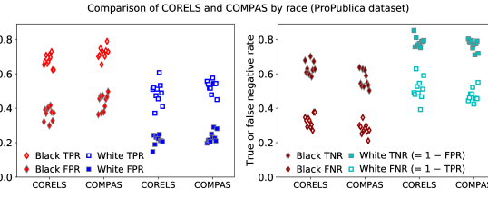
Figure 7: Comparison of TPR and FPR (left), as well as TNR and FNR (right), for different races in the ProPublica data set, for CORELS and COMPAS, across 10 cross-validation folds.

Figure 7 shows that CORELS and COMPAS perform similarly across both black and white individuals. Both algorithms have much higher true positive rates (TPR’s) and false positive rates (FPR’s) for blacks than whites (left), and higher true negative rates (TNR’s) and false negative rates (FNR’s) for whites than blacks (right). The fact that COMPAS has higher FPR’s for blacks and higher FNR’s for whites was a central observation motivating ProPublica’s claim that COMPAS is racially biased (Larson et al., 2016). The fact that CORELS’ models are so simple, with almost the same results as COMPAS, and contain only counts of past crimes, age, and gender, indicates possible explanations for the uneven predictions of both COMPAS and CORELS among blacks and whites. In particular, blacks evaluated within Broward County tend to be younger and have longer criminal histories within the data set, (on average, 4.4 crimes for blacks versus 2.6 crimes for whites) leading to higher FPR’s for blacks and higher FNR’s for whites. This aspect of the data could help to explain why ProPublica concluded that COMPAS was racially biased.

Similar observations have been reported for other datasets, namely that complex machine learning models do not have an advantage over simpler transparent models (Tollenaar and van der Heijden, 2013; Bushway, 2013; Zeng et al., 2017). There are many definitions of fairness, and it is not clear whether CORELS’ models are fair either, but it is much easier to debate about the fairness of a model when it is transparent. Additional fairness constraints or transparency constraints can be placed on CORELS’ models if desired, though one would need to edit our bounds (§3) and implementation (§5) to impose more constraints.

Regardless of whether COMPAS is racially biased (which our analysis does not indicate is necessarily true as long as criminal history and age are allowed to be considered as features), COMPAS may have many other fairness defects that might be considered serious. Many of COMPAS’s survey questions are direct inquiries about socioeconomic status. For instance, a sample COMPAS survey asks: “Is it easy to get drugs in your neighborhood?,” “How often do you have barely enough money to get by?,” “Do you frequently get jobs that don’t pay more than minimum wage?,” “How often have you moved in the last 12 months?” COMPAS’s survey questions also ask about events that were not caused by the person who is being evaluated, such as: “If you lived with both parents and they later separated, how old were you at the time?,” “Was one of your parents ever sent to jail or prison?,” “Was your mother ever arrested, that you know of?”

The fact that COMPAS requires over 130 questions to be answered, many of whose answers may not be verifiable, means that the computation of the COMPAS score is prone to errors. Even the Arnold Foundation’s “public-safety assessment” (PSA) score—which is completely transparent, and has only 9 factors—has been miscalculated in serious criminal trials, leading to a recent lawsuit (Westervelt, 2017). It is substantially more difficult to obtain the information required to calculate COMPAS scores than PSA scores (with over 14 times the number of survey questions). This significant discrepancy suggests that COMPAS scores are more fallible than PSA scores, as well as even simpler models, like those produced by CORELS. Some of these problems could be alleviated by using only data within electronic records that can be automatically calculated, instead of using information entered by hand and/or collected via subjective surveys.

The United States government pays Northpointe (now called Equivant) to use COMPAS. In light of our observations that CORELS is as accurate as COMPAS on a real-world data set where COMPAS is used in practice, CORELS predicts similarly to COMPAS for both blacks and whites, and CORELS’ models are completely transparent, it is not clear what value COMPAS scores possess. Our experiments also indicate that the proprietary survey data required to compute COMPAS scores has not boosted its prediction accuracy above that of transparent models in practice.

Risk predictions are important for the integrity of the judicial system; judges cannot be expected to keep entire databases in their heads to calculate risks, whereas models (when used correctly) can help to ensure equity. Risk prediction models also have the potential to heavily impact how efficient the judicial system is, in terms of bail and parole decisions; efficiency in this case means that dangerous individuals are not released, whereas non-dangerous individuals are granted bail or parole. High stakes decisions, such as these, are ideal applications for machine learning algorithms that produce transparent models from high dimensional data.

Currently, justice system data does not support highly accurate risk predictions, but current risk models are useful in practice, and these risk predictions will become more accurate as more and higher quality data are made available.

6.5 Comparison of CORELS to a Heuristic Model for Weapon Prediction

CORELS generates simple, accurate models for the task of weapon prediction, using the NYPD stop-and-frisk data set. Our approach offers a principled alternative to heuristic models proposed by Goel et al. (2016), who develop a series of regression models to analyze racial disparities in New York City’s stop-and-frisk policy for a related, larger data set. In particular, the authors arrive at a heuristic that they suggest could potentially help police officers more effectively decide when to frisk and/or search stopped individuals, i.e., when such interventions are likely to discover criminal possession of a weapon (CPW). Starting from a full regression model with 7,705 variables, the authors reduce this to a smaller model with 98 variables; from this, they keep three variables with the largest coefficients. This gives a heuristic model of the form ${ax+by+cz\geq T}$, where

$$x =\mathds{1}[stop~{}reason=suspicious~{}object]$$

$$y =\mathds{1}[stop~{}reason=suspicious~{}bulge]$$

$$z =\mathds{1}[additional~{}circumstances=sights~{}and~{}sounds~{}of~{}criminal~{}activity],$$

and $T$ is a threshold, such that the model predicts CPW when the threshold is met or exceeded. We focus on their approach that uses a single threshold, rather than precinct-specific thresholds. To increase ease-of-use, the authors round the coefficients to the nearest integers, which gives ${(a,b,c)=(3,1,1)}$; this constrains the threshold to take one of six values, ${T\in\{0,1,2,3,4,5\}}$. To employ this heuristic model in the field, “…officers simply need to add at most three small, positive integers …and check whether the sum exceeds a fixed threshold…” (Goel et al., 2016).

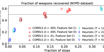
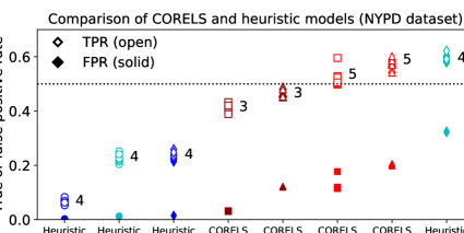
Figure 8: Weapon prediction with the NYPD stop-and-frisk data set, for various models learned by CORELS and the heuristic model by Goel et al. (2016), across 10 cross-validation folds. Note that the fraction of weapons recovered (top) is equal to the TPR (bottom, open markers). Markers above the dotted horizontal lines at the value 0.5 correspond to models that recover a majority of weapons (that are known in the data set). Top: Fraction of weapons recovered as a function of the fraction of stops where the individual was frisked and/or searched. In the legend, entries for CORELS (red markers) indicate the regularization parameter $({\lambda})$ and whether or not extra location features were used (“location”); entries for the heuristic model (blue markers) indicate the threshold value $(T)$. The results we report for the heuristic model are our reproduction of the results reported in Figure 9 by Goel et al. (2016) (first four open circles in that figure, from left to right; we exclude the trivial open circle showing 100% of weapons recovered at 100% of stops, obtained by setting the threshold at 0). Bottom: Comparison of TPR (open markers) and FPR (solid markers) for various CORELS and heuristic models. Models are sorted left-to-right by TPR. Markers and abbreviated horizontal tick labels correspond to the legend in the top figure. Numbers in the plot label model size; there was no variation in model size across folds, except for a single fold for CORELS (${{\lambda}=0.005}$, Feature Set C), which found a model of size 6.

Figure 8 directly compares various models learned by CORELS to the heuristic models, using the same data set as Goel et al. (2016) and 10-fold cross-validation. Recall that we train on resampled data to correct for class imbalance; we evaluate with respect to test sets that have been formed without resampling. For CORELS, the models correspond to the rule lists illustrated in Figure 6 from Section 6.3, and Figures 21 and 22 in Appendix F, we consider both Feature Sets C and D and both regularization parameters ${{\lambda}=0.005}$ and 0.01. The top panel plots the fraction of weapons recovered as a function of the fraction of stops where the individual was frisked and/or searched. Goel et al. (2016) target models that efficiently recover a majority of weapons (while also minimizing racial disparities, which we do not address here). Interestingly, the models learned by CORELS span a significant region that is not available to the heuristic model, which would require larger or non-integer parameters to access the region. The region is possibly desirable, since it includes models (${{\lambda}=0.005}$, bright red) that recover a majority (${\geq 50\%}$) of weapons (that are known in the data set). More generally, CORELS’ models all recover at least ${40\%}$ of weapons on average, i.e., more weapons than any of the heuristic models with ${T\geq 2}$, which recover less than 25% of weapons on average. At the same time, CORELS’ models all require well under 25% of stops—significantly less than the heuristic model with ${T=1}$, which requires over 30% of stops to recover a fraction of weapons comparable to the CORELS model that recovers the most weapons.

The bottom panel in Figure 8 plots both TPR and FPR and labels model size, for each of the models in the top panel. For the heuristic, we define model size as the number of model parameters; for CORELS, we use the number of rules in the rule list, which is equal to the number of leaves when we view a rule list as a decision tree. The heuristic models all have 4 parameters, while the different CORELS models have either 3 or approximately 5 rules. CORELS’ models are thus approximately as small, interpretable, and transparent as the heuristic models; furthermore, their predictions are straightforward to compute, without even requiring arithmetic.

6.6 Predictive Performance and Model Size for CORELS and Other Algorithms

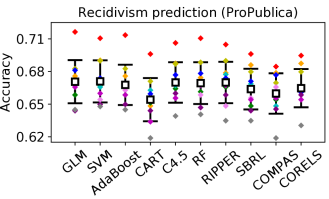
Figure 9: Two-year recidivism prediction for the ProPublica COMPAS data set. Comparison of CORELS and a panel of nine other algorithms: logistic regression (GLM), support vector machines (SVM), AdaBoost, CART, C4.5, random forests (RF), RIPPER, scalable Bayesian rule lists (SBRL), and COMPAS. For CORELS, we use regularization parameter ${{\lambda}=0.005}$.

We ran a 10-fold cross validation experiment using CORELS and eight other algorithms: logistic regression, support vector machines (SVM), AdaBoost, CART, C4.5, random forest (RF), RIPPER, and scalable Bayesian rule lists (SBRL). We use standard R packages, with default parameter settings, for the first seven algorithms. We use the same antecedent sets as input to the two rule list learning algorithms, CORELS and SBRL; for the other algorithms, the inputs are binary feature sets corresponding to the single clause antecedents in the aforementioned antecedent sets (see Appendix E).

Figure 9 shows that for the ProPublica data set, there were no statistically significant differences in test accuracies across algorithms, the difference between folds was far larger than the difference between algorithms. These algorithms also all perform similarly to the black box COMPAS algorithm. Figure 10 shows that for the NYCLU data set, logistic regression, SVM, and AdaBoost have the highest TPR’s and also the highest FPR’s; we show TPR and FPR due to class imbalance. For this problem, CORELS obtains an intermediate TPR, compared to other algorithms, while achieving a relatively low FPR. We conclude that CORELS produces models whose predictive performance is comparable to or better than those found via other algorithms.

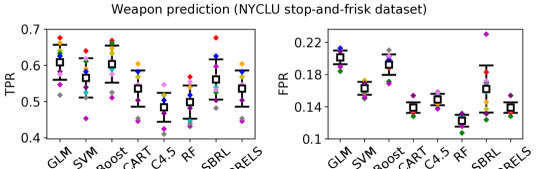
Figure 10: TPR (left) and FPR (right) for the test set, for CORELS and a panel of seven other algorithms, for the weapon prediction problem with the NYCLU stop-and-frisk data set. Means (white squares), standard deviations (error bars), and values (colors correspond to folds), for 10-fold cross-validation experiments. For CORELS, we use ${{\lambda}=0.01}$. Note that we were unable to execute RIPPER for the NYCLU problem.

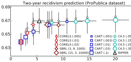
Figure 11: Training and test accuracy as a function of model size, across different methods, for two-year recidivism prediction with the ProPublica COMPAS data set. In the legend, numbers in parentheses are algorithm parameters that we vary for CORELS (${\lambda}$), CART ($cp$), C4.5 ($C$), and SBRL ($\eta$, $\lambda$, $i$), where $i$ is the number of iterations. Legend markers and error bars indicate means and standard deviations, respectively, across cross-validation folds. Small circles mark training accuracy means. None of the models exhibit significant overfitting; mean training accuracy never exceeds mean test accuracy by more than about 0.01.

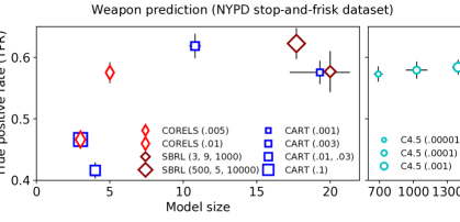
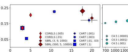
Figure 25: TPR (top) and FPR (bottom) for the test set, as a function of model size, across different methods, for weapon prediction with the NYPD stop-and-frisk data set (Feature Set D). In the legend, numbers in parentheses are algorithm parameters, as in Figure 12. Legend markers and error bars indicate means and standard deviations, respectively, across cross-validation folds. C4.5 finds large models for all tested parameters.

Figures 11 and 12 summarize differences in predictive performance and model size for CORELS and other tree (CART, C4.5) and rule list (RIPPER, SBRL) learning algorithms. Here, we vary different algorithm parameters, and increase the number of iterations for SBRL to 10,000. For two-year recidivism prediction with the ProPublica data set (Figure 11), we plot both training and test accuracy, as a function of the number of leaves in the learned model. Due to class imbalance for the weapon prediction problem with the NYCLU stop-and-frisk data set (Figure 12), we plot both true positive rate (TPR) and false positive rate (FPR), again as a function of the number of leaves. For both problems, CORELS can learn short rule lists without sacrificing predictive performance. For listings of example optimal rule lists that correspond to the results for CORELS summarized here, see Appendix F. Also see Figure 25 in Appendix G; it uses the larger NYPD data set and is similar to Figure 12.

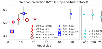
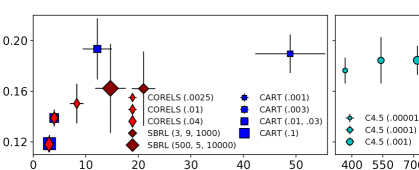
Figure 12: TPR (top) and FPR (bottom) for the test set, as a function of model size, across different methods, for weapon prediction with the NYCLU stop-and-frisk data set. In the legend, numbers in parentheses are algorithm parameters, as in Figure 11. Legend markers and error bars indicate means and standard deviations, respectively, across cross-validation folds. C4.5 finds large models for all tested parameters.

In Figure 4, we used CORELS to identify short rule lists, depending on only three features—age, prior convictions, and sex—that achieve test accuracy comparable to COMPAS (Figure 9, also see Angelino et al., 2017). If we restrict CORELS to search the space of rule lists formed from only age and prior convictions (${{\lambda}=0.005}$), the optimal rule lists it finds achieve test accuracy that is again comparable to COMPAS. CORELS identifies the same rule list across all 10 folds of 10-fold cross-validation experiments (Figure 13). In work subsequent to ours (Angelino et al., 2017), Dressel and Farid (2018) confirmed this result, in the sense that they used logistic regression to construct a linear classifier with age and prior convictions, and also achieved similar accuracy to COMPAS. However, computing a logistic regression model requires multiplication and addition, and their model cannot easily be computed, in the sense that it requires a calculator (and thus is potentially error-prone). Our rule lists require no such computation.

if $(priors>3)$ then predict $yes$

else if $(age<25){\bf~{}and~{}}(priors=2-3)$ then predict $yes$

else predict $no$

Figure 13: When restricted to two features (age, priors), CORELS (${{\lambda}=0.005}$) finds the same rule list across 10 cross-validation folds.

6.7 CORELS Execution Traces, for Different Regularization Parameters

In this section, we illustrate several views of CORELS execution traces, for the NYCLU stop-and-frisk data set with ${M=46}$ antecedents, for the same three regularization parameters (${{\lambda}=.04,.01,.025}$) as in Figure 12.

CORELS with different regularization parameters (NYCLU stop-and-frisk data set)
Total Time to Max evaluated Optimal $\lambda$ time (s) optimum (s) prefix length prefix length .04  .61 (.03) .002 (.001) 6 2 .01 70 (6) .008 (.002) 11 3 .0025 1600 (100) 56 (74) 16-17 6-10 Lower bound Total queue Max queue $\lambda$   evaluations ($\times 10^{6}$)   insertions ($\times 10^{3}$)   size ($\times 10^{3}$) .04  .070 (.004) 2.2 (.1)  .9 (.1) .01 7.5 (.6) 210 (20) 130 (10) .0025 150 (10) 4400 (300) 2500 (170)

Table 3: Summary of CORELS executions, for the NYCLU stop-and-frisk data set (${M=46}$), for same three regularization parameter (${\lambda}$) values as in Figure 12. The columns report the total execution time, time to optimum, maximum evaluated prefix length, optimal prefix length, number of times we completely evaluate a prefix $d_{p}$’s lower bound $b(d_{p},\mathbf{x},\mathbf{y})$, total number of queue insertions (this number is equal to the number of cache insertions), and the maximum queue size. For prefix lengths, we report single values or ranges corresponding to the minimum and maximum observed values; in the other columns, we report means (and standard deviations) over 10 cross-validation folds. See also Figures 14 and 15.

Table 3 summarizes execution traces across all 10 cross-validation folds. For each value of ${\lambda}$, CORELS achieves the optimum in a small fraction of the total execution time. As ${\lambda}$ decreases, these times increase because the search problems become more difficult, as is summarized by the observation that CORELS must evaluate longer prefixes; consequently, our data structures grow in size. We report the total number of elements inserted into the queue and the maximum queue size; recall from §5 that the queue elements correspond to the trie’s leaves, and that the symmetry-aware map elements correspond to the trie’s nodes.

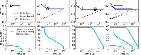
Figure 14: Example executions of CORELS, for the NYCLU stop-and-frisk data set (${M=46}$). See also Table 3 and Figure 15. Top: Objective value (solid line) and lower bound (dashed line) for CORELS, as a function of wall clock time (log scale). Numbered points along the trace of the objective value indicate when the length of the best known rule list changes and are labeled by the new length. For each value of ${\lambda}$, a star marks the optimum objective value and time at which it was achieved. Bottom: $\lfloor\log_{10}\Gamma({R^{c}},Q)\rfloor$, as a function of wall clock time (log scale), where $\Gamma({R^{c}},Q)$ is the upper bound on remaining search space size (Theorem 7). Rightmost panels: For visual comparison, we overlay the execution traces from the panels to the left, for the three different values of ${\lambda}$.

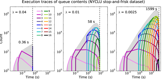
Figure 15: Summary of CORELS’ logical queue, for the NYCLU stop-and-frisk data set (${M=46}$), for same three regularization parameters as in Figure 12 and Table 3. Solid lines plot the numbers of prefixes in the logical queue (log scale), colored by length (legend), as a function of wall clock time (log scale). All plots are generated using a single, representative cross-validation training set. For each execution, the gray shading fills in the area beneath the total number of queue elements, i.e., the sum over all lengths; we also annotate the total time in seconds, marked with a dashed vertical line.

The upper panels in Figure 14 plot example execution traces, from a single cross-validation fold, of both the current best objective value ${R^{c}}$ and the lower bound $b(d_{p},\mathbf{x},\mathbf{y})$ of the prefix $d_{p}$ being evaluated. These plots illustrate that CORELS certifies optimality when the lower bound matches the objective value. The lower panels in Figure 14 plot corresponding traces of an upper bound on the size of the remaining search space (Theorem 7), and illustrate that as ${\lambda}$ decreases, it becomes more difficult to eliminate regions of the search space. For Figure 14, we dynamically and incrementally calculate $\lfloor\log_{10}\Gamma({R^{c}},Q)\rfloor$, which adds some computational overhead; we do not calculate this elsewhere unless noted.

Figure 15 visualizes the elements in CORELS’ logical queue, for each of the executions in Figure 14. Recall from §5.5 that the logical queue corresponds to elements in the (physical) queue that have not been garbage collected from the trie; these are prefixes that CORELS has already evaluated and whose children the algorithm plans to evaluate next. As an execution progresses, longer prefixes are placed in the queue; as ${\lambda}$ decreases, the algorithm must spend more time evaluating longer and longer prefixes.

6.8 Efficacy of CORELS Algorithm Optimizations

Per-component performance improvement (ProPublica data set)
Total time Slow- Time to Max evaluated Algorithm variant (min) down optimum (s) prefix length CORELS  .98 (.6) —   1 (1) 5 No priority queue (BFS) 1.03 (.6) 1.1$\times$   2 (4) 5 No support bounds  1.5 (.9) 1.5$\times$   1 (2) 5 No lookahead bound  12.3 (6.2) 13.3$\times$   1 (1) 6 No symmetry-aware map    9.1 (6.4) 8.4$\times$   2 (3) 5 No equivalent points bound* $>$130 (2.6) $>$180$\times$ $>$1400 (2000) $\geq$11 Lower bound Total queue Max queue Algorithm variant evaluations ($\times 10^{6}$) insertions ($\times 10^{6}$)   size ($\times 10^{6}$) CORELS 26 (15) .29 (.2) .24 (.1) No priority queue (BFS) 27 (16) .33 (.2) .20 (.1) No support bounds 42 (25) .40 (.2) .33 (.2) No lookahead bound 320 (160) 3.6 (1.8) 3.0 (1.5) No symmetry-aware map 250 (180) 2.5 (1.7) 2.4 (1.7) No equivalent points bound* $>$940 (5) $>$510 (1.1) $>$500 (1.2)

Table 4: Per-component performance improvement, for the ProPublica data set (${{\lambda}=0.005}$, ${M=122}$). The columns report the total execution time, time to optimum, maximum evaluated prefix length, number of times we completely evaluate a prefix $d_{p}$’s lower bound $b(d_{p},\mathbf{x},\mathbf{y})$, total number of queue insertions (which is equal to the number of cache insertions), and maximum logical queue size. The first row shows CORELS; subsequent rows show variants that each remove a specific implementation optimization or bound. (We are not measuring the cumulative effects of removing a sequence of components.) All rows represent complete executions that certify optimality, except those labeled ‘No equivalent points bound,’ for which each execution was terminated due to memory constraints, once the size of the cache reached ${5\times 10^{8}}$ elements, after consuming $\sim$250GB RAM. In all but the final row and column, we report means (and standard deviations) over 10 cross-validation folds. We also report the mean slowdown in total execution time, with respect to CORELS. In the final row, we report the mean (and standard deviation) of the incomplete execution time and corresponding slowdown, and a lower bound on the mean time to optimum; in the remaining fields, we report minimum values across folds. See also Figure 16.
* Only 7 out of 10 folds achieve the optimum before being terminated.

This section examines the efficacy of each of our bounds and data structure optimizations. We remove a single bound or data structure optimization from our final implementation and measure how the performance of our algorithm changes. We examine these performance traces on both the NYCLU and the ProPublica data sets, and highlight the result that on different problems, the relative performance improvements of our optimizations can vary.

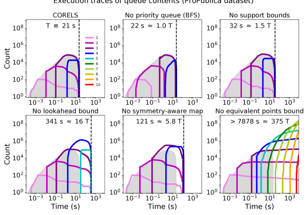
Figure 16: Summary of the logical queue’s contents, for full CORELS (top left) and five variants that each remove a specific implementation optimization or bound, for the ProPublica data set (${{\lambda}=0.005}$, ${M=122}$). See also Table 4. Solid lines plot the numbers of prefixes in the logical queue (log scale), colored by length (legend), as a function of wall clock time (log scale). All plots are generated using a single, representative cross-validation training set. The gray shading fills in the area beneath the total number of queue elements for CORELS, i.e., the sum over all lengths in the top left figure. For comparison, we replicate the same gray region in the other five subfigures. For each execution, we indicate the total time in seconds, relative to the full CORELS implementation (T = 21 s), and with a dashed vertical line. The execution without the equivalent points bound (bottom right) is incomplete.

Table 4 provides summary statistics for experiments using the full CORELS implementation (first row) and five variants (subsequent rows) that each remove a specific optimization: (1) Instead of a priority queue (§5.2) ordered by the objective lower bound, we use a queue that implements breadth-first search (BFS). (2) We remove checks that would trigger pruning via our lower bounds on antecedent support (Theorem 10) and accurate antecedent support (Theorem 11). (3) We remove the effect of our lookahead bound (Lemma 2), which otherwise tightens the objective lower bound by an amount equal to the regularization parameter ${\lambda}$. (4) We disable the symmetry-aware map (§5.3), our data structure that enables pruning triggered by the permutation bound (Corollary 16). (5) We do not identify sets of equivalent points, which we otherwise use to tighten the objective lower bound via the equivalent points bound (Theorem 20).

Per-component performance improvement (NYCLU stop-and-frisk data set)
Total Slow- Time to Max evaluated Algorithm variant time (min) down optimum ($\mu$s) prefix length CORELS    1.1 (.1) — 8.9 (.1) 11 No priority queue (BFS)    2.2 (.2) 2.0$\times$ 110 (10) 11 No support bounds    1.2 (.1) 1.1$\times$ 8.8 (.8) 11 No lookahead bound    1.7 (.2) 1.6$\times$  7.3 (1.8) 11-12 No symmetry-aware map $>$ 73 (5) $>$ 68$\times$ $>$ 7.6 (.4) $>$ 10 No equivalent points bound      4 (.3) 3.8$\times$ 6.4 (.9) 14 Lower bound Total queue Max queue Algorithm variant evaluations ($\times 10^{6}$) insertions ($\times 10^{5}$)   size ($\times 10^{5}$) CORELS  7 (1) 2.0 (.2) 1.3 (.1) No priority queue (BFS) 14 (1) 4.1 (.4) 1.4 (.1) No support bounds  8 (1) 2.1 (.2) 1.3 (.1) No lookahead bound 11 (1) 3.2 (.3) 2.1 (.2) No symmetry-aware map $>$ 390 (40) $>$ 1000 (0) $>$ 900 (10) No equivalent points bound 33 (2) 9.4 (.7) 6.0 (.4)

Table 5: Per-component performance improvement, as in Table 4, for the NYCLU stop-and-frisk data set (${{\lambda}=0.01}$, ${M=46}$). All rows except those labeled ‘No symmetry-aware map’ represent complete executions. A single fold running without a symmetry-aware map required over 2 days to complete, so in order to run all 10 folds above, we terminated execution after the prefix tree (§5.1) reached $10^{8}$ nodes. See Table 4 for a detailed caption, and also Figure 17.

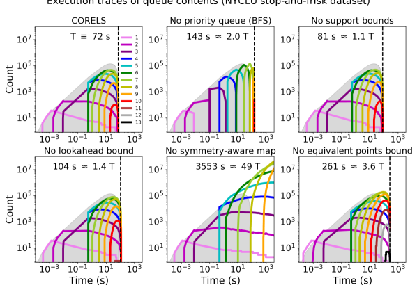
Figure 17: Summary of the logical queue’s contents, for full CORELS (top left) and five variants that each remove a specific implementation optimization or bound, for the NYCLU stop-and-frisk data set (${{\lambda}=0.01}$, ${M=46}$), as in Table 5. The execution without the symmetry-aware map (bottom center) is incomplete. See Figure 16 for a detailed caption.

Removing any single optimization increases total execution time, by varying amounts across these optimizations. Similar to our experiments in §6.7, we always encounter the optimal rule list in far less time than it takes to certify optimality. As in Table 3, we report metrics that are all proxies for how much computational work our algorithm must perform; these metrics thus scale with the overall slowdown with respect to CORELS execution time (Table 4, first column).

Figure 16 visualizes execution traces of the elements in CORELS’ logical queue, similar to Figure 15, for a single, representative cross-validation fold. Panels correspond to different removed optimizations, as in Table 4. These plots demonstrate that our optimizations reduce the number of evaluated prefixes and are especially effective at limiting the number of longer evaluated prefixes. For the ProPublica data set, the most important optimization is the equivalent points bound—without it, we place prefixes of at least length 10 in our queue, and must terminate these executions before they are complete. In contrast, CORELS and most other variants evaluate only prefixes up to at most length 5, except for the variant without the lookahead bound, which evaluates prefixes up to length 6.

Table 5 and Figure 17 summarize an analogous set of experiments for the NYCLU data set. Note that while the equivalent points bound proved to be the most important optimization for the ProPublica data set, the symmetry-aware map is the crucial optimization for the NYCLU data set.

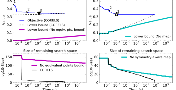
Figure 18: Execution progress of CORELS and selected variants, for the ProPublica (${{\lambda}=0.005}$, ${M=122}$) (left) and NYCLU (${{\lambda}=0.01}$, ${M=46}$) (right) data sets. Top: Objective value (thin solid lines) and lower bound (dashed lines) for CORELS, as a function of wall clock time (log scale). Numbered points along the trace of the objective value indicate when the length of the best known rule list changes, and are labeled by the new length. CORELS quickly achieves the optimal value (star markers), and certifies optimality when the lower bound matches the objective value. On the left, a separate and significantly longer execution of CORELS without the equivalent points (Theorem 20) bound remains far from complete, and its lower bound (thick solid line) far from the optimum. On the right, a separate execution of CORELS without the permutation bound (Corollary 16), and thus the symmetry-aware map, requires orders of magnitude more time to complete. Bottom: $\lfloor\log_{10}\Gamma({R^{c}},Q)\rfloor$, as a function of wall clock time (log scale), where $\Gamma({R^{c}},Q)$ is the upper bound (13) on remaining search space size (Theorem 7). For these problems, the equivalent points (left) and permutation (right) bounds are responsible for the ability of CORELS to quickly eliminate most of the search space (thin solid lines); the remaining search space decays much more slowly without these bounds (thick solid lines).

Finally, Figure 18 highlights the most significant algorithm optimizations for our prediction problems: the equivalent points bound for the ProPublica data set (left) and the symmetry-aware map for the NYCLU data set (right). For CORELS (thin lines) with the ProPublica recidivism data set (left), the objective drops quickly, achieving the optimal value within a second. CORELS certifies optimality in about a minute—the objective lower bound steadily converges to the optimal objective (top) as the search space shrinks (bottom). As in Figure 14, we dynamically and incrementally calculate $\lfloor\log_{10}\Gamma({R^{c}},Q)\rfloor$, where $\Gamma({R^{c}},Q)$ is the upper bound (13) on remaining search space size (Theorem 7); this adds some computational overhead. In the same plots (left), we additionally highlight a separate execution of CORELS without the equivalent points bound (Theorem 20) (thick lines). After more than 2 hours, the execution is still far from complete; in particular, the lower bound is far from the optimum objective value (top) and much of the search space remains unexplored (bottom). For the NYCLU stop-and-frisk data set (right), CORELS achieves the optimum objective in well under a second, and certifies optimality in a little over a minute. CORELS without the permutation bound (Corollary 16), and thus the symmetry-aware map, requires more than an hour, i.e., orders of magnitude more time, to complete (thick lines).

6.9 Algorithmic Speedup

Algorithmic	Max evaluated	Lower bound	Predicted	runtime
approach	prefix length	evaluations
CORELS	5	$2.8\times 10^{7}$	$36$ seconds
Brute force	5	$2.5\times 10^{10}$	$9.0$ hours	$\approx 3.3\times 10^{4}$ s
Brute force	10	$5.0\times 10^{20}$	$21\times 10^{6}$ years	$\approx 6.5\times 10^{14}$ s
CORELS (1984)	5	$2.8\times 10^{7}$	$13.5$ days	$\approx 1.2\times 10^{6}$ s

Table 6: Algorithmic speedup for the ProPublica data set (${{\lambda}=0.005}$, ${M=122}$). Solving this problem using brute force is impractical due to the inability to explore rule lists of reasonable lengths. Removing only the equivalent points bound requires exploring prefixes of up to length 10 (see Table 4), a clearly intractable problem. Even with all of our improvements, however, it is only recently that processors have been fast enough for this type of discrete optimization algorithm to succeed.

Table 6 shows the overall speedup of CORELS compared to a naïve implementation and demonstrates the infeasibility of running our algorithm 30 years ago. Consider an execution of CORELS for the ProPublica data set, with ${M=122}$ antecedents, that evaluates prefixes up to length 5 in order to certify optimality (Table 4). A brute force implementation that naïvely considers all prefixes of up to length 5 would evaluate ${2.5\times 10^{10}}$ prefixes. As shown in Figure 4, the optimal rule list has prefix length 3, thus the brute force algorithm would identify the optimal rule list. However, for this approach to certify optimality, it would have to consider far longer prefixes. Without our equivalent points bound, but with all of our other optimizations, we evaluate prefixes up to at least length 10 (see Table 4 and Figure 16)—thus a brute force algorithm would have to evaluate prefixes of length 10 or longer. Naïvely evaluating all prefixes up to length 10 would require looking at ${5.0\times 10^{20}}$ different prefixes.

However, CORELS examines only 28 million prefixes in total—a reduction of 893$\times$ compared to examining all prefixes up to length 5 and a reduction of ${1.8\times 10^{13}}$ for the case of length 10. On a laptop, we require about 1.3 $\mu$s to evaluate a single prefix (given by dividing the number of lower bound evaluations by the total time in Table 4). Our runtime is only about 36 seconds, but the naïve solutions of examining all prefixes up to lengths 5 and 10 would take 9 hours and 21 million years, respectively. It is clear that brute force would not scale to larger problems.

We compare our current computing circumstances to those of 1984, the year when CART was published. Moore’s law holds that computing power doubled every 18 months from 1984 to 2006. This is a period of 264 months, which means computing power has gone up by at least a factor of 32,000 since 1984. Thus, even with our algorithmic and data structural improvements, CORELS would have required about 13.5 days in 1984—an unreasonable amount of time. Our advances are meaningful only because we can run them on a modern system. Combining our algorithmic improvements with the increase in modern processor speeds, our algorithm runs more than $10^{13}$ times faster than a naïve implementation would have in 1984. This helps explain why neither our algorithm, nor other branch-and-bound variants, had been developed before now.

7 Summary and Future Work on Bounds

Here, we highlight our most significant bounds, as well as directions for future work based on bounds that we have yet to leverage in practice.

In empirical studies, we found our equivalent support (§3.10, Theorem 15) and equivalent points (§3.14, Theorem 20) bounds to yield the most significant improvements in algorithm performance. In fact, they sometimes proved critical for finding solutions and proving optimality, even on small problems.

Accordingly, we would hope that our similar support bound (§3.13, Theorem 18) could be useful; understanding how to efficiently exploit this result in practice represents an important direction for future work. In particular, this type of bound may lead to principled approximate variants of our approach.

We presented several sets of bounds in which at least one bound was strictly tighter than the other(s). For example, the lower bound on accurate antecedent support (Theorem 11) is strictly tighter than the lower bound on accurate support (Theorem 10). It might seem that we should only use this tighter bound, but in practice, we can use both—the looser bound can be checked before completing the calculation required to check the tighter bound. Similarly, the equivalent support bound (Theorem 15) is more general than the special case of the permutation bound (Corollary 16). We have implemented data structures, which we call symmetry-aware maps, to support both of these bounds, but have not yet identified an efficient approach for supporting the more general equivalent points bound. A good solution may be related to the challenge of designing an efficient data structure to support the similar support bound.

We also presented results on antecedent rejection that unify our understanding of our lower (§3.7) and upper bounds (§3.8) on antecedent support. In a preliminary implementation (not described here), we experimented with special data structures to support the direct use of our observation that antecedent rejection propagates (§3.9, Theorem 12). We leave the design of efficient data structures for this task as future work.

During execution, we find it useful to calculate an upper bound on the size of the remaining search space—e.g., via Theorem 7, or the looser Proposition 9, which incurs less computational overhead—since these provide meaningful information about algorithm progress and allow us to estimate the remaining execution time. As we illustrated in Section 6.8, these calculations also help us qualify the impact of different algorithmic bounds, e.g., by comparing executions that keep or remove bounds.

When our algorithm terminates, it outputs an optimal solution of the training optimization problem, with a certificate of optimality. On a practical note, our approach can also provide useful results even for incomplete executions. As shown earlier, we have empirically observed that our algorithm often identifies the optimal rule list very quickly, compared to the total time required to prove optimality, e.g., in seconds, versus minutes, respectively. Furthermore, our objective’s lower bounds allow us to place an upper bound on the size of the remaining search space, and provides guarantees on the quality of a solution output by an incomplete execution.

The order in which we evaluate prefixes can impact the rate at which we prune the search space, and thus the total runtime. We think that it is possible to design search policies that significantly improve performance.

8 Conclusion and More Possible Directions for Future Work

Finally, we would like to clarify some limitations of CORELS. As far as we can tell, CORELS is the current best algorithm for solving a specialized optimal decision tree problem. While our approach scales well to large numbers of observations, it could have difficulty proving optimality for problems with many possibly relevant features that are highly correlated, when large regions of the search space might be challenging to exclude.

CORELS is not designed for raw image processing or other problems where the features themselves are not interpretable. It could instead be used as a final classifier for image processing problems where the features were created beforehand; for instance, one could create classifiers for each part of an image, and use CORELS to create a final combined classifier. The notions of interpretability used in image classification tend to be completely different from those for structured data where each feature is separately meaningful (e.g., see Li et al., 2018). For structured data, decision trees, along with scoring systems, tend to be popular forms of transparent models. Scoring systems are sparse linear models with integer coefficients, and they can also be created from data (Ustun and Rudin, 2017, 2016).

In some of our experiments, CORELS produces a DNF formula by coincidence, but it might be possible to create a much simpler version of CORELS that only produces DNF formulae. This could build off previous algorithms for creating an optimal DNF formula (Rijnbeek and Kors, 2010; Wang et al., 2016, 2017).

CORELS does not automatically rank the subgroups in order of the likelihood of a positive outcome; doing so would require an algorithm such as Falling Rule Lists (Wang and Rudin, 2015a; Chen and Rudin, 2018), which forces the estimated probabilities to decrease along the list. Furthermore, while CORELS does not technically produce estimates of ${\mathbb{P}(Y=1\,|\,x)}$, one could form such an estimate by computing the empirical proportion ${\hat{\mathbb{P}}(Y=1\,|\,x\textrm{ obeys }p_{k})}$ for each antecedent $p_{k}$. CORELS is also not designed to assist with causal inference applications, since it does not estimate the effect of a treatment via the conditional difference ${\mathbb{P}(Y=1\,|\,\textrm{treatment}=}$ ${\textrm{True},x)}$ $-$ ${\mathbb{P}(Y=1\,|\,\textrm{treatment}=}$ ${\textrm{False},x)}$. Alternative algorithms that estimate conditional differences with interpretable rule lists include Causal Falling Rule Lists (Wang and Rudin, 2015b), Cost-Effective Interpretable Treatment Regimes (CITR) (Lakkaraju and Rudin, 2017), and an approach by Zhang et al. (2015) for constructing interpretable and parsimonious treatment regimes. Alternatively, one could use a complex machine learning model to predict outcomes for the treatment group and a separate complex model for the control group that would allow counterfactuals to be estimated for each observation; from there, CORELS could be applied to produce a transparent model for personalized treatment effects. A similar approach to this was taken by Goh and Rudin (2018), who use CORELS to understand a black box causal model.

CORELS could be adapted to handle cost-sensitive learning or weighted regularization. This would require creating more general versions of our theorems, which would be an extension of this work.

While CORELS does not directly handle continuous variables, we have found that it is not difficult in practice to construct a rule set that is sufficient for creating a useful model. It may be possible to use techniques such as Fast Boxes (Goh and Rudin, 2014) to discover useful and interpretable rules for continuous data that can be used within CORELS.

An interesting direction for future research would be to create a hybrid interpretable/ black box model in the style of Wang (2018), where the rule list would eliminate large parts of the space away from the decision boundary, and the observations that remain are evaluated by a black box model rather than a default rule.

Lastly, CORELS does not create generic single-variable-split decision trees. CORELS optimizes over rule lists, which are one-sided decision trees; in our setting, the leaves of these ‘trees’ are conjunctions. It may be possible to generalize ideas from our approach to handle generic decision trees, which could be an interesting project for future work. There are more symmetries to handle in that case, since there would be many equivalent decision trees, leading to challenges in developing symmetry-aware data structures.

Acknowledgments

E.A. conducted most of this work while supported by the Miller Institute for Basic Research in Science, University of California, Berkeley, and hosted by Prof. M.I. Jordan at RISELab. C.D.R. is supported in part by MIT-Lincoln Labs and the National Science Foundation under IIS-1053407. E.A. would like to thank E. Jonas, E. Kohler, and S. Tu for early implementation guidance, A. D’Amour for pointing out the work by Goel et al. (2016), V. Kanade, S. McCurdy, J. Schleier-Smith and E. Thewalt for helpful conversations, and members of RISELab, SAIL, and the UC Berkeley Database Group for their support and feedback. We thank H. Yang and B. Letham for sharing advice and code for processing data and mining rules, B. Coker for his critical advice on using the ProPublica COMPAS data set, as well as V. Kaxiras and A. Saligrama for their recent contributions to our implementation and for creating the CORELS website. We are very grateful to our editor and anonymous reviewers.

A Excessive Antecedent Support

Theorem 21 (Upper bound on antecedent support)

Let ${d^{*}=(d_{p},\delta_{p},q_{0},K)}$ be any optimal rule list with objective $R^{*}$, i.e., ${d^{*}\in\operatorname*{argmin}_{d}R({d},\mathbf{x},\mathbf{y})}$, and let ${d_{p}=(p_{1},\dots,p_{k-1},}$ ${p_{k},\dots,p_{K})}$ be its prefix. For each ${k\leq K}$, antecedent $p_{k}$ in $d_{p}$ has support less than or equal to the fraction of all data not captured by preceding antecedents, by an amount greater than the regularization parameter ${\lambda}$:

$$\textnormal{supp}(p_{k},\mathbf{x}\,|\,d_{p})\leq 1-\textnormal{supp}(d_{p}^{k-1},\mathbf{x})-{\lambda},$$ (37)

where ${d_{p}^{k-1}=(p_{1},\dots,p_{k-1})}$. For the last antecedent, i.e., when ${p_{k}=p_{K}}$, equality implies that there also exists a shorter optimal rule list ${{d}^{\prime}=(d_{p}^{K-1},\delta_{p}^{\prime},q_{0}^{\prime},K-1)\in}$ ${\operatorname*{argmin}_{d}R({d},\mathbf{x},\mathbf{y})}$.

Proof  First, we focus on the last antecedent $p_{K+1}$ in a rule list ${d}^{\prime}$. Let ${{d}=(d_{p},\delta_{p},q_{0},K)}$ be a rule list with prefix ${d_{p}=(p_{1},\dots,p_{K})}$ and objective ${R({d},\mathbf{x},\mathbf{y})\geq R^{*}}$, where ${R^{*}\equiv}$ ${\min_{{D}}R({D},\mathbf{x},\mathbf{y})}$ is the optimal objective. Let ${{d}^{\prime}=(d_{p}^{\prime},\delta_{p}^{\prime},q_{0}^{\prime},K+1)}$ be a rule list whose prefix ${d_{p}^{\prime}=(p_{1},\dots,p_{K},p_{K+1})}$ starts with $d_{p}$ and ends with a new antecedent $p_{K+1}$. Suppose $p_{K+1}$ in the context of $d_{p}^{\prime}$ captures nearly all data not captured by $d_{p}$, except for a fraction $\epsilon$ upper bounded by the regularization parameter ${\lambda}$:

$$1-\textnormal{supp}(d_{p},\mathbf{x})-\textnormal{supp}(p_{K+1},\mathbf{x}\,|\,d_{p}^{\prime})\equiv\epsilon\leq{\lambda}.$$

Since $d_{p}^{\prime}$ starts with $d_{p}$, its prefix misclassification error is at least as great; the only discrepancy between the misclassification errors of ${d}$ and ${d}^{\prime}$ can come from the difference between the support of the set of data not captured by $d_{p}$ and the support of $p_{K+1}$:

$$|\ell({d}^{\prime},\mathbf{x},\mathbf{y})-\ell({d},\mathbf{x},\mathbf{y})|\leq 1-\textnormal{supp}(d_{p},\mathbf{x})-\textnormal{supp}(p_{K+1},\mathbf{x}\,|\,d_{p}^{\prime})=\epsilon.$$

The best outcome for ${d}^{\prime}$ would occur if its misclassification error were smaller than that of ${d}$ by $\epsilon$, therefore

$$R({d}^{\prime},\mathbf{x},\mathbf{y}) =\ell({d}^{\prime},\mathbf{x},\mathbf{y})+{\lambda}(K+1)$$

$$\geq\ell({d},\mathbf{x},\mathbf{y})-\epsilon+{\lambda}(K+1)=R({d},\mathbf{x},\mathbf{y})-\epsilon+{\lambda}\geq R({d},\mathbf{x},\mathbf{y})\geq R^{*}.$$

${d}^{\prime}$ is an optimal rule list, i.e., ${{d}^{\prime}\in\operatorname*{argmin}_{{D}}R({D},\mathbf{x},y)}$, if and only if ${R({d}^{\prime},\mathbf{x},\mathbf{y})=R({d},\mathbf{x},\mathbf{y})=}$ ${R^{*}}$, which requires ${\epsilon={\lambda}}$. Otherwise, ${\epsilon<{\lambda}}$, in which case

$$R({d}^{\prime},\mathbf{x},\mathbf{y})\geq R({d},\mathbf{x},\mathbf{y})-\epsilon+{\lambda}>R({d},\mathbf{x},\mathbf{y})\geq R^{*},$$

therefore ${d}^{\prime}$ is not optimal, i.e., ${{d}^{\prime}\notin\operatorname*{argmin}_{{D}}R({D},\mathbf{x},\mathbf{y})}$. This demonstrates the desired result for ${k=K}$.

In the remainder, we prove the bound in (37) by contradiction, in the context of a rule list ${d}^{\prime\prime}$. Let ${d}$ and ${d}^{\prime}$ retain their definitions from above, thus as before, that the data not captured by $d_{p}^{\prime}$ has normalized support ${\epsilon\leq{\lambda}}$, i.e.,

$$1-\textnormal{supp}(d_{p}^{\prime},\mathbf{x})=1-\textnormal{supp}(d_{p},\mathbf{x})-\textnormal{supp}(p_{K+1},\mathbf{x}\,|\,d_{p}^{\prime})=\epsilon\leq{\lambda}.$$

Thus for any rule list ${d}^{\prime\prime}$ whose prefix $d_{p}^{\prime\prime}=(p_{1},\dots,p_{K+1},\dots,p_{K^{\prime}})$ starts with $d_{p}^{\prime}$ and ends with one or more additional rules, each additional rule $p_{k}$ has support ${\textnormal{supp}(p_{k},\mathbf{x}\,|\,d_{p}^{\prime\prime})\leq}$ ${\epsilon\leq{\lambda}}$, for all ${k>K+1}$. By Theorem 10, all of the additional rules have insufficient support, therefore $d_{p}^{\prime\prime}$ cannot be optimal, i.e., ${{d}^{\prime\prime}\notin\operatorname*{argmin}_{{D}}R({D},\mathbf{x},\mathbf{y})}$.  

Similar to Theorem 10, our lower bound on antecedent support, we can apply Theorem 21 in the contexts of both constructing rule lists and rule mining (§3.1). Theorem 21 implies that if we only seek a single optimal rule list, then during branch-and-bound execution, we can prune a prefix if we ever add an antecedent with support too similar to the support of the set of data not captured by the preceding antecedents. One way to view this result is that if ${{d}=(d_{p},\delta_{p},q_{0},K)}$ and ${{d}^{\prime}=(d_{p}^{\prime},\delta_{p}^{\prime},q_{0}^{\prime},K+1)}$ are rule lists such that $d_{p}^{\prime}$ starts with $d_{p}$ and ends with an antecedent that captures all or nearly all data not captured by $d_{p}$, then the new rule in ${d}^{\prime}$ behaves similar to the default rule of ${d}$. As a result, the misclassification error of ${d}^{\prime}$ must be similar to that of ${d}$, and any reduction may not be sufficient to offset the penalty for longer prefixes.

Proposition 22 (Excessive antecedent support propagates)

Define $\phi(d_{p})$ as in (19), and let ${d_{p}=(p_{1},\dots,p_{K})}$ be a prefix, such that its last antecedent $p_{K}$ has excessive support, i.e., the opposite of the bound in (37):

$$\textnormal{supp}(p_{K},\mathbf{x}\,|\,d_{p})>1-\textnormal{supp}(d_{p}^{K-1},\mathbf{x})-{\lambda},$$

where ${d_{p}^{K-1}=(p_{1},\dots,p_{K-1})}$. Let ${{D}=(D_{p},\Delta_{p},Q_{0},\kappa)}$ be any rule list with prefix ${D_{p}=}$ ${(P_{1},\dots,P_{\kappa})}$ such that $D_{p}$ starts with ${D_{p}^{K^{\prime}-1}=}$ ${(P_{1},\dots,P_{K^{\prime}-1})\in\phi(d_{p}^{K-1})}$ and ${P_{K^{\prime}}=p_{K}}$. It follows that $P_{K^{\prime}}$ has excessive support in prefix $D_{p}$, and furthermore, ${{D}\notin\operatorname*{argmin}_{{d}}R({d},\mathbf{x},\mathbf{y})}$.

Proof  Since ${D_{p}^{K^{\prime}}=(P_{1},\dots,P_{K^{\prime}})}$ contains all the antecedents in $d_{p}$, we have that

$$\textnormal{supp}(D_{p}^{K^{\prime}},\mathbf{x})\geq\textnormal{supp}(d_{p},\mathbf{x}).$$

Expanding these two terms gives

$$\textnormal{supp}(D_{p}^{K^{\prime}},\mathbf{x}) =\textnormal{supp}(D_{p}^{K^{\prime}-1},\mathbf{x})+\textnormal{supp}(P_{K^{\prime}},\mathbf{x}\,|\,D_{p})$$

$$\geq\textnormal{supp}(d_{p},\mathbf{x})=\textnormal{supp}(d_{p}^{K-1},\mathbf{x})+\textnormal{supp}(p_{K},\mathbf{x}\,|\,d_{p})>1-{\lambda}.$$

Rearranging gives

$$\textnormal{supp}(P_{K^{\prime}},\mathbf{x}\,|\,D_{p})>1-\textnormal{supp}(D_{p}^{K^{\prime}-1},\mathbf{x})-{\lambda},$$

thus $P_{K^{\prime}}$ has excessive support in $D_{p}$. By Theorem 21, ${{D}\notin\operatorname*{argmin}_{{d}}R({d},\mathbf{x},\mathbf{y})}$.  

B Proof of Theorem 15 (Equivalent Support Bound)

We begin by defining four related rule lists. First, let ${{d}=(d_{p},\delta_{p},q_{0},K)}$ be a rule list with prefix ${d_{p}=(p_{1},\dots,p_{K})}$ and labels ${\delta_{p}=(q_{1},\dots,q_{K})}$. Second, let ${{D}=(D_{p},\Delta_{p},Q_{0},\kappa)}$ be a rule list with prefix ${D_{p}=(P_{1},\dots,P_{\kappa})}$ that captures the same data as $d_{p}$, and labels ${\Delta_{p}=(Q_{1},\dots,Q_{\kappa})}$. Third, let ${{d}^{\prime}=(d_{p}^{\prime},\delta_{p}^{\prime},q_{0}^{\prime},K^{\prime})\in}$ ${\sigma(d_{p})}$ be any rule list whose prefix starts with $d_{p}$, such that ${K^{\prime}\geq K}$. Denote the prefix and labels of ${d}^{\prime}$ by ${d_{p}^{\prime}=(p_{1},\dots,p_{K},}$ ${p_{K+1},\dots,p_{K^{\prime}})}$ and ${\delta_{p}=(q_{1},\dots,q_{K^{\prime}})}$, respectively. Finally, define ${{D}^{\prime}=(D_{p}^{\prime},\Delta_{p}^{\prime},Q_{0}^{\prime},\kappa^{\prime})\in}$ ${\sigma(D_{p})}$ to be the ‘analogous’ rule list, i.e., whose prefix ${D_{p}^{\prime}=(P_{1},\dots,P_{\kappa},P_{\kappa+1},\dots,P_{\kappa^{\prime}})=}$ ${(P_{1},\dots,P_{\kappa},p_{K+1},\dots,p_{K^{\prime}})}$ starts with $D_{p}$ and ends with the same ${K^{\prime}-K}$ antecedents as $d_{p}^{\prime}$. Let ${\Delta_{p}^{\prime}=(Q_{1},\dots,Q_{\kappa^{\prime}})}$ denote the labels of ${D}^{\prime}$.

Next, we claim that the difference in the objectives of rule lists ${d}^{\prime}$ and ${d}$ is the same as the difference in the objectives of rule lists ${D}^{\prime}$ and ${D}$. Let us expand the first difference as

$$R({d}^{\prime},\mathbf{x},\mathbf{y})-R({d},\mathbf{x},\mathbf{y})=\ell({d}^{\prime},\mathbf{x},\mathbf{y})+{\lambda}K^{\prime}-\ell({d},\mathbf{x},\mathbf{y})-{\lambda}K$$

$$=\ell_{p}(d_{p}^{\prime},\delta_{p}^{\prime},\mathbf{x},\mathbf{y})+\ell_{0}(d_{p}^{\prime},q_{0}^{\prime},\mathbf{x},\mathbf{y})-\ell_{p}(d_{p},\delta_{p},\mathbf{x},\mathbf{y})-\ell_{0}(d_{p},q_{0},\mathbf{x},\mathbf{y})+{\lambda}(K^{\prime}-K).$$

Similarly, let us expand the second difference as

$$R({D}^{\prime},\mathbf{x},\mathbf{y})-R({D},\mathbf{x},\mathbf{y})=\ell({D}^{\prime},\mathbf{x},\mathbf{y})+{\lambda}\kappa^{\prime}-\ell({D},\mathbf{x},\mathbf{y})-{\lambda}\kappa$$

$$=\ell_{p}(D_{p}^{\prime},\Delta_{p}^{\prime},\mathbf{x},\mathbf{y})+\ell_{0}(D_{p}^{\prime},Q_{0}^{\prime},\mathbf{x},\mathbf{y})-\ell_{p}(D_{p},\Delta_{p},\mathbf{x},\mathbf{y})-\ell_{0}(D_{p},Q_{0},\mathbf{x},\mathbf{y})+{\lambda}(K^{\prime}-K),$$

where we have used the fact that ${\kappa^{\prime}-\kappa=K^{\prime}-K}$.

The prefixes $d_{p}$ and $D_{p}$ capture the same data. Equivalently, the set of data that is not captured by $d_{p}$ is the same as the set of data that is not captured by $D_{p}$, i.e.,

$$\{x_{n}:\neg\,\textnormal{cap}(x_{n},d_{p})\}=\{x_{n}:\neg\,\textnormal{cap}(x_{n},D_{p})\}.$$

Thus, the corresponding rule lists ${d}$ and ${D}$ share the same default rule, i.e., ${q_{0}=Q_{0}}$, yielding the same default rule misclassification error:

$$\ell_{0}(d_{p},q_{0},\mathbf{x},\mathbf{y})=\ell_{0}(D_{p},Q_{0},\mathbf{x},\mathbf{y}).$$

Similarly, prefixes $d_{p}^{\prime}$ and $D_{p}^{\prime}$ capture the same data, and thus rule lists ${d}^{\prime}$ and ${D}^{\prime}$ have the same default rule misclassification error:

$$\ell_{0}(d_{p},q_{0},\mathbf{x},\mathbf{y})=\ell_{0}(D_{p},Q_{0},\mathbf{x},\mathbf{y}).$$

At this point, to demonstrate our claim relating the objectives of ${d}$, ${d}^{\prime}$, ${D}$, and ${D}^{\prime}$, what remains is to show that the difference in the misclassification errors of prefixes $d_{p}^{\prime}$ and $d_{p}$ is the same as that between $D_{p}^{\prime}$ and $D_{p}$. We can expand the first difference as

$$\ell_{p}(d_{p}^{\prime},\delta_{p}^{\prime},\mathbf{x},\mathbf{y})-\ell_{p}(d_{p},\delta_{p},\mathbf{x},\mathbf{y}) =\frac{1}{N}\sum_{n=1}^{N}\sum_{k=K+1}^{K^{\prime}}\textnormal{cap}(x_{n},p_{k}\,|\,d_{p}^{\prime})\wedge\mathds{1}[q_{k}\neq y_{n}],$$

where we have used the fact that since $d_{p}^{\prime}$ starts with $d_{p}$, the first $K$ rules in $d_{p}^{\prime}$ make the same mistakes as those in $d_{p}$. Similarly, we can expand the second difference as

$$\ell_{p}(D_{p}^{\prime},\Delta_{p}^{\prime},\mathbf{x},\mathbf{y})-\ell_{p}(D_{p},\Delta_{p},\mathbf{x},\mathbf{y}) =\frac{1}{N}\sum_{n=1}^{N}\sum_{k=\kappa+1}^{\kappa^{\prime}}\textnormal{cap}(x_{n},P_{k}\,|\,D_{p}^{\prime})\wedge\mathds{1}[Q_{k}\neq y_{n}]$$

$$=\frac{1}{N}\sum_{n=1}^{N}\sum_{k=K+1}^{K^{\prime}}\textnormal{cap}(x_{n},p_{k}\,|\,D_{p}^{\prime})\wedge\mathds{1}[Q_{k}\neq y_{n}]$$

$$=\frac{1}{N}\sum_{n=1}^{N}\sum_{k=K+1}^{K^{\prime}}\textnormal{cap}(x_{n},p_{k}\,|\,d_{p}^{\prime})\wedge\mathds{1}[q_{k}\neq y_{n}]$$ (38)

$$=\ell_{p}(d_{p}^{\prime},\delta_{p}^{\prime},\mathbf{x},\mathbf{y})-\ell_{p}(d_{p},\delta_{p},\mathbf{x},\mathbf{y}).$$

To justify the equality in (38), we observe first that prefixes $D_{p}^{\prime}$ and $d_{p}^{\prime}$ start with $\kappa$ and $K$ antecedents, respectively, that capture the same data. Second, prefixes $D_{p}^{\prime}$ and $d_{p}^{\prime}$ end with exactly the same ordered list of ${K^{\prime}-K}$ antecedents, therefore for any ${k=1,\dots,K^{\prime}-K}$, antecedent ${P_{\kappa+k}=p_{K+k}}$ in $D_{p}^{\prime}$ captures the same data as $p_{K+k}$ captures in $d_{p}^{\prime}$. It follows that the corresponding labels are all equivalent, i.e., ${Q_{\kappa+k}=q_{K+k}}$, for all ${k=1,\dots,K^{\prime}-K}$, and consequently, the prefix misclassification error associated with the last ${K^{\prime}-K}$ antecedents of $d_{p}^{\prime}$ is the same as that of $D_{p}^{\prime}$. We have therefore shown that the difference between the objectives of ${d}^{\prime}$ and ${d}$ is the same as that between ${D}^{\prime}$ and ${D}$, i.e.,

$$R({d}^{\prime},\mathbf{x},\mathbf{y})-R({d},\mathbf{x},\mathbf{y})=R({D}^{\prime},\mathbf{x},\mathbf{y})-R({D},\mathbf{x},\mathbf{y}).$$ (39)

Next, suppose that the objective lower bounds of ${d}$ and ${D}$ obey ${b(d_{p},\mathbf{x},\mathbf{y})\leq b(D_{p},\mathbf{x},\mathbf{y})}$, therefore

$$R({d},\mathbf{x},\mathbf{y}) =\ell_{p}(d_{p},\delta_{p},\mathbf{x},\mathbf{y})+\ell_{0}(d_{p},q_{0},\mathbf{x},\mathbf{y})+{\lambda}K$$

$$=b(d_{p},\mathbf{x},\mathbf{y})+\ell_{0}(d_{p},q_{0},\mathbf{x},\mathbf{y})$$

$$\leq b(D_{p},\mathbf{x},\mathbf{y})+\ell_{0}(d_{p},q_{0},\mathbf{x},\mathbf{y})=b(D_{p},\mathbf{x},\mathbf{y})+\ell_{0}(D_{p},Q_{0},\mathbf{x},\mathbf{y})=R({D},\mathbf{x},\mathbf{y}).$$ (40)

Now let ${d}^{*}$ be an optimal rule list with prefix constrained to start with $d_{p}$,

$${d}^{*}\in\operatorname*{argmin}_{{d}^{\dagger}\in\sigma(d_{p})}R({d}^{\dagger},\mathbf{x},\mathbf{y}),$$

and let $K^{*}$ be the length of ${d}^{*}$. Let ${D}^{*}$ be the analogous $\kappa^{*}$-rule list whose prefix starts with $D_{p}$ and ends with the same ${K^{*}-K}$ antecedents as ${d}^{*}$, where ${\kappa^{*}=\kappa+K^{*}-K}$. By (39),

$$R({d}^{*},\mathbf{x},\mathbf{y})-R({d},\mathbf{x},\mathbf{y})=R({D}^{*},\mathbf{x},\mathbf{y})-R({D},\mathbf{x},\mathbf{y}).$$ (41)

Furthermore, we claim that ${D}^{*}$ is an optimal rule list with prefix constrained to start with $D_{p}$,

$${D}^{*}\in\operatorname*{argmin}_{{D}^{\dagger}\in\sigma(D_{p})}R({D}^{\dagger},\mathbf{x},\mathbf{y}).$$ (42)

To demonstrate (42), we consider two separate scenarios. In the first scenario, prefixes $d_{p}$ and $D_{p}$ are composed of the same antecedents, i.e., the two prefixes are equivalent up to a permutation of their antecedents, and as a consequence, ${\kappa=K}$ and ${\kappa^{*}=K^{*}}$. Here, every rule list ${{d}^{\prime\prime}\in\sigma(d_{p})}$ that starts with $d_{p}$ has an analogue ${{D}^{\prime\prime}\in\sigma(D_{p})}$ that starts with $D_{p}$, such that ${d}^{\prime\prime}$ and ${D}^{\prime\prime}$ obey (39), and vice versa, and thus (42) is a direct consequence of (41).

In the second scenario, prefixes $d_{p}$ and $D_{p}$ are not composed of the same antecedents. Define ${\phi=\{p_{k}:(p_{k}\in d_{p})\wedge(p_{k}\notin D_{p})\}}$ to be the set of antecedents in $d_{p}$ that are not in $D_{p}$, and define ${\Phi=\{P_{k}:(P_{k}\in D_{p})\wedge(P_{k}\notin d_{p})\}}$ to be the set of antecedents in $D_{p}$ that are not in $d_{p}$; either ${\phi\neq\emptyset}$, or ${\Phi\neq\emptyset}$, or both.

Suppose ${\phi\neq\emptyset}$, and let ${p\in\phi}$ be an antecedent in $\phi$. It follows that there exists a subset of rule lists in $\sigma(D_{p})$ that do not have analogues in $\sigma(d_{p})$. Let ${{D}^{\prime\prime}\in\sigma(D_{p})}$ be such a rule list, such that its prefix ${D_{p}^{\prime\prime}=(P_{1},\dots,P_{\kappa},\dots,p,\dots)}$ starts with $D_{p}$ and contains $p$ among its remaining antecedents. Since $p$ captures a subset of the data that $d_{p}$ captures, and $D_{p}$ captures the same data as $d_{p}$, it follows that $p$ does not capture any data in $D_{p}^{\prime\prime}$, i.e.,

$$\frac{1}{N}\sum_{n=1}^{N}\textnormal{cap}(x_{n},p\,|\,D_{p}^{\prime\prime})=0\leq{\lambda}.$$

By Theorem 10, antecedent $p$ has insufficient support in ${D}^{\prime\prime}$, and thus ${D}^{\prime\prime}$ cannot be optimal, i.e., ${{D}^{\prime\prime}\notin}$ ${\operatorname*{argmin}_{{D}^{\dagger}\in\sigma(D_{p})}R({D}^{\dagger},\mathbf{x},\mathbf{y})}$. By a similar argument, if ${\Phi\neq\emptyset}$ and ${P\in\Phi}$, and ${{d}^{\prime\prime}\in\sigma(d_{p})}$ is any rule list whose prefix starts with $d_{p}$ and contains antecedent $P$, then ${d}^{\prime\prime}$ cannot be optimal, i.e., ${{d}^{\prime\prime}\notin\operatorname*{argmin}_{{d}^{\dagger}\in\sigma(d_{p})}R({d}^{\dagger},\mathbf{x},\mathbf{y})}$.

To finish justifying claim (42) for the second scenario, first define

$$\tau(d_{p},\Phi)\equiv\{{d}^{\prime\prime}=(d_{p}^{\prime\prime},\delta_{p}^{\prime\prime},q_{0}^{\prime\prime},K^{\prime\prime}):{d}^{\prime\prime}\in\sigma(d_{p})\textnormal{ and }p_{k}\notin\Phi,\forall p_{k}\in d_{p}^{\prime\prime}\}\subset\sigma(d_{p})$$

to be the set of all rule lists whose prefixes start with $d_{p}$ and do not contain any antecedents in $\Phi$. Now, recognize that the optimal prefixes in $\tau(d_{p},\Phi)$ and $\sigma(d_{p})$ are the same, i.e.,

$$\operatorname*{argmin}_{{d}^{\dagger}\in\tau(d_{p},\Phi)}R({d}^{\dagger},\mathbf{x},\mathbf{y})=\operatorname*{argmin}_{{d}^{\dagger}\in\sigma(d_{p})}R({d}^{\dagger},\mathbf{x},\mathbf{y}),$$

and similarly, the optimal prefixes in $\tau(D_{p},\phi)$ and $\sigma(D_{p})$ are the same, i.e.,

$$\operatorname*{argmin}_{{D}^{\dagger}\in\tau(D_{p},\phi)}R({D}^{\dagger},\mathbf{x},\mathbf{y})=\operatorname*{argmin}_{{D}^{\dagger}\in\sigma(D_{p})}R({D}^{\dagger},\mathbf{x},\mathbf{y}).$$

Since we have shown that every ${{d}^{\prime\prime}\in\tau(d_{p},\Phi)}$ has a direct analogue ${{D}^{\prime\prime}\in\tau(D_{p},\phi)}$, such that ${d}^{\prime\prime}$ and ${D}^{\prime\prime}$ obey (39), and vice versa, we again have (42) as a consequence of (41).

We can now finally combine (40) and (42) to obtain the desired inequality in (21):

$$\min_{{d}^{\prime}\in\sigma(d_{p})}R({d}^{\prime},\mathbf{x},\mathbf{y})=R({d}^{*},\mathbf{x},\mathbf{y})\leq R({D}^{*},\mathbf{x},\mathbf{y})=\min_{{D}^{\prime}\in\sigma(D_{p})}R({D}^{\prime},\mathbf{x},\mathbf{y}).$$

C Proof of Theorem 18 (Similar Support Bound)

We begin by defining four related rule lists. First, let ${{d}=(d_{p},\delta_{p},q_{0},K)}$ be a rule list with prefix ${d_{p}=(p_{1},\dots,p_{K})}$ and labels ${\delta_{p}=(q_{1},\dots,q_{K})}$. Second, let ${{D}=(D_{p},\Delta_{p},Q_{0},\kappa)}$ be a rule list with prefix ${D_{p}=(P_{1},\dots,P_{\kappa})}$ and labels ${\Delta_{p}=(Q_{1},\dots,Q_{\kappa})}$. Define $\omega$ as in (22) and $\Omega$ as in (23), and require that ${\omega,\Omega\leq{\lambda}}$. Third, let ${{d}^{\prime}=(d_{p}^{\prime},\delta_{p}^{\prime},q_{0}^{\prime},K^{\prime})\in}$ ${\sigma(d_{p})}$ be any rule list whose prefix starts with $d_{p}$, such that ${K^{\prime}\geq K}$. Denote the prefix and labels of ${d}^{\prime}$ by ${d_{p}^{\prime}=(p_{1},\dots,p_{K},p_{K+1},\dots,p_{K^{\prime}})}$ and ${\delta_{p}=(q_{1},\dots,q_{K^{\prime}})}$, respectively. Finally, define ${{D}^{\prime}=(D_{p}^{\prime},\Delta_{p}^{\prime},Q_{0}^{\prime},\kappa^{\prime})\in\sigma(D_{p})}$ to be the ‘analogous’ rule list, i.e., whose prefix ${D_{p}^{\prime}=}$ ${(P_{1},\dots,P_{\kappa},P_{\kappa+1},\dots,P_{\kappa^{\prime}})=(P_{1},\dots,P_{\kappa},p_{K+1},\dots,p_{K^{\prime}})}$ starts with $D_{p}$ and ends with the same ${K^{\prime}-K}$ antecedents as $d_{p}^{\prime}$. Let ${\Delta_{p}^{\prime}=(Q_{1},\dots,Q_{\kappa^{\prime}})}$ denote the labels of ${D}^{\prime}$.

The smallest possible objective for ${D}^{\prime}$, in relation to the objective of ${d}^{\prime}$, reflects both the difference between the objective lower bounds of ${D}$ and ${d}$ and the largest possible discrepancy between the objectives of ${d}^{\prime}$ and ${D}^{\prime}$. The latter would occur if ${d}^{\prime}$ misclassified all the data corresponding to both $\omega$ and $\Omega$ while ${D}^{\prime}$ correctly classified this same data, thus

$$R({D}^{\prime},\mathbf{x},\mathbf{y})\geq R({d}^{\prime},\mathbf{x},\mathbf{y})+b(D_{p},\mathbf{x},\mathbf{y})-b(d_{p},\mathbf{x},\mathbf{y})-\omega-\Omega.$$ (43)

Now let ${D}^{*}$ be an optimal rule list with prefix constrained to start with $D_{p}$,

$${D}^{*}\in\operatorname*{argmin}_{{D}^{\dagger}\in\sigma(D_{p})}R({D}^{\dagger},\mathbf{x},\mathbf{y}),$$

and let $\kappa^{*}$ be the length of ${D}^{*}$. Also let ${d}^{*}$ be the analogous $K^{*}$-rule list whose prefix starts with $d_{p}$ and ends with the same ${\kappa^{*}-\kappa}$ antecedents as ${D}^{*}$, where ${K^{*}=K+\kappa^{*}-\kappa}$. By (43), we obtain the desired inequality in (24):

$$\min_{{D}^{\dagger}\in\sigma(D_{p})}R({D}^{\dagger},\mathbf{x},\mathbf{y}) =R({D}^{*},\mathbf{x},\mathbf{y})$$

$$\geq R({d}^{*},\mathbf{x},\mathbf{y})+b(D_{p},\mathbf{x},\mathbf{y})-b(d_{p},\mathbf{x},\mathbf{y})-\omega-\Omega$$

$$\geq\min_{{d}^{\dagger}\in\sigma(d_{p})}R({d}^{\dagger},\mathbf{x},\mathbf{y})+b(D_{p},\mathbf{x},\mathbf{y})-b(d_{p},\mathbf{x},\mathbf{y})-\omega-\Omega.$$

D Proof of Theorem 20 (Equivalent Points Bound)

We derive a lower bound on the default rule misclassification error $\ell_{0}(d_{p},q_{0},\mathbf{x},\mathbf{y})$, analogous to the lower bound (26) on the misclassification error $\ell({d},\mathbf{x},\mathbf{y})$ in the proof of Proposition 19. As before, we sum over all sets of equivalent points, and then for each such set, we count differences between class labels and the minority class label of the set, instead of counting mistakes made by the default rule:

$$\ell_{0}(d_{p},q_{0},\mathbf{x},\mathbf{y}) =\frac{1}{N}\sum_{n=1}^{N}\neg\,\textnormal{cap}(x_{n},d_{p})\wedge\mathds{1}[q_{0}\neq y_{n}]$$

$$=\frac{1}{N}\sum_{u=1}^{U}\sum_{n=1}^{N}\neg\,\textnormal{cap}(x_{n},d_{p})\wedge\mathds{1}[q_{0}\neq y_{n}]\,\mathds{1}[x_{n}\in e_{u}]$$

$$\geq\frac{1}{N}\sum_{u=1}^{U}\sum_{n=1}^{N}\neg\,\textnormal{cap}(x_{n},d_{p})\wedge\mathds{1}[y_{n}=q_{u}]\,\mathds{1}[x_{n}\in e_{u}]=b_{0}(d_{p},\mathbf{x},\mathbf{y}),$$ (44)

where the final equality comes from the definition of $b_{0}(d_{p},\mathbf{x},\mathbf{y})$ in (28). Since we can write the objective $R({d},\mathbf{x},\mathbf{y})$ as the sum of the objective lower bound $b(d_{p},\mathbf{x},\mathbf{y})$ and default rule misclassification error $\ell_{0}(d_{p},q_{0},\mathbf{x},\mathbf{y})$, applying (44) gives a lower bound on $R({d},\mathbf{x},\mathbf{y})$:

$$R({d},\mathbf{x},\mathbf{y})=\ell_{p}(d_{p},\delta_{p},\mathbf{x},\mathbf{y})+\ell_{0}(d_{p},q_{0},\mathbf{x},\mathbf{y})+{\lambda}K =b(d_{p},\mathbf{x},\mathbf{y})+\ell_{0}(d_{p},q_{0},\mathbf{x},\mathbf{y})$$

$$\geq b(d_{p},\mathbf{x},\mathbf{y})+b_{0}(d_{p},\mathbf{x},\mathbf{y}).$$ (45)

It follows that for any rule list ${{d}^{\prime}\in\sigma({d})}$ whose prefix $d_{p}^{\prime}$ starts with $d_{p}$, we have

$$R({d}^{\prime},\mathbf{x},\mathbf{y})\geq b(d_{p}^{\prime},\mathbf{x},\mathbf{y})+b_{0}(d_{p}^{\prime},\mathbf{x},\mathbf{y}).$$ (46)

Finally, we show that the lower bound on ${R({d},\mathbf{x},\mathbf{y})}$ in (45) is not greater than the lower bound on ${R({d}^{\prime},\mathbf{x},\mathbf{y})}$ in (46). First, let us define

$$\Upsilon(d_{p}^{\prime},K,\mathbf{x},\mathbf{y})\equiv\frac{1}{N}\sum_{u=1}^{U}\sum_{n=1}^{N}\sum_{k=K+1}^{K^{\prime}}\textnormal{cap}(x_{n},p_{k}\,|\,d_{p}^{\prime})\wedge\mathds{1}[x_{n}\in e_{u}]\,\mathds{1}[y_{n}=q_{u}].$$ (47)

Now, we write a lower bound on ${b(d_{p}^{\prime},\mathbf{x},\mathbf{y})}$ with respect to ${b(d_{p},\mathbf{x},\mathbf{y})}$:

$$b(d_{p}^{\prime},\mathbf{x},\mathbf{y})=\ell_{p}(d_{p}^{\prime},\delta_{p},\mathbf{x},\mathbf{y})+{\lambda}K^{\prime}=\frac{1}{N}\sum_{n=1}^{N}\sum_{k=1}^{K^{\prime}}\textnormal{cap}(x_{n},p_{k}\,|\,d_{p}^{\prime})\wedge\mathds{1}[q_{k}\neq y_{n}]+{\lambda}K^{\prime}$$

$$=\ell_{p}(d_{p},\delta_{p},\mathbf{x},\mathbf{y})+{\lambda}K+\frac{1}{N}\sum_{n=1}^{N}\sum_{k=K}^{K^{\prime}}\textnormal{cap}(x_{n},p_{k}\,|\,d_{p}^{\prime})\wedge\mathds{1}[q_{k}\neq y_{n}]+{\lambda}(K^{\prime}-K)$$

$$=b(d_{p},\mathbf{x},\mathbf{y})+\frac{1}{N}\sum_{n=1}^{N}\sum_{k=K+1}^{K^{\prime}}\textnormal{cap}(x_{n},p_{k}\,|\,d_{p}^{\prime})\wedge\mathds{1}[q_{k}\neq y_{n}]+{\lambda}(K^{\prime}-K)$$

$$=b(d_{p},\mathbf{x},\mathbf{y})+\frac{1}{N}\sum_{u=1}^{U}\sum_{n=1}^{N}\sum_{k=K+1}^{K^{\prime}}\textnormal{cap}(x_{n},p_{k}\,|\,d_{p}^{\prime})\wedge\mathds{1}[q_{k}\neq y_{n}]\,\mathds{1}[x_{n}\in e_{u}]+{\lambda}(K^{\prime}-K)$$

$$\geq b(d_{p},\mathbf{x},\mathbf{y})+\frac{1}{N}\sum_{u=1}^{U}\sum_{n=1}^{N}\sum_{k=K+1}^{K^{\prime}}\textnormal{cap}(x_{n},p_{k}\,|\,d_{p}^{\prime})\wedge\mathds{1}[y_{n}=q_{u}]\,\mathds{1}[x_{n}\in e_{u}]+{\lambda}(K^{\prime}-K)$$

$$=b(d_{p},\mathbf{x},\mathbf{y})+\Upsilon(d_{p}^{\prime},K,\mathbf{x},\mathbf{y})+{\lambda}(K^{\prime}-K),$$ (48)

where the last equality uses (47). Next, we write ${b_{0}(d_{p},\mathbf{x},\mathbf{y})}$ with respect to ${b_{0}(d_{p}^{\prime},\mathbf{x},\mathbf{y})}$,

$$b_{0}(d_{p},\mathbf{x},\mathbf{y})=\frac{1}{N}\sum_{u=1}^{U}\sum_{n=1}^{N}\neg\,\textnormal{cap}(x_{n},d_{p})\wedge\mathds{1}[x_{n}\in e_{u}]\,\mathds{1}[y_{n}=q_{u}]$$

$$=\frac{1}{N}\sum_{u=1}^{U}\sum_{n=1}^{N}\left(\neg\,\textnormal{cap}(x_{n},d_{p}^{\prime})+\sum_{k=K+1}^{K^{\prime}}\textnormal{cap}(x_{n},p_{k}\,|\,d_{p}^{\prime})\right)\wedge\mathds{1}[x_{n}\in e_{u}]\,\mathds{1}[y_{n}=q_{u}]$$

$$=b_{0}(d_{p}^{\prime},\mathbf{x},\mathbf{y})+\frac{1}{N}\sum_{u=1}^{U}\sum_{n=1}^{N}\sum_{k=K+1}^{K^{\prime}}\textnormal{cap}(x_{n},p_{k}\,|\,d_{p}^{\prime})\wedge\mathds{1}[x_{n}\in e_{u}]\,\mathds{1}[y_{n}=q_{u}].$$ (49)

Rearranging (49) gives

$$b_{0}(d_{p}^{\prime},\mathbf{x},\mathbf{y}) =b_{0}(d_{p},\mathbf{x},y)-\Upsilon(d_{p}^{\prime},K,\mathbf{x},\mathbf{y}).$$ (50)

Combining (46) with first (50) and then (48) gives the desired inequality in (27):

$$R({d}^{\prime},\mathbf{x},\mathbf{y}) \geq b(d_{p}^{\prime},\mathbf{x},\mathbf{y})+b_{0}(d_{p}^{\prime},\mathbf{x},\mathbf{y})$$

$$=b(d_{p}^{\prime},\mathbf{x},\mathbf{y})+b_{0}(d_{p},\mathbf{x},y)-\Upsilon(d_{p}^{\prime},K,\mathbf{x},\mathbf{y})$$

$$\geq b(d_{p},\mathbf{x},\mathbf{y})+\Upsilon(d_{p}^{\prime},K,\mathbf{x},\mathbf{y})+{\lambda}(K^{\prime}-K)+b_{0}(d_{p},\mathbf{x},y)-\Upsilon(d_{p}^{\prime},K,\mathbf{x},\mathbf{y})$$

$$=b(d_{p},\mathbf{x},\mathbf{y})+b_{0}(d_{p},\mathbf{x},y)+{\lambda}(K^{\prime}-K)\geq b(d_{p},\mathbf{x},\mathbf{y})+b_{0}(d_{p},\mathbf{x},\mathbf{y}).$$

E Data Processing Details and Antecedent Mining

In this appendix, we provide details regarding datasets used in our experiments (Section 6).

E.1 ProPublica Recidivism Data Set

Table 7 shows the 6 attributes and corresponding 17 categorical values that we use for the ProPublica data set. From these, we construct 17 single-clause antecedents, for example, ${(age=23-25)}$. We then combine pairs of these antecedents as conjunctions to form two-clause antecedents, e.g., ${(age=23-25)\wedge(priors=2-3)}$. By virtue of our lower bound on antecedent support, (Theorem 10, §3.7), we eliminate antecedents with support less than 0.005 or greater than 0.995, since ${{\lambda}=0.005}$ is the smallest regularization parameter value we study for this problem. With this filtering step, we generate between 121 and 123 antecedents for each fold; without it, we would instead generate about 130 antecedents as input to our algorithm.

Note that we exclude the ‘current charge’ attribute (which has two categorical values, ‘misdemeanor’ and ‘felony’); for individuals in the data set booked on multiple charges, this attribute does not appear to consistently reflect the most serious charge.

Feature	Value range	Categorical values	Count
sex	—	male, female	2
age	18-96	18-20, 21-22, 23-25, 26-45, $>$45	5
juvenile felonies	0-20	0, $>$0	2
juvenile misdemeanors	0-13	0, $>$0	2
juvenile crimes	0-21	0, $>$0	2
priors	0-38	0, 1, 2-3, $>$3	4

Table 7: Categorical features (6 attributes, 17 values) from the ProPublica data set. We construct the feature juvenile crimes from the sum of juvenile felonies, juvenile misdemeanors, and the number of juvenile crimes that were neither felonies nor misdemeanors (not shown).

E.2 NYPD Stop-and-frisk Data Set

This data set is larger than, but similar to the NYCLU stop-and-frisk data set, described next.

E.3 NYCLU Stop-and-frisk Data Set

The original data set contains 45,787 records, each describing an incident involving a stopped person; the individual was frisked in 30,345 (66.3%) of records and and searched in 7,283 (15.9%). In 30,961 records, the individual was frisked and/or searched (67.6%); of those, a criminal possession of a weapon was identified 1,445 times (4.7% of these records). We remove 1,929 records with missing data, as well as a small number with extreme values for the individual’s age—we eliminate those with age ${<12}$ or ${>89}$. This yields a set of 29,595 records in which the individual was frisked and/or searched. To address the class imbalance for this problem, we sample records from the smaller class with replacement. We generate cross-validation folds first, and then resample within each fold. In our 10-fold cross-validation experiments, each training set contains 50,743 observations. Table 8 shows the 5 categorical attributes that we use, corresponding to a total of 28 values. Our experiments use these antecedents, as well as negations of the 18 antecedents corresponding to the two features stop reason and additional circumstances, which gives a total of 46 antecedents.

Feature	Values	Count
stop reason	suspicious object, fits description, casing,	9
	acting as lookout, suspicious clothing,
	drug transaction, furtive movements,
	actions of violent crime, suspicious bulge
additional	proximity to crime scene, evasive response,	9
circumstances	associating with criminals, changed direction,
	high crime area, time of day,
	sights and sounds of criminal activity,
	witness report, ongoing investigation
city	Queens, Manhattan, Brooklyn, Staten Island, Bronx	5
location	housing authority, transit authority,	3
	neither housing nor transit authority
inside or outside	inside, outside	2

Table 8: Categorical features (5 attributes, 28 values) from the NYCLU data set.

F Example Optimal Rule Lists, for Different Values of ${\lambda}$

For each of our prediction problems, we provide listings of optimal rule lists found by CORELS, across 10 cross-validation folds, for different values of the regularization parameter ${\lambda}$. These rule lists correspond to the results for CORELS summarized in Figures 11 and 12 (§6.6). Recall that as ${\lambda}$ decreases, optimal rule lists tend to grow in length.

F.1 ProPublica Recidivism Data Set

We show example optimal rule lists that predict two-year recidivism. Figure 19 shows examples for regularization parameters ${{\lambda}=0.02}$ and 0.01. Figure 20 shows examples for ${{\lambda}=0.005}$; Figure 4 (§6.3) showed two representative examples.

For the largest regularization parameter ${{\lambda}=0.02}$ (Figure 19), we observe that all folds identify the same length-1 rule list. For the intermediate value ${{\lambda}=0.01}$ (Figure 19), the folds identify optimal 2-rule or 3-rule lists that contain the nearly same prefix rules, up to permutations. For the smallest value ${{\lambda}=0.005}$ (Figure 20), the folds identify optimal 3-rule or 4-rule lists that contain the nearly same prefix rules, up to permutations. Across all three regularization parameter values and all folds, the prefix rules always predict the positive class label, and the default rule always predicts the negative class label. We note that our objective is not designed to enforce any of these properties.

Two-year recidivism prediction $({\lambda}=0.02)$

if $(priors>3)$ then predict $yes$ $\triangleright$ Found by all 10 folds

else predict $no$

Two-year recidivism prediction $({\lambda}=0.01)$

if $(priors>3)$ then predict $yes$ $\triangleright$ Found by 3 folds

else if $(sex=male){\bf~{}and~{}}(juvenile~{}crimes>0)$ then predict $yes$

else predict $no$

if $(sex=male){\bf~{}and~{}}(juvenile~{}crimes>0)$ then predict $yes$ $\triangleright$ Found by 2 folds

else if $(priors>3)$ then predict $yes$

else predict $no$

if $(age=21-22){\bf~{}and~{}}(priors=2-3)$ then predict $yes$ $\triangleright$ Found by 2 folds

else if $(priors>3)$ then predict $yes$

else if $(age=18-20){\bf~{}and~{}}(sex=male)$ then predict $yes$

else predict $no$

if $(age=18-20){\bf~{}and~{}}(sex=male)$ then predict $yes$ $\triangleright$ Found by 2 folds

else if $(priors>3)$ then predict $yes$

else predict $no$

if $(priors>3)$ then predict $yes$ $\triangleright$ Found by 1 fold

else if $(age=18-20){\bf~{}and~{}}(sex=male)$ then predict $yes$

else predict $no$

Figure 19: Example optimal rule lists for the ProPublica data set, found by CORELS with regularization parameters ${{\lambda}=0.02}$ (top), and 0.01 (bottom) across 10 cross-validation folds.

Two-year recidivism prediction $({\lambda}=0.005)$

if $(age=18-20){\bf~{}and~{}}(sex=male)$ then predict $yes$ $\triangleright$ Found by 4 folds

else if $(age=21-22){\bf~{}and~{}}(priors=2-3)$ then predict $yes$

else if $(priors>3)$ then predict $yes$

else predict $no$

if $(age=21-22){\bf~{}and~{}}(priors=2-3)$ then predict $yes$ $\triangleright$ Found by 2 folds

else if $(priors>3)$ then predict $yes$

else if $(age=18-20){\bf~{}and~{}}(sex=male)$ then predict $yes$

else predict $no$

if $(age=18-20){\bf~{}and~{}}(sex=male)$ then predict $yes$ $\triangleright$ Found by 1 fold

else if $(priors>3)$ then predict $yes$

else if $(age=21-22){\bf~{}and~{}}(priors=2-3)$ then predict $yes$

else predict $no$

if $(age=18-20){\bf~{}and~{}}(sex=male)$ then predict $yes$ $\triangleright$ Found by 1 fold

else if $(age=21-22){\bf~{}and~{}}(priors=2-3)$ then predict $yes$

else if $(age=23-25){\bf~{}and~{}}(priors=2-3)$ then predict $yes$

else if $(priors>3)$ then predict $yes$

else predict $no$

if $(age=18-20){\bf~{}and~{}}(sex=male)$ then predict $yes$ $\triangleright$ Found by 1 fold

else if $(age=21-22){\bf~{}and~{}}(priors=2-3)$ then predict $yes$

else if $(priors>3)$ then predict $yes$

else if $(age=23-25){\bf~{}and~{}}(priors=2-3)$ then predict $yes$

else predict $no$

if $(age=21-22){\bf~{}and~{}}(priors=2-3)$ then predict $yes$ $\triangleright$ Found by 1 fold

else if $(age=23-25){\bf~{}and~{}}(priors=2-3)$ then predict $yes$

else if $(priors>3)$ then predict $yes$

else if $(age=18-20){\bf~{}and~{}}(sex=male)$ then predict $yes$

else predict $no$

Figure 20: Example optimal rule lists for the ProPublica data set, found by CORELS with regularization parameters ${{\lambda}=0.005}$, across 10 cross-validation folds.

F.2 NYPD Stop-and-frisk Data Set

We show example optimal rule lists that predict whether a weapon will be found on a stopped individual who is frisked or searched, learned from the NYPD data set.

Weapon prediction $({\lambda}=0.01,\text{Feature Set~{}C})$

if $(stop~{}reason=suspicious~{}object)$ then predict $yes$ $\triangleright$ Found by 8 folds

else if $(location=transit~{}authority)$ then predict $yes$

else predict $no$

if $(location=transit~{}authority)$ then predict $yes$ $\triangleright$ Found by 2 folds

else if $(stop~{}reason=suspicious~{}object)$ then predict $yes$

else predict $no$

Weapon prediction $({\lambda}=0.005,\text{Feature Set~{}C})$

if $(stop~{}reason=suspicious~{}object)$ then predict $yes$ $\triangleright$ Found by 7 folds

else if $(location=transit~{}authority)$ then predict $yes$

else if $(location=housing~{}authority)$ then predict $no$

else if $(city=Manhattan)$ then predict $yes$

else predict $no$

if $(stop~{}reason=suspicious~{}object)$ then predict $yes$ $\triangleright$ Found by 1 fold

else if $(location=housing~{}authority)$ then predict $no$

else if $(location=transit~{}authority)$ then predict $yes$

else if $(city=Manhattan)$ then predict $yes$

else predict $no$

if $(stop~{}reason=suspicious~{}object)$ then predict $yes$ $\triangleright$ Found by 1 fold

else if $(location=housing~{}authority)$ then predict $no$

else if $(city=Manhattan)$ then predict $yes$

else if $(location=transit~{}authority)$ then predict $yes$

else predict $no$

if $(stop~{}reason=suspicious~{}object)$ then predict $yes$ $\triangleright$ Found by 1 fold

else if $(location=transit~{}authority)$ then predict $yes$

else if $(city=Bronx)$ then predict $no$

else if $(location=housing~{}authority)$ then predict $no$

else if $(stop~{}reason=furtive~{}movements)$ then predict $no$

else predict $yes$

Figure 21: Example optimal rule lists for the NYPD stop-and-frisk data set, found by CORELS with regularization parameters ${{\lambda}=0.01}$ (top) and 0.005 (bottom), across 10 cross-validation folds.

Weapon prediction $({\lambda}=0.01,\text{Feature Set~{}D})$

if $(stop~{}reason=suspicious~{}object)$ then predict $yes$ $\triangleright$ Found by 7 folds

else if $(inside~{}or~{}outside=outside)$ then predict $no$

else predict $yes$

if $(stop~{}reason=suspicious~{}object)$ then predict $yes$ $\triangleright$ Found by 3 folds

else if $(inside~{}or~{}outside=inside)$ then predict $yes$

else predict $no$

Weapon prediction $({\lambda}=0.005,\text{Feature Set~{}D})$

if $(stop~{}reason=suspicious~{}object)$ then predict $yes$ $\triangleright$ Found by 2 folds

else if $(stop~{}reason=acting~{}as~{}lookout)$ then predict $no$

else if $(stop~{}reason=fits~{}description)$ then predict $no$

else if $(stop~{}reason=furtive~{}movements)$ then predict $no$

else predict $yes$

if $(stop~{}reason=suspicious~{}object)$ then predict $yes$ $\triangleright$ Found by 2 folds

else if $(stop~{}reason=furtive~{}movements)$ then predict $no$

else if $(stop~{}reason=acting~{}as~{}lookout)$ then predict $no$

else if $(stop~{}reason=fits~{}description)$ then predict $no$

else predict $yes$

if $(stop~{}reason=suspicious~{}object)$ then predict $yes$ $\triangleright$ Found by 1 fold

else if $(stop~{}reason=acting~{}as~{}lookout)$ then predict $no$

else if $(stop~{}reason=furtive~{}movements)$ then predict $no$

else if $(stop~{}reason=fits~{}description)$ then predict $no$

else predict $yes$

if $(stop~{}reason=suspicious~{}object)$ then predict $yes$ $\triangleright$ Found by 1 fold

else if $(stop~{}reason=fits~{}description)$ then predict $no$

else if $(stop~{}reason=acting~{}as~{}lookout)$ then predict $no$

else if $(stop~{}reason=furtive~{}movements)$ then predict $no$

else predict $yes$

if $(stop~{}reason=suspicious~{}object)$ then predict $yes$ $\triangleright$ Found by 1 fold

else if $(stop~{}reason=furtive~{}movements)$ then predict $no$

else if $(stop~{}reason=fits~{}description)$ then predict $no$

else if $(stop~{}reason=acting~{}as~{}lookout)$ then predict $no$

else predict $yes$

Figure 22: Example optimal rule lists for the NYPD stop-and-frisk data set (Feature Set D) found by CORELS with regularization parameters ${{\lambda}=0.01}$ (top) and 0.005 (bottom), across 10 cross-validation folds. For ${{\lambda}=0.005}$, we show results from 7 folds; the remaining 3 folds were equivalent, up to a permutation of the prefix rules, and started with the same first prefix rule.

F.3 NYCLU Stop-and-frisk Data Set

We show example optimal rule lists that predict whether a weapon will be found on a stopped individual who is frisked or searched, learned from the NYCLU data set. Figure 23 shows regularization parameters ${{\lambda}=0.04}$ and 0.01, and Figure 24 shows ${{\lambda}=0.0025}$. We showed a representative solution for ${{\lambda}=0.01}$ in Figure 5 (§6.3).

For each of the two larger regularization parameters in Figure 23, ${{\lambda}=0.04}$ (top) and 0.01 (bottom), we observe that across the folds, all the optimal rule lists contain the same or equivalent rules, up to a permutation. With the smaller regularization parameter ${{\lambda}=0.0025}$ (Figure 24), we observe a greater diversity of longer optimal rule lists, though they share similar structure.

Weapon prediction $({\lambda}=0.04)$

if $(stop~{}reason=suspicious~{}object)$ then predict $yes$ $\triangleright$ Found by 7 folds

else if $(stop~{}reason\neq suspicious~{}bulge)$ then predict $no$

else predict $yes$

if $(stop~{}reason=suspicious~{}bulge)$ then predict $yes$ $\triangleright$ Found by 3 folds

else if $(stop~{}reason\neq suspicious~{}object)$ then predict $no$

else predict $yes$

Weapon prediction $({\lambda}=0.01)$

if $(stop~{}reason=suspicious~{}object)$ then predict $yes$ $\triangleright$ Found by 4 folds

else if $(location=transit~{}authority)$ then predict $yes$

else if $(stop~{}reason\neq suspicious~{}bulge)$ then predict $no$

else predict $yes$

if $(location=transit~{}authority)$ then predict $yes$ $\triangleright$ Found by 3 folds

else if $(stop~{}reason=suspicious~{}bulge)$ then predict $yes$

else if $(stop~{}reason=suspicious~{}object)$ then predict $yes$

else predict $no$

if $(location=transit~{}authority)$ then predict $yes$ $\triangleright$ Found by 2 folds

else if $(stop~{}reason=suspicious~{}object)$ then predict $yes$

else if $(stop~{}reason=suspicious~{}bulge)$ then predict $yes$

else predict $no$

if $(location=transit~{}authority)$ then predict $yes$ $\triangleright$ Found by 1 fold

else if $(stop~{}reason=suspicious~{}object)$ then predict $yes$

else if $(stop~{}reason\neq suspicious~{}bulge)$ then predict $no$

else predict $yes$

Figure 23: Example optimal rule lists for the NYCLU stop-and-frisk data set, found by CORELS with regularization parameters ${{\lambda}=0.04}$ (top) and 0.01 (bottom), across 10 cross-validation folds.

Weapon prediction $({\lambda}=0.0025)$

if $(stop~{}reason=suspicious~{}object)$ then predict $yes$ $\triangleright$ Found by 4 folds $(K=7)$

else if $(stop~{}reason=casing)$ then predict $no$

else if $(stop~{}reason=suspicious~{}bulge)$ then predict $yes$

else if $(stop~{}reason=fits~{}description)$ then predict $no$

else if $(location=transit~{}authority)$ then predict $yes$

else if $(inside~{}or~{}outside=inside)$ then predict $no$

else if $(city=Manhattan)$ then predict $yes$

else predict $no$

if $(stop~{}reason=suspicious~{}object)$ then predict $yes$ $\triangleright$ Found by 1 fold $(K=6)$

else if $(stop~{}reason=casing)$ then predict $no$

else if $(stop~{}reason=suspicious~{}bulge)$ then predict $yes$

else if $(stop~{}reason=fits~{}description)$ then predict $no$

else if $(location=housing~{}authority)$ then predict $no$

else if $(city=Manhattan)$ then predict $yes$

else predict $no$

if $(stop~{}reason=suspicious~{}object)$ then predict $yes$ $\triangleright$ Found by 1 fold $(K=6)$

else if $(stop~{}reason=suspicious~{}bulge)$ then predict $yes$

else if $(location=housing~{}authority)$ then predict $no$

else if $(stop~{}reason=casing)$ then predict $no$

else if $(stop~{}reason=fits~{}description)$ then predict $no$

else if $(city=Manhattan)$ then predict $yes$

else predict $no$

if $(stop~{}reason=suspicious~{}object)$ then predict $yes$ $\triangleright$ Found by 1 fold $(K=6)$

else if $(stop~{}reason=casing)$ then predict $no$

else if $(stop~{}reason=suspicious~{}bulge)$ then predict $yes$

else if $(stop~{}reason=fits~{}description)$ then predict $no$

else if $(location=housing~{}authority)$ then predict $no$

else if $(city=Manhattan)$ then predict $yes$

else predict $no$

if $(stop~{}reason=drug~{}transaction)$ then predict $no$ $\triangleright$ Found by 1 fold $(K=8)$

else if $(stop~{}reason=suspicious~{}object)$ then predict $yes$

else if $(stop~{}reason=suspicious~{}bulge)$ then predict $yes$

else if $(location=housing~{}authority)$ then predict $no$

else if $(stop~{}reason=fits~{}description)$ then predict $no$

else if $(stop~{}reason=casing)$ then predict $no$

else if $(city=Manhattan)$ then predict $yes$

else if $(city=Bronx)$ then predict $yes$

else predict $no$

if $(stop~{}reason=suspicious~{}object)$ then predict $yes$ $\triangleright$ Found by 1 fold $(K=9)$

else if $(stop~{}reason=casing)$ then predict $no$

else if $(stop~{}reason=suspicious~{}bulge)$ then predict $yes$

else if $(stop~{}reason=fits~{}description)$ then predict $no$

else if $(location=transit~{}authority)$ then predict $yes$

else if $(inside~{}or~{}outside=inside)$ then predict $no$

else if $(city=Manhattan)$ then predict $yes$

else if $(additional~{}circumstances=changed~{}direction)$ then predict $no$

else if $(city=Bronx)$ then predict $yes$

else predict $no$

if $(stop~{}reason=suspicious~{}object)$ then predict $yes$ $\triangleright$ Found by 1 fold $(K=10)$

else if $(stop~{}reason=casing)$ then predict $no$

else if $(stop~{}reason=suspicious~{}bulge)$ then predict $yes$

else if $(stop~{}reason=actions~{}of~{}violent~{}crime)$ then predict $no$

else if $(stop~{}reason=fits~{}description)$ then predict $no$

else if $(location=transit~{}authority)$ then predict $yes$

else if $(inside~{}or~{}outside=inside)$ then predict $no$

else if $(city=Manhattan)$ then predict $yes$

else if $(additional~{}circumstances=evasive~{}response)$ then predict $no$

else if $(city=Bronx)$ then predict $yes$

else predict $no$

Figure 24: Example optimal rule lists for the NYCLU stop-and-frisk data set ${{\lambda}=0.0025}$.

G Additional Results on Predictive Performance and Model Size for CORELS and Other Algorithms

In this appendix, we plot TPR, FPR, and model size for CORELS and three other algorithms, using the NYPD data set (Feature Set D).

References

• Angelino et al. (2017) E. Angelino, N. Larus-Stone, D. Alabi, M. Seltzer, and C. Rudin. Learning certifiably optimal rule lists for categorical data. In ACM SIGKDD International Conference on Knowledge Discovery and Data Mining (KDD), 2017.
• Bennett and Blue (1996) K. P. Bennett and J. A. Blue. Optimal decision trees. Technical report, R.P.I. Math Report No. 214, Rensselaer Polytechnic Institute, 1996.
• Bratko (1997) I. Bratko. Machine learning: Between accuracy and interpretability. In Learning, Networks and Statistics, volume 382 of International Centre for Mechanical Sciences, pages 163–177. Springer Vienna, 1997.
• Breiman et al. (1984) L. Breiman, J. H. Friedman, R. A. Olshen, and C. J. Stone. Classification and Regression Trees. Wadsworth, 1984.
• Bushway (2013) S. Bushway. Is there any logic to using logit. Criminology & Public Policy, 12(3):563–567, 2013.
• Chen and Rudin (2018) C. Chen and C. Rudin. An optimization approach to learning falling rule lists. In International Conference on Artificial Intelligence and Statistics (AISTATS), 2018.
• Chipman et al. (1998) H. A. Chipman, E. I. George, and R. E. McCulloch. Bayesian CART model search. Journal of the American Statistical Association, 93(443):935–948, 1998.
• Chipman et al. (2002) H. A. Chipman, E. I. George, and R. E. McCulloch. Bayesian treed models. Machine Learning, 48(1):299–320, 2002.
• Chipman et al. (2010) H. A. Chipman, E. I. George, and R. E. McCulloch. BART: Bayesian additive regression trees. The Annals of Applied Statistics, 4(1):266–298, 2010.
• Clark and Niblett (1989) P. Clark and T. Niblett. The CN2 induction algorithm. Machine Learning, 3:261–283, 1989.
• Cohen (1995) W. W. Cohen. Fast effective rule induction. In International Conference on Machine Learning (ICML), pages 115–123, 1995.
• Dawes (1979) R. M. Dawes. The robust beauty of improper linear models in decision making. American Psychologist, 34(7):571–582, 1979.
• Dension et al. (1998) D. Dension, B. Mallick, and A.F.M. Smith. A Bayesian CART algorithm. Biometrika, 85(2):363–377, 1998.
• Dobkin et al. (1996) D. Dobkin, T. Fulton, D. Gunopulos, S. Kasif, and S. Salzberg. Induction of shallow decision trees, 1996.
• Dressel and Farid (2018) J. Dressel and H. Farid. The accuracy, fairness, and limits of predicting recidivism. Science Advances, 4(1), 2018.
• Farhangfar et al. (2008) A. Farhangfar, R. Greiner, and M. Zinkevich. A fast way to produce optimal fixed-depth decision trees. In International Symposium on Artificial Intelligence and Mathematics (ISAIM), 2008.
• Frank and Witten (1998) E. Frank and I. H. Witten. Generating accurate rule sets without global optimization. In International Conference on Machine Learning (ICML), pages 144–151, 1998.
• Freitas (2014) A. A. Freitas. Comprehensible classification models: A position paper. ACM SIGKDD Explorations Newsletter, 15(1):1–10, 2014.
• Garofalakis et al. (2000) M. Garofalakis, D. Hyun, R. Rastogi, and K. Shim. Efficient algorithms for constructing decision trees with constraints. In ACM SIGKDD International Conference on Knowledge Discovery and Data Mining (KDD), pages 335–339, 2000.
• Giraud-Carrier (1998) C. Giraud-Carrier. Beyond predictive accuracy: What? In ECML-98 Workshop on Upgrading Learning to Meta-Level: Model Selection and Data Transformation, pages 78–85, 1998.
• Goel et al. (2016) S. Goel, J. M. Rao, and R. Shroff. Precinct or prejudice? Understanding racial disparities in New York City’s stop-and-frisk policy. The Annals of Applied Statistics, 10(1):365–394, 03 2016.
• Goh and Rudin (2014) S. T. Goh and C. Rudin. Box drawings for learning with imbalanced data. In ACM SIGKDD International Conference on Knowledge Discovery and Data Mining (KDD), 2014.
• Goh and Rudin (2018) S. T. Goh and C. Rudin. A minimax surrogate loss approach to conditional difference estimation. CoRR, abs/1803.03769, 2018. URL https://arxiv.org/abs/1803.03769.
• Goodman and Flaxman (2016) B. Goodman and S. Flaxman. European Union regulations on algorithmic decision-making and a “right to explanation”. In ICML Workshop on Human Interpretability in Machine Learning (WHI), 2016.
• Holte (1993) R. C. Holte. Very simple classification rules perform well on most commonly used datasets. Machine Learning, 11(1):63–91, 1993.
• Huysmans et al. (2011) J. Huysmans, K. Dejaeger, C. Mues, J. Vanthienen, and B. Baesens. An empirical evaluation of the comprehensibility of decision table, tree and rule based predictive models. Decision Support Systems, 51(1):141–154, 2011.
• Kaxiras and Saligrama (2018) V. Kaxiras and A. Saligrama. Building predictive models with rule lists, 2018. URL https://corels.eecs.harvard.edu.
• Lakkaraju and Rudin (2017) H. Lakkaraju and C. Rudin. Cost-sensitive and interpretable dynamic treatment regimes based on rule lists. In International Conference on Artificial Intelligence and Statistics (AISTATS), 2017.
• Larson et al. (2016) J. Larson, S. Mattu, L. Kirchner, and J. Angwin. How we analyzed the COMPAS recidivism algorithm. ProPublica, 2016.
• Larus-Stone et al. (2018) N. Larus-Stone, E. Angelino, D. Alabi, M. Seltzer, V. Kaxiras, A. Saligrama, and C. Rudin. Systems optimizations for learning certifiably optimal rule lists. In SysML Conference, 2018.
• Larus-Stone (2017) N. L. Larus-Stone. Learning Certifiably Optimal Rule Lists: A Case For Discrete Optimization in the 21st Century. 2017. Undergraduate thesis, Harvard College.
• Letham et al. (2015) B. Letham, C. Rudin, T. H. McCormick, and D. Madigan. Interpretable classifiers using rules and Bayesian analysis: Building a better stroke prediction model. The Annals of Applied Statistics, 9(3):1350–1371, 2015.
• Li et al. (2018) O. Li, H. Liu, C. Chen, and C. Rudin. Deep learning for case-based reasoning through prototypes: A neural network that explains its predictions. In Proceedings of the Association for the Advancement of Artificial Intelligence (AAAI), 2018.
• Li et al. (2001) W. Li, J. Han, and J. Pei. CMAR: Accurate and efficient classification based on multiple class-association rules. IEEE International Conference on Data Mining (ICDM), pages 369–376, 2001.
• Linderoth and Savelsbergh (1999) J. T. Linderoth and M. W. P. Savelsbergh. A computational study of search strategies for mixed integer programming. INFORMS Journal on Computing, 11(2):173–187, 1999.
• Liu et al. (1998) B. Liu, W. Hsu, and Y. Ma. Integrating classification and association rule mining. In ACM SIGKDD International Conference on Knowledge Discovery and Data Mining (KDD), pages 80–96, 1998.
• Marchand and Sokolova (2005) M. Marchand and M. Sokolova. Learning with decision lists of data-dependent features. Journal of Machine Learning Research, 6:427–451, 2005.
• Michalski (1969) R. S. Michalski. On the quasi-minimal solution of the general covering problem. In International Symposium on Information Processing, pages 125–128, 1969.
• New York Civil Liberties Union (2014) New York Civil Liberties Union. Stop-and-frisk data, 2014. URL http://www.nyclu.org/content/stop-and-frisk-data.
• New York Police Department (2016) New York Police Department. Stop, question and frisk data, 2016. URL http://www1.nyc.gov/site/nypd/stats/reports-analysis/stopfrisk.page.
• Nijssen and Fromont (2010) S. Nijssen and E. Fromont. Optimal constraint-based decision tree induction from itemset lattices. Data Mining and Knowledge Discovery, 21(1):9–51, 2010.
• Quinlan (1993) J. R. Quinlan. C4.5: Programs for Machine Learning. Morgan Kaufmann, 1993.
• Rijnbeek and Kors (2010) P. R. Rijnbeek and J. A. Kors. Finding a short and accurate decision rule in disjunctive normal form by exhaustive search. Machine Learning, 80(1):33–62, July 2010.
• Rivest (1987) R. L. Rivest. Learning decision lists. Machine Learning, 2(3):229–246, November 1987.
• Rückert and Raedt (2008) U. Rückert and L. De Raedt. An experimental evaluation of simplicity in rule learning. Artificial Intelligence, 172:19–28, 2008.
• Rudin and Ertekin (2016) C. Rudin and Ş. Ertekin. Learning customized and optimized lists of rules with mathematical programming. Submitted, 2016.
• Rudin et al. (2013) C. Rudin, B. Letham, and D. Madigan. Learning theory analysis for association rules and sequential event prediction. Journal of Machine Learning Research, 14:3384–3436, 2013.
• Rüping (2006) S. Rüping. Learning interpretable models. PhD thesis, Universität Dortmund, 2006.
• Shmueli (2010) G. Shmueli. To explain or to predict? Statistical Science, 25(3):289–310, August 2010.
• Sokolova et al. (2003) M. Sokolova, M. Marchand, N. Japkowicz, and J. Shawe-Taylor. The decision list machine. In Advances in Neural Information Processing Systems (NIPS), volume 15, pages 921–928, 2003.
• Tollenaar and van der Heijden (2013) N. Tollenaar and P. van der Heijden. Which method predicts recidivism best?: A comparison of statistical, machine learning and data mining predictive models. Journal of the Royal Statistical Society: Series A (Statistics in Society), 176(2):565–584, 2013.
• Ustun and Rudin (2016) B. Ustun and C. Rudin. Supersparse linear integer models for optimized medical scoring systems. Machine Learning, 102(3):349–391, 2016.
• Ustun and Rudin (2017) B. Ustun and C. Rudin. Optimized risk scores. In ACM SIGKDD International Conference on Knowledge Discovery and Data Mining (KDD), 2017.
• Vanhoof and Depaire (2010) K. Vanhoof and B. Depaire. Structure of association rule classifiers: A review. In International Conference on Intelligent Systems and Knowledge Engineering (ISKE), pages 9–12, 2010.
• Vellido et al. (2012) A. Vellido, J. D. Martín-Guerrero, and P. J.G. Lisboa. Making machine learning models interpretable. In European Symposium on Artificial Neural Networks, Computational Intelligence and Machine Learning (ESANN), 2012.
• Wang and Rudin (2015a) F. Wang and C. Rudin. Falling rule lists. In International Conference on Artificial Intelligence and Statistics (AISTATS), 2015a.
• Wang and Rudin (2015b) F. Wang and C. Rudin. Causal falling rule lists. CoRR, abs/1510.05189, 2015b. URL https://arxiv.org/abs/1510.05189.
• Wang (2018) T. Wang. Hybrid decision making: When interpretable models collaborate with black-box models. CoRR, abs/1802.04346, 2018. URL http://arxiv.org/abs/1802.04346.
• Wang et al. (2016) T. Wang, C. Rudin, F. Doshi-Velez, Y. Liu, E. Klampfl, and P. MacNeille. Bayesian or’s of and’s for interpretable classification with application to context aware recommender systems. In International Conference on Data Mining (ICDM), 2016.
• Wang et al. (2017) T. Wang, C. Rudin, F. Doshi-Velez, Y. Liu, E. Klampfl, and P. MacNeille. A Bayesian framework for learning rule sets for interpretable classification. Journal of Machine Learning Research, 18(70):1–37, 2017.
• Westervelt (2017) E. Westervelt. Did a bail reform algorithm contribute to this San Francisco man’s murder?, 2017. URL https://www.npr.org/2017/08/18/543976003/did-a-bail-reform-algorithm-contribute-to-this-san-francisco-man-s-murder.
• Yang et al. (2017) H. Yang, C. Rudin, and M. Seltzer. Scalable Bayesian rule lists. In International Conference on Machine Learning (ICML), 2017.
• Yin and Han (2003) X. Yin and J. Han. CPAR: Classification based on predictive association rules. In SIAM International Conference on Data Mining (SDM), pages 331–335, 2003.
• Zeng et al. (2017) J. Zeng, B. Ustun, and C. Rudin. Interpretable classification models for recidivism prediction. Journal of the Royal Statistical Society: Series A (Statistics in Society), 180(3):689–722, 2017.
• Zhang et al. (2015) Y. Zhang, E. B. Laber, A. Tsiatis, and M. Davidian. Using decision lists to construct interpretable and parsimonious treatment regimes. Biometrics, 71(4):895–904, 2015.