Greed Is Good: Near-Optimal Submodular
Maximization via Greedy Optimization

Abstract

It is known that greedy methods perform well for maximizing monotone submodular functions. At the same time, such methods perform poorly in the face of non-monotonicity. In this paper, we show—arguably, surprisingly—that invoking the classical greedy algorithm $O(\sqrt{k})$-times leads to the (currently) fastest deterministic algorithm, called RepeatedGreedy, for maximizing a general submodular function subject to $k$-independent system constraints. RepeatedGreedy achieves $(1+O(1/\sqrt{k}))k$ approximation using $O(nr\sqrt{k})$ function evaluations (here, $n$ and $r$ denote the size of the ground set and the maximum size of a feasible solution, respectively). We then show that by a careful sampling procedure, we can run the greedy algorithm only once and obtain the (currently) fastest randomized algorithm, called SampleGreedy, for maximizing a submodular function subject to $k$-extendible system constraints (a subclass of $k$-independent system constrains). SampleGreedy achieves $(k+3)$-approximation with only $O(nr/k)$ function evaluations. Finally, we derive an almost matching lower bound, and show that no polynomial time algorithm can have an approximation ratio smaller than $k+\nicefrac{{1}}{{2}}-\varepsilon$. To further support our theoretical results, we compare the performance of RepeatedGreedy and SampleGreedy with prior art in a concrete application (movie recommendation). We consistently observe that while SampleGreedy achieves practically the same utility as the best baseline, it performs at least two orders of magnitude faster.

Keywords: Submodular maximization, $k$-systems, $k$-extendible systems, approximation algorithms

1 Introduction

Submodular functions (Edmonds, 1971; Fujishige, 2005), originated in combinatorial optimization and operations research, exhibit a natural diminishing returns property common in many well known objectives: the marginal benefit of any given element decreases as more and more elements are selected. As a result, submodular optimization has found numerous applications in machine learning, including viral marketing (Kempe et al., 2003), network monitoring (Leskovec et al., 2007; Gomez Rodriguez et al., 2010), sensor placement and information gathering (Guestrin et al., 2005), news article recommendation (El-Arini et al., 2009), nonparametric learning (Reed and Ghahramani, 2013), document and corpus summarization (Lin and Bilmes, 2011; Kirchhoff and Bilmes, 2014; Sipos et al., 2012), data summarization (Mirzasoleiman et al., 2013), crowd teaching (Singla et al., 2014), and MAP inference of determinental point process (Gillenwater et al., 2012). The usefulness of submodular optimization in these settings stems from the fact that many such problems can be reduced to the problem of maximizing a submodular function subject to feasibility constraints, such as cardinality, knapsack, matroid or intersection of matroids constraints.

In this paper, we consider the maximization of submodular functions subject to two important classes of constraints known as $k$-system and $k$-extendible system constraints. The class of $k$-system constraints is a very general class of constraints capturing, for example, any constraint which can be represented as the intersection of multiple matroid and matching constraints. The study of the maximization of monotone submodular functions subject to a $k$-system constraint goes back to the work of Fisher et al. (1978), who showed that the natural greedy algorithm achieves an approximation ratio of $1/(k+1)$ for this problem ($k$ is a parameter of the $k$-system constraint measuring, intuitively, its complexity). In contrast, results for the maximization of non-monotone submodular functions subject to a $k$-system constraint were only obtained much more recently. Specifically, Gupta et al. (2010) showed that, by repeatedly executing the greedy algorithm and an algorithm for unconstrained submodular maximization, one can maximize a non-monotone submodular function subject to a $k$-system constraint up to an approximation ratio of roughly $3k$ using a time complexity of $O(nrk)$. This was recently improved by Mirzasoleiman et al. (2016), who showed that the approximation ratio obtained by the above approach is in fact roughly $2k$.

The algorithms we describe in this paper improve over the above mentioned results both in terms of the approximation ratio and in terms of the time complexity. Our first result is a deterministic algorithm, called RepeatedGreedy, which obtains an approximation ratio of $(1+O(1/\sqrt{k}))k$ for the maximization of a non-monotone submodular function subject to a $k$-system constraint using a time complexity of only $O(nr\sqrt{k})$. RepeatedGreedy is structurally very similar to the algorithm of Gupta et al. (2010) and Mirzasoleiman et al. (2016). However, thanks to a tighter analysis, it needs to execute the greedy algorithm and the algorithm for unconstrained submodular maximization much less often, which yields its improvement in the time complexity.

Our second result is a randomized algorithm, called SampleGreedy, which manages to further push the approximation ratio and time complexity to $(k+1)^{2}/k\leq k+3$ and $O(n+nr/k)$, respectively. However, it does so at a cost. Specifically, SampleGreedy applies only to a subclass of $k$-system constraints known as $k$-extendible system constraints. We note, however, that the class of $k$-extendible constraints is still general enough to capture, among others, any constraint that can be represented as the intersection of multiple matroid and matching constraints. Interestingly, when the objective function is also monotone or linear the approximation ratio of SampleGreedy improves to $k+1$ and $k$, respectively, which matches the best known approximation ratios for the maximization of such functions subject to a $k$-extendible system constraint (Fisher et al., 1978; Jenkyns, 1976; Mestre, 2006). Previously, these ratio were obtained using the greedy algorithm whose time complexity is $O(nr)$. Hence, our algorithm also improves over the state of the art algorithm for maximization of monotone submodular and linear functions subject to a $k$-extendible system constraint in terms of the time complexity.

We complement our algorithmic results with two inapproximability results showing that the approximation ratios obtained by our second algorithm are almost tight. Previously, it was known that no polynomial time algorithm can have an approximation ratio of $k-\varepsilon$ (for any constant $\varepsilon>0)$ for the problem of maximizing a linear function subject to a $k$-system constraint (Badanidiyuru and Vondrák, 2014). We show that this result extends also to $k$-extendible systems, i.e., that no polynomial time algorithm can have an approximation ratio of $k-\epsilon$ for the problem of maximizing a linear function subject to a $k$-extendible system constraint. Moreover, for monotone submodular functions we manage to get a slightly stronger inapproximability result. Namely, we show that no polynomial time algorithm can have an approximation ratio of $1/(1-e^{-k})-\varepsilon\leq k+\nicefrac{{1}}{{2}}-\varepsilon$ for the problem of maximizing a monotone submodular function subject to a $k$-extendible system constraint. Note that the gap between the approximation ratio obtained by SampleGreedy (namely, $(k+3)$) and the inapproximability result (namely, $(k+\nicefrac{{1}}{{2}}-\varepsilon)$) is very small. A short summary of all the results discussed above for non-monotone submodular objectives can be found in Table 1.

Table 1: Summary of Results for Non-monotone Submodular Objectives

	Approximation Ratio	Time Complexity
SampleGreedy (randomized)	$(k+1)^{2}/k\leq k+3$	$O(n+nr/k)$
RepeatedGreedy (deterministic)	$k+O(\sqrt{k})$	$O(nr\sqrt{k})$
Mirzasoleiman et al. (2016)	$\approx 2k$	$O(nrk)$
Gupta et al. (2010)	$\approx 3k$	$O(nrk)$
Inapproximability	$(1-e^{-k})^{-1}-\varepsilon\geq k+\nicefrac{{1}}{{2}}-\varepsilon$	$-$

Finally, we compare the performance of RepeatedGreedy and SampleGreedy against FATNOM, the current state of the art algorithm introduced by Mirzasoleiman et al. (2016). We test these algorithms on a movie recommendation problem using the MovieLens dataset, which consists of over 20 million ratings of 27,000 movies by 138,000 users. We find that our algorithms provide solution sets of similar quality as FANTOM while running orders of magnitude faster. In fact, we observe that taking the best solution found by several independent executions of SampleGreedy clearly yields the best trade-off between solution quality and computational cost. Moreover, our experimental results indicate that our faster algorithms could be applied to large scale problems previously intractable for other methods.

Organization:

Section 2 contains a brief summary of additional related work. A formal presentation of our main results and some necessary preliminaries are given in Section 3. Then, in Sections 4 and 5 we present and analyze our deterministic and randomized approximation algorithms, respectively. The above mentioned experimental results comparing our algorithms with previously known algorithms can be found in Section 6. Finally, our hardness results appear in Appendix A.

2 Related Works

Submodular maximization has been studied with respect to a few special cases of $k$-extendible system constraints. Lee et al. (2010) described a local search algorithm achieving an approximation ratio of $k+\epsilon$ for maximizing a monotone submodular function subject to the intersection of any $k$ matroid constraints, and explained how to use multiple executions of this algorithm to get an approximation ratio of $k+1+\frac{1}{k+1}+\varepsilon$ for this problem even when the objective function is non-monotone. Later, Feldman et al. (2011b) showed, via a different analysis, that the same local search algorithm can also be used to get essentially the same results for the maximization of a submodular function subject to a subclass of $k$-extendible system constraints known as $k$-exchange system constraints (this class of constraints captures the intersection of multiple matching and strongly orderable matroid constraints). For $k\geq 4$, the approximation ratio of (Feldman et al., 2011b) for the case of a monotone submodular objective was later improved by Ward (2012) to $(k+3)/2+\varepsilon$.

An even more special case of $k$-extendible systems are the simple matroid constraints. In their classical work, Nemhauser et al. (1978) showed that the natural greedy algorithm gives an approximation ratio of $1-1/e$ for maximizing a monotone submodular function subject to a uniform matroid constraint (also known as cardinality constraint), and Călinescu et al. (2011) later obtained the same approximation ratio for general matroid constraints using the Continuous Greedy algorithm. Moreover, both results are known to be optimal (Nemhauser and Wolsey, 1978). However, optimization guarantees for non-montone submodular maximization are much less well understood. After a long series of works (Vondrák, 2013; Gharan and Vondrák, 2011; Feldman et al., 2011a; Ene and Nguyen, 2016), the current best approximation ratio for maximizing a non-monotone submodular function subject to a matroid constraint is $0.385$ (Buchbinder and Feldman, 2016a). In contrast, the state of the art inapproximability result for this problem is $0.478$ (Gharan and Vondrák, 2011).

Recently, there has also been a lot of interest in developing fast algorithms for maximizing submodular functions. Badanidiyuru and Vondrák (2014) described algorithms that achieve an approximation ratio of $1-1/e-\varepsilon$ for maximizing a monotone submodular function subject to uniform and general matroid constraints using time complexities of $O_{\varepsilon}(n\log k)$ and $O_{\varepsilon}(nr\log^{2}n)$, respectively ($O_{\varepsilon}$ suppresses a polynomial dependence on $\varepsilon$). For uniform matroid constraints, Mirzasoleiman et al. (2015) showed that one can completely get rid of the dependence on $r$, and get an algorithm with the same approximation ratio whose time complexity is only $O_{\varepsilon}(n)$. Independently, Buchbinder et al. (2015b) showed that a technique similar to Mirzasoleiman et al. (2015) can be used to get also $(e^{-1}-\varepsilon)$-approximation for maximizing a non-monotone submodular function subject to a cardinality constraint using a time complexity of $O_{\varepsilon}(n)$. Buchbinder et al. (2015b) also described a different $(1-1/e-\varepsilon)$-approximation algorithm for maximizing a monotone submodular function subject to a general matroid constraint. The time complexity of this algorithm is $O_{\varepsilon}(r^{2}+n\sqrt{r}\log^{2}n)$ for general matroids, and it can be improved to $O_{\varepsilon}(r\sqrt{n}\log n+n\log^{2}n)$ for generalized partition matroids.

3 Preliminaries and Main Results

In this section we formally describe our main results. However, before we can do that, we first need to present some basic definitions and other preliminaries.

3.1 Preliminaries

For a set $A$ and element $e$, we often write the union $A\cup\{e\}$ as $A+e$ for simplicity. Additionally, we say that $f$ is a real-valued set function with ground set $\mathcal{N}$ if $f$ assigns a real number to each subset of $\mathcal{N}$. We are now ready to introduce the class of submodular functions.

Definition 1.

Let $\mathcal{N}$ be a finite set. A real-valued set function $f:2^{\mathcal{N}}\rightarrow\mathbb{R}$ is submodular if, for all $X,Y\subseteq\mathcal{N}$,

$$f(X)+f(Y)\geq f(X\cap Y)+f(X\cup Y)\enspace.$$ (1)

Equivalently, for all $A\subseteq B\subseteq\mathcal{N}$ and $e\in\mathcal{N}\setminus B$,

$$f(A+e)-f(A)\geq f(B+e)-f(B)\enspace.$$ (2)

While definitions (1) and (2) are equivalent, the latter one, which is known as the diminishing returns property, tends to be more helpful and intuitive in most situations. Indeed, the fact that submodular functions capture the notion of diminishing returns is one of the key reasons for the usefulness of submodular maximization in combinatorial optimization and machine learning. Due to the importance and usefulness of the diminishing returns property, it is convenient to define, for every $e\in\mathcal{N}$ and $S\subseteq\mathcal{N}$, $\Delta f(e|S)\coloneqq f(S+e)-f(S)$. In this paper we only consider the maximization of submodular functions which are non-negative (i.e., $f(A)\geq 0$ for all $A\subseteq\mathcal{N}$).

As explained above, we consider submodular maximization subject to two kinds of constraints: $k$-system and $k$-extendible system constraints. Both kinds can be cast as special cases of a more general class of constraints known as independence system constraints. Formally, an independence system is a pair $(\mathcal{N},\mathcal{I})$, where $\mathcal{N}$ is a finite set and $\cI$ is a non-empty subset of $2^{\mathcal{N}}$ having the property that $A\subseteq B\subseteq\cN$ and $B\in\mathcal{I}$ imply together $A\in\mathcal{I}$.

Let us now define some standard terminology related to independence systems. The sets of $\mathcal{I}$ are called the independent sets of the independence system. Additionally, an independent set $B$ contained in a subset $X$ of the ground set $\cN$ is a base of $X$ if no other independent set $A\subseteq X$ strictly contains $B$. Using this terminology we can now give the formal definition of $k$-systems.

Definition 2.

An independence system $(\mathcal{N},\mathcal{I})$ is called a $k$-system if for every set $X\subseteq\mathcal{N}$ the sizes of the bases of $X$ differ by at most a factor of $k$. More formally, $|B_{1}|/|B_{2}|\leq k$ for every two bases $B_{1},B_{2}$ of $X$.

An important special case of $k$-systems are the $k$-extendible systems, which were first introduced by Mestre (2006). We say that an independent set $B$ is an extension of an independent set $A$ if $B$ strictly contains $A$.

Definition 3.

An independence system $(\mathcal{N},\mathcal{I})$ is $k$-extendible if for every independent set $A\in\mathcal{I}$, an extension $B$ of this set and an element $e\notin A$ obeying $A\cup\{e\}\in\mathcal{I}$ there must exist a subset $Y\subseteq B\setminus A$ with $|Y|\leq k$ such that $B\setminus Y\cup\{e\}\in\mathcal{I}$.

Intuitively, an independence system is $k$-extendible if adding an element $e$ to an independent set $A$ requires the removal of at most $k$ other elements in order to keep the resulting set independent. As is shown by Mestre (2006), the intersection of $k$ matroids defined on a common ground set is always a $k$-extendible system. The converse is not generally true (except in the case of $k=1$, since every $1$-system is a matroid).

3.2 Main Contributions

Our main contributions in this paper are two efficient algorithms for submodular maximization: one deterministic and one randomized. The following theorem formally describes the properties of our randomized algorithm. Recall that $n$ is the size of the ground set and $r$ is the size of the maximal feasible set.

Theorem 1.

Let $f\colon 2^{\cN}\to{\bR_{\geq 0}}$ be a non-negative submodular function, and let $(\mathcal{N},\mathcal{I})$ be a $k$-extendible system. Then, there exists an $O(n+nr/k)$ time algorithm for maximizing $f$ over $(\mathcal{N},\cI)$ whose approximation ratio is at least $\frac{(k+1)^{2}}{k}$. Moreover, if the function $f$ is also monotone or linear, then the approximation ratio of the algorithm improves to $k+1$ and $k$, respectively (in the case of a linear objective, the improvement requires a minor modification of the algorithm).

Our deterministic algorithm uses an algorithm for unconstrained submodular maximization as a subroutine, and its properties depend on the exact properties of this subroutine. Let us denote by $\alpha$ the approximation ratio of this subroutine and by $T(n)$ its time complexity given a ground set of size $n$. Then, as long as the subroutine is deterministic, our algorithm has the following properties.

Theorem 2.

Let $f\colon 2^{\cN}\to{\bR_{\geq 0}}$ be a non-negative submodular function, and let $(\mathcal{N},\mathcal{I})$ be a $k$-system. Then, there exists a deterministic $O((nr+T(r))\sqrt{k})$ time algorithm for maximizing $f$ over $(\mathcal{N},\cI)$ whose approximation ratio is at least $k+\left(1+\frac{\alpha}{2}\right)\sqrt{k}+2+\frac{\alpha}{2}+O(1/\sqrt{k})$.

Buchbinder et al. (2015a) provide a deterministic linear-time algorithm for unconstrained submodular maximization having an approximation ratio of $3$. Using this deterministic algorithm as the subroutine, the approximation ratio of the algorithm guaranteed by Theorem 2 becomes $k+\frac{5}{2}\sqrt{k}+\frac{7}{2}+O(1/\sqrt{k})$ and its time complexity becomes $O(nr\sqrt{k})$. We note that Buchbinder and Feldman (2016b) recently came up with a deterministic algorithm for unconstrained submodular maximization having an optimal approximation ratio of $2$. Using this algorithm instead of the deterministic algorithm of Buchbinder et al. (2015a) could marginally improve the approximation ratio guaranteed by Theorem 2. However, the algorithm of Buchbinder and Feldman (2016a) has a quadratic time complexity, and thus, it is less practical. It is also worth noting that Buchbinder et al. (2015a) also describe a randomized linear-time algorithm for unconstrained submodular maximization which again achieves the optimal approximation ratio of $2$. It turns out that one can get a randomized algorithm whose approximation ratio is $k+2\sqrt{k}+3+O(1/\sqrt{k})$ by plugging the randomized algorithm of (Buchbinder et al., 2015a) as a subroutine into the algorithm guaranteed by Theorem 2. However, the obtained randomized algorithm is only useful for the rare case of a $k$-system constraint which is not also a $k$-extendible system constraint since Theorem 1 already provides a randomized algorithm with a better guarantee for constraints of the later kind.

We end this section with our inapproximability results for maximizing linear and submodular functions over $k$-extendible systems. Recall that these inapproximability results nearly match the approximation ratio of the algorithm given by Theorem 1.

Theorem 3.

There is no polynomial time algorithm for maximizing a linear function over a $k$-extendible system that achieves an approximation ratio of $k-\varepsilon$ for any constant $\varepsilon>0$.

Theorem 4.

There is no polynomial time algorithm for maximizing a non-negative monotone submodular function over a $k$-extendible system that achieves an approximation ratio of $(1-e^{-1/k})^{-1}-\varepsilon$ for any constant $\varepsilon>0$.

We note that the inapproximability results given by the last two theorems apply also to a fractional relaxation of the corresponding problems known as the multilinear relaxation. This observation has two implications. The first of these implications is that even if we were willing to settle for a fractional solution, still we could not get a better than $(1/(1-e^{-k}))$-approximation for maximizing a monotone submodular function subject to a $k$-extendible system constraint. Interestingly, this approximation ratio can in fact be reached in the fractional case even for $k$-system constraints using the well known (computationally heavy) Continuous Greedy algorithm of Călinescu et al. (2011). Thus, we get the second implication of the above observation, which is that further improving our inapproximability results requires the use of new techniques since the current technique cannot lead to different results for the fractional and non-fractional problems.

4 Repeated Greedy: An Efficient Deterministic Algorithm

In this section, we present and analyze the deterministic algorithm for maximizing a submodular function $f$ subject to a $k$-system constraint whose existence is guaranteed by Theorem 2. Our algorithm works in iterations, and in each iteration it makes three operations: executing the greedy algorithm to produce a feasible set, executing a deterministic unconstrained submodular maximization algorithm on the output set of the greedy algorithm to produce a second feasible set, and removing the elements of the set produced by the greedy algorithm from the ground set. After the algorithm makes $\ell$ iterations of this kind, where $\ell$ is a parameter to be determined later, the algorithm terminates and outputs the best set among all the feasible sets encountered during its iterations. A more formal statement of this algorithm is given as Algorithm 1.

1 Let $\mathcal{N}_{1}\leftarrow\mathcal{N}$.

2 for $i=1$ to $\ell$ do

3       Let $S_{i}$ be the output of the greedy algorithm given $\mathcal{N}_{i}$ as the ground set, $f$ as the objective and $\mathcal{I}$ as the constraint.

4       Let $S^{\prime}_{i}$ be the output of a deterministic algorithm for unconstrained submodular maximization given $S_{i}$ as the ground set and $f$ as the objective.

5       Let $\mathcal{N}_{i+1}\leftarrow\mathcal{N}_{i}\setminus S_{i}$.

return the set $T$ maximizing $f$ among the sets $\{S_{i},S^{\prime}_{i}\}_{i=1}^{\ell}$.

Algorithm 1 Repeated Greedy($\mathcal{N},f,\mathcal{I},\ell$)

Observation 1.

The set $T$ returned by Algorithm 1 is independent.

Proof.

For every $1\leq i\leq\ell$, the set $S_{i}$ is independent because the greedy algorithm returns an independent set. Moreover, the set $S^{\prime}_{i}$ is also independent since $(\mathcal{N},\mathcal{I})$ is an independence system and the algorithm for unconstrained maximization must return a subset of its independent ground set $S_{i}$. The observation now follows since $T$ is chosen as one of these sets. ∎

We now begin the analysis of the approximation ratio of Algorithm 1. Let OPT be an independent set of $(\cN,\cI)$ maximizing $f$, and let $\alpha$ be the approximation ratio of the unconstrained submodular maximization algorithm used by Algorithm 1. The analysis is based on three lemmata. The first of these lemmata states properties of the sets $S_{i}$ and $S^{\prime}_{i}$ which follow immediately from the definition of $\alpha$ and known results about the greedy algorithm.

Lemma 1.

For every $1\leq i\leq\ell$, $f(S_{i})\geq\frac{1}{k+1}f(S_{i}\cup(\text{OPT}\cap\mathcal{N}_{i}))$ and $f(S_{i}^{\prime})\geq f(S_{i}\cap\text{OPT})/\alpha$.

Proof.

The set $S_{i}$ is the output of the greedy algorithm when executed on the $k$-system obtained by restricting $(\cN,\cI)$ to the ground set $\cN_{i}$. Note that $\text{OPT}\cap\mathcal{N}_{i}$ is an independent set of this $k$-system. Thus, the inequality $f(S_{i})\geq\frac{1}{k+1}f(S_{i}\cup(\text{OPT}\cap\mathcal{N}_{i}))$ is a direct application of Lemma 3.2 of [Gupta et al. (2010)] which states that the sets $S$ obtained by running greedy with a $k$-system constraint must obey $f(S)\geq\frac{1}{k+1}f(S\cup C)$ for all independent sets $C$ of the $k$-system.

Let us now explain why the second inequality of the lemma holds. Suppose that $\text{OPT}_{i}$ is the subset of $S_{i}$ maximizing $f$. Then,

$$f(S_{i}^{\prime})\geq f(\text{OPT}_{i})/\alpha\geq f(S_{i}\cap\text{OPT})/\alpha\enspace,$$

where the first inequality follows since $\alpha$ is the approximation ratio of the algorithm used for unconstrained submodular maximization, and the second inequality follows from the definition of $\text{OPT}_{i}$. ∎

The next lemma shows that the average value of the union between a set from $\{S_{i}\}_{i=1}^{\ell}$ and OPT must be quite large. Intuitively this follows from the fact that these sets are disjoint, and thus, every “bad” element which decreases the value of OPT can appear only in one of them.

Lemma 2.

$\sum\limits_{i=1}^{\ell}f(S_{i}\cup\text{OPT})\geq(\ell-1)f(\text{OPT})$.

Proof.

The proof is based on the following known result.

Claim 1 (Lemma 2.2 of Buchbinder et al. (2014)).

Let $g:2^{\mathcal{N}}\rightarrow{\bR_{\geq 0}}$ be non-negative and submodular, and let $S$ a random subset of $\mathcal{N}$ where each element appears with probability at most $p$ (not necessarily independently). Then, $\mathbb{E}[g(S)]\geq(1-p)g(\varnothing)$.

Using this claim we can now prove the lemma as follows. Let $S$ be a random set which is equal to every one of the sets $\{S_{i}\}_{i=1}^{\ell}$ with probability $\frac{1}{\ell}$. Since these sets are disjoint, every element of $\mathcal{N}$ belongs to $S$ with probability at most $p=\frac{1}{r}$. Additionally, let us define $g:2^{\mathcal{N}}\rightarrow{\bR_{\geq 0}}$ as $g(T)=f(T\cup\text{OPT})$ for every $T\subseteq\cN$. One can observe that $g$ is non-negative and submodular, and thus, by Claim 1,

$$\frac{1}{\ell}\sum\limits_{i=1}^{\ell}f(S_{i}\cup\text{OPT})=\mathbb{E}[f(S\cup\text{OPT})]=\mathbb{E}[g(S)]\geq(1-p)g(\varnothing)=\left(1-\frac{1}{\ell}\right)f(\text{OPT})\enspace.$$

The lemma now follows by multiplying both sides of the last inequality by $\ell$. ∎

The final lemma we need is the following basic fact about submodular functions.

Lemma 3.

Suppose $f$ is a non-negative submodular function over ground set $\mathcal{N}$. For every three sets $A,B,C\subseteq\mathcal{N}$, $f(A\cup(B\cap C))+f(B\setminus C)\geq f(A\cup B)$.

Proof.

Observe that

$$f(A\cup(B\cap C))+f(B\setminus C)\geq{} f(A\cup(B\cap C)\cup(B\setminus C))+f((A\cup(B\cap C))\cap(B\setminus C))$$

$$\geq{} f(A\cup(B\cap C)\cup(B\setminus C))=f(A\cup B)\enspace,$$

where the first inequality follows from the submodularity of $f$, and the second inequality follows from its non-negativity. ∎

Having the above three lemmata, we are now ready to prove Theorem 2.

Proof of Theorem 2.

Observe that, for every $1\leq i\leq\ell$, we have

$$\text{OPT}\setminus\mathcal{N}_{i}=\text{OPT}\cap(\mathcal{N}\setminus\mathcal{N}_{i})=\text{OPT}\cap\left(\cup_{j=1}^{i-1}S_{i}\right)=\cup_{j=1}^{i-1}\left(\text{OPT}\cap S_{j}\right)$$ (3)

where the first equality holds because $\text{OPT}\subseteq\mathcal{N}$ and the second equality follows from the removal of $S_{i}$ from the ground set in each iteration of Algorithm 1. Using the previous lemmata and this observation, we get

$$(\ell-1)f(\text{OPT}) \leq\sum\limits_{i=1}^{\ell}f(S_{i}\cup\text{OPT})$$ (Lemma 2)

$$\leq\sum\limits_{i=1}^{\ell}f(S_{i}\cup(\text{OPT}\cap\mathcal{N}_{i}))+\sum\limits_{i=1}^{\ell}f(\text{OPT}\setminus\mathcal{N}_{i})$$ (Lemma 3)

$$=\sum\limits_{i=1}^{\ell}f(S_{i}\cup(\text{OPT}\cap\mathcal{N}_{i}))+\sum\limits_{i=1}^{\ell}f\left(\cup_{j=1}^{i-1}(\text{OPT}\cap S_{j})\right)$$ (Equality (3))

$$\leq\sum\limits_{i=1}^{\ell}f(S_{i}\cup(\text{OPT}\cap\mathcal{N}_{i}))+\sum\limits_{i=1}^{\ell}\sum\limits_{j=1}^{i-1}f(\text{OPT}\cap S_{j})$$ (submodularity)

$$\leq(k+1)\sum\limits_{i=1}^{\ell}f(S_{i})+\alpha\sum\limits_{i=1}^{\ell}\sum\limits_{j=1}^{i-1}f(S_{j}^{\prime})$$ (Lemma 1)

$$\leq(k+1)\sum\limits_{i=1}^{\ell}f(T)+\alpha\sum\limits_{i=1}^{\ell}\sum\limits_{j=1}^{i-1}f(T) T$$ (’s definition)

$$=\left[(k+1)\ell+\alpha\ell(\ell-1)/2\right]f(T)\enspace.$$

Dividing the last inequality by $(k+1)\ell+\alpha\ell(\ell-1)/2$, we get

$$f(T)\geq\frac{\ell-1}{(k+1)\ell+\frac{\alpha}{2}\ell(\ell-1)}f(\text{OPT})=\frac{1-\frac{1}{\ell}}{k+\frac{\alpha}{2}\ell+1-\frac{\alpha}{2}}f(\text{OPT})\enspace.$$ (4)

The last inequality shows that the approximation ratio of Algorithm 1 is at most $\frac{k+\frac{\alpha}{2}\ell+1-\frac{\alpha}{2}}{1-\frac{1}{\ell}}$. To prove the theorem it remains to show that, for an appropriate choice of $\ell$, this ratio is at most $k+\left(1+\frac{\alpha}{2}\right)\sqrt{k}+2+\frac{\alpha}{2}+O(1/\sqrt{k})$. It turns out that the right value of $\ell$ for us is $\lceil\sqrt{k}\rceil$. Plugging this value into Inequality (4) we get that the approximation ratio of Algorithm 1 is at most

$$\frac{k+\frac{\alpha}{2}\ell+1-\frac{\alpha}{2}}{1-\frac{1}{\ell}} \leq\frac{k+\frac{\alpha}{2}(\sqrt{k}+1)+1-\frac{\alpha}{2}}{1-\frac{1}{\sqrt{k}}}=\frac{k+\frac{\alpha}{2}\sqrt{k}+1}{1-\frac{1}{\sqrt{k}}}$$

$$\leq k+\left(1+\frac{\alpha}{2}\right)\sqrt{k}+2+\frac{\alpha}{2}+\frac{4+\alpha}{\sqrt{k}}\enspace,$$

where the last inequality holds because for $k\geq 4$ it holds that

$$\left[k+\left(1+\frac{\alpha}{2}\right)\sqrt{k}+2+\frac{\alpha}{2}+\frac{4+\alpha}{\sqrt{k}}\right]\left(1-\frac{1}{\sqrt{k}}\right)={} k+\frac{\alpha}{2}\sqrt{k}+1+\frac{4+\alpha}{2\sqrt{k}}-\frac{4+\alpha}{k}$$

$$\geq{} k+\frac{\alpha}{2}\sqrt{k}+1\enspace.\qed$$

5 Sample Greedy: An Efficient Randomized Algorithm

In this section, we present and analyze a randomized algorithm for maximizing a submodular function $f$ subject to a $k$-extendible system constraint. Our algorithm is very simple: it first samples elements from $\mathcal{N}$, and then runs the greedy algorithm on the sampled set. This algorithm is outlined as Algorithm 2.

1 Let $\mathcal{N}^{\prime}\leftarrow\varnothing$ and $S\leftarrow\varnothing$.

2 for $u\in\mathcal{N}$ do

3       with probability $(k+1)^{-1}$ do

4            Add $u$ to $\mathcal{N}^{\prime}$.

5      

6while there exists $\ u\in\mathcal{N}^{\prime}$ such that $S+u\in\mathcal{I}$ and $\Delta f(u|S)>0$ do

7       Let $u\in\mathcal{N}^{\prime}$ be the element of this kind maximizing $\Delta f(u|S)$.

8       Add $u$ to $S$.

9      

10return $S$.

Algorithm 2
         Sample Greedy($\cN,f,\mathcal{I},k$)

1 Let $\cN^{\prime}\leftarrow\cN$, $S\leftarrow\varnothing$ and $O\leftarrow OPT$.

2 while there exists an element $u\in\cN^{\prime}$ such that $S+u\in\cI$ and $\Delta f(u|S)>0$ do

3       Let $u\in\cN^{\prime}$ be the element of this kind maximizing $\Delta f(u|S)$, and let $S_{u}\leftarrow S$.

4       with probability $(k+1)^{-1}$ do

5             Add $u$ to $S$ and $O$.

6             Let $O_{u}\subseteq O\setminus S$ be the smallest set such that $O\setminus O_{u}\in\cI$.

7            

8      otherwise

9             if $u\in O$ then Let $O_{u}\leftarrow\{u\}$.

10             else Let $O_{u}\leftarrow\varnothing$.

11            

12      Remove the elements of $O_{u}$ from $O$.

13       Remove $u$ from $\cN^{\prime}$.

14      

return $S$.

Algorithm 3
         Equivalent Algorithm($\cN,f,\mathcal{I},k$)

To better analyze Algorithm 2, we introduce an auxiliary algorithm given as Algorithm 3. It is not difficult to see that both algorithms have identical output distributions. The sampling of elements in Algorithm 2 is independent of the greedy maximization, so interchanging these two steps does not affect the output distribution. Moreover, the variables $S_{u}$, $O$ and $O_{u}$ in Algorithm 3 do not affect the output $S$ (and in fact, appear only for analysis purposes). Thus, the two algorithms are equivalent, and any approximation guarantee we can prove for Algorithm 3 immediately carries over to Algorithm 2.

Next, we are going to analyze Algorithm 3. However, before doing it, let us intuitively explain the roles of the sets $S$, $S_{u}$, $O$ and $O_{u}$ in this algorithm. We say that Algorithm 3 considers an element $u$ in some iteration if $u$ is the element chosen as maximizing $\Delta f(u|S)$ at the beginning of this iteration. Note that an element is considered at most once, and perhaps not at all. As in Algorithm 2, $S$ is the current solution. Likewise, $S_{u}$ is the current solution $S$ at the beginning of the iteration in which Algorithm 3 considers $u$. The set $O$ maintained in Algorithm 3 is an independent set which starts as OPT and changes over time, while preserving three properties:

1. $O$ is an independent set.

2. Every element of $S$ is an element of $O$.

3. Every element of $O\setminus S$ is an element not yet considered by Algorithm 3.

Because these properties need to be maintained throughout the excecution, some elements may be removed from $O$ in every given iteration. The set $O_{u}$ is simply the set of elements removed from $O$ in the iteration in which $u$ is considered. Note that $O_{u}$ and $S_{u}$ are random sets, and Algorithm 3 defines values for them if it considers $u$ at some point. In the analysis below we assume that both $S_{u}$ and $O_{u}$ are empty if $u$ is not considered by Algorithm 3 (which means that Algorithm 3 does not explicitly set values for them).

We now explain how the algorithm manages to maintain the above mentioned properties of $O$. Let us begin with properties P1 and P2. Clearly the removal of elements from $O$ that do not belong to $S$ cannot violate these properties, thus, we only need to consider the case that the algorithm adds an element $u$ to $S$ in some iteration. To maintain P2, $u$ is also added to $O$. On the one hand, $O+u$ might not be independent, and thus, the addition of $u$ to $O$ might violate P1. However, since $O$ is an extension of $S$ by P2, $S+u$ is independent by the choice of $u$ and $(\mathcal{N},\mathcal{I})$ is a $k$-extendible system, the algorithm is able to choose a set $O_{u}\subseteq O\setminus S$ of size at most $k$ whose removal restores the independence of $O+u$, and thus, also P1. It remains to see why the algorithm preserves also P3. Since the algorithm never removes from $O$ an element of $S$, a violation of P3 can only occur when the algorithm considers some element of $O\setminus S$. However, following this consideration one of two things must happen. Either $u$ is also added to $S$, or $u$ is placed in $O_{u}$ and removed from $O$. In either case P3 is restored.

From this point on, every expression involving $S$ or $O$ is assumed to refer to the final values of these sets. The following lemma provides a lower bound on $f(S)$ that holds deterministically. Intuitively, this lemma follows from the observation that, when an element $u$ is considered by Algorithm 3, its marginal contribution is at least as large as the marginal contribution of any element of $\text{OPT}\setminus S$.

Lemma 4.

$f(S)\geq f(S\cup\text{OPT})-\sum\limits_{u\in\mathcal{N}}|O_{u}\setminus S|\Delta f(u|S_{u})$.

Proof.

We first show that $f(S)\geq f(O)$, then we lower bound $f(O)$ to complete the proof. By P1 and P2, we have $O\in\mathcal{I}$ and $S\subseteq O$, and thus, $S+v\in\mathcal{I}$ for all $v\in O\setminus S$ because $(\mathcal{N},\mathcal{I})$ is an independence system. Consequently, the termination condition of Algorithm 3 guarantees that $\Delta f(v|S)\leq 0$ for all $v\in O\setminus S$. To use these observations, let us denote the elements of $O\setminus S$ by $v_{1},v_{2},\dotsc,v_{|O\setminus S|}$ in an arbitrary order. Then

$$f(O)=f(S)+\sum\limits_{i=1}^{|O\setminus S|}\Delta f\left(v_{i}|S\cup\{v_{1},\dots,v_{|O\setminus S|}\}\right)\leq f(S)+\sum\limits_{i=1}^{|O\setminus S|}\Delta f\left(v_{i}|S\right)\leq f(S)\enspace,$$

where the first inequality follows by the submodularity of $f$.

It remains to prove the lower bound on $f(O)$. By definition, $O$ is the set obtained from OPT after the elements of $\cup_{u\in\mathcal{N}}O_{u}$ are removed and the elements of $S$ are added. Additionally, an element that is removed from $O$ is never added to $O$ again, unless it becomes a part of $S$. This implies that the sets $\left\{O_{u}\setminus S\right\}_{u\in\mathcal{N}}$ are disjoint and that $O$ can also be written as

$$O=\left(S\cup\text{OPT}\right)\setminus\cup_{u\in\mathcal{N}}\left(O_{u}\setminus S\right)\enspace.$$ (5)

Denoting the the elements of $\mathcal{N}$ by $u_{1},u_{2},\dotsc,u_{n}$ in an arbitrary order, and using the above, we get

$$f(O) =f(S\cup\text{OPT})-\sum\limits_{i=1}^{n}\Delta f\left(O_{u_{i}}\setminus S|(S\cup\text{OPT})\setminus\cup_{1\leq j<i}(O_{u_{i}}\setminus S)\right)$$ (Equality (5))

$$\geq f(S\cup\text{OPT})-\sum\limits_{i=1}^{n}\Delta f(O_{u_{i}}\setminus S|S_{u_{i}})$$

$$\geq f(S\cup\text{OPT})-\sum\limits_{i=1}^{n}\sum\limits_{v\in O_{u_{i}}\setminus S}\Delta f(v|S_{u_{i}})$$

$$=f(S\cup\text{OPT})-\sum\limits_{u\in\cN}\sum\limits_{v\in O_{u}\setminus S}\Delta f(v|S_{u_{i}})\enspace,$$

where the first inequality follows from the submodularity of $f$ because $S_{u_{i}}\subseteq S\subseteq(S\cup\text{OPT})\setminus\cup_{u\in\mathcal{N}}\left(O_{u}\setminus S\right)$ and the second inequality follows from the submodularity of $f$ as well.

To complete the proof of the lemma we need one more observation. Consider an element $u$ for which $O_{u}$ is not empty. Since $O_{u}$ is not empty, we know that $u$ was considered by the algorithm at some iteration. Moreover, every element of $O_{u}$ was also a possible candidate for consideration at this iteration, and thus, it must be the case that $u$ was selected for consideration because its marginal contribution with respect to $S_{u}$ is at least as large as the marginal contribution of every element of $O_{u}$. Plugging this observation into the last inequality, we get the following desired lower bound on $f(O)$.

$$f(O)\geq{} f(S\cup\text{OPT})-\sum\limits_{u\in\cN}\sum\limits_{v\in O_{u}\setminus S}\Delta f(v|S_{u_{i}})\geq f(S\cup\text{OPT})-\sum\limits_{u\in\cN}\sum\limits_{v\in O_{u}\setminus S}\Delta f(u|S_{u_{i}})$$

$$={} f(S\cup\text{OPT})-\sum\limits_{u\in\cN}|O_{u}\setminus S|\Delta f(u|S_{u_{i}})\enspace.\qed$$

While the previous lemma was true deterministically, the next two lemmas are statements about expected values. At this point, it is convenient to define a new random variable. For every element $u\in\mathcal{N}$, let $X_{u}$ be an indicator for the event that $u$ is considered by Algorithm 3 in one of its iterations. The next lemma gives an expression for the expected value of $S$.

Lemma 5.

$\mathbb{E}[f(S)]\geq\frac{1}{k+1}\sum\limits_{u\in\mathcal{N}}\mathbb{E}[X_{u}\Delta f(u|S_{u})]$.

Proof.

For each $u\in\mathcal{N}$, let $G_{u}$ be a random variable whose value is equal to in the increase in the value of $S$ when $u$ is added to $S$ by Algorithm 3. If $u$ is never added to $S$ by Algorithm 3, then the value of $G_{u}$ is simply $0$. Clearly,

$$f(S)=f(\varnothing)+\sum\limits_{u\in\mathcal{N}}G_{u}\geq\sum\limits_{u\in\mathcal{N}}G_{u}\enspace.$$

By the linearity of expectation, it only remains to show that

$$\mathbb{E}[G_{u}]=\frac{1}{k+1}\mathbb{E}[X_{u}\Delta f(u|S_{u})]\enspace.$$ (6)

Let $\mathcal{E}_{u}$ be an arbitrary event specifying all random decisions made by Algorithm 3 up until the iteration in which it considers $u$ if $u$ is considered, or all random decisions made by Algorithm 3 throughout its execution if $u$ is never considered. By the law of total probability, since these events are disjoint, it is enough to prove that Equality (6) holds when conditioned on every such event $\mathcal{E}_{u}$. If $\mathcal{E}_{u}$ is an event that implies that Algorithm 3 does not consider $u$, then, by conditioning on $\mathcal{E}_{u}$, we obtain

$$\mathbb{E}[G_{u}|\mathcal{E}_{u}]=0=\frac{1}{k+1}\mathbb{E}[0\cdot\Delta f(u|S_{u})|\mathcal{E}_{u}]=\frac{1}{k+1}\mathbb{E}[X_{u}\Delta f(u|S_{u})|\mathcal{E}_{u}]\enspace.$$

On the other hand, if $\mathcal{E}_{u}$ implies that Algorithm 3 does consider $u$, then we observe that $S_{u}$ is a deterministic set given $\cE_{u}$. Denoting this set by $S^{\prime}_{u}$, we obtain

$$\mathbb{E}[G_{u}|\mathcal{E}_{u}]=\Pr\left[u\in S\mid\cE_{u}\right]\Delta f(u|S^{\prime}_{u})=\frac{1}{k+1}\Delta f(u|S^{\prime}_{u})=\frac{1}{k+1}\mathbb{E}[X_{u}\Delta f(u|S_{u})|\mathcal{E}_{u}]\enspace.$$

where the second equality hold since an element considered by Algorithm 3 is added to $S$ with probability $(k+1)^{-1}$. ∎

The next lemma relates terms appearing in the last two lemmata. Intuitively, this lemma shows that $O_{u}$ is on average a small set.

Lemma 6.

For every element $u\in\mathcal{N}$,

$$\mathbb{E}[|O_{u}\setminus S|\Delta f(u|S_{u})]\leq\frac{k}{k+1}\mathbb{E}[X_{u}\Delta f(u|S_{u})]\enspace.$$ (7)

Proof.

As in the proof of Lemma 5, let $\mathcal{E}_{u}$ be an arbitrary event specifying all random decisions made by Algorithm 3 up until the iteration in which it considers $u$ if $u$ is considered, or all random decisions made by Algorithm 3 throughout its execution if it never considers $u$. By the law of total probability, since these events are disjoint, it is enough to prove Inequality (7) conditioned on every such event $\mathcal{E}_{u}$. If $\mathcal{E}_{u}$ implies that $u$ is not considered, then both $|O_{u}|$ and $X_{u}$ are $0$ conditioned on $\mathcal{E}_{u}$, and thus, the inequality holds as an equality. Thus, we may assume in the rest of the proof that $\mathcal{E}_{u}$ implies that $u$ is considered by Algorithm 3. Notice that conditioned on $\cE_{u}$ the set $S_{u}$ is deterministic and $X_{u}$ takes the value $1$. Denoting the deterministic value of $S_{u}$ conditioned on $\cE_{u}$ by $S^{\prime}_{u}$, Inequality (7) reduces to

$$\mathbb{E}[|O_{u}\setminus S|\mid\mathcal{E}_{u}]\Delta f(u|S^{\prime}_{u})\leq\frac{k}{k+1}\Delta f(u|S^{\prime}_{u})\enspace.$$

Since $u$ is being considered, it must hold that $\Delta f(u|S^{\prime}_{u})>0$, and thus, the above inequality is equivalent to $\mathbb{E}[|O_{u}\setminus S|\mid\mathcal{E}_{u}]\leq\frac{k}{k+1}$. There are now two cases to consider. If $\mathcal{E}_{u}$ implies that $u\in O$ at the beginning of the iteration in which Algorithm 3 considers $u$, then $O_{u}$ is empty if $u$ is added to $S$ and is $\{u\}$ if $u$ is not added to $S$. As $u$ is added to $S$ with probability $\frac{1}{k+1}$, this gives

$$\mathbb{E}[|O_{u}\setminus S|\mid\mathcal{E}_{u}]\leq\frac{1}{k+1}\cdot|\varnothing|+\left(1-\frac{1}{k+1}\right)|\{u\}|=\frac{k}{k+1}\enspace,$$

and we are done. Consider now the case that $\mathcal{E}_{u}$ implies that $u\not\in O$ at the beginning of the iteration in which Algorithm 3 considers $u$. In this case, $O_{u}$ is always of size at most $k$ by the discussion following Algorithm 3, and it is empty when $u$ is not added to $S$. As $u$ is, again, added to $S$ with probability $\frac{1}{k+1}$, we get in this case

$$\mathbb{E}[|O_{u}\setminus S|\mid\mathcal{E}_{u}]\leq\frac{1}{k+1}\cdot k+\left(1-\frac{1}{k+1}\right)|\varnothing|=\frac{k}{k+1}\enspace.\qed$$

We are now ready to prove Theorem 1.

Proof of Theorem 1.

We prove here that Algorithm 2 achieves the approximation ratios guaranteed by Theorem 1 for submodular and monotone submodular objectives. The approximation ratio guaranteed by Theorem 1 for linear objectives is obtained, using similar ideas, by a close variant of Algorithm 2; and we defer a more detailed discussion of this variant and its guarantee to Appendix B.

As discussed earlier, Algorithms 2 and 3 have identical output distributions, and so it suffices to show that Algorithm 3 achieves the desired approximation ratios. Note that

$$\mathbb{E}[f(S)] \geq\mathbb{E}[f(S\cup\text{OPT})]-\sum\limits_{u\in\mathcal{N}}\mathbb{E}[|O_{u}\setminus S|\Delta f(u|S_{u})]$$ (Lemma 4)

$$\geq\mathbb{E}[f(S\cup\text{OPT})]-\frac{k}{k+1}\sum\limits_{u\in\mathcal{N}}\mathbb{E}[X_{u}\Delta f(u|S_{u})]$$ (Lemma 6)

$$\geq\mathbb{E}[f(S\cup\text{OPT})]-k\mathbb{E}[f(S)]\enspace.$$ (Lemma 5)

If $f$ is monotone, then the proof completes by rearranging the above inequality and observing that $f(S\cup OPT)\geq f(OPT)$. Otherwise, let us define $g:2^{\mathcal{N}}\rightarrow{\bR_{\geq 0}}$ as $g(T)=f(T\cup\text{OPT})$ for every $T\subseteq\cN$. One can observe that $g$ is non-negative and submodular. Since $S$ contains every element with probability at most $(k+1)^{-1}$, we get by Claim 1

$$\mathbb{E}[f(S\cup\text{OPT})]=\mathbb{E}[g(S)]\geq\left(1-\frac{1}{k+1}\right)g(\varnothing)=\frac{k}{k+1}f(\text{OPT})\enspace.$$

The proof now completes by combining the two above inequalities, and rearranging. ∎

6 Experimental Results

In this section, we present results of an experiment on real dataset comparing the performance of RepeatedGreedy and SampleGreedy with other competitive algorithms. In particular, we compare our algorithms to the greedy algorithm and FANTOM, an $O(krn)$-time algorithm for nonmonotone submodular optimization introduced in (Mirzasoleiman et al., 2016). We also boost SampleGreedy by taking the best of four runs, denoted Max Sample Greedy. We test these algorithms on a personalized movie recommendation system, and find that while RepeatedGreedy and SampleGreedy return comparable solutions to FANTOM, they run orders of magnitude faster. These initial results indicate that SampleGreedy may be applied (without any loss in performance) to massive problem instances that were previously intractable.

In the movie recommendation system application, we observe movie ratings from users, and our objective is to recommend movies to users based on their reported favorite genres. In particular, given a user-specified input of favorite genres, we would like to recommend a short list of movies that are diverse, and yet representative, of those genres. The similarity score between movies that we use is derived from user ratings, as in (Lindgren et al., 2015).

Let us now describe the problem setting in more detail. Let $\mathcal{N}$ be a set of movies, and $G$ be the set of all movie genres. For a movie $i\in\mathcal{N}$, we denote the set of genres of $i$ by $G(i)$ (each movie may have multiple genres). Similarly, for a genre $g\in G$, denote the set of all movies in that genre by $\mathcal{N}(g)$. Let $s_{i,j}$ be a non-negative similarity score between movies $i,j\in\mathcal{N}$, and suppose a user $u$ seeks a representative set of movies from genres $G_{u}\subseteq G$. Note that the set of movies from these genres is $\mathcal{N}_{u}=\cup_{g\in G_{u}}\mathcal{N}(g)$. Thus, a reasonable utility function for choosing a diverse yet representative set of movies $S$ for $u$ is

$$f_{u}(S)=\sum\limits_{i\in S}\sum\limits_{j\in\mathcal{N}_{u}}s_{i,j}-\lambda\sum\limits_{i\in S}\sum\limits_{j\in S}s_{i,j}$$ (8)

for some parameter $0\leq\lambda\leq 1$. Observe that the first term is a sum-coverage function that captures the representativeness of $S$, and the second term is a dispersion function penalizing similarity within $S$. Moreover, for $\lambda=1$ this utility function reduces to the simple cut function.

The user may specify an upper limit $m$ on the number of movies in his recommended set. In addition, he is also allowed to specify an upper limit $m_{g}$ on the number of movies from genre $g$ in the set for each $g\in G_{u}$ (we call the parameter $m_{g}$ a genre limit). The first constraint corresponds to an $m$-uniform matroid over $\mathcal{N}_{u}$, while the second constraint corresponds to the intersection of $|G_{u}|$ partition matroids (each imposing the genre limit of one genre). Thus, our constraints in this movie recommendation corresponds to the intersection of $1+|G_{u}|$ matroids, which is a $(1+|G_{u}|)$-extendible system (in fact, a more careful analysis shows that it corresponds to a $|G_{u}|$-extendible system).

For our experiments, we use the MovieLens 20M dataset, which features 20 million ratings of 27,000 movies by 138,000 users. To obtain a similarity score between movies, we take an approach developed in (Lindgren et al., 2015). First, we fill missing entries of an incomplete movie-user matrix $M\in\mathbb{R}^{n\times m}$ via low-rank matrix completion (Candés and Recht, 2008; Hastie et al., 2015), then we randomly sample to obtain a matrix $\tilde{M}\in\mathbb{R}^{n\times k}$ where $k\ll m$ and the inner products between rows is preserved. The similarity score between movies $i$ and $j$ is then defined as the inner product of their corresponding rows in $\tilde{M}$. In our experiment, we set the total recommended movies limit to $m=10$. The genre limits $m_{g}$ are always equal for all genres, and we vary them from 1 to 9. Finally, we set our favorite genres $G_{u}$ as Adventure, Animation and Fantasy. For each algorithm and test instance, we record the function value of the returned solution $S$ and the number of calls to $f$, which is a machine-independent measure of run-time.

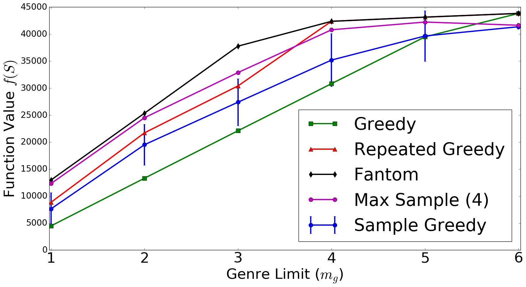
(a) Solution Quality

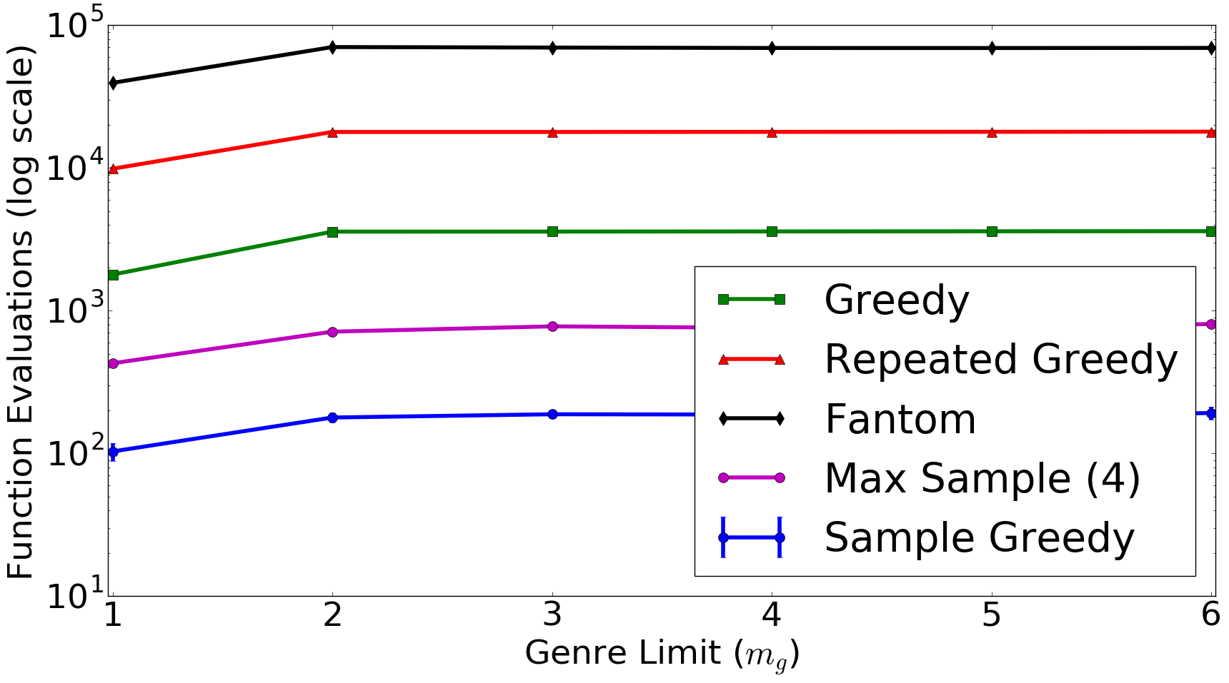
(b) Run Time

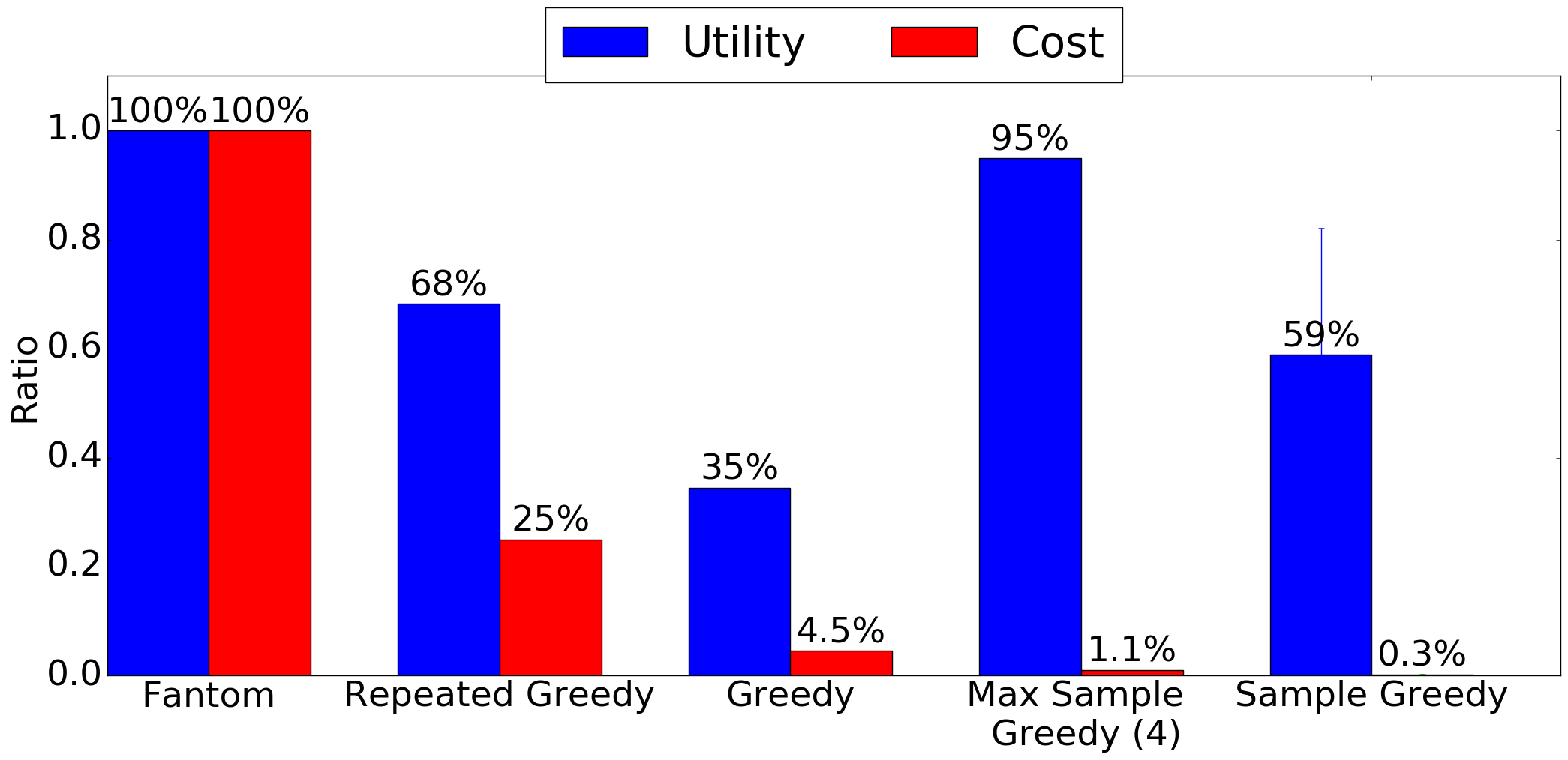
(c) Ratio Comparison $m_{g}=1$

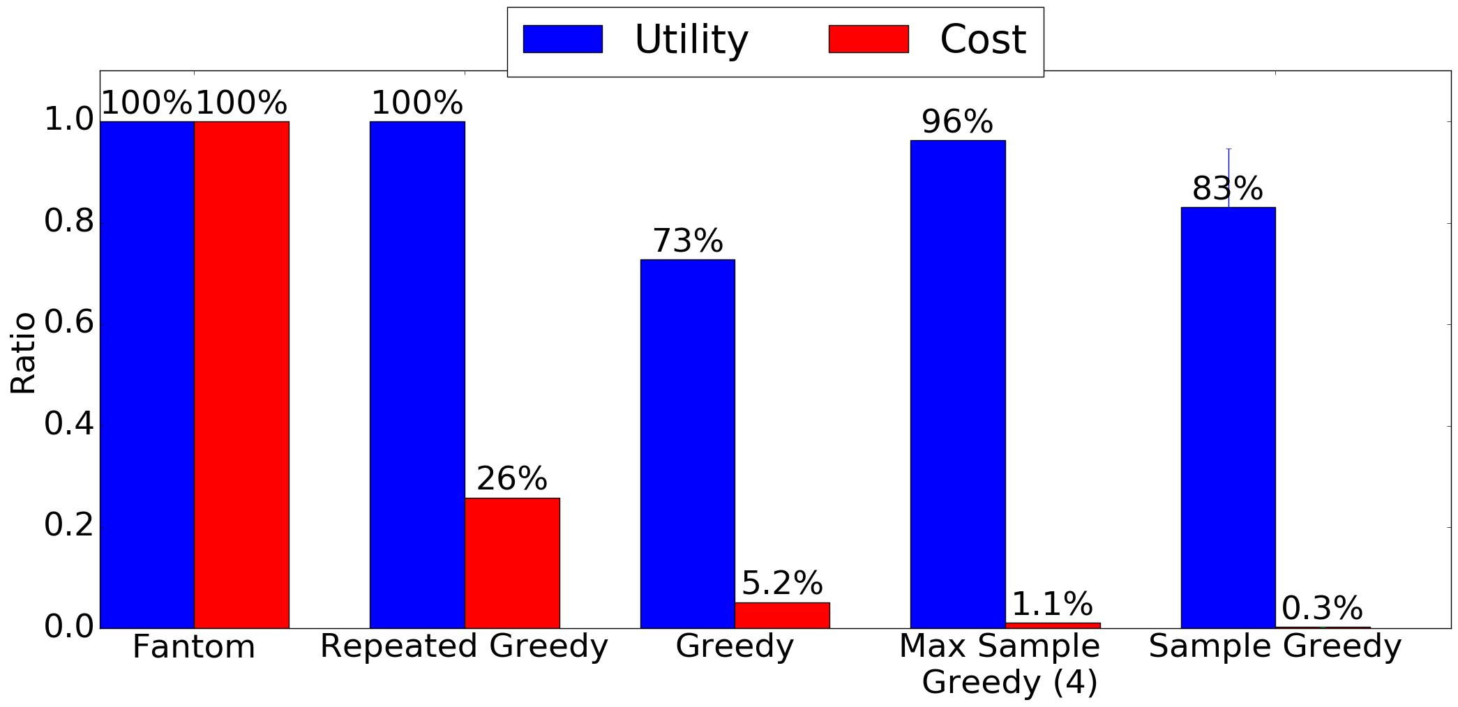
(d) Ratio Comparison $m_{g}=4$

Figure 1: Performance Comparison. 1(a) shows the function value of the returned solutions for tested algorithms with varying genre limit $m_{g}$. 1(b) shows the number of function evaluations on a logarithmic scale with varying genre limit $m_{g}$. 1(c) and 1(d) show the ratio of solution quality and cost with FANTOM as a baseline.

Figure 1(a) shows the value of the solution sets for the various algorithms. As we see from Figure 1(a), FANTOM consistently returns a solution set with the highest function value; however, RepeatedGreedy and SampleGreedy return solution sets with similarly high function values. We see that Max Sample Greedy, even for four runs, significantly increases the performance for more constrained problems. Note that for such more constrained problems, Greedy returns solution sets with much lower function values. Figure 1(b) shows the number of function calls made by each algorithm as the genre limit $m_{g}$ is varied. For each algorithm, the number of function calls remains roughly constant as $m_{g}$ is varied—this is due to the lazy greedy implementation that takes advantage of submodularity to reduce the number of function calls. We see that for our problem instances, RepeatedGreedy runs about an order of magnitude faster than FANTOM and SampleGreedy runs roughly three orders of magnitude faster than FANTOM. Moreover, boosting SampleGreedy by executing it a few times does not incur a significant increase in cost.

To better analyze the tradeoff between the utility of the solution value and the cost of run time, we compare the ratio of these measurements for the various algorithms using FANTOM as a baseline. See Figure 1(c) and 1(d) for these ratio comparisons for genre limits $m_{g}=1$ and $m_{g}=4$, respectively. For the case of $m_{g}=1$, we see that boosted SampleGreedy provides nearly the same utility as FANTOM, while only incurring 1.09% of the computational cost. Likewise, for the case of $m_{g}=4$, RepeatedGreedy achieves the same utility as FANTOM, while incurring only a quarter of the cost. Thus, we may conclude that our algorithms provide solutions whose quality is on par with current state of the art, and yet they run in a small fraction of the time.

Figure 2: Solution Sets. The movies in the solution sets for $m_{g}=1$ returned by FANTOM, Sample Greedy, Repeated Greedy and Greedy are listed here, along with genre information. The favorite genres ($G_{u}$) are in red.

While Greedy may get stuck in poor locally optimal solutions, RepeatedGreedy and SampleGreedy avoid this by greedily combing through the solution space many times and selecting random sets, respectively. Fortunately, the movie recommendation system has a very interpretable solution so we can observe this phenomenon. See Figure 2 for the movies recommended by the different algorithms. Because $m_{g}=1$, we are constrained here to have at most one movie from Adventure, Animation and Fantasy. As seen in Figure 2, FANTOM and SampleGreedy return maximum size solution sets that are both diverse and representative of these genres. On the other hand, Greedy gets stuck choosing a single movie that belongs to all three genres, thus, precluding any other choice of movie from the solution set.

Appendix A Hardness of Maximization over $k$-Extendible Systems

In this appendix, we prove Theorems 3 and 4. The proof consists of two steps. In the first step, we will define two $k$-extendible systems which are indistinguishable in polynomial time. The inapproximability result for linear objectives will follow from the indistinguishability of these systems and the fact that the size of their maximal sets are very different. In the second step we will define monotone submodular objective functions for the two $k$-extendible systems. Using the symmetry gap technique of [Vondrák, 2013], we will show that these objective functions are also indistinguishable, despite being different. Then, we will use the differences between the objective functions to prove the slightly stronger inapproximability result for monotone submodular objectives.

Given three positive integers $k,h$ and $m$ such that $h$ is an integer multiple of $2k$, let us construct a $k$-extendible system ${\cal M}(k,h,m)=({\cal N}_{k.h,m},{\cal I}_{k,h,m})$ as follows. The ground set of the system is ${\cal N}_{k,h,m}=\cup_{i=1}^{h}H_{i}(k,m)$, where $H_{i}(k,m)=\{u_{i,j}~{}|~{}1\leq j\leq km\}$. A set $S\subseteq{\cal N}_{k,h,m}$ is independent (i.e., belongs to ${\cal I}_{k,h,m}$) if and only if it obeys the following inequality:

$$g_{m,k}(|S\cap H_{1}(k,m)|)+|S\setminus H_{1}(k,m)|\leq m\enspace,$$

where the function $g_{m,k}$ is defined by

$$g_{m,k}(x)=\min\left\{x,\frac{2km}{h}\right\}+\max\left\{\frac{x-2km/h}{k},0\right\}\enspace.$$

Intuitively, a set is independent if its elements do not take too many “resources”, where most elements requires a unit of resources, but elements of $H_{1}(k,m)$ take only $1/k$ unit of resources each once there are enough of them. Consequently, the only way to get a large independent set is to pack many $H_{1}(k,m)$ elements.

Lemma 7.

For every choice of $h$ and $m$, ${\cal M}(k,h,m)$ is a $k$-extendible system.

Proof.

First, observe that $g(x)$ is a monotone function, and therefore, a subset of an independent set of ${\cal M}(k,h,m)$ is also independent. Also, $g(0)=0$, and therefore, $\varnothing\in{\cal I}_{k,h,m}$. This proves that ${\cal M}(k,h,m)$ is an independence system. In the rest of the proof we show that it is also $k$-extendible.

Consider an arbitrary independent set $C\in{\cal I}_{k,h,m}$, an independent extension $D$ of $C$ and an element $u\not\in D$ for which $C+u\in{\cal I}_{k,h,m}$. We need to find a subset $Y\subseteq D\setminus C$ of size at most $k$ such that $D\setminus Y+u\in{\cal I}_{k,h,m}$. If $|D\setminus C|\leq k$, then we can simply pick $Y=D\setminus C$. Thus, we can assume from now on that $|D\setminus C|>k$.

Let $\Sigma(S)=g(|S\cap H_{1}(k,m)|)+|S\setminus H_{1}(k,m)|$. By definition, $\Sigma(D)\leq m$ because $D\in{\cal I}_{k,h,m}$. Observe that $g(x)$ has the property that for every $x\geq 0$, $k^{-1}\leq g(x+1)-g(x)\leq 1$. Thus, $\Sigma(S)$ increases by at most $1$ every time that we add an element to $S$, but decreases by at least $1/k$ every time that we remove an element from $S$. Hence, if we let $Y$ be an arbitrary subset of $D\setminus C$ of size $k$, then

$$\Sigma(D\setminus Y+u)\leq\Sigma(D)-\frac{|Y|}{k}+1=\Sigma(D)\leq m\enspace,$$

which implies that $D\setminus Y+u\in{\cal I}_{k,h,m}$. ∎

Before presenting the second $k$-extendible system, let us show that ${\cal M}(k,h,m)$ contains a large independent set.

Observation 2.

${\cal M}(k,h,m)$ contains an independent set whose size is $k(m-2km/h)+2km/h\geq mk(1-2k/h)$. Moreover, there is such set in which all elements belong to $H_{1}(k,m)$.

Proof.

Let $s=k(m-2km/h)+2km/h$, and consider the set $S=\{u_{1,j}\mid 1\leq j\leq s\}$. This is a subset of $H_{1}(k,m)\subseteq{\cal N}_{k,h,m}$ since $s\leq km$. Also,

$$g(|S|)={} g(s)=\min\left\{s,\frac{2km}{h}\right\}+\max\left\{\frac{s-2km/h}{k},0\right\}$$

$$\leq{} \frac{2km}{h}+\max\left\{\frac{[k(m-2km/h)+2km/h]-2km/h}{k},0\right\}$$

$$={} \frac{2km}{h}+\max\left\{m-\frac{2km}{h},0\right\}=m\enspace.$$

Since $S$ contains only elements of $H_{1}(k,m)$, its independence follows from the above inequality. ∎

Let us now define our second $k$-extendible system ${\cal M}^{\prime}(k,h,m)=({\cal N}_{k,h,n},{\cal I}^{\prime}_{k,n})$. The ground set of this system is the same as the ground set of ${\cal M}(k,h,m)$, but a set $S\subseteq{\cal N}_{k,h,m}$ is considered independent in this independence system if and only if its size is at most $m$. Clearly, this is a $k$-extendible system (in fact, it is a uniform matroid). Moreover, note that the ratio between the sizes of the maximal sets in $\cM(k,h,m)$ and $\cM^{\prime}(k,h,m)$ is at least

$$\frac{mk(1-2k/h)}{m}=k(1-2k/h)\enspace.$$

Our plan is to show that it takes exponential time to distinguish between the systems ${\cal M}(k,h,m)$ and ${\cal M}^{\prime}(k,h,m)$, and thus, no polynomial time algorithm can provide an approximation ratio better than this ratio for the problem of maximizing the cardinality function (i.e., the function $f(S)=|S|$) subject to a $k$-extendible system constraint.

Consider a polynomial time deterministic algorithm that gets either ${\cal M}_{k,h,m}$ or ${\cal M}^{\prime}_{k,h,m}$ after a random permutation was applied to the ground set. We will prove that with high probability the algorithm fails to distinguish between the two possible inputs. Notice that by Yao’s lemma, this implies that for every random algorithm there exists a permutation for which the algorithms fails with high probability to distinguish between the inputs.

Assuming our deterministic algorithm gets ${\cal M}^{\prime}_{k,h,m}$, it checks the independence of a polynomial collection of sets. Observe that the sets in this collection do not depend on the permutation because the independence of a set in ${\cal M}^{\prime}_{k,h,m}$ depends only on its size, and thus, the algorithm will take the same execution path given every permutation. If the same algorithm now gets ${\cal M}_{k,h,m}$ instead, it will start checking the independence of the same sets until it will either get a different answer for one of the checks (different than what is expected for ${\cal M}^{\prime}_{k,h,m}$) or it will finish all the checks. Note that in the later case the algorithm must return the same answer that it would have returned had it been given ${\cal M}^{\prime}_{k,h,m}$. Thus, it is enough to upper bound the probability that any given check made by the algorithm will result in a different answer given the inputs ${\cal M}_{k,h,m}$ and ${\cal M}^{\prime}_{k,h,m}$.

Lemma 8.

Following the application of the random ground set permutation, the probability that a set $S$ is independent in ${\cal M}_{k,h,m}$ but not in ${\cal M}^{\prime}_{k,h,m}$, or vice versa, is at most $e^{-\frac{2km}{h^{2}}}$.

Proof.

Observe that as long as we consider a single set, applying the permutation to the ground set is equivalent to replacing $S$ with a random set of the same size. So, we are interested in the independence in ${\cal M}_{k,h,m}$ and ${\cal M}^{\prime}_{k,h,m}$ of a random set of size $|S|$. If $|S|>km$, then the set is never independent in either ${\cal M}_{k,h,m}$ or ${\cal M}^{\prime}_{k,h,m}$, and if $|S|\leq m$, then the set is always independent in both ${\cal M}_{k,h,m}$ and ${\cal M}^{\prime}_{k,h,m}$. Thus, the interesting case is when $m<|S|\leq km$.

Let $X=|S\cap H_{1}(k,m)|$. Notice that $X$ has a hypergeometric distribution, and $\mathbb{E}[X]=|S|/h$. Thus, using bounds given in [Skala, 2013] (these bounds are based on results of [Chvátal, 1979, Hoeffding, 1963]), we get

$$\Pr\left[X\geq\frac{2km}{h}\right]=\Pr\left[X\geq\bE[|X|]+\frac{km}{h}\right]\leq e^{-2\left(\frac{km/h}{|S|}\right)^{2}\cdot|S|}=e^{-\frac{2k^{2}m^{2}}{h^{2}\cdot|S|}}\leq e^{-\frac{2km}{h^{2}}}\enspace.$$

The lemma now follows by observing that $X\leq 2km/h$ implies that $S$ is a dependent set under both ${\cal M}_{k,h,m}$ and ${\cal M}^{\prime}_{k,h,m}$. ∎

We now think of $m$ as going to infinity and of $h$ and $k$ as constants. Notice that given this point of view the size of the ground set $\cN_{k,h,m}$ is $nkh=O(m)$. Thus, the last lemma implies, via the union bound, that with high probability an algorithm making a polynomial number (in the size of the ground set) of independence checks will not be able to distinguishes between the cases in which it gets as input $\cM_{k,h,m}$ or $\cM^{\prime}_{k,h,m}$.

We are now ready to prove Theorem 3.

Proof of Theorem 3.

Consider an algorithm that needs to maximize the cardinality function over the $k$-extendible system $\cM_{k,h,m}$ after the random permutation was applied, and let $T$ be its output set. Notice that $T$ must be independent in $\cM_{k,h,m}$, and thus, its size is always upper bounded by $mk$. Moreover, since the algorithm fails, with high probability, to distinguish between $\cM_{k,h,m}$ and $\cM^{\prime}_{k,h,m}$, $T$ is with high probability also independent in $\cM^{\prime}_{k,h,m}$, and thus, has a size of at most $m$. Therefore, the expected size of $T$ cannot be larger than $m+o(1)$.

On the other hand, Lemma 2 shows that $\cM_{k,h,m}$ contains an independent set of size at least $mk(1-2k/h)$. Thus, the approximation ratio of the algorithm is no better than

$$\frac{mk(1-2k/h)}{m+o(1)}\geq\frac{mk(1-2k/h)}{m}-\frac{k}{m}o(1)=k-2k^{2}/h-o(1)\enspace.$$

Choosing a large enough $h$ (compared to $k$), we can make this approximation ratio larger than $k-\varepsilon$ for any constant $\varepsilon>0$. ∎

To prove a stronger inapproximability result for monotone submodular objectives, we need to associate a monotone submodular function with each one of our $k$-extendible systems. Towards this goal, consider the monotone submodular function $f_{h}:2^{{\cal N}_{h}}\rightarrow\mathbb{R}^{+}$ defined over the ground set ${\cal N}_{h}=[h]$ by

$$f_{h}(S)=\min\{|S|,1\}\enspace.$$

Let $F_{h}\colon[0,1]^{\cN_{h}}\to{\bR_{\geq 0}}$ be the mutlilinear extension of $f_{h}$, i.e., $F_{h}(x)=\bE[f_{h}(R(x))]$ for every vector $x\in[0,1]^{\cN_{h}}$ (where $R(x)$ is a random set containing every element $u\in\cN_{u}$ with probability $x_{u}$, independently). Additionally, given a vector $x\in[0,1]^{{\cal N}_{h}}$, let us define $\bar{x}=(\|x\|_{1}/h)\cdot{\mathbf{1}}_{{\cal N}_{h}}$. Notice that $f_{h}$ is invariant under any permutation of the elements of ${\cal N}_{h}$. Thus, by Lemma 3.2 in [Vondrák, 2013], for every $\varepsilon^{\prime}>0$ there exists $\delta_{h}>0$ and two functions $\hat{F}_{h},\hat{G}_{h}:[0,1]^{{\cal N}_{h}}\rightarrow{\bR_{\geq 0}}$ with the following properties.

• For all $x\in[0,1]^{{\cal N}_{h}}$: $\hat{G}_{h}(x)=\hat{F}_{h}(\bar{x})$.

• For all $x\in[0,1]^{{\cal N}_{h}}$, $|\hat{F}_{h}(x)-F_{h}(x)|\leq\varepsilon^{\prime}$.

• Whenever $|x-\bar{x}|^{2}_{2}\leq\delta_{h}$, $\hat{F}_{h}(x)=\hat{G}_{h}(x)$.

• The first partial derivatives of $\hat{F}_{h}$ and $\hat{G}_{h}$ are absolutely continuous.

• $\frac{\partial\hat{F}_{h}}{\partial x_{u}},\frac{\partial\hat{G}_{h}}{\partial x_{u}}\geq 0$ everywhere for every $u\in{\cal N}_{h}$.

• $\frac{\partial^{2}\hat{F}_{h}}{\partial x_{u}\partial x_{v}},\frac{\partial^{2}\hat{G}_{h}}{\partial x_{u}\partial x_{v}}\leq 0$ almost everywhere for every pair $u,v\in{\cal N}_{h}$.

The objective function we associate with ${\cal M}(k,h,m)$ is $\hat{F}_{h}(y(S))$, where $y(S)$ is a vector in $[0,1]^{{\cal N}_{h}}$ whose $i^{th}$ coordinate is $|S\cap H_{i}(k,m)|/(km)$. Similarly, the objective function we associate with ${\cal M}^{\prime}(k,h,m)$ is $\hat{G}_{h}(y(S))$. Notice that both objective functions are monotone and submodular by Lemma 3.1 of [Vondrák, 2013]. We now bound the maximum value of a set in ${\cal M}(k,h,m)$ and ${\cal M}^{\prime}(k,h,m)$ with respect to their corresponding objective functions.

Lemma 9.

The maximum value of a set in ${\cal M}(k,h,m)$ with respect to the objective $\hat{F}_{h}(y(S))$ is at least $1-2k/h-\varepsilon^{\prime}$.

Proof.

Observation 2 guarantees the existence of an independent set $S\subseteq H_{1}(k,m)$ of size $s\geq k(m-2km/h)$ in ${\cal M}(k,h,m)$. The objective value associated with this set is

$$\hat{F}_{h}(y(S))\geq F_{h}(y(S))-\varepsilon^{\prime}=\frac{s}{km}-\varepsilon^{\prime}\geq\frac{k(m-2km/h)}{km}-\varepsilon^{\prime}\\ =1-2k/h-\varepsilon^{\prime}\enspace.$$

∎

Lemma 10.

The maximum value of a set in ${\cal M}^{\prime}(k,h,m)$ with respect to the objective $\hat{G}_{h}(y(S))$ is at most $1-e^{-1/k}+h^{-1}+\varepsilon^{\prime}$.

Proof.

The objective $\hat{G}_{h}(y(S))$ is monotone. Thus, the maximum value set in ${\cal M}^{\prime}(k,h,m)$ must be of size $m$. Notice that for every set $S$ of this size, we get

$$\hat{G}_{h}(y(S))={} \hat{F}_{h}(\overline{y(S)})=\hat{F}_{h}((kh)^{-1}\cdot{\mathbf{1}}_{{\cal N}_{h}})\leq F_{h}((kh)^{-1}\cdot{\mathbf{1}}_{{\cal N}_{h}})+\varepsilon^{\prime}$$

$$={} 1-\left(1-\frac{1}{kh}\right)^{h}+\varepsilon^{\prime}\leq 1-e^{-1/k}\left(1-\frac{1}{k^{2}h}\right)+\varepsilon^{\prime}\leq 1-e^{-1/k}+h^{-1}+\varepsilon^{\prime}\enspace.$$

∎

As before, our plan is to show that after a random permutation is applied to the ground set it is difficult to distinguish between ${\cal M}(k,h,m)$ and ${\cal M}^{\prime}(k,h,m)$ even when each one of them is accompanied with its associated objective. This will give us an inapproximability result which is roughly equal to the ratio between the bounds given by the last two lemmata.

Observe that Lemma 8 holds regardless of the objective function. Thus, $\cM(k,h,m)$ and $\cM^{\prime}(k,h,m)$ are still polynomially indistinguishable. Additionally, the next lemma shows that their associated objective functions are also polynomially indistinguishable.

Lemma 11.

Following the application of the random ground set permutation, the probability that any given set $S$ gets two different values under the two possible objective functions is at most $2h\cdot e^{-2mk\delta_{h}/h^{2}}$.

Proof.

Recall that, as long as we consider a single set $S$, applying the permutation to the ground set is equivalent to replacing $S$ with a random set of the same size. Hence, we are interested in the value under the two objective functions of a random set of size $|S|$. Define $X_{i}=|S\cap H_{i}(k,m)|$. Since $X_{i}$ has the a hypergeometric distribution, the bound of [Skala, 2013] gives us

$$\Pr\left[X_{i}\geq\frac{|S|}{h}+mk\cdot\sqrt{\frac{\delta_{h}}{h}}\right]={} \Pr\left[X_{i}\geq\mathbb{E}[X_{i}]+mk\cdot\sqrt{\frac{\delta_{h}}{h}}\right]$$

$$\leq{} e^{-2\cdot\left(\frac{mk\cdot\sqrt{\delta_{h}/h}}{|S|}\right)^{2}\cdot|S|}=e^{-\frac{2\delta_{h}}{h}\cdot\frac{m^{2}k^{2}}{|S|}}\leq e^{-2mk\delta_{h}/h^{2}}\enspace.$$

Similarly, we also get

$$\Pr\left[X_{i}\leq\frac{|S|}{h}-mk\cdot\sqrt{\frac{\delta_{h}}{h}}\right]\leq e^{-2mk\delta_{h}/h^{2}}\enspace.$$

Combining both inequalities using the union bound now yields

$$\Pr\left[\left|X_{i}-\frac{|S|}{h}\right|\geq mk\cdot\sqrt{\frac{\delta_{h}}{h}}\right]\leq 2e^{-2mk\delta_{h}/h^{2}}\enspace.$$

Using the union bound again, the probability that $\left|X_{i}-\frac{|S|}{h}\right|\geq mk\cdot\sqrt{\frac{\delta_{h}}{h}}$ for any $1\leq i\leq h$ is at most $2h\cdot e^{-2mk\delta_{h}/h^{2}}$. Thus, to prove the lemma it only remains to show that the value of the two objective functions for $S$ are equal when $\left|X_{i}-\frac{|S|}{h}\right|<mk\cdot\sqrt{\frac{\delta_{h}}{h}}$ for every $1\leq i\leq h$.

Notice that $\overline{y(S)}$ is a vector in which all the coordinates are equal to $|S|/(mkh)$. Thus, the inequality $\left|X_{i}-\frac{|S|}{h}\right|<mk\cdot\sqrt{\frac{\delta_{h}}{h}}$ is equivalent to $[y_{i}(S)-\overline{y_{i}(S)}]<\sqrt{\frac{\delta_{h}}{h}}$. Hence,

$$|y(S)-\overline{y(S)}|_{2}^{2}=\sum_{i=1}^{h}(y_{i}(S)-\overline{y_{i}(S)})^{2}<\sum_{i=1}^{h}\left(\sqrt{\frac{\delta_{h}}{h}}\right)^{2}=\sum_{i=1}^{h}\frac{\delta_{h}}{h}=\delta_{h}\enspace,$$

which implies the lemma by the properties of $\hat{F}_{h}$ and $\hat{G}_{h}$. ∎

Consider a polynomial time deterministic algorithm that gets either ${\cal M}_{k,h,m}$ with its corresponding objective or ${\cal M}^{\prime}_{k,h,m}$ with its corresponding objective after a random permutation was applied to the ground set. Consider first the case that the algorithm gets ${\cal M}^{\prime}_{k,h,m}$ (and its corresponding objective). In this case, the algorithm checks the independence and value of a polynomial collection of sets (we may assume, without loss of generality, that the algorithm checks both things for every set that it checks). As before, one can observe that the sets in this collection do not depend on the permutation because the independence of a set in ${\cal M}^{\prime}_{k,h,m}$ and its value with respect to $\hat{G}_{h}(y(S))=\hat{F}_{h}(\overline{y(S)})$ depend only on the set’s size, which guarantees that the algorithm takes the same execution path given every permutation. If the same algorithm now gets ${\cal M}_{k,h,m}$ instead, it will start checking the independence and values of the same sets until it will either get a different answer for one of the checks (different than what is expected for ${\cal M}^{\prime}_{k,h,m}$) or it will finish all the checks. Note that in the later case the algorithm must return the same answer that it would have returned had it been given ${\cal M}^{\prime}_{k,h,m}$.

By the union bound, Lemmata 8 and 11 imply that the probability that any of the sets whose value or independence is checked by the algorithm will result in a different answer for the two inputs decreases exponentially in $m$, and thus, with high probability the algorithm fails to distinguish between the inputs, and returns the same output for both. Moreover, note that by Yao’s principal this observation extends also to polynomial time randomized algorithms.

We are now ready to prove Theorem 4.

Proof of Theorem 4.

Consider an algorithm that whose objective is to maximize $\hat{F}(y(S))$ over the $k$-extendible system $\cM_{k,h,m}$ after the random permutation was applied, and let $T$ be its output set. Notice that $\hat{F}(y(T))\leq\hat{F}({\mathbf{1}}_{\cN_{h}})\leq F({\mathbf{1}}_{\cN_{h}})+\varepsilon^{\prime}=1+\varepsilon^{\prime}$. Moreover, the algorithm fails, with high probability, to distinguish between $\cM_{k,h,m}$ and $\cM^{\prime}_{k,h,m}$. Thus, with high probability $T$ is independent in $\cM^{\prime}(k,h,m)$ and has the same value under both objective functions $\hat{F}(y(S))$ and $\hat{G}(y(S))$, which implies, by Lemma 10, $\hat{F}(y(S))=\hat{G}(y(S))\leq 1-e^{-1/k}+h^{-1}+\varepsilon^{\prime}$. Hence, in conclusion we proved

$$\bE[\hat{F}(y(T))]\leq 1-e^{-1/k}+h^{-1}+\varepsilon^{\prime}+o(1)\enspace.$$

On the other hand, Lemma 9 shows that $\cM_{k,h,m}$ contains an independent set of value of at least $1-2k/h-\varepsilon^{\prime}$ (with respect to $\hat{F}(y(S))$). Thus, the approximation ratio of the algorithm is no better than

$$\frac{1-2k/h-\varepsilon^{\prime}}{1-e^{-1/k}+h^{-1}+\varepsilon^{\prime}+o(1)}$$

$$\geq{} (1-e^{-1/k}+h^{-1}+\varepsilon^{\prime}+o(1))^{-1}-(1-e^{-1/k})^{-1}(2k/h+\varepsilon^{\prime})$$

$$\geq{} (1-e^{-1/k})^{-1}-(1-e^{-1/k})^{-2}(h^{-1}+\varepsilon^{\prime}+o(1))-(1-e^{-1/k})^{-1}(2k/h+\varepsilon^{\prime})$$

$$\geq{} (1-e^{-1/k})^{-1}-(k+1)^{2}(h^{-1}+\varepsilon^{\prime}+o(1))-(k+1)(2k/h+\varepsilon^{\prime})\enspace,$$

where the last inequality holds since $1-e^{-1/k}\geq(k+1)^{-1}$. Choosing a large enough $h$ (compared to $k$) and a small enough $\varepsilon^{\prime}$ (again, compared to $k$), we can make this approximation ratio larger than $(1-e^{-1/k})^{-1}-\varepsilon$ for any constant $\varepsilon>0$. ∎

Appendix B Improved Approximation Guarantee for Linear Functions

In Section 5 we described Algorithm 2, which obtains a $(k+1)$-approximation for the maximization of a monotone submodular function subject to a $k$-extendible system constraint. One can observe that the approximation ratio of this algorithm is no better than $k+1$ even when the function is linear since it takes no element with probability larger than $(k+1)^{-1}$. In this appendix we show that if the algorithm is allowed to select each element with probability $k^{-1}$, then its approximation ratio for linear functions improves to $k$; which proves the guarantee of Theorem 1 for linear objectives.

Specifically, we consider in this appendix a variant of Algorithm 2 in which the sampling probability in Line 2 is changed to $k^{-1}$. Similarly, the probability in Line 3 of Algorithm 3 is also changed to $k^{-1}$ in order to keep the two algorithms equivalent. In the rest of this appendix, any reference to Algorithms 2 and 3 should be implicitly understood as a reference to the variants of these algorithms with the above changes.

The analysis we present here for Algorithm 3 (and thus, also for its equivalent Algorithm 2) is very similar to the one given in Section 5, and it is based on the same ideas. However, slightly more care is necessary in order to establish the improved approximation ratio of $k$. We begin with the following lemma, which corresponds to Lemma 4 from Section 5. For every $u\in\cN$, let $Y_{u}$ be a random variable which takes the value $1$ if $u\in S$ and, in addition, $u$ does not belong to $O$ at the beginning of the iteration in which $u$ is considered. In every other case the value of $Y_{u}$ is $0$.

Lemma 12.

$f(S)\geq f(\text{OPT})-\sum\limits_{u\in\mathcal{N}}[|O_{u}|-Y_{u}]f(u)$.

Proof.

The proof of Lemma 4 begins by showing that $f(S)\geq f(O)$. This part of the proof is still true since it is independent of the sampling probability. Thus, we only need to show that

$$f(O)\geq f(\text{OPT})-\sum\limits_{u\in\mathcal{N}}[|O_{u}|-Y_{u}]f(u)\enspace.$$

Recall that $O$ beings as equal to OPT. Thus, to prove the last inequality it is enough to show that the second term on its right hand side is an upper bound on the decrease in the value of $O$ over time. In the rest of the proof we do this by showing that $[|O_{u}|-Y_{u}]f(u)$ is an upper bound on the decrease in the value of $O$ in the iteration in which $u$ is considered, and is equal to $0$ when $u$ is not considered at all.

Let us first consider the case that $u$ is not considered at all. In this case, by definition, $O_{u}=\varnothing$ and $Y_{u}=0$, which imply together $[|O_{u}|-Y_{u}]f(u)=0\cdot f(u)=0$. Consider now the case that $u$ is considered by Algorithm 3. In this case $O$ is changed during the iteration in which $u$ is considered in two ways. First, the elements of $O_{u}$ are removed from $O$, and second, $u$ is added to $O$ if it is added to $S$ and it does not already belong to $O$. Thus, the decrease in the value of $O$ during this iteration can be written as

$$\sum_{v\in O_{u}}f(v)-Y_{u}\cdot f(u)\enspace.$$

To see why this expression is lower bounded by $[|O_{u}|-Y_{u}]f(u)$, we recall that in the proof of Lemma 4 we showed that $f(v|S_{u})\leq f(u|S_{u})$ for every $v\in O_{u}$, which implies, since $f$ is linear, $f(v)\leq f(u)$ for every such element $v$. ∎

The next lemma corresponds to Lemma 5 from Section 5. We omit its proof since it is completely identical to the proof of Lemma 5 up to change in the sampling probability.

Lemma 13.

$\mathbb{E}[f(S)]\geq\frac{1}{k}\sum\limits_{u\in\mathcal{N}}\mathbb{E}[X_{u}\Delta f(u|S_{u})]=\frac{1}{k}\sum\limits_{u\in\mathcal{N}}\mathbb{E}[X_{u}]f(u)$.

We need one last lemma which corresponds to Lemma 6 from Section 5. The role of this lemma is to relate terms appearing in the last two lemmata.

Lemma 14.

For every element $u\in\mathcal{N}$,

$$\mathbb{E}[|O_{u}|-Y_{u}]\leq\frac{k-1}{k}\mathbb{E}[X_{u}]\enspace.$$ (9)

Proof.

As in the proofs of Lemma 6, let $\mathcal{E}_{u}$ be an arbitrary event specifying all random decisions made by Algorithm 3 up until the iteration in which it considers $u$ if $u$ is considered, or all random decisions made by Algorithm 3 throughout its execution if it never considers $u$. By the law of total probability, since these events are disjoint, it is enough to prove Inequality (9) conditioned on every such event $\mathcal{E}_{u}$. If $\mathcal{E}_{u}$ implies that $u$ is not considered, then $|O_{u}|$, $X_{u}$ and $Y_{u}$ are all $0$ conditioned on $\mathcal{E}_{u}$, and thus, the inequality holds as an equality. Thus, we may assume in the rest of the proof that $\mathcal{E}_{u}$ implies that $u$ is considered by Algorithm 3. Notice that, conditioned on $\cE_{u}$, $X_{u}$ takes the value $1$. Hence, Inequality (9) reduces to

$$\mathbb{E}[|O_{u}|-Y_{u}\mid\mathcal{E}_{u}]\leq\frac{k-1}{k}\enspace.$$

There are now two cases to consider. The first case is that $\mathcal{E}_{u}$ implies that $u\in O$ at the beginning of the iteration in which Algorithm 3 considers $u$. In this case $Y_{u}=0$, and in addition, $O_{u}$ is empty if $u$ is added to $S$, and is $\{u\}$ if $u$ is not added to $S$. As $u$ is added to $S$ with probability $\frac{1}{k}$, this gives

$$\mathbb{E}[|O_{u}|-Y_{u}\mid\mathcal{E}_{u}]\leq\frac{1}{k}\cdot|\varnothing|+\left(1-\frac{1}{k}\right)|\{u\}|=\frac{k-1}{k}\enspace,$$

and we are done. Consider now the case that $\mathcal{E}_{u}$ implies that $u\not\in O$ at the beginning of the iteration in which Algorithm 3 considers $u$. In this case, if $u$ is not added to $S$, then we get $Y_{u}=0$ and $O_{u}=\varnothing$. In contrast, if $u$ is added to $S$, then $Y_{u}=1$ by definition and $|O_{u}|\leq k$ by the discussion following Algorithm 3. As $u$ is, again, added to $S$ with probability $\frac{1}{k}$, we get in this case

$$\mathbb{E}[|O_{u}|-Y_{u}|\mid\mathcal{E}_{u}]\leq\frac{1}{k}\cdot(k-1)+\left(1-\frac{1}{k}\right)|\varnothing|=\frac{k-1}{k}\enspace.\qed$$

We are now ready to prove the guarantee of Theorem 1 for linear objectives.

Proof of Theorem 1 for linear objectives..

We prove here that the approximation ratio guaranteed by Theorem 1 for linear objectives is obtained by (the modified) Algorithm 2. As discussed earlier, Algorithms 2 and 3 have identical output distributions, and so it suffices to show that Algorithm 3 achieves this approximation ratio. Note that

$$\mathbb{E}[f(S)] \geq f(\text{OPT})-\sum\limits_{u\in\mathcal{N}}\bE[|O_{u}|-Y_{u}]f(u)$$ (Lemma 12)

$$\geq f(\text{OPT})-\frac{k-1}{k}\sum\limits_{u\in\mathcal{N}}\bE[X_{u}]f(u)$$ (Lemma 14)

$$\geq f(\text{OPT})-(k-1)\mathbb{E}[f(S)]\enspace.$$ (Lemma 13)

The proof now completes by rearranging the above inequality. ∎

References

- Badanidiyuru and Vondrák [2014] Ashwinkumar Badanidiyuru and Jan Vondrák. Fast algorithms for maximizing submodular functions. In SODA, 2014.
- Buchbinder and Feldman [2016a] Niv Buchbinder and Moran Feldman. Constrained submodular maximization via a non-symmetric technique. CoRR, abs/1611.03253, 2016a.
- Buchbinder and Feldman [2016b] Niv Buchbinder and Moran Feldman. Deterministic algorithms for submodular maximization problems. In SODA, 2016b.
- Buchbinder et al. [2014] Niv Buchbinder, Moran Feldman, Joesph (Seffi) Naor, and Roy Schwartz. Submodular maximization with cardinality constrains. In SODA, 2014.
- Buchbinder et al. [2015a] Niv Buchbinder, Moran Feldman, Joseph Naor, and Roy Schwartz. A tight linear time (1/2)-approximation for unconstrained submodular maximization. SIAM J. Comput., 44(5):1384–1402, 2015a.
- Buchbinder et al. [2015b] Niv Buchbinder, Moran Feldman, and Roy Schwartz. Comparing apples and oranges: Query tradeoff in submodular maximization. In SODA, 2015b.
- Călinescu et al. [2011] Gruia Călinescu, Chandra Chekuri, Martin Pál, and Jan Vondrák. Maximizing a monotone submodular function subject to a matroid constraint. SIAM Journal on Computing, 2011.
- Candés and Recht [2008] Emmanuel J. Candés and Benjamin Recht. Exact matrix completion via convex optimization. In Foundations of Computational Mathematics, 2008.
- Chvátal [1979] Vašek Chvátal. The tail of the hypergeometric distribution. Discrete Mathematics, 25(3):285–287, 1979.
- Edmonds [1971] Jack Edmonds. Matroids and the greedy algorithm. Mathematical programming, 1971.
- El-Arini et al. [2009] Khalid El-Arini, Gaurav Veda, Dafna Shahaf, and Carlos Guestrin. Turning down the noise in the blogosphere. In KDD, 2009.
- Ene and Nguyen [2016] Alina Ene and Huy L. Nguyen. Constrained submodular maximization: Beyond 1/e. In FOCS, 2016.
- Feige et al. [2011] Uriel Feige, Vahab S. Mirrokni, and Jan Vondrák. Maximizing non-monotone submodular functions. SIAM Journal on Computing, 2011.
- Feldman et al. [2011a] Moran Feldman, Joseph Naor, and Roy Schwartz. A unified continuous greedy algorithm for submodular maximization. In FOCS, 2011a.
- Feldman et al. [2011b] Moran Feldman, Joseph Naor, Roy Schwartz, and Justin Ward. Improved approximations for k-exchange systems - (extended abstract). In ESA, 2011b.
- Fisher et al. [1978] Marshall L. Fisher, George L. Nemhauser, and Laurence A. Wolsey. An analysis of approximations for maximizing submodular set functions—II. Mathematical Programming, 8:73–87, 1978.
- Fujishige [2005] Satoru Fujishige. Submodular functions and optimization. Elsevier Science, 2nd edition, 2005.
- Gharan and Vondrák [2011] Shayan Oveis Gharan and Jan Vondrák. Submodular maximization by simulated annealing. In SODA, 2011.
- Gillenwater et al. [2012] Jennifer Gillenwater, Alex Kulesza, and Ben Taskar. Near-optimal MAP inference for determinantal point processes. In NIPS, 2012.
- Gomez Rodriguez et al. [2010] Manuel Gomez Rodriguez, Jure Leskovec, and Andreas Krause. Inferring networks of diffusion and influence. In KDD, 2010.
- Guestrin et al. [2005] Carlos Guestrin, Andreas Krause, and Ajit Paul Singh. Near-optimal sensor placements in gaussian processes. In ICML, 2005.
- Gupta et al. [2010] Anupam Gupta, Aaron Roth, Grant Schoenebeck, and Kunal Talwar. Constrained non-monotone submodular maximization: Offline and secretary algorithms. In WINE, 2010.
- Hastie et al. [2015] Trevor Hastie, Rahul Mazumder, Jason D. Lee, and Rexa Zadeh. Matrix completion and low-rank svd via fast alternating least squares. In Journal of Machine Learning Research, 2015.
- Hoeffding [1963] Wassily Hoeffding. Probability inequalities for sums of bounded random variables. Journal of the American Statistical Association, 1963.
- Jenkyns [1976] Tom A. Jenkyns. The efficacy of the “greedy” algorithm. In South Eastern Conference on Combinatorics, Graph Theory and Computing, 1976.
- Kempe et al. [2003] David Kempe, Jon Kleinberg, and Éva Tardos. Maximizing the spread of influence through a social network. In KDD, 2003.
- Kirchhoff and Bilmes [2014] Katrin Kirchhoff and Jeff Bilmes. Submodularity for data selection in statistical machine translation. In EMNLP, 2014.
- Lee et al. [2010] Jon Lee, Maxim Sviridenko, and Jan Vondrák. Submodular maximization over multiple matroids via generalized exchange properties. Mathematics of Operations Research, 2010.
- Leskovec et al. [2007] Jure Leskovec, Andreas Krause, Carlos Guestrin, Christos Faloutsos, Jeanne Van Briesen, and Natalie Glance. Cost-effective outbreak detection in networks. In KDD, 2007.
- Lin and Bilmes [2011] Hui Lin and Jeff Bilmes. A class of submodular functions for document summarization. In ACL, 2011.
- Lindgren et al. [2015] Erik M. Lindgren, Shanshan Wu, and Alexandros G. Dimakis. Sparse and greedy: Sparsifying submodular facility location problems. In NIPS Workshop on Optimization for Machine Learning, 2015.
- Mestre [2006] Julián Mestre. Greedy in approximation algorithms. In ESA, pages 528–539, 2006.