Biphoton Interference in a Double-Slit Experiment

Adouble-slit experiment with entangled photons is theoretically analyzed. It is shown that, under suitable conditions, two entangled photons of wavelength $\lambda$ can behave like a biphoton of wavelength $\lambda/2$. The interference of these biphotons, passing through a double-slit can be obtained by detecting both photons of the pair at the same position. This is in agreement with the results of an earlier experiment. More interestingly, we show that even if the two entangled photons are separated by a polarizing beam splitter, they can still behave like a biphoton of wavelength $\lambda/2$. In this modified setup, the two separated photons passing through two different double-slits, surprisingly show an interference corresponding to a wavelength $\lambda/2$, instead of $\lambda$ which is the wavelength of each photon. We point out two experiments that have been carried out in different contexts, which saw the effect predicted here without realizing this connection.
Quanta 2018; 7: 1–6.

1 Introduction

Quantum mechanics has taught us that wave nature and particle nature are two complementary aspects of the same entity [1]. Whether we talk of massive particles or quanta of light, both can behave like particles and waves in different situations. Young’s double-slit experiment carried out with individual particles showed that a particle passes through two slits and interferes with itself [2]. Later it was demonstrated that much larger particles such as $C_{60}$ molecules can also show interference [3]. It has been convincingly argued that instead of calling them waves or particles, such entities should be called quantons [4, p. 235][5]. Going beyond this, quantum mechanics also tells us that a group of entities, e.g., many photons together, can behave as a single quanton. Consequences of this on interference experiments with many particles, has only been recognized relatively recently [6].

First, we briefly explain the idea which motivated Jacobson and collaborators [6] to propose that many photons can behave as a single quanton in an interference experiment. Consider a beam of diatomic iodine molecules $I_{2}$ each with mass $2m$, traveling with a velocity $v$, passing through a double-slit. The resulting interference would be in accordance with a de Broglie wavelength $\lambda_{2m}=h/2mv$. But suppose that the molecule dissociates on the way, and only separate iodine atoms, each of mass $m$, pass through the double-slit. Then the resulting interference would be in accordance with a de Broglie wavelength $\lambda_{m}=h/mv$, which shows that $\lambda_{2m}=\lambda_{m}/2$. More generally, $N$ particles with a de Broglie wavelength $\lambda$, can behave as single quanton of wavelength $\lambda/N$. The same should hold for photons too. An experiment was subsequently carried out which measured the de Broglie wavelength of a two-photon wavepacket [7].

 
This is an open access article distributed under the terms of the Creative Commons Attribution License CC-BY-3.0, which permits unrestricted use, distribution, and reproduction in any medium, provided the original author and source are credited.

In the following we carry out a wave-packet analysis of two entangled photons, typically generated in a type-I spontaneous parametric down conversion (SPDC) process, and analyze the situation in which they can behave like a single quanton.

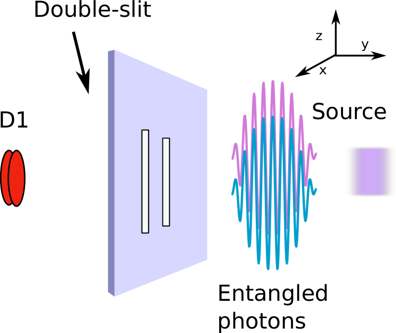
Figure 1: Schematic diagram for Young’s double-slit experiment with entangled photons. Detector D1 is capable of detecting pairs of photons. It should be able to discriminate between one-photon and two-photons events.

2 Theoretical analysis

2.1 Entangled photons

A well known state to describe momentum-entangled particles was discussed by Einstein, Podolsky and Rosen (EPR) [8]

$$\Psi_{\textrm{EPR}}(x_{1},x_{2})=A\!\int_{-\infty}^{\infty}e^{-{\imath px_{2}\over\hbar}}e^{\frac{\imath px_{1}}{\hbar}}dp.$$ (1)

This so-called EPR state does capture the properties of entangled particles well, but has some disadvantages like not being normalized, and also not describing varying degree of entanglement. The best state to describe momentum-entangled particles is the generalized EPR state [9, 10]

$$\Psi(x_{1},x_{2})=A\!\int_{-\infty}^{\infty}e^{-{p^{2}\sigma^{2}\over\hbar^{2}}}e^{-{\imath px_{2}\over\hbar}}e^{\frac{\imath px_{1}}{\hbar}}e^{-{(x_{1}+x_{2})^{2}\over 4\Omega^{2}}}dp,$$ (2)

where $A$ is a normalization constant, and $\sigma,\Omega$ are certain parameters. In the limit $\sigma\to 0,\leavevmode\nobreak\ \leavevmode\nobreak\ \Omega\to\infty$ the state (2) reduces to the EPR state (1).

After performing the integration over $p$, (2) reduces to

$$\Psi(x_{1},x_{2})={1\over\sqrt{\pi\sigma\Omega}}e^{\frac{-(x_{1}-x_{2})^{2}}{4\sigma^{2}}}e^{\frac{-(x_{1}+x_{2})^{2}}{4\Omega^{2}}}.$$ (3)

It is straightforward to show that $\Omega$ and $\hbar/\sigma$ quantify the position and momentum spread of the particles in the $x$-direction because the uncertainty in position and the wave-vector of the two photons, along the $z$-axis, is given by

$$\Delta x_{1}=\Delta x_{2}=\sqrt{\Omega^{2}+\sigma^{2}},\Delta k_{1x}=\Delta k_{2x}=\tfrac{1}{4}\sqrt{{1\over\sigma^{2}}+{1\over\Omega^{2}}}\leavevmode\nobreak\ .$$ (4)

Notice that for $\sigma=\Omega$, the state is no longer entangled, and factors into a product of two Gaussians centered at $x_{1}=0$ and $x_{2}=0$, respectively. The state (3) also describes well the two-photon mode function at the output of the type-I crystal in SPDC generation [11, 12].

The experiment is schematically described in Figure 1. Entangled particles (generally photons) emerge from a source, and pass through a double-slit to reach a screen or a detector D1 which is movable along the $x$-axis. We assume that at time $t=0$, the two particles are in the state (3), and travel along the $y$-axis, towards a double-slit, with average momenta $p_{0}$. Each particle can then be described as a quanton with a wavelength $\lambda=h/p_{0}$. For photons, the wavelength is fixed as $\lambda=2\pi/k_{0}$.

2.2 Time evolution

Time evolution of a one-dimensional wave-packet, along $x$-axis, is given by

$$\psi(x,t)={1\over\sqrt{2\pi}}\int_{-\infty}^{\infty}\tilde{\psi}(k_{x})\exp\left[\imath(k_{x}x-\omega(k_{x})t)\right]dk_{x}.$$ (5)

For massive particles, one would have assumed $\omega(k_{x})=\hbar k_{x}^{2}/2m$. For photons one can work within the Fresnel approximation, ($k_{y}\approx k_{0}$, $k_{x}\ll k_{y}$) to write $\omega(k_{x})$ as [13]

$$\omega(k_{x})=c\sqrt{k_{x}^{2}+k_{y}^{2}}\approx ck_{0}+{ck_{x}^{2}\over 2k_{0}}.$$ (6)

So the spread of a photon wave-packet in the $x$-direction, which is moving essentially along $y$-direction, is given by

$$\psi(x,t)={e^{-\imath k_{0}t}\over\sqrt{2\pi}}\int_{-\infty}^{\infty}\tilde{\psi}(k_{x})e^{\imath k_{x}x}e^{-\imath ctk_{x}^{2}/2k_{0}}dk_{x}\leavevmode\nobreak\ .$$ (7)

Using the above, the time propagation kernel for the two photons can be written as

$$K_{1}(x_{1},x_{1}^{\prime},t) = \sqrt{1\over\imath\lambda ct}\exp\left[{-\pi(x_{1}-x_{1}^{\prime})^{2}\over\imath\lambda ct}\right],$$

$$K_{2}(x_{2},x_{2}^{\prime},t) = \sqrt{1\over\imath\lambda ct}\exp\left[{-\pi(x_{2}-x_{2}^{\prime})^{2}\over\imath\lambda ct}\right],$$ (8)

and the two-particle state after a time $t$ is given by

$$\Psi(x_{1},x_{2},t) = \int_{-\infty}^{\infty}\int_{-\infty}^{\infty}K_{1}(x_{1},x_{1}^{\prime},t)\times$$

$$\qquad K_{2}(x_{2},x_{2}^{\prime},t)\Psi(x_{1}^{\prime},x_{2}^{\prime})\leavevmode\nobreak\ dx_{1}^{\prime}dx_{2}^{\prime}.$$

At this stage it is convenient to introduce new coordinates for the entangled particles: $r=(x_{1}+x_{2})/2,\leavevmode\nobreak\ \leavevmode\nobreak\ q=(x_{1}-x_{2})/2$. The state of the entangled particles, at time $t=0$, can then be written as

$$\Psi(r,q)={1\over\sqrt{\pi\sigma\Omega}}e^{-q^{2}/\sigma^{2}}e^{-r^{2}/\Omega^{2}}.$$ (10)

The time-propagator, in the new coordinates, can be written as

$$K_{r}(r,r^{\prime},t) = \sqrt{1\over\imath\lambda ct}\exp\left[{-2\pi(r-r^{\prime})^{2}\over\imath\lambda ct}\right]$$

$$K_{q}(q,q^{\prime},t) = \sqrt{1\over\imath\lambda ct}\exp\left[{-2\pi(q-q^{\prime})^{2}\over\imath\lambda ct}\right].$$ (11)

The state after a general time $t$ can then be evaluated as

$$\Psi(r,q,t) = \int_{-\infty}^{\infty}\int_{-\infty}^{\infty}K_{r}(r,r^{\prime},t)\times$$ (12)

$$\qquad K_{q}(q,q^{\prime},t)\Psi(r^{\prime},q^{\prime})\leavevmode\nobreak\ dr^{\prime}dq^{\prime}.$$

Let us assume that during a time $t_{0}$, the photons travel a distance $L$, from the source to the double-slit, and the state at the double-slit takes the form:

$$\Psi(r,q,t_{0})=C\exp\left({-q^{2}\over\sigma^{2}+\imath\alpha}\right)\exp\left({-r^{2}\over\Omega^{2}+\imath\alpha}\right),$$ (13)

where $C=\frac{1}{\sqrt{\pi\sqrt{\sigma+\imath{\alpha/\sigma}}\sqrt{\Omega+\imath{\alpha/\Omega}}}}$, and $\alpha=\lambda L/2\pi$.

2.3 Effect of the double-slit

After a time $t_{0}$, the two photons reach the double-slit and pass through it to emerge on the other side. A rigorous, but immensely difficult approach would be to consider the double-slit as a potential, and let the two photons evolve under the action of that potential. We take a simpler and less rigorous approach, by assuming that the effect of the double-slit is to truncate the wave-function abruptly such that only the part of the wave function in the region $-{d\over 2}-{\epsilon\over 2}\leq x_{1},x_{2}\leq-{d\over 2}+{\epsilon\over 2}$ and ${d\over 2}-{\epsilon\over 2}\leq x_{1},x_{2}\leq{d\over 2}+{\epsilon\over 2}$ survives. This region corresponds to the region of the two slits, if the slits of width $\epsilon$ are located at $x=-{d\over 2}$ and $x={d\over 2}$. In our new coordinates, this region corresponds approximately to (a) $\pm{d\over 2}-{\epsilon\over 2}\leq r\leq\pm{d\over 2}+{\epsilon\over 2}$ together with $-{\epsilon\over 2}\leq q\leq{\epsilon\over 2}$ and (b) $\pm{d\over 2}-{\epsilon\over 2}\leq q\leq\pm{d\over 2}+{\epsilon\over 2}$ together with $-{\epsilon\over 2}\leq r\leq{\epsilon\over 2}$. This is not completely accurate as far as $\epsilon$ is concerned, but since the interference will be seen in the limit of very small $\epsilon$, this approximation suffices for our purpose. Case (a) corresponds to both photons passing through the same slit, whereas case (b) corresponds to both photons passing through different slits. Notice that if the two photons have a high spatial correlation, case (b) is expected to have very low probability.

The two photons travel a distance $D=ct$ to reach the screen/detector. The state at the screen is given by the following time-evolution

$$\Psi(r,q,t) = \int_{-{d\over 2}-{\epsilon\over 2}}^{-{d\over 2}+{\epsilon\over 2}}dr^{\prime}K_{r}(t)\int_{-{\epsilon\over 2}}^{{\epsilon\over 2}}dq^{\prime}K_{q}(t)\Psi(r^{\prime},q^{\prime},t_{0})$$

$$+ \int_{{d\over 2}-{\epsilon\over 2}}^{{d\over 2}+{\epsilon\over 2}}dr^{\prime}K_{r}(t)\int_{-{\epsilon\over 2}}^{{\epsilon\over 2}}dq^{\prime}K_{q}(t)\Psi(r^{\prime},q^{\prime},t_{0})$$

$$+ \int_{-{d\over 2}-{\epsilon\over 2}}^{-{d\over 2}+{\epsilon\over 2}}dq^{\prime}K_{q}(t)\int_{-{\epsilon\over 2}}^{{\epsilon\over 2}}dr^{\prime}K_{r}(t)\Psi(r^{\prime},q^{\prime},t_{0})$$

$$+ \int_{{d\over 2}-{\epsilon\over 2}}^{{d\over 2}+{\epsilon\over 2}}dq^{\prime}K_{q}(t)\int_{-{\epsilon\over 2}}^{{\epsilon\over 2}}dr^{\prime}K_{r}(t)\Psi(r^{\prime},q^{\prime},t_{0}),$$

where the propagator and the initial state are given by (11) and (13), respectively. For brevity, the $q,q^{\prime},r,r^{\prime}$ dependence of the propagators has been suppressed. A typical integral in (LABEL:psiformal) looks like the following:

$$I = \int_{{d\over 2}-{\epsilon\over 2}}^{{d\over 2}+{\epsilon\over 2}}\exp\left[{-{2\pi(r-r^{\prime})^{2}\over\imath\lambda L}}\right]\exp\left[{-{r^{\prime 2}\over\Omega^{2}+\imath\alpha}}\right]dr^{\prime}.$$

Since the profile of the incoming beam is wide, $\Omega^{2}\gg\lambda L/2\pi$. The slit width $\epsilon$ is assumed to be very small. Since in the integral above, $r^{\prime}$ varies only between ${d\over 2}-{\epsilon\over 2}$ to ${d\over 2}+{\epsilon\over 2}$, the term $\exp\left({-{r^{\prime 2}\over\Omega^{2}+\imath\alpha}}\right)$ can be assumed to be constant in this region, and equal to $\exp\left({-{d^{2}/4\over\Omega^{2}+\imath\alpha}}\right)$. Keeping in mind the smallness of $\epsilon$, we can make an additional approximation, $(r-r^{\prime})^{2}\approx(r-{d\over 2})^{2}-2(r-{d\over 2})(r^{\prime}-{d\over 2})$, ignoring terms of order $\epsilon^{2}$. With these assumptions, the integral in (LABEL:term) can be approximated by

$$I \approx e^{2\pi\imath(r-d/2)^{2}\over\lambda D}e^{-{d^{2}/4\over\Omega^{2}+\imath\alpha}}\int_{{d\over 2}-{\epsilon\over 2}}^{{d\over 2}+{\epsilon\over 2}}e^{-{4\pi\imath(r-d/2)(r^{\prime}-d/2)\over\lambda D}}dr^{\prime}$$ (16)

$$= e^{2\pi\imath(r-d/2)^{2}\over\lambda D}e^{-{d^{2}/4\over\Omega^{2}+\imath\alpha}}\tfrac{\sin\left(2\pi(r-d/2)\epsilon/\lambda D\right)}{2\pi(r-d/2)/\lambda D}.$$

If similar algebra is carried out over all the integrals in (LABEL:psiformal), one obtains the following form of the final state of the biphoton

$$\Psi(r,q,t) = C_{t}\left(e^{{2\pi\imath\over\lambda D}(r-{d\over 2})^{2}}e^{{2\pi\imath\over\lambda D}q^{2}}f(r-\tfrac{d}{2})f(q)e^{-{d^{2}\Omega^{2}\over 4\Omega^{4}+4\alpha^{2}}}\right.$$

$$\left.+e^{{2\pi\imath\over\lambda D}(r+\tfrac{d}{2})^{2}}e^{{2\pi\imath\over\lambda D}q^{2}}f(r+\tfrac{d}{2})f(q)e^{-{d^{2}\Omega^{2}\over 4\Omega^{4}+4\alpha^{2}}}\right.$$

$$\left.+e^{{2\pi\imath\over\lambda D}(q+\tfrac{d}{2})^{2}}e^{{2\pi\imath\over\lambda D}r^{2}}f(q+\tfrac{d}{2})f(r)e^{-{d^{2}\sigma^{2}\over 4\sigma^{4}+4\alpha^{2}}}\right.$$

$$\left.+e^{{2\pi\imath\over\lambda D}(q-\tfrac{d}{2})^{2}}e^{{2\pi\imath\over\lambda D}r^{2}}f(q-\tfrac{d}{2})f(r)e^{-{d^{2}\sigma^{2}\over 4\sigma^{4}+4\alpha^{2}}}\right),$$

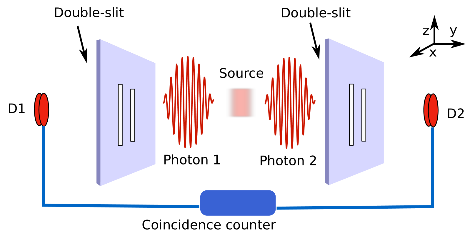
Figure 2: Schematic diagram for the proposed nonlocal biphoton experiment. Photons 1 and 2 effectively move in opposite directions along $y$-axis. Detectors D1 and D2 move along the $x$-axis in synchrony such that their $x$-positions are always the same. They also count the photons in coincidence.

where $C_{t}={\imath\over\lambda D}(\pi)^{-1/2}(\sigma+\imath{\imath\alpha\over\sigma})^{-1/4}(\Omega+\imath{\imath\alpha\over\Omega})^{-1/4}$, and $f(x)\equiv\frac{\sin\left({2\pi x\epsilon/\lambda D}\right)}{2\pi x/\lambda D}$ governs the spatial spread of the interference pattern. When the spatial spread of the biphoton at the double-slit is much larger than the slit separation, the term $e^{-{d^{2}\Omega^{2}\over 4\Omega^{4}+4\alpha^{2}}}$ is of the order of unity. If the spatial correlation between the two photons is high at the double-slit, $\sigma$ is very small and consequently, the term $e^{-{d^{2}\sigma^{2}\over 4\sigma^{4}+4\alpha^{2}}}$ becomes much smaller than unity. For $\epsilon\ll 1$, in a large region around $r=0$ on the screen, we can make the approximation $f(r-\tfrac{d}{2})\approx f(r+\tfrac{d}{2})\approx f(r)$. One may note that because of the truncation approximation, the state (LABEL:finalstate) is no longer normalized. However, since we are only interested in the interference pattern, we will continue to work with the unnormalized state.

3 Results

3.1 Biphoton with wavelength $\lambda/2$

If the entanglement between the two photons is good, the last two terms in (LABEL:finalstate) can be dropped. One would like to see the distribution of the two photons striking at the same position on the screen. This can be achieved by putting $x=(x_{1}+x_{2})/2=r$ and $q=(x_{1}-x_{2})/2=0$. The probability density $P(x)$ of the two photons striking together at a position $x$ on the screen is then given by $|\Psi(x,0,t)|^{2}$ where $\Psi$ is given by (LABEL:finalstate). Within the approximations described above, the probability density of the biphoton to strike a position $x$ on the screen is given by

$$P(x) = |C_{t}|^{2}\epsilon^{2}f^{2}(x)\left[1+\cos\left({4\pi xd\over\lambda D}\right)\right].$$ (18)

The above expression represents an interference pattern with a fringe width given by $w={(\lambda/2)D\over d}$, which means that the biphoton behaves like one quanton of wavelength $\lambda/2$.

This feature has already been experimentally demonstrated in an experiment carried out with entangled photons generated via SPDC [7].

3.2 Nonlocal biphoton with wavelength $\lambda/2$

We now argue that in order for the entangled photons to act as a single quanton of wavelength $\lambda/2$, it is not necessary that they be physically close together. That may sound like an outlandish claim, but we shall see in the following how it may be possible. We propose a modified experiment in which entangled photons are separated by a polarizing beam-splitter, and each passes through a different double-slit kept at equal distance from the beam splitter. Effectively, the photons may now be assumed to be traveling in opposite directions along $y$-axis, as shown in Figure 2.

The two entangled photons, emerging from the source, are described by the state (3). They travel in opposite direction for a time $t_{0}$, after which they reach their respective double-slits. The double-slits are kept on opposite sides of the source, at a distance $L=ct_{0}$ from the source. When the two photons reach the double-slits, their $x$-dependence is described by (13). Of course, the $y$-dependence of the two particles will be very different: one photon will be a wave-packet centered at $y=-L$, and the other centered at $y=L$, assuming that the source sits at $y=0$. However, as far as the entanglement, and the $x$-dependence of the state is concerned, their $y$-dependence is unimportant. We assume that the effect of the two double-slits is to truncate the state of the two photons to the region within the slits, i.e., ${-{d\over 2}}-{\epsilon\over 2}\leq x_{1},x_{2}\leq{-{d\over 2}}+{\epsilon\over 2}$ and ${d\over 2}-{\epsilon\over 2}\leq x_{1},x_{2}\leq{d\over 2}+{\epsilon\over 2}$. Needless to say that for this argument to work, the $x$-positions of the two double-slits should be exactly the same. This would make sure that the two photons, although traveling in different directions along $y$-axis, encounter a slit at the same $x$-position, although their $y$-positions are separated. It should be recalled that the two photons have a directional uncertainty along the $x$-axis. After emerging from the double-slits, the two photons travel, for a time $t$, a distance $D=ct$, to reach their respective detectors D1 and D2. The final state of the two photons at the two detectors is given by (LABEL:finalstate). One would notice that the same analysis, that was used for both photons traveling in the same direction and passing through the same double-slit, works for the photons traveling in opposite direction, and passing through different double-slits.

The probability density of coincident click of D1 at $x_{1}=x$ and D2 at $x_{2}=x$, is given by $P(x)=|C_{t}|^{2}\epsilon^{2}f^{2}(x)\left[1+\cos\left({4\pi xd\over\lambda D}\right)\right]$, which is the same as (18). But this is an interference pattern corresponding to a wavelength $\lambda/2$. Thus we reach an amazing conclusion, that the two photons, although widely separated in space, behave like a single quanton of wavelength $\lambda/2$ which interferes with itself (see Figure 3).

Interestingly, an experiment with entangled photons was carried out in the context of quantum lithography, which showed the effect predicted here, namely, the interference pattern appearing corresponding to a wavelength $\lambda/2$, where $\lambda$ is the wavelength of the photons [14]. However, the authors of the experiment have not analyzed it in the light of multiphoton deBroglie waves [6, 7].

Another experiment with electrons emitted from photodouble ionization of $H_{2}$ molecules has been performed very recently, which seems to show an effect closely related to the one predicted here [15]. The two electrons do not pass through any double-slit, but are produced at two indistinguishable centers A or B separated by the internuclear distance of two atoms in the hydrogen molecule. The authors concluded that the two electrons behave like a dielectron which has a wave-vector of magnitude $k_{1}+k_{2}$, $k_{1},k_{2}$ being the magnitudes of the wave-vectors of the two electrons. It is easy to see that had the two wave-vectors been of the same magnitude, the dielectron would have a de Broglie wavelength half the wavelength of a single electron. The authors of this paper too, have not connected their results to the earlier work on multiphoton interference [6, 7].

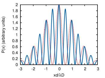
Figure 3: Double-slit interference pattern of the biphoton given by (18), where $\lambda$ is the wavelength of the photons (solid line). Fringe width is $w={(\lambda/2)D\over d}$. Double-slit interference pattern of the photons given by (20) (dotted line). Fringe width is $w={\lambda D\over d}$. A typical profile of $f(x)$ has been used for the plots.

3.3 Single photon interference

We now investigate the possibility of a photon of the entangled pair behaving like a standalone quanton. This can be achieved by fixing detector D2 at $x_{2}=0$ and counting photons by D1 at various $x_{1}$, in coincidence with D2. Putting $x_{2}=0$ corresponds to $r=x_{1}/2$ and $q=x_{1}/2$. Doing that simplifies (LABEL:finalstate) to

$$\Psi(x_{1},x_{2}=0,t) \approx C_{t}\left(e^{{\pi\imath\over 2\lambda D}(x_{1}-d)^{2}}e^{{\pi\imath\over 2\lambda D}x_{1}^{2}}f^{2}(\tfrac{x_{1}}{2})\right.$$ (19)

$$\left.+e^{{\pi\imath\over 2\lambda D}(x_{1}+d)^{2}}e^{{\pi\imath\over 2\lambda D}x_{1}^{2}}f^{2}(\tfrac{x_{1}}{2})\right),$$

where the combined state $\Psi(x_{1},x_{2},t)$ is labeled by the original coordinates $x_{1},x_{2}$, and not by $r,q$. The probability density to find a photon at $x_{1}$, $P(x_{1})$ is given by $P(x_{1})=|\Psi(x_{1},x_{2}=0,t)|^{2}$, and has the following form:

$$P(x_{1}) = |C_{t}|^{2}\epsilon^{2}f^{2}(\tfrac{x_{1}}{2})\left[1+\cos\left({2\pi x_{1}d\over\lambda D}\right)\right].$$ (20)

The above represents a Young’s double-slit interference pattern with a fringe with $w={\lambda D\over d}$. In this arrangement the photons detected by D1 behave as independent quantons with wavelength $\lambda$ (see Figure 3).

4 Conclusions

We have a done a wave-packet analysis of two entangled photons passing through a double-slit. We have shown that the two photons can behave like a single quanton of half the wavelength of the photons when detected in coincidence at the same position. This is in agreement of an earlier analysis and experiment by Fonseca, Monken and Pádua [7]. Going further, we have shown that the two photons can continue to behave like a single quanton even when they are widely separated in space, a highly nonlocal feature. This work extends the theoretical ideas of multiphoton wave packets [6, 7] to a nonlocal scenario. Our result implies that even when two entangled photons are separated in space, they may act like a single quanton which interferes with itself. Entangled particles show very strange and counter-intuitive properties. It has previously been shown that entangled photons can exhibit a nonlocal wave-particle duality [16].

References

- [1] Bohr N. The quantum postulate and the recent development of atomic theory. Nature 1928; 121(3050): 580–590. doi:10.1038/121580a0
- [2] Jönsson C. Electron diffraction at multiple slits. American Journal of Physics 1974; 42(1): 4–11. doi:10.1119/1.1987592
- [3] Nairz O, Arndt M, Zeilinger A. Quantum interference experiments with large molecules. American Journal of Physics 2003; 71(4): 319–325. doi:10.1119/1.1531580
- [4] Bunge M. Foundations of Physics. Springer Tracts in Natural Philosophy, vol. 10, New York: Springer, 1967. doi:10.1007/978-3-642-49287-7
- [5] Lévy-Leblond J-M. Quantum words for a quantum world. In: Epistemological and Experimental Perspectives on Quantum Physics. Greenberger D, Reiter WL, Zeilinger A (editors), Vienna Circle Institute Yearbook, vol. 7, Dordrecht: Springer, 1999, pp. 75–87. doi:10.1007/978-94-017-1454-9_5
- [6] Jacobson J, Björk G, Chuang I, Yamamoto Y. Photonic de Broglie waves. Physical Review Letters 1995; 74(24): 4835–4838. doi:10.1103/PhysRevLett.74.4835
- [7] Fonseca EJS, Monken CH, Pádua S. Measurement of the de Broglie wavelength of a multiphoton wave packet. Physical Review Letters 1999; 82(14): 2868–2871. doi:10.1103/PhysRevLett.82.2868
- [8] Einstein A, Podolsky B, Rosen N. Can quantum-mechanical description of physical reality be considered complete? Physical Review 1935; 47(10): 777–780. doi:10.1103/PhysRev.47.777
- [9] Qureshi T. Understanding Popper’s experiment. American Journal of Physics 2005; 73(6): 541–544. arXiv:quant-ph/0405057, doi:10.1119/1.1866098
- [10] Qureshi T. Popper’s experiment: a modern perspective. Quanta 2012; 1(1): 19–32. doi:10.12743/quanta.v1i1.8
- [11] Chan KW, Torres JP, Eberly JH. Transverse entanglement migration in Hilbert space. Physical Review A 2007; 75(5): 050101. arXiv:quant-ph/0608163, doi:10.1103/PhysRevA.75.050101
- [12] Di Lorenzo Pires H, van Exter MP. Near-field correlations in the two-photon field. Physical Review A 2009; 80(5): 053820. doi:10.1103/PhysRevA.80.053820
- [13] Dillon G. Fourier optics and time evolution of de Broglie wave packets. European Physical Journal Plus 2012; 127(6): 66. arXiv:1112.1242, doi:10.1140/epjp/i2012-12066-2
- [14] D’Angelo M, Chekhova MV, Shih Y. Two-photon diffraction and quantum lithography. Physical Review Letters 2001; 87(1): 013602. arXiv:quant-ph/0103035, doi:10.1103/PhysRevLett.87.013602
- [15] Waitz M, Metz D, Lower J, Schober C, Keiling M, Pitzer M, Mertens K, Martins M, Viefhaus J, Klumpp S, Weber T, Schmidt-Böcking H, Schmidt LPH, Morales F, Miyabe S, Rescigno TN, McCurdy CW, Martín F, Williams JB, Schöffler MS, Jahnke T, Dörner R. Two-particle interference of electron pairs on a molecular level. Physical Review Letters 2016; 117(8): 083002. arXiv:1607.07275, doi:10.1103/PhysRevLett.117.083002
- [16] Siddiqui MA, Qureshi T. A nonlocal wave-particle duality. Quantum Studies: Mathematics and Foundations 2016; 3(1): 115–122. arXiv:1406.1682, doi:10.1007/s40509-015-0064-4