Quantum phase transitions and collective enhancement of level density in odd-$A$ and odd-odd nuclei

Abstract

The nuclear shell model assumes an effective mean-field plus interaction Hamiltonian in a specific configuration space. We want to understand how various interaction matrix elements affect the observables, the collectivity in nuclei and the nuclear level density for odd-$A$ and odd-odd nuclei. Using the $sd$ and $pf$ shells, we vary specific groups of matrix elements and study the evolution of energy levels, transition rates and the level density. In all cases studied, a transition between a “normal” and a collective phase is induced, accompanied by an enhancement of the level density in the collective phase. In distinction to neighboring even-even nuclei, the enhancement of the level density is observed already at the transition point. The collective phase is reached when the single-particle transfer matrix elements are dominant in the shell model Hamiltonian, providing a sign of their fundamental role.

1 Introduction

In the framework of the nuclear shell model, an effective Hamiltonian is used in order to describe the nuclear properties in a certain region of the nuclear chart. The Hamiltonian can be derived either from a theory of a deeper level or by a phenomenological fit to experimental data; in practice one often has to combine these approaches. The good agreement with the data has rendered the shell model a powerful tool of nuclear spectroscopy.

The spectroscopic predictions in the framework of the shell model come from the large-scale diagonalization. Practical necessity to truncate the orbital space may require the corresponding renormalization of the interaction and transition operators. The truncation limits the excitation energy below which the shell model predictions can be reliable (even if we leave aside the continuum decay thresholds). However, the practically useful region in many cases already covers the excitations relevant for laboratory experiments and for astrophysical reactions. The shell model also correctly predicts statistical properties of nuclear states. Therefore it was used as a testing ground for many-body quantum chaos [1]. In the following, we explore the effects of specific components of the effective shell-model interactions on the properties of nuclear spectra, and identify the patterns related to the effects of certain parts of these interactions. In particular, we study the qualitative changes of nuclear observables similar to phase transitions which appear as a function of the interaction in the same shell-model framework. In this way we expect to better understand the relationship between the input effective Hamiltonian and the nuclear output.

The nuclear level density given by the shell model is sensitive to the specific features of the interaction. There are successful applications of the shell model to the prediction of the level density which is a necessary ingredient for the physics of nuclear reactions [2, 3, 4, 5, 6, 7]. The traditional Fermi-gas models are based on the combinatorics of particle-hole excitations near the Fermi level [8, 9, 10], with the resulting level density growing exponentially with energy. In order to account for the effects of pairing [11, 12] or other interactions of collective nature [13, 14], various semi-phenomenological or more elaborate self-consistent mean-field approaches [15, 16] have been developed. The shell model Monte Carlo approach, for example [17], is close in spirit with the shell model, but may have problems with specific interactions and keeping exact quantum numbers. The shell model Hamiltonian inherently includes pairing and other collective interactions. Along with that, matrix elements describing incoherent collision-like processes are present as well. Taking them into account consistently, we come to the level density that, in agreement with data, is a smooth function of excitation energy. Being still limited by truncated space, this approach does not require prohibitively large diagonalization. The regular calculation of the first statistical moments of the Hamiltonian is sufficient for reproducing the realistic level density.

In this work we study the evolution of simple nuclear characteristics under the variation of the values of certain groups of matrix elements in order to link these matrix elements to the emergence of collective effects in nuclei. This work can be considered as an extension of [18] where we limited ourselves to even-even isotopes. Here we study the behavior of odd-$A$ and odd-odd nuclei in the same mass regions under the variation of interactions. This provides an additional insight on how the presence of unpaired fermions affects the changes of nuclear spectral observables and the level density. As will be seen, the effects of the variation of the matrix elements in nuclei with unpaired fermions change the nuclear observables in a strong and systematic way. As a result of the shift of rotational and vibrational excitations to lower energy, the level density reveals the collective enhancement.

2 Matrix elements responsible for collectivity

In the case of the $sd$ shell-model space, there are three single-particle levels (orbitals), $1s_{1/2},0d_{5/2},0d_{3/2}$, and 63 matrix elements of the residual two-body interaction allowed by angular momentum and isospin conservation. Similarly, for the $pf$ shell, there are four single-particle levels, $0f_{7/2},1p_{3/2},0f_{5/2},1p_{1/2}$, and 195 matrix elements of the two-body interaction. The two-body matrix elements naturally fall into three categories labeled by $\delta=0,1,2$ depending on how many particles (zero, one or two) change their orbitals as a result of the interaction process. We will show that a special role defining the mean-field shape is played by the “one unit change”, $\delta=1$, matrix elements.

It is known [20, 21] that even a random (but keeping in force angular momentum and isospin symmetry) set of matrix elements in a finite orbital space results in the energy spectrum and properties of stationary states which carry certain analogies to realistic nuclei. This is essentially a manifestation of the Fermi statistics and symmetry properties of the orbital space for a given particle number with averaging over multiple interaction acts. Artificially changing the reduced matrix elements $-$ intensifying some interaction processes and weakening others $-$ one can find the interaction landscape responsible for specific features of individual nuclei or their groups.

In a recent study [22] conducted in the shell-model space $0f_{7/2},1p_{3/2}$, the matrix elements allowed in this space were varied randomly in order to identify those realizations of the random interaction ensemble which give rise to prolate axial deformation. Among the matrix elements involved, those most important are the $\delta=1$ matrix elements, which are responsible for the mixing of different single-particle spherical orbitals of the same parity $(|\Delta\ell|=2)$ in the process of quadrupole deformation. Taking this result into account, the authors in [18] separated the interaction Hamiltonian into two parts, one containing the $\delta=1$ matrix elements and another one for the remaining matrix elements. By varying the relative strength of matrix elements of these groups, a quantum phase transition was found in even-even nuclei, both in the $sd$ and $pf$ spaces, namely a transition from spherical to deformed shape. The signals of the transition are the regularities of the lowest yrast energies, including the energy ratio $R_{4/2}$, the reduced $B$(E2) transition probabilities between these levels, and the amplitudes of the components of the wave functions.

The deformed phase was realized when the $\delta=1$ matrix elements dominated the Hamiltonian, while the spherical phase arose when the values of these matrix elements decreased with a simultaneous increase of other matrix elements. (In a simplified form, similar phase transformations are known in the interacting boson model [23].) For even-even nuclei, a clear enhancement of the low-energy level density was found in the stable deformed phase compared to the spherical phase, but not in the vicinity of the transitional point where the shape fluctuations are essential and various states have complicated wave functions covering both phases. The existence of such fluctuations measured by the growth of the corresponding correlational entropy of the ground state was found earlier [24]. In what follows we explore the effect of the $\delta=1$ matrix elements in odd-$A$ and odd-odd nuclei in the $sd$ and $pf$ shells. With the same approach, we will search for signs of a quantum phase transition.

3 Quantum phase transition

Nuclear structure models have long provided theoretical tools for analyzing quantum phase transitions [24, 25, 26]. Quantum phase/shape transitions usually occur when the Hamiltonian of the system is known to have distinct limiting dynamical symmetries [27, 28, 29, 30, 31, 32], revealed in the observables of the system by varying a control parameter interpolating between the limiting cases. In the framework of the shell model, pairing and other collective effects are integrated in the two-body interaction and the variation of one group of matrix elements with respect to the others is expected to help better understand the role of certain interaction processes in the final properties of nuclear observables.

To be sure that our versions of the shell model using the standard values of interaction matrix elements are quite realistic, we first demonstrate the quality of the description of nuclear data from the results of the full diagonalization for an odd-odd nucleus ²⁶Al with rich experimental information, see Table 1.

Table 1: Experimental energy levels (MeV) and reduced transition probabilities (Weisskopf units, W.u.) compared with the shell-model results using the USD interaction [33] for ²⁶Al.

Theory		Experiment
Energy	J	Energy	J
0.000	5+	0.0	5+
0.081	0+	0.228	0+
0.712	3+	0.417	3+
0.819	1+	1.058	1+
1.326	2+	1.759	2+
1.737	1+	1.851	1+
2.004	1+	2.069	4+
2.010	2+	2.069	2+
2.121	3+	2.071	1+
2.303	4+	2.365	3+
2.325	3+	2.545	3+
$B$(E2/M1: $J\rightarrow J^{\prime}$)		$B$(E2/M1: $J\rightarrow J^{\prime}$)
E2: 3${}_{1}^{+}\rightarrow 5_{1}^{+}$	10.61	E2: 3${}_{1}^{+}\rightarrow 5_{1}^{+}$	8.19 $\pm$ 0.12
M1: 1${}_{1}^{+}\rightarrow 0_{1}^{+}$	1.84	M1: 1${}_{1}^{+}\rightarrow 0_{1}^{+}$	1.5 $\pm$ 0.3
E2: 1${}_{2}^{+}\rightarrow 3_{1}^{+}$	10.49	E2: 1${}_{2}^{+}\rightarrow 3_{1}^{+}$	4.4 $\pm$ 0.8
E2: 2${}_{2}^{+}\rightarrow 0_{1}^{+}$	12.93	E2: 2${}_{2}^{+}\rightarrow 0_{1}^{+}$	12.6 $\pm$ 2.4

Simulating the quantum phase transition in the shell-model framework, we use now a Hamiltonian of the form,

$$H=h+(1-\lambda)V_{1}+\lambda V_{2},$$ (1)

where $h$ contains the single-particle energies, which will be kept fixed, and $\lambda$ is the control parameter that varies the values of the $\delta=1$ matrix elements, $V_{1}$, and the remaining ($\delta=0$ and 2) matrix elements, $V_{2}$. Varying $\lambda$ from 0 to 1 in steps of 0.1, we study the evolution of observables revealed in the chosen $sd$ (odd-odd and odd-$A$), and $pf$ (odd-odd) nuclei. The results are depicted in Figs. 1-6, 8 and Tables 2-7, with Tables 3-7 found in the Appendix Section. We have checked that keeping $h$ constant while varying the other terms of the Hamiltonian, doesn’t affect the qualitative results.

In even-even nuclei the $\lambda$ dependence of the energies presents a minimum just for the first few yrast low-energy levels. A similar behavior was seen in pairing phase transitions analyzed through the specially constructed entropy [24].

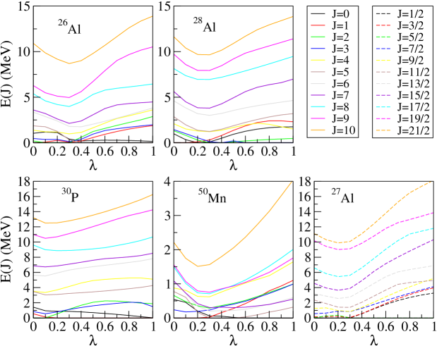
Figure 1: Yrast energies of $J$=0$-$10 in ^26,28Al, ³⁰P, ⁵⁰Mn. and $J$=1/2$-$21/2 in ²⁷Al, as a function of $\lambda$.

In contrast to that, here the minimum persists up to high energy values. For yrast, Fig. 1, as well as for the first ten energy levels with specific spin values, Fig. 2, there is a clear minimum of the level energy for all nuclei studied. For all aluminum isotopes and the $pf$-shell nucleus ⁵⁰Mn, the minimum is around $\lambda\cong$ 0.2$-$0.4, while for ³⁰P the minimum is at $\lambda\cong$ 0.1. In odd-$A$ and odd-odd nuclei, depending on the value of $\lambda$, even the ground state spin can change, showing that the low-energy structure of these nuclei is sensitive to the changes of the important matrix elements. This differs from the even-even nuclei, which for the majority of cases keep the characteristic 0⁺$-$2⁺$-$4⁺ yrast energy sequence in the process of evolution. The shape phase transition differs from the pairing case in putting its more efficient imprint up to higher energies.

To check how the single–particle energies affect this result we repeated the calculations after decreasing or increasing the spacings between them. For example, in one case we reduced these spacings by a factor 1/2, while in another one we increased them by a factor $1.5$. We found that there is always a minimum at a critical value of $\lambda$ which persists for all calculated excited states. The displacement of single–particle energies affects slightly the position of the minimum of energies as a function of $\lambda$. With smaller spacings, the mixing by the $\delta=1$ interaction is effectively stronger, and the original (supposedly deformed) phase survives longer, the phase transition (minimum) appears at larger values of $\lambda$. For instance, in ²⁶Al the minimum of the energies appears closer to $\lambda\cong 0.4$ instead of $\lambda\cong 0.3$, while when the single–particle energies are rarefied, the minimum appears earlier, for smaller $\lambda$ value ($\lambda\cong 0.2$).

Figure 2: The first ten energy levels of $J$=4, as a function of $\lambda$ for ^26,28Al, ³⁰P, ⁵⁰Mn, and $J$= 7/2 for ²⁷Al.

Another indicator of the phase transition is the behavior of the multipole transition probabilities. In Fig. 3 the reduced transition probabilities $B$(E2;$2^{+}_{1}\rightarrow 0^{+}_{1})$, $B$(E2;$2^{+}_{1}\rightarrow 1^{+}_{1})$, $B$(E2;$6^{+}_{1}\rightarrow 4^{+}_{1})$ in ^26,28Al, ³⁰P and $B$(E2;$(5/2)^{+}_{1}\rightarrow(1/2)^{+}_{1})$, $B$(E2;$(3/2)^{+}_{1}\rightarrow(1/2)^{+}_{1})$, $B$(E2;$(7/2)^{+}_{1}\rightarrow(3/2)^{+}_{1})$ in ²⁷Al are presented. In all cases there is a maximum of the transition rate in the region where the signal of a phase transition appears in energies. The probabilities $B$(E2;$2^{+}_{1}\rightarrow 0^{+}_{1})$ for ²⁶Al and $B$(E2;$6^{+}_{1}\rightarrow 4^{+}_{1})$ for ³⁰P have a maximum at slightly greater values of $\lambda$.

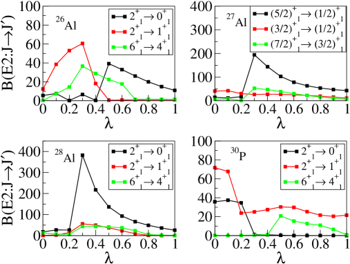
Figure 3: Reduced quadrupole transition probabilities as a function of $\lambda$ for ^26,27,28Al and ³⁰P.

The proton and neutron spin decomposition of the wave functions of different stationary states also presents signs of a quantum phase transition. While this characteristic extends up to highly excited levels, here we show the decomposition of the wave function of the $1^{+}_{1}$ state that serves as the ground state for some values of $\lambda$ in all studied nuclei. In Fig. 4 we have selected to show only those components which have an amplitude over 10%. Some characteristics are common for all nuclei. First, there is an abrupt change of the spin decomposition at the transition point. Second, before the transitional point, there is a strong mixing of the wave function components, while after the transitional point there are one or two dominant components, with the rest falling to a minuscule contribution. For example, for ²⁶Al and $\lambda\leq 0.2$, the $1^{+}_{1}$ state is mainly made up of protons and neutrons coupled to total angular momentum according to ($J_{n},J_{p}$) = (5/2, 5/2), (1/2, 1/2), (9/2, 9/2) and (3/2, 5/2) with all these combinations contributing almost the same. Just after the transitional point and for $\lambda>0.2$, the picture totally changes. The (5/2, 5/2) combination becomes dominant and stays dominant up to $\lambda=1.0$ while other combinations fall below 5%.

While the general picture is similar for all three aluminum isotopes, the situation is slightly different for ⁵⁰Mn. Before the transitional point, the ground state of this nucleus has a strong mixture of different components, ($J_{n},J_{p}$) = (5/2, 5/2), (7/2, 7/2), (11/2, 11/2), (7/2, 5/2) and (9/2, 11/2). After the transitional point the most contributions fall below 10%, whereas the two dominant branches persist up to $\lambda=1.0$. The main component, again ($J_{n},J_{p}$) = (5/2, 5/2), stays around 50%, while the other one, ($J_{n},J_{p}$) = (7/2, 7/2), reaches 20%.

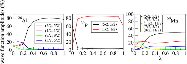
Figure 4: Amplitudes of the wave function 1${}^{+}_{1}$ expanded in terms of proton and neutron angular momenta as a functions of $\lambda$ for ²⁶Al, ³⁰P, and ⁵⁰Mn.

The strong mixture of different spin components in the studied wave functions before the transitional point, compared to the dominance of some spin components after the transitional point, is related to the occupation of the spherical single-particle (s.p.) orbitals. Indeed, one can see a small, but observable difference at the occupation numbers of the s.p. levels in the 1${}^{+}_{1}$ states for all cases. For ²⁶Al and ³⁰P, just before the transitional point ($\lambda<0.4$ for ²⁶Al and $\lambda<0.1$ for ³⁰P), the proton and neutron occupation numbers are ($d_{5/2}$, $s_{1/2}$) $\simeq$ (3.5, 1.1) and ($d_{5/2}$, $s_{1/2}$) $\simeq$ (4.6, 1.8) respectively, with the occupation number of $d_{3/2}$ being always less than 0.5. After the transitional point there is a sudden increase in the occupation number of $d_{5/2}$, accompanied by a decrease in the occupation of $s_{1/2}$, ($d_{5/2}$, $s_{1/2}$) $\simeq$ (4.6, 0.2) and ($d_{5/2}$, $s_{1/2}$) $\simeq$ (5.8, 1.0) for ²⁶Al and ³⁰P, respectively. These changes are relatively small, but apparently sufficient to induce the mixing characteristics observed in the wave functions. Similarly, for ⁵⁰Mn, the occupation numbers of the s.p. levels change from ($f_{7/2}$, $p_{3/2}$, $f_{5/2}$) $\simeq$ (4.6, 0.15, 0.15) before the transition, to ($f_{7/2}$, $p_{3/2}$, $f_{5/2}$) $\simeq$ (4.91, 0.06, 0.03) after the transition, with the $p_{1/2}$ being always less than 0.05. Here from the Nilsson-like occupation scheme we move back to a more normal spherical shell-model occupancy.

In order to find the order of the phase transition we check for discontinuities at the first and second derivatives of the ground state energies. We will discuss all the results, however we will only show pictures of ²⁶Al and ²⁷Al. In the upper panel of Fig. 5 the ground state energies of ²⁶Al and ²⁷Al are plotted, accompanied by the first derivative (middle panel) and second derivative (lower panel) of the ground state energy, as a function of $\lambda$. We see that sudden jumps of the first derivative of the ground state energy produce emphasized minima in its second derivative. Note that here we used steps of 0.01 when moving from $\lambda=0$ to 1 in order to find where the quantum phase transition takes place. The steep minimum of the second derivative of ²⁷Al appears for $\lambda=0.3$, which is exactly the point where we have seen the transitional phenomena. This is analogous for ³⁰P and ⁵⁰Mn, where there is a rather steep minimum of the second derivative of the ground state energy at $\lambda=0.12$ and $\lambda=0.2$, respectively. We can identify these values of $\lambda$ with the phase transition locations.

The situation is slightly different for ^26,28Al, as the second derivative has more than one emphasized minima. These minima correspond to the points where spin of the ground state changes. Only the more pronounced minima, for example for ²⁶Al, those at $\lambda=0.32$ and 0.36, affect the energy behavior, inducing two minima at the energies as a function of $\lambda$. These minima are only observable at the 0.01 step of $\lambda$. For both nuclei the deepest minimum in the energies comes for the largest value of $\lambda$, i.e. for ²⁶Al at $\lambda=0.36$ and for ²⁸Al at $\lambda=0.38$.

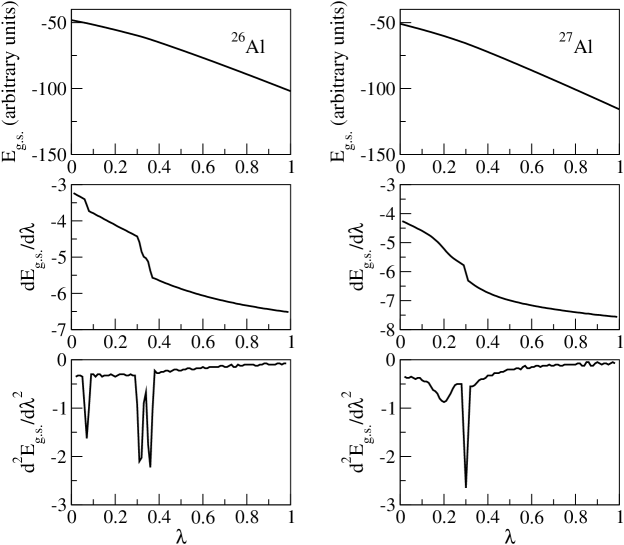
Figure 5: The ground state energy and its first and second derivatives for ²⁶Al and ²⁷Al as a function of $\lambda$.

We look at the wave function, proton and neutron spin decomposition and at the single–particle orbital occupancies to understand the structure of the ground state before and after each spike of its second derivative. Starting with ²⁶Al, before the first minimum, which appears at $\lambda=$0.07, the wave function consists of 10$\%$ contributions of protons and neutrons coupled to angular momenta ($J_{n},J_{p}$) = (5, 5), (1, 1) and (9, 9) and 20$\%$ of (3, 5), (5, 3) components. The single-particle occupancies are ($d_{5/2}$, $s_{1/2}$) $\simeq$ (3.4, 1.1), the $d_{3/2}$ being less than 0.5. After $\lambda=$0.07 and up to the second minimum, the wave function has 10$\%$ contribution of pairs of protons and neutrons with spins ($J_{n},J_{p}$) = (5, 5), (3, 5) and (5, 3) and 15$\%$ of spins (1, 5), (5, 1). The single-particle occupancies change to ($d_{5/2}$, $s_{1/2}$) $\simeq$ (4.0, 0.8), again with a small $d_{3/2}$ component. Thus, the ground state is still highly mixed after the first minimum. The situation considerably changes after the second minimum. There, the ground state wave function suddenly consists mainly (60$\%$) of ($J_{n},J_{p}$) = (5, 5), while the $d_{5/2}$ occupation rises to 4.4, leaving the other two orbitals with less than 0.5 occupation numbers. After the second minimum the contribution of ($J_{n},J_{p}$) = (5, 5) protons and neutrons continues to rise reaching 70$\%$, followed by a rise to 4.6 of the $d_{5/2}$ occupation number. Therefore, the $\lambda$ value 0.32 is the point where the ground state structure changes from mixed to pure configuration.

The case of ²⁸Al, with two minima at $\lambda=$ 0.17 and 0.28 is similar to ²⁶Al, the ground state wave function changing its character from mixed to pure. Before the first minimum, the components of the wavefunction are a mixture of ($J_{n},J_{p}$) = (5, 5), (1, 1) at 20$\%$ and ($J_{n},J_{p}$) = (1, 3), (5, 3) at 10$\%$, the proton occupation numbers being ($d_{5/2}$, $s_{1/2}$) = (3.9, 0.7) and the neutron ($d_{3/2}$, $d_{5/2}$, $s_{1/2}$) = (0.6, 5.2, 1.2). Passing the first minimum, only two components of the wave function become important, the ($J_{n},J_{p}$) = (5, 5), (1, 1) at 55$\%$ and 33$\%$, respectively, with an accompanying sudden increase in the $d_{5/2}$ proton occupancy, ($d_{5/2}$, $s_{1/2}$) = (4.2, 0.6) and the $s_{1/2}$ neutron occupancy, ($d_{5/2}$, $s_{1/2}$) = (5.1, 1.5), with the $d_{3/2}$ occupation number falling below 0.5. After the second minimum a highly pure ground state is formed, having protons and neutrons mainly coupled to ($J_{n},J_{p}$) = (1, 5) at 80$\%$ with the protons mainly occupying the $d_{5/2}$ orbital ($d_{5/2}$ = 4.6) and neutrons mainly occupying the $d_{5/2}$ and less the $s_{1/2}$ ($d_{5/2}$, $s_{1/2}$ = 5.6, 1.0).

Trying to see how deformation changes as a function of $\lambda$, we calculate the quadrupole moment for ^26,28Al, ³⁰P with the results also shown in Fig. 6. It is apparent that the details of the interaction change abruplty the quadrupole moment which behaves differently in those three nuclei. However, in all cases, at the point where the ground state changes its character from mixed to pure, the quadrupole moment has its maximum value, droping to smaller values for $\lambda$ closer to 1. Therefore, the general trend is that, for $\lambda$ values closer to one, the deformation is snaller than for $\lambda$ values close to zero.

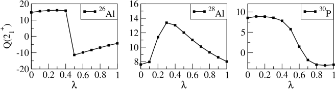
Figure 6: Quadrupole moments for ²⁶Al, ²⁸Al and ³⁰P as a function of $\lambda$.

Summarizing, the results for the energy levels, multipole transition probabilities, the wave function decomposition in proton and neutron spin components, and the quadrupole moments reveal the same coherent picture. At some critical value of $\lambda$, all nuclei undergo a transition from a mixed and collectively deformed phase to a phase close to the spherical shape for larger values of $\lambda$. The yrast, and especially the excited, states of the spectrum show that, for the values of $\lambda$ before the phase transition, the spectrum is overall compressed to lower energies, while, for larger values of $\lambda$, the spectrum expands to higher energies. For example, looking at Fig. 2, at $\lambda\leq 0.3$, the first ten 4⁺ states of ²⁶Al have energies below 3 MeV, but for $\lambda>0.3$ the 4⁺ levels shift considerably higher in energy, finally expanding from 3 to 8 MeV for $\lambda$ = 1.0, when the simple Nilsson-type mixing of single-particle orbitals is excluded. The study of the derivatives of the ground state wave function suggests that this is a second order phase transition.

There is a principal difference between the nuclear models, mainly algebraic, where the quantum phase transitions are studied, and the framework we used to induce a quantum phase transition. In the first case, a system is moving between two well defined symmetries, while in our case the two groups of matrix elements are not directly related to any explicit symmetry. The results, though, show clear signs of a qualitative change in all studied observables of nuclei, as a function of $\lambda$. There is no unique critical value of $\lambda$ where this qualitative change takes place, as the interaction affects different nuclei differently. However we clearly see a coherent behavior of various observables in different nuclei.

4 Level density

To evaluate the level density up to high excitation energy we use the moments method in its current form [6, 7] which is based on our knowledge that the density of states for an individual partition is close to a Gaussian [2, 3, 9]. For a shell-model Hamiltonian that contains a mean-field part and a residual two-body interaction, the total level density is found by summing the contributions of all interacting partitions using Gaussians:

$$\rho(E;\alpha)=\sum_{p}D_{\alpha p}G_{\alpha p}(E).$$ (2)

In this expression, $\alpha$ combines the quantum numbers of spin, isospin and parity, while $p$ numbers partitions (various distributions of fermions over single-particle orbitals); $D_{\alpha p}$ is the dimension of a given partition and $G_{\alpha p}$ is a finite-range Gaussian, defined as

$$G_{\alpha p}=G(E-E_{\alpha p}+E_{g.s.};\sigma_{\alpha p}),$$ (3)

where

$$G(x;\sigma)=C\begin{cases}e^{-x^{2}/2\sigma^{2}},&|x|\leq\eta\sigma,\\ 0,&|x|>\eta\sigma.\end{cases}$$ (4)

Here, $C$ is the normalizing factor, $\int dx\ G(x;\sigma)=1$, and $\eta$ is a finite-range cut-off parameter [4], whose value for this study is set to 2.8. The characteristics of the finite range Gaussians are determined by the ground state energy $E_{g.s.}$ and the moments (traces) of the considered Hamiltonian.

For a given partition, the first moment of the Hamiltonian is the centroid, $E_{\alpha p}$, the mean diagonal matrix element,

$$E_{\alpha p}=\left<H\right>_{\alpha p}=\frac{1}{D_{\alpha p}}{\rm Tr}^{(\alpha p)}H.$$ (5)

The second moment is the dispersion of the Gaussian, $\sigma_{\alpha p}$,

$$\sigma_{\alpha p}^{2}=\left<H^{2}\right>_{\alpha p}-E_{\alpha p}^{2}=\frac{1}{D_{\alpha p}}{\rm Tr}^{(\alpha p)}H^{2}-E_{\alpha p}^{2}.$$ (6)

This is where the mixing of the partitions, due to the interaction processes, is accounted for. The calculation of the moments is done directly by the Hamiltonian matrix, thus avoiding large matrix diagonalizations.

The total level density found by the moments method is in good agreement with the results of the full shell-model calculations. This is illustrated by the example of Fig. 7. For more details on the moments method, as well as comparison with shell model calculations, experimental results, and Fermi-gas phenomenology, we refer to the previous publications [5, 6, 7].

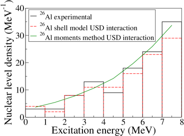
Figure 7: Comparison of experimental nuclear level density (black stair line) with the density calculated by full shell-model diagonalization, using the original parameters of the interaction (red dashed stair line), and through moments method (solid green line) for ²⁶Al, $J$=0$-$7 and positive parity.

Through the modification of the level density, the highly excited states keep memory of the phase transition that happened at lower energy and transmitted pronounced effects high along the spectrum. The behavior of the level density as a function of $\lambda$ is different from the case of even-even nuclei [18]. There the level density was falling as a function of $\lambda$, though there was a clear enhancement of the level density for the cases with the deformed nuclear spectra compared to the vibrational ones. Also, the behavior of the level density did not change when considering higher energy states. In the current study, the level density increases up to the transitional point and then decreases strongly till $\lambda$ = 1.0. In Fig. 8 and Table 2, not only do we observe the enhancement of the level density in the collective phase of the nuclear system, but we also find the signs of collective enhancement at the transitional point itself.

The number of levels was calculated using the moments method for excitation energy up to 10 MeV and spins $J=0-10$ for ^26,28Al and ³⁰P, $J=1/2-21/2$ for ²⁷Al, and excitation energy up to 60 MeV and $J=0-10$ for ⁵⁰Mn. The results, being independent of the angular momentum, do depend on the selected excitation energy. For example, if one calculates the cumulative number of levels of the $sd$ nuclei for excitation energy less than 10 MeV, for some cases (in this study for ²⁷Al, ³⁰P), the behavior of the level density turns out to be different from the one described before. Instead of increasing up to the transitional point and decreasing after that, the level density experiences a continuous decrease as the values of $\lambda$ increase. This decrease, however, is slow up to the transition and much more abrupt just after the transition occurs. The situation is similar for ⁵⁰Mn where the level density is continuously decreasing for any excitation energy below 60 MeV, however the decrease is smooth before the transition and more sharp after that.

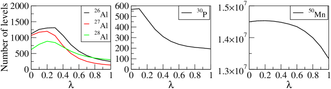
Figure 8: Number of levels up to 10 MeV for ^26,28Al and ³⁰P, for $J$=0$-$10 and $J$=1/2$-$21/2 for ²⁷Al, and up to 60 MeV and $J$=0$-$10 for ⁵⁰Mn.

Table 2: Cumulative number of levels (NoL) with $J$= 0$-$10 up to energy 10 MeV for different values of $\lambda$ for ^26,28Al, ³⁰P, with $J$= 1/2$-$21/2 up to energy 10 MeV for ²⁷Al, and $J$= 0$-$10 up to energy 60 MeV for ⁵⁰ Mn.

$\lambda$	26Al	27Al	28Al	30P	50Mn
0.0	1122	1069	625	567	1.449*107
0.1	1260	1170	789	573	1.452*107
0.2	1303	1199	887	474	1.453*107
0.3	1311	1062	845	378	1.451*107
0.4	1069	744	706	310	1.448*107
0.5	776	500	570	265	1.442*107
0.6	572	345	472	236	1.434*107
0.7	436	251	404	219	1.419*107
0.8	348	194	358	208	1.399*107
0.9	290	159	326	202	1.371*107
1.0	250	137	304	194	1.334*107

In this study, the phase transition is not limited to the ground state and the first few excited levels, but it persists up to the very end of the calculated spectrum. The persistence of the signs of the phase transition from the ground state up to high excitation energy, revealed from the behavior of the excited energy levels and the level density, indicates the proliferation of signatures of the quantum phase transition beyond the ground state. In distinction to the pairing phase transition that is very clear in the ground and pair-vibration states [24] but disappears or becomes a very smooth crossover in excited states of a small Fermi-system [34], here many excited states evolve similarly to the ground state showing essentially the restructuring of the whole mean field. The extension of the quantum phase transition description to high degrees of excitation has been under extensive research for various many-body models [35, 36, 37, 38, 39]. This is the first indication of an excited quantum phase transition in the framework of the shell model.

5 Discussion

In this paper, we studied the evolution of the nuclear observables under the variation of the values of the matrix elements of the shell-model Hamiltonian, keeping the exact global symmetries unchanged. Using the two-body residual interaction, we divided the Hamiltonian into two parts, one containing the “one unit change”, $\delta=1$, matrix elements, and one containing the rest of two-body matrix elements. By varying the entrees of the first group in counterphase to the others, we search for the resulting behavior of observables in various nuclei.

The nuclei studied were odd-$A$ (²⁷Al) and odd-odd, with either the same (²⁶Al, ³⁰P, ⁵⁰Mn) or different (²⁸Al) number of valence protons and neutrons. We concentrated on the signals of evolution in the energy spectrum and transition probabilities, the structure of the stationary wave functions, and the level density in order to search for the signs of coherent behavior dictated by the variation of the effective many-body Hamiltonian.

Earlier [18] the similar instruments were applied to even-even nuclei where it was found that a quantum phase transition occurs in the structure of the first yrast levels, namely the transformation between rotational and vibrational phases as it was possible to conclude from the evolution of typical observables. In the current case, a transition between a collective and a non-collective phase is more pronounced. The $\delta=1$ matrix elements are indeed carriers of collectivity, acting more strongly on unpaired fermions. As a result, this transition extends up to the whole spectrum, providing evidence of the collective enhancement in the level density. This is seen already at the transitional point being preformed by the unpaired and freely interacting particles. In this group of nuclei, the first example of an excited-state quantum phase transition is found in the shell-model framework.

From a slightly more general viewpoint, we open the door into the “kitchen” of the large-scale shell-model diagonalization where usually only the final results are discussed and compared to the experiment, while the interplay of different trends remains hidden in the computations. Meanwhile, looking at the role of individual players representing various physical components of the interacting system can be a useful additional source of information about many-body physics.

Appendix A. Tables

Table 3: Yrast energies of $0^{+}$$-$$10^{+}$ (MeV) for ²⁶Al as a function of $\lambda$.

$\lambda$	$0^{+}_{1}$	$1^{+}_{1}$	$2^{+}_{1}$	$3^{+}_{1}$	$4^{+}_{1}$	$5^{+}_{1}$	$6^{+}_{1}$	$7^{+}_{1}$	$8^{+}_{1}$	$9^{+}_{1}$	$10^{+}_{1}$
0.0	1.038	0.000	0.190	0.466	1.368	1.854	3.355	3.595	5.373	6.268	10.907
0.1	1.182	0.075	0.000	0.357	1.206	1.754	2.877	3.206	4.598	5.485	9.861
0.2	1.117	0.258	0.000	0.361	1.177	1.251	2.391	2.616	4.198	5.114	9.176
0.3	0.408	0.062	0.000	0.129	0.973	0.331	1.793	2.126	3.979	4.962	8.691
0.4	0.191	0.183	0.599	0.379	1.135	0.000	1.749	2.384	4.497	5.609	9.005
0.5	0.254	0.577	1.234	0.951	1.639	0.000	2.041	3.073	5.309	6.727	9.799
0.6	0.280	0.930	1.576	1.344	2.159	0.000	2.358	3.756	5.778	7.920	10.695
0.7	0.278	1.238	1.905	1.538	2.656	0.000	2.700	4.155	5.977	9.022	11.649
0.8	0.253	1.499	2.216	1.701	2.955	0.000	3.062	4.301	6.124	9.669	12.602
0.9	0.208	1.711	2.510	1.846	3.274	0.000	3.436	4.393	6.278	10.160	13.352
1.0	0.144	1.876	2.786	1.973	3.607	0.000	3.817	4.477	6.448	10.520	13.896

Table 4: Yrast energies of $1/2^{+}$$-$$21/2^{+}$ (MeV) for ²⁷Al as a function of $\lambda$.

$\lambda$	${1/2}^{+}_{1}$	${3/2}^{+}_{1}$	${5/2}^{+}_{1}$	${7/2}^{+}_{1}$	${9/2}^{+}_{1}$	${11/2}^{+}_{1}$	${13/2}^{+}_{1}$	${15/2}^{+}_{1}$	${17/2}^{+}_{1}$	${19/2}^{+}_{1}$	${21/2}^{+}_{1}$
0.0	0.000	0.152	0.038	0.562	1.269	2.365	3.209	4.559	6.593	10.177	11.112
0.1	0.000	0.187	0.258	0.647	1.330	1.899	2.878	3.952	5.845	9.427	10.312
0.2	0.000	0.207	0.355	0.894	0.979	1.423	2.568	3.647	5.441	9.007	9.886
0.3	0.003	0.059	0.000	0.836	0.842	1.396	2.752	3.889	5.616	9.118	10.069
0.4	0.560	0.578	0.000	1.265	1.392	2.073	3.612	4.926	6.614	9.850	11.106
0.5	1.195	1.241	0.000	1.780	2.081	2.874	4.539	6.129	7.825	10.783	12.399
0.6	1.787	1.911	0.000	2.295	2.787	3.678	5.436	7.149	9.060	11.791	13.801
0.7	2.291	2.533	0.000	2.790	3.464	4.422	6.060	8.006	10.173	12.538	15.235
0.8	2.701	3.084	0.000	3.260	4.093	4.662	6.371	8.805	11.053	12.966	16.480
0.9	3.025	3.560	0.000	3.705	4.669	4.804	6.632	9.568	11.439	13.403	17.342
1.0	3.275	3.965	0.000	4.122	5.194	4.937	6.886	10.305	11.800	13.863	18.137

Table 5: Yrast energies of $0^{+}$$-$$10^{+}$ (MeV) for ²⁸Al as a function of $\lambda$.

$\lambda$	$0^{+}_{1}$	$1^{+}_{1}$	$2^{+}_{1}$	$3^{+}_{1}$	$4^{+}_{1}$	$5^{+}_{1}$	$6^{+}_{1}$	$7^{+}_{1}$	$8^{+}_{1}$	$9^{+}_{1}$	$10^{+}_{1}$
0.0	0.982	0.000	1.316	1.442	2.086	2.860	4.602	5.623	8.137	9.720	11.636
0.1	0.334	0.000	0.809	0.996	1.511	1.969	3.824	4.493	7.365	8.580	10.394
0.2	0.000	0.102	0.290	0.542	1.297	1.370	3.194	3.839	6.951	7.940	9.690
0.3	0.094	0.307	0.000	0.119	1.211	1.237	3.007	3.801	6.946	7.936	9.651
0.4	0.495	0.795	0.000	0.001	1.377	1.489	3.219	4.264	7.190	8.454	10.154
0.5	0.929	1.361	0.105	0.201	1.678	1.868	3.546	4.936	7.532	9.205	10.901
0.6	1.262	1.849	0.201	0.000	1.964	2.229	3.831	5.612	7.889	9.834	11.693
0.7	1.498	2.218	0.285	0.000	2.148	2.555	4.068	6.090	8.265	10.243	12.408
0.8	1.650	2.404	0.358	0.000	2.018	2.836	4.273	6.373	8.659	10.630	12.941
0.9	1.729	2.403	0.418	0.000	1.763	3.055	4.459	6.595	9.063	11.012	13.400
1.0	1.747	0.880	0.470	0.000	1.514	3.198	4.643	6.980	9.473	11.403	13.856

Table 6: Yrast energies of $0^{+}$$-$$10^{+}$ (MeV) for ³⁰P as a function of $\lambda$.

$\lambda$	$0^{+}_{1}$	$1^{+}_{1}$	$2^{+}_{1}$	$3^{+}_{1}$	$4^{+}_{1}$	$5^{+}_{1}$	$6^{+}_{1}$	$7^{+}_{1}$	$8^{+}_{1}$	$9^{+}_{1}$	$10^{+}_{1}$
0.0	1.418	0.546	0.000	0.839	3.531	3.473	5.643	6.861	9.604	10.986	13.200
0.1	0.947	0.127	0.000	0.559	3.357	3.036	5.528	6.730	8.986	10.491	12.497
0.2	0.879	0.000	0.544	0.804	3.700	3.097	5.929	6.857	8.863	10.698	12.526
0.3	0.865	0.000	1.152	1.119	4.151	3.225	6.306	7.089	8.892	11.105	12.790
0.4	0.798	0.000	1.673	1.380	4.600	3.331	6.561	7.340	8.968	11.554	13.134
0.5	0.701	0.000	2.065	1.596	4.927	3.439	6.755	7.597	9.101	12.031	13.539
0.6	0.590	0.000	2.250	1.776	5.079	3.560	6.935	7.811	9.292	12.524	13.993
0.7	0.469	0.000	2.229	1.932	5.189	3.699	7.118	7.920	9.541	13.023	14.485
0.8	0.333	0.000	2.110	2.074	5.264	3.854	7.311	8.042	9.843	13.478	15.013
0.9	0.172	0.000	1.962	2.036	5.265	4.027	7.519	8.221	10.198	13.838	15.581
1.0	0.030	0.000	1.878	1.502	5.107	4.274	7.807	8.520	10.662	14.238	16.252

Table 7: Yrast energies of $0^{+}$$-$$10^{+}$ (MeV) for ⁵⁰Mn as a function of $\lambda$.

$\lambda$	$0^{+}_{1}$	$1^{+}_{1}$	$2^{+}_{1}$	$3^{+}_{1}$	$4^{+}_{1}$	$5^{+}_{1}$	$6^{+}_{1}$	$7^{+}_{1}$	$8^{+}_{1}$	$9^{+}_{1}$	$10^{+}_{1}$
0.0	0.543	0.000	0.658	0.239	0.877	0.774	1.087	1.083	1.493	1.558	2.213
0.1	0.456	0.000	0.478	0.176	0.810	0.605	0.720	0.729	1.011	1.067	1.746
0.2	0.200	0.000	0.357	0.195	0.631	0.165	0.337	0.417	0.735	0.792	1.511
0.3	0.061	0.026	0.287	0.232	0.620	0.000	0.202	0.305	0.710	0.756	1.562
0.4	0.051	0.158	0.364	0.335	0.761	0.000	0.214	0.316	0.834	0.853	1.795
0.5	0.018	0.277	0.428	0.404	0.892	0.000	0.219	0.305	0.955	0.934	2.051
0.6	0.000	0.421	0.515	0.489	1.023	0.031	0.253	0.316	1.110	1.043	2.364
0.7	0.000	0.592	0.627	0.599	1.129	0.092	0.320	0.355	1.305	1.188	2.733
0.8	0.000	0.794	0.749	0.718	1.238	0.171	0.401	0.396	1.517	1.335	3.122
0.9	0.000	0.935	0.866	0.849	1.438	0.236	0.493	0.471	1.754	1.543	3.576
1.0	0.000	1.101	0.993	0.992	1.642	0.317	0.597	0.550	2.006	1.756	4.042

References

- [1] V. Zelevinsky, B.A. Brown, N. Frazier, and M. Horoi, Phys. Rep. 276, 315 (1996).
- [2] S.S.M. Wong, Nuclear Statistical Spectroscopy (Oxford University Press, 1986).
- [3] V.K.B. Kota and R.U. Haq, eds., Spectral Distributions in Nuclei and Statistical Spectroscopy (World Scientific, Singapore, 2010).
- [4] R.A. Sen’kov and M. Horoi, Phys. Rev. C 82, 024304 (2010).
- [5] R.A. Sen’kov, M. Horoi, and V.G. Zelevinsky, Phys. Lett. B 702, 413 (2011).
- [6] R.A. Sen’kov, M. Horoi, and V.G. Zelevinsky, Computer Physics Communications 184, 215 (2013).
- [7] R.A. Sen’kov and V. Zelevinsky, Phys. Rev. C 93, 064304 (2016).
- [8] H.A. Bethe, Phys. Rev. 50, 332 (1936); Rev. Mod. Phys. 9, 69 (1937).
- [9] T.A. Brody, J. Flores, J.B. French, P.A. Mello, A. Pandey, and S.S.M. Wong, Rev. Mod. Phys. 53, 385 (1981).
- [10] A. Bohr and B.R. Mottelson, Nuclear Structure, Vol. I: Single-Particle Motion (World Scientific, Singapore, 1997).
- [11] S. Goriely, S. Hilaire, and A.J. Koning, Phys. Rev. C 78, 064307 (2008).
- [12] S. Hilaire, M. Girod, S. Goriely, and A.J. Koning. Phys. Rev. C 86, 064317 (2012).
- [13] F.S. Chang, J.B. French, and T.H. Thio, Ann. Phys. 66, 137 (1971).
- [14] G. Hansen and A.S. Jensen, Nucl. Phys. A406, 236 (1983).
- [15] A.V. Ignatyuk, K.K. Istekov, and G.N. Smirenkin, Sov. J. Phys. 29, 450 (1979).
- [16] S. Bjørnholm, A. Bohr, and B.R. Mottelson, Physics and Chemistry of fission 1, 367 (1974), IAEA, Vienna.
- [17] Y. Alhassid, M. Bonett-Matiz, S. Liu, and H. Nakada, Phys. Rev. C 92, 024307 (2015).
- [18] S. Karampagia and V. Zelevinsky, Phys. Rev. C 94, 014321 (2016).
- [19] T. Papenbrock and H.A. Weidenmüller, Nucl. Phys. A757, 422 (2005).
- [20] C.W. Johnson, G.F. Bertsch, and D.J. Dean, Phys. Rev. Lett. 80, 2749 (1998).
- [21] V. Zelevinsky and A. Volya, Phys. Rep. 391, 311 (2004).
- [22] M. Horoi and V. Zelevinsky, Phys. Rev. C 81, 034306 (2010).
- [23] R. Bijker and A. Frank, Phys. Rev. Lett. 84, 420 (2000).
- [24] A. Volya and V. Zelevinsky, Phys. Lett. B 574, 27 (2003).
- [25] A.E.L. Dieperink, O. Scholten, and F. Iachello, Phys. Rev. Lett. 44, 1747 (1980).
- [26] D.H. Feng, R. Gilmore, and S.R. Deans, Phys. Rev. C 23, 1254 (1981).
- [27] H. Chen, J.R. Brownstein, and D.J. Rowe, Phys. Rev. C 42, 1422 (1990).
- [28] C. Bahri, D.J. Rowe, and W. Wijesundera, Phys. Rev. C 58, 1539 (1998).
- [29] D.J. Rowe, Nucl. Phys. A745, 47 (2004).
- [30] Y. A. Luo, F. Pan, T. Wang, P. Z. Ning, and J.P. Draayer, Phys. Rev. C 73, 044323 (2006).
- [31] Y. Luo, Y. Zhang, X. Meng, F. Pan, and J.P. Draayer, Phys. Rev. C 80, 014311 (2009).
- [32] P. Cejnar, J. Jolie, and R.F. Casten, Rev. Mod. Phys. 82, 2155 (2010).
- [33] B.H. Wildenthal, Prog. Part. Nucl. Phys. 11, 5 (1984).
- [34] M. Horoi and V. Zelevinsky, Phys. Rev. C 75, 054303 (2007).
- [35] P. Cejnar, M. Macek, S. Heinze, J. Jolie, and J. Dobeš, J. Phys. A: Math. Gen. 39, L515 (2006).
- [36] M.A. Caprio, P. Cejnar, and F. Iachello, Ann. Phys. 323, 1106 (2008).
- [37] P. Cejnar and J. Jolie, Progr. Part. Nucle. Phys. 62, 210 (2009).
- [38] P. Pérez-Fernández, A. Relaño, J.M. Arias, P. Cejnar, J. Dukelsky, and J.E. García-Ramos, Phys. Rev. E 83, 046208 (2011).
- [39] C.M. Lóbez and A. Relaño, Phys. Rev. E 94, 012140 (2016).