Disentangling weak and strong interactions in $B\to K^{*}(\to K\pi)\pi$ Dalitz-plot analyses

Abstract

Dalitz-plot analyses of $B\rightarrow K\pi\pi$ decays provide direct access to decay amplitudes, and thereby weak and strong phases can be disentangled by resolving the interference patterns in phase space between intermediate resonant states. A phenomenological isospin analysis of $B\rightarrow K^{*}(\rightarrow K\pi)\pi$ decay amplitudes is presented exploiting available amplitude analyses performed at the BABAR, Belle and LHCb experiments. A first application consists in constraining the CKM parameters thanks to an external hadronic input. A method, proposed some time ago by two different groups and relying on a bound on the electroweak penguin contribution, is shown to lack the desired robustness and accuracy, and we propose a more alluring alternative using a bound on the annihilation contribution. A second application consists in extracting information on hadronic amplitudes assuming the values of the CKM parameters from a global fit to quark flavour data. The current data yields several solutions, which do not fully support the hierarchy of hadronic amplitudes usually expected from theoretical arguments (colour suppression, suppression of electroweak penguins), as illustrated from computations within QCD factorisation. Some prospects concerning the impact of future measurements at LHCb and Belle II are also presented. Results are obtained with the CKMfitter analysis package, featuring the frequentist statistical approach and using the Rfit scheme to handle theoretical uncertainties.

I Introduction

Non-leptonic $B$ decays have been extensively studied at the $B$-factories BABAR and Belle Bevan:2014iga , as well at the LHCb experiment Bediaga:2012py . Within the Standard Model (SM) some of these modes provide valuable information on the Cabibbo-Kobayashi-Maskawa (CKM) matrix and the structure of $CP$ violation Cabibbo:1963yz ; Kobayashi:1973fv , entangled with hadronic amplitudes describing processes either at the tree level or the loop level (the so-called penguin contributions). Depending on the transition considered, one may or may not get rid of hadronic contributions which are notoriously difficult to assess. For instance, in $b\rightarrow c\bar{c}s$ processes, the CKM phase in the dominant tree amplitude is the same as that of the Cabibbo-suppressed penguin one, so the only relevant weak phase is the $B_{d}$-mixing phase $2\beta$ (up to a very high accuracy) and it can be extracted from a $CP$ asymmetry out of which QCD contributions drop to a very high accuracy. For charmless $B$ decays, the two leading amplitudes often carry different CKM and strong phases, and thus the extraction of CKM couplings can be more challenging. In some cases, for instance the determination of $\alpha$ from $B\to\pi\pi$ Olivier , one can use flavour symmetries such as isospin in order to extract all hadronic contributions from experimental measurements, while constraining CKM parameters. This has provided many useful constraints for the global analysis of the CKM matrix within the Standard Model and the accurate determination of its parameters Charles:2004jd ; Charles:2015gya ; CKMfitterwebsite ; Koppenburg:2017mad , as well as inputs for some models of New Physics Deschamps:2009rh ; Lenz:2010gu ; Lenz:2012az ; Charles:2013aka .

The constraints obtained from some of the non-leptonic two-body $B$ decays can be contrasted with the unclear situation of the theoretical computations for these processes. Several methods (QCD factorisation Beneke:1999br ; Beneke:2000ry ; Beneke:2003zv ; Beneke:2006hg , perturbative QCD approach Li:2001ay ; Li:2002mi ; Li:2003yj ; Ali:2007ff ; Li:2014rwa ; Wang:2016rlo , Soft-Collinear Effective Theory Bauer:2002aj ; Beneke:2003pa ; Bauer:2004tj ; Bauer:2005kd ; Becher:2014oda ) were devised more than a decade ago to compute hadronic contributions for non-leptonic decays. However, some of their aspects remain debated at the conceptual level DescotesGenon:2001hm ; Ciuchini:2001gv ; Beneke:2004bn ; Manohar:2006nz ; Li:2009wba ; Feng:2009rp ; Beneke:2009az ; Becher:2011dz ; Beneke:2015wfa , and they struggle to reproduce some data on $B$ decays into two mesons, especially $\pi^{0}\pi^{0}$, $\rho^{0}\rho^{0}$, $K\pi$, $\phi K^{*}$, $\rho K^{*}$ Beneke:2015wfa . Considering the progress performed meanwhile in the determination of the CKM matrix, it is clear that by now, most of these non-leptonic modes provide more a test of our understanding of hadronic process rather than competitive constraints on the values of the CKM parameters, even though it can be interesting to consider them from one point of view or the other.

Our analysis is focused on the study of $B\rightarrow K^{*}(\rightarrow K\pi)\pi$ decay amplitudes, with the help of isospin symmetry. Among the various $b\rightarrow u\bar{u}s$ processes, the choice of $B\rightarrow K^{*}\pi$ system is motivated by the fact that an amplitude (Dalitz-plot) analysis of the three-body final state $K\pi\pi$ provides access to several interference phases among different intermediate $K^{*}\pi$ states. The information provided by these physical observables highlights the potential of the $B\rightarrow K^{*}\pi$ system $(VP)$ compared with $B\rightarrow K\pi$ $(PP)$ where only branching ratios and $CP$ asymmetries are accessible. Similarly, the $B\rightarrow K^{*}\pi$ system leads to the final $K\pi\pi$ state with a richer pattern of interferences and thus a larger set of observables than other pseudoscalar-vector states, like, say, $B\to K\rho$ (indeed, $K\pi\pi$ exhibits $K^{*}$ resonances from either of the two combinations of $K\pi$ pairs, whereas the $\rho$ meson comes from the only $\pi\pi$ pair available). In addition, the study of these modes provides experimental information on the dynamics of pseudoscalar-vector modes, which is less known and more challenging from the theoretical point of view. Finally, this system has been studied extensively at the BABAR Aubert:2008bj ; Aubert:2009me ; BABAR:2011ae ; Lees:2015uun and Belle Garmash:2006bj ; Dalseno:2008wwa experiments, and a large set of observables is readily available.

Let us mention that other approaches, going beyond isospin symmetry, have been proposed to study this system. For instance, one can use $SU(3)$ symmetry and $SU(3)$-related channels in addition to the ones that we consider in this paper Bhattacharya:2013boa ; Bhattacharya:2015uua . Another proposal is the construction of the fully SU(3)-symmetric amplitude Bhattacharya:2014eca to which the spin-one intermediate resonances that we consider here do not contribute.

The rest of this article is organised in the following way. In Sec. II, we discuss the observables provided by the analysis of the $K\pi\pi$ Dalitz plot analysis. In Sec. III, we recall how isospin symmetry is used to reduce the set of hadronic amplitudes and their connection with diagram topologies. In Sec. IV, we discuss two methods to exploit these decays in order to extract information on the CKM matrix, making some assumptions about the size of specific contributions (either electroweak penguins or annihilation). In Sec. V, we take the opposite point of view. Taking into account our current knowledge of the CKM matrix from global analysis, we set constraints on the hadronic amplitudes used to describe these decays, and we make a brief comparison with theoretical estimates based on QCD factorisation. In Sec. VI, we perform a brief prospective study, determining how the improved measurements expected from LHCb and Belle II may modify the determination of the hadronic amplitudes before concluding. In the Appendices, we discuss various technical aspects concerning the inputs and the fits presented in the paper.

II Dalitz-plot amplitudes

Charmless hadronic $B$ decays are a particularly rich source of experimental information Bevan:2014iga ; Bediaga:2012py . For $B$ decays into three light mesons (pions and kaons), the kinematics of the three-body final state can be completely determined experimentally, thus allowing for a complete characterisation of the Dalitz-plot (DP) phase space. In addition to quasi-two-body event-counting observables, the interference phases between pairs of resonances can also be accessed, and $CP$-odd (weak) phases can be disentangled from $CP$-even (strong) ones. Let us however stress that the extraction of the experimental information relies heavily on the so-called isobar approximation, widely used in experimental analyses because of its simplicity, and in spite of its known shortcomings Amato:2016xjv .

The $B\rightarrow K\pi\pi$ system is particularly interesting, as the decay amplitudes from intermediate $B\rightarrow PV$ resonances ($K^{\star}(892)$ and $\rho(770)$) receive sizable contributions from both tree-level and loop diagrams, and interfere directly in the common phase-space regions (namely the “corners” of the DP). The presence of additional resonant intermediate states further constrain the interference patterns and help resolving potential phase ambiguities. In the case of $B^{0}\rightarrow K^{+}\pi^{-}\pi^{0}$ and $B^{+}\rightarrow K^{0}_{S}\pi^{+}\pi^{0}$, two different $K^{\star}(892)$ states contribute to the decay amplitude, and their interference phases can be directly measured. For $B^{0}\rightarrow K^{0}_{S}\pi^{+}\pi^{-}$, the time-dependent evolution of the decay amplitudes for $B^{0}$ and $\overline{B^{0}}$ provides (indirect) access to the relative phase between the $B^{0}\rightarrow K^{\star+}\pi^{-}$ and $\overline{B^{0}}\rightarrow K^{\star-}\pi^{+}$ amplitudes.

In the isobar approximation Amato:2016xjv , the total decay amplitude for a given mode is a sum of intermediate resonant contributions, and each of these is a complex function of phase-space: ${\cal A}(DP)=\sum_{i}A_{i}F_{i}(DP)$, where the sum rolls over all the intermediate resonances providing sizable contributions, the $F_{i}$ functions are the “lineshapes” of each resonance, and the isobar parameters $A_{i}$ are complex coefficients indicating the strength of each intermediate amplitude. The corresponding relation is $\overline{{\cal A}}(DP)=\sum_{i}\overline{A_{i}}~{}\overline{F_{i}}(DP)$ for $CP$-conjugate amplitudes.

Any convention-independent function of isobar parameters is a physical observable. For instance, for a given resonance “$i$”, its direct $CP$ asymmetry $A_{CP}$ is expressed as

$$A_{CP}^{i}=\frac{|\overline{A_{i}}|^{2}-|A_{i}|^{2}}{|\overline{A_{i}}|^{2}+|A_{i}|^{2}},$$ (1)

and its partial fit fraction $FF^{i}$ is

$$FF^{i}=\frac{(|A_{i}|^{2}+|\overline{A_{i}}|^{2})\int_{DP}|F_{i}(DP)|^{2}d(DP)}{\sum_{jk}(A_{j}A^{*}_{k}+\overline{A_{j}}~{}\overline{A^{*}_{k}})\int_{DP}F_{j}(DP)F^{*}_{k}(DP)d(DP)}.$$ (2)

To obtain the partial branching fraction ${\cal B}^{i}$, the fit fraction has to be multiplied by the total branching fraction of the final state (e.g., $B^{0}\to K^{0}_{S}\pi^{+}\pi^{-}$),

$${\cal B}^{i}={\it FF}^{i}\times{\cal B}_{incl}.$$ (3)

A phase difference $\varphi_{ij}$ between two resonances “$i$” and “$j$” contributing to the same total decay amplitude (i.e., between resonances in the same DP) is

$$\varphi^{ij}=\arg(A_{i}/A_{j}),\qquad\overline{\varphi}_{ij}=\arg\left(\overline{A_{i}}/\overline{A_{j}}\right)\,,$$ (4)

and a phase difference between the two $CP$-conjugate amplitudes for resonance “$i$” is

$$\Delta\varphi^{i}=\arg\left(\frac{q}{p}\frac{\overline{A_{i}}}{A_{i}}\right)\,,$$ (5)

where $q/p$ is the $B^{0}-\overline{B^{0}}$ oscillation parameter.

For $B\rightarrow K^{\star}\pi$ modes, there are in total 13 physical observables. These can be classified as four branching fractions, four direct $CP$ asymmetries and five phase differences:

• The $CP$-averaged ${\cal B}^{+-}=BR(B^{0}\rightarrow K^{\star+}\pi^{-})$ branching fraction and its corresponding $CP$ asymmetry $A_{CP}^{+-}$. These observables can be measured independently in the $B^{0}\rightarrow K^{0}_{S}\pi^{+}\pi^{-}$ and $B^{0}\rightarrow K^{+}\pi^{-}\pi^{0}$ Dalitz planes.

• The $CP$-averaged ${\cal B}^{00}=BR(B^{0}\rightarrow K^{\star 0}\pi^{0})$ branching fraction and its corresponding $CP$ asymmetry $A_{CP}^{00}$. These observables can be accessed both in the $B^{0}\rightarrow K^{+}\pi^{-}\pi^{0}$ and $B^{0}\rightarrow K^{0}_{S}\pi^{0}\pi^{0}$ Dalitz planes.

• The $CP$-averaged ${\cal B}^{+0}=BR(B^{+}\rightarrow K^{\star+}\pi^{0})$ branching fraction and its corresponding $CP$ asymmetry $A_{CP}^{+0}$. These observables can be measured both in the $B^{+}\rightarrow K^{0}_{S}\pi^{+}\pi^{0}$ and $B^{+}\rightarrow K^{+}\pi^{0}\pi^{0}$ Dalitz planes.

• The $CP$-averaged ${\cal B}^{0+}=BR(B^{+}\rightarrow K^{\star 0}\pi^{+})$ branching fraction and its corresponding $CP$ asymmetry $A_{CP}^{0+}$. They can be measured both in the $B^{+}\rightarrow K^{+}\pi^{+}\pi^{-}$ and $B^{+}\rightarrow K^{0}_{S}\pi^{0}\pi^{+}$ Dalitz planes.

• The phase difference $\varphi^{00,+-}$ between $B^{0}\rightarrow K^{\star+}\pi^{-}$ and $B^{0}\rightarrow K^{\star 0}\pi^{0}$, and its corresponding $CP$ conjugate $\overline{\varphi}^{{00},-+}$. They can be measured in the $B^{0}\rightarrow K^{+}\pi^{-}\pi^{0}$ Dalitz plane and in its $CP$ conjugate DP $\overline{B^{0}}\rightarrow K^{-}\pi^{+}\pi^{0}$, respectively.

• The phase difference $\varphi^{+0,0+}$ between $B^{+}\rightarrow K^{\star+}\pi^{0}$ and $B^{+}\rightarrow K^{\star 0}\pi^{+}$, and its corresponding $CP$ conjugate $\overline{\varphi}^{{-0},0-}$. They can be measured in the $B^{+}\rightarrow K^{0}_{S}\pi^{+}\pi^{0}$ Dalitz plane and in its $CP$ conjugate DP $B^{-}\rightarrow K^{0}_{S}\pi^{-}\pi^{0}$, respectively.

• The phase difference $\Delta\varphi^{+-}$ between $B^{0}\rightarrow K^{\star+}\pi^{-}$ and its $CP$ conjugate $\overline{B^{0}}\rightarrow K^{\star-}\pi^{+}$. This phase difference can only be measured in a time-dependent analysis of the $K^{0}_{S}\pi^{+}\pi^{-}$ DP. As $K^{\star+}\pi^{-}$ is only accessible for $B^{0}$ and $K^{\star-}\pi^{+}$ to $\overline{B^{0}}$ only, the $B^{0}\rightarrow K^{\star+}\pi^{-}$ and $\overline{B^{0}}\rightarrow K^{\star-}\pi^{+}$ amplitudes do not interfere directly (they contribute to different DPs). But they do interfere with intermediate resonant amplitudes that are accessible to both $B^{0}$ and $\overline{B^{0}}$, like $\rho^{0}(770)K^{0}_{S}$ or $f_{0}(980)K^{0}_{S}$, and thus the time-dependent oscillation is sensitive to the combined phases from mixing and decay amplitudes.

II.1 Real-valued physical observables

The set of physical observables described in the previous paragraph (branching fractions, $CP$ asymmetries and phase differences) has the advantage of providing straightforward physical interpretations. From a technical point of view though, the phase differences suffer from the drawback of their definition with a $2\pi$ periodicity. This feature becomes an issue when the experimental uncertainties on the phases are large and the correlations between observables are significant, since there is no straightforward way to properly implement their covariance into a fit algorithm. Moreover the uncertainties on the phases are related to the moduli of the corresponding amplitudes, leading to problems when the latter are not known precisely and can reach values compatible with zero. As a solution to this issue, a set of real-valued Cartesian physical observables is defined, in which the $CP$ asymmetries and phase differences are expressed in terms of the real and imaginary parts of ratios of isobar amplitudes scaled by the ratios of the corresponding branching fractions and $CP$ asymmetries. The new observables are functions of branching fractions, $CP$ asymmetries and phase differences, and are thus physical observables. The new set of observables, similar to the $U$ and $I$ observables defined in $B\to\rho\pi$ Olivier , are expressed as the real and imaginary parts of ratios of amplitudes as follows,

$${\mathcal{R}e}\left(A_{i}/A_{j}\right)=\sqrt{\frac{{\cal B}^{i}}{{\cal B}^{j}}\frac{A_{CP}^{i}-1}{A_{CP}^{j}-1}}\cos(\varphi_{ij})\,,$$ (6)

$${\mathcal{I}m}\left(A_{i}/A_{j}\right)=\sqrt{\frac{{\cal B}^{i}}{{\cal B}^{j}}\frac{A_{CP}^{i}-1}{A_{CP}^{j}-1}}\sin(\varphi_{ij})\,,$$ (7)

$${\mathcal{R}e}\left(\overline{A}_{i}/\overline{A}_{j}\right)=\sqrt{\frac{{\cal B}^{i}}{{\cal B}^{j}}\frac{A_{CP}^{i}+1}{A_{CP}^{j}+1}}\cos(\overline{\varphi}_{ij})\,,$$ (8)

$${\mathcal{I}m}\left(\overline{A}_{i}/\overline{A}_{j}\right)=\sqrt{\frac{{\cal B}^{i}}{{\cal B}^{j}}\frac{A_{CP}^{i}+1}{A_{CP}^{j}+1}}\sin(\overline{\varphi}_{ij})\,.$$ (9)

We see that some observables are not defined in the case $A_{CP}^{j}=\pm 1$, as could be expected from the following argument. Let us suppose that $A_{CP}^{j}=+1$ for the $j$-th resonance, i.e., we have the amplitude $A_{j}=0$: the quantities ${\mathcal{R}e}(A_{i}/A_{j})$ and ${\mathcal{I}m}(A_{i}/A_{j})$ are not defined, but neither is the phase difference between $A_{i}$ and $A_{j}$. Therefore, in both parametrisations (real and imaginary part of ratios, or branching ratios, $CP$ asymmetries and phase differences), the singular case $A_{CP}^{j}=\pm 1$ leads to some undefined observables. Let us add that this case does not occur in practice for our analysis.

For each $B\rightarrow K\pi\pi$ mode considered in this paper, the real and imaginary parts of amplitude ratios used as inputs are the following:

$$B^{0}\rightarrow K^{0}_{S}\pi^{+}\pi^{-}:$$ (10)

$$\qquad{\mathcal{B}}(K^{*+}\pi^{-})\ ;\$$

$$\qquad{\mathcal{R}e}\left[\frac{q}{p}\frac{\overline{A}(K^{*-}\pi^{+})}{A(K^{*+}\pi^{-})}\right]\ ;\ {\mathcal{I}m}\left[\frac{q}{p}\frac{\overline{A}(K^{*-}\pi^{+})}{A(K^{*+}\pi^{-})}\right]\ ,\$$

$$B^{0}\rightarrow K^{+}\pi^{-}\pi^{0}:$$ (11)

$$\qquad\left\{\begin{array}[]{l}\displaystyle{\mathcal{B}}(K^{*0}\pi^{0})\ ;\ \qquad\left|\frac{\overline{A}(K^{*-}\pi^{+})}{A(K^{*+}\pi^{-})}\right|\ ;\\ \displaystyle{\mathcal{R}e}\left[\frac{A(K^{*0}\pi^{0})}{A(K^{*+}\pi^{-})}\right]\ ;\ {\mathcal{I}m}\left[\frac{A(K^{*0}\pi^{0})}{A(K^{*+}\pi^{-})}\right]\ ;\\ \displaystyle{\mathcal{R}e}\left[\frac{\overline{A}(\overline{K}^{*0}\pi^{0})}{\overline{A}(K^{*-}\pi^{+})}\right]\ ;\ {\mathcal{I}m}\left[\frac{\overline{A}(\overline{K}^{*0}\pi^{0})}{\overline{A}(K^{*-}\pi^{+})}\right]\ ,\end{array}\right.$$ (15)

$$B^{+}\rightarrow K^{+}\pi^{-}\pi^{+}:$$ (16)

$$\qquad{\mathcal{B}}(K^{*0}\pi^{+})\ ;\ \left|\frac{\overline{A}(\overline{K}^{*0}\pi^{-})}{A(K^{*0}\pi^{+})}\right|\ ,$$

$$B^{+}\rightarrow K^{0}_{S}\pi^{+}\pi^{0}:$$ (17)

$$\qquad\left\{\begin{array}[]{l}\displaystyle{\mathcal{B}}(K^{*+}\pi^{0})\ ;\ \left|\frac{\overline{A}(K^{*-}\pi^{0})}{A(K^{*+}\pi^{0})}\right|\ ;\\ \displaystyle{\mathcal{R}e}\left[\frac{A(K^{*+}\pi^{0})}{A(K^{*0}\pi^{+})}\right]\ ;\ {\mathcal{I}m}\left[\frac{A(K^{*+}\pi^{0})}{A(K^{*0}\pi^{+})}\right]\ ;\\ \displaystyle{\mathcal{R}e}\left[\frac{\overline{A}(K^{*-}\pi^{0})}{\overline{A}(\overline{K}^{*0}\pi^{-})}\right]\ ;\ {\mathcal{I}m}\left[\frac{\overline{A}(K^{*-}\pi^{0})}{\overline{A}(\overline{K}^{*0}\pi^{-})}\right]\ .\par\end{array}\right.$$ (21)

This choice of inputs is motivated by the fact that amplitude analyses are sensitive to ratios of isobar amplitudes. The sensitivity to phase differences leads to a sensitivity to the real and imaginary part of these ratios. It has to be said that the set of inputs listed previously is just one of the possible sets of independent observables that can be extracted from this set of amplitude analyses. In order to combine BABAR and Belle results, it is straightforward to express the experimental results in the above format, and then combine them as is done for independent measurements. Furthermore, experimental information from other analyses which are not amplitude and/or time-dependent, i.e., which are only sensitive to ${\mathcal{B}}$ and $A_{CP}$, can be also added in a straightforward fashion.

In order to properly use the experimental information in the above format it will be necessary to use the full covariance matrix, both statistical and systematic, of the isobar amplitudes. This will allow us to properly propagate the uncertainties as well as the correlations of the experimental inputs to the ones exploited in the phenomenological fit.

III Isospin analysis of $B\rightarrow K^{*}\pi$ decays

The isospin formalism used in this work is described in detail in Ref. PerezPerez:2008gna . Only the main ingredients are summarised below.

Without any loss of generality, exploiting the unitarity of the CKM matrix, the $B^{0}\rightarrow K^{*+}\pi^{-}$ decay amplitude $A^{+-}$ can be parametrised as

$$A^{+-}=V_{ub}^{*}V_{us}T^{+-}+V_{tb}^{*}V_{ts}P^{+-},$$ (22)

with similar expressions for the $CP$-conjugate amplitude $\bar{A}^{-+}$ (the CKM factors appearing as complex conjugates), and for the remaining three amplitudes $A^{ij}=A(B^{i+j}\rightarrow K^{*i}\pi^{j})$, corresponding to the $(i,j)=(0,+)$, $(+,0)$, $(00)$ modes. The tree and penguin contributions are now defined through their CKM factors rather than their diagrammatic structure: they can include contributions from additional $c$-quark penguin diagrams due to the re-expression of $V_{cb}^{*}V_{cs}$ in Eq. (22). In the following, $T^{ij}$ and $P^{ij}$ will be called hadronic amplitudes.

Note that the relative CKM matrix elements in Eq. (22) significantly enhance the penguin contributions with respect to the tree ones, providing an improved sensitivity to the former. The isospin invariance imposes a quadrilateral relation among these four decay amplitudes, derived in Ref. Nir:1991cu for $B\to K\pi$, but equivalently applicable in the $K^{*}\pi$ case:

$$A^{0+}+\sqrt{2}A^{+0}=A^{+-}+\sqrt{2}A^{00},$$ (23)

and a similar expression for the $CP$-conjugate amplitudes. These can be used to rewrite the decay amplitudes in the “canonical” parametrisation,

$$\begin{array}[]{cclclc}A^{+-}&=&V_{us}V_{ub}^{*}T^{+-}&+&V_{ts}V_{tb}^{*}P^{+-}&,\\ A^{0+}&=&V_{us}V_{ub}^{*}N^{0+}&+&V_{ts}V_{tb}^{*}(-P^{+-}+P_{\rm EW}^{\rm C})&,\\ \sqrt{2}A^{+0}&=&V_{us}V_{ub}^{*}T^{+0}&+&V_{ts}V_{tb}^{*}P^{+0}&,\\ \sqrt{2}A^{00}&=&V_{us}V_{ub}^{*}T^{00}_{\rm C}&+&V_{ts}V_{tb}^{*}(-P^{+-}+P_{\rm EW})&,\end{array}$$ (28)

with

$$T^{+0} = T^{+-}+T_{\rm C}^{00}-N^{0+}\,,$$ (29)

$$P^{+0} = P^{+-}+P_{\rm EW}-P_{\rm EW}^{\rm C}\,.$$ (30)

This parametrisation is frequently used in the literature with various slightly different conventions, and is expected to hold up to a very high accuracy (see Refs. Gronau:2005pq ; Botella:2006zi for isospin-breaking contributions to $B\to\pi\pi$ decays). The notation is chosen to illustrate the main diagram topologies contributing to the decay amplitude under consideration. $N^{0+}$ makes reference to the fact that the contribution to $B^{+}\rightarrow K^{*0}\pi^{+}$ with a $V_{us}V_{ub}^{*}$ term corresponds to an annihilation/exchange topology; $T^{00}_{\rm C}$ denotes the colour-suppressed $B^{0}\rightarrow K^{*0}\pi^{0}$ tree amplitude; the EW subscript in the $P_{\rm EW}$ and $P_{\rm EW}^{\rm C}$ terms refers to the $\Delta I=1$ electroweak penguin contributions to the decay amplitudes. We can also introduce the $\Delta I=3/2$ combination $T_{3/2}=T^{+-}+T^{00}_{\rm C}$.

One naively expects that colour-suppressed contributions will indeed be suppressed compared to their colour-allowed partner, and that electroweak penguins and annihilation contributions will be much smaller than tree and QCD penguins. These expectations can be expressed quantitatively using theoretical approaches like QCD factorisation Beneke:1999br ; Beneke:2000ry ; Beneke:2003zv ; Beneke:2006hg . Some of these assumptions have been challenged by the experimental data gathered, in particular the mechanism of colour suppression in $B\to\pi\pi$ and the smallness of the annihilation part for $B\to K\pi$ Beneke:2006mk ; Bell:2009fm ; Bell:2015koa ; Beneke:2015wfa ; Li:2014rwa ; Olivier .

The complete set of $B\rightarrow K^{*}\pi$ decay amplitudes, constrained by the isospin relations described in Eq. (23) are fully described by 13 parameters, which can be classified as 11 hadronic and 2 CKM parameters following Eq. (28). A unique feature of the $B\rightarrow K^{*}\pi$ system is that this number of unknowns matches the total number of physical observables discussed in Sec. II. One could thus expect that all parameters (hadronic and CKM) could be fixed from the data. However, it turns out that the weak and strong phases can be redefined in such a way as to absorb in the CKM parameters any constraints on the hadronic ones. This property, known as reparametrisation invariance, is derived in detail in Refs. Botella:2005ks ; PerezPerez:2008gna and we recall its essential aspects here. The decay amplitude of a $B$ meson into a final state can be written as:

$$A_{f} = m_{1}e^{i\phi_{1}}e^{i\delta_{1}}+m_{2}e^{i\phi_{2}}e^{i\delta_{2}}\ ,$$ (31)

$$\bar{A}_{\bar{f}} = m_{1}e^{-i\phi_{1}}e^{i\delta_{1}}+m_{2}e^{-i\phi_{2}}e^{i\delta_{2}}\ ,$$ (32)

where $\phi_{i}$ are $CP$-odd (weak) phases, $\delta_{i}$ are $CP$-even (strong) phases, and $m$ are real magnitudes. Any additional term $M_{3}e^{i\phi_{3}}e^{i\delta_{3}}$ can be expressed as a linear combination of $e^{i\phi_{1}}$ and $e^{i\phi_{2}}$ (with the appropriate properties under $CP$ violation), leading to the fact that the decay amplitudes can be written in terms of any other pair of weak phases $\{\varphi_{1},\varphi_{2}\}$ as long as $\varphi_{1}\neq\varphi_{2}$ (mod $\pi$):

$$A_{f} = M_{1}e^{i\varphi_{1}}e^{i\Delta_{1}}+M_{2}e^{i\varphi_{2}}e^{i\Delta_{2}}\ ,$$ (33)

$$\bar{A}_{\bar{f}} = M_{1}e^{-i\varphi_{1}}e^{i\Delta_{1}}+M_{2}e^{-i\varphi_{2}}e^{i\Delta_{2}}\ ,$$ (34)

with

$$M_{1}e^{i\Delta_{1}} = [m_{1}e^{i\delta_{1}}\sin(\phi_{1}-\varphi_{2})+m_{2}e^{i\delta_{2}}\sin(\phi_{2}-\varphi_{2})]$$ (35)

$$\qquad\qquad/\sin(\varphi_{2}-\varphi_{1})\ ,$$

$$M_{2}e^{i\Delta_{2}} = [m_{1}e^{i\delta_{1}}\sin(\phi_{1}-\varphi_{1})+m_{2}e^{i\delta_{2}}\sin(\phi_{2}-\varphi_{1})]$$ (36)

$$\qquad\qquad/\sin(\varphi_{2}-\varphi_{1})\ .$$

This change in the set of weak basis does not have any physical implications, hence the name of re-parameterisation invariance. We can now take two different sets of weak phases $\{\phi_{1},\phi_{2}\}$ and $\{\varphi_{1},\varphi_{2}\}$ with $\phi_{1}=\varphi_{1}$ but $\phi_{2}\neq\varphi_{2}$. If an algorithm existed to extract $\phi_{2}$ as a function of physical observables related to these decay amplitudes, the similarity of Eqs. (31)-(32) and Eqs. (33)-(34) indicate that $\varphi_{2}$ would be extracted exactly using the same function with the same measurements as input, leading to $\varphi_{2}=\phi_{2}$, in contradiction with the original statement that we are free to express the physical observables using an arbitrary choice for the weak basis.

We have thus to abandon the idea of an algorithm allowing one to extract both CKM and hadronic parameters from a set of physical observables. The weak phases in the parameterisation of the decay amplitudes cannot be extracted without additional hadronic hypothesis. This discussion holds if the two weak phases used to describe the decay amplitudes are different (modulo $\phi$). The argument does not apply when only one weak phase can be used to describe the decay amplitude: setting one of the amplitudes to zero, say $m_{2}=0$, breaks reparametrisation invariance, as can be seen easily in Eqs. (35)-(36). In such cases, weak phases can be extracted from experiment, e.g., the extraction of $\alpha$ from $B\to\pi\pi$, the extraction of $\beta$ from $J/\psi K_{S}$ or $\gamma$ from $B\to DK$. In each case, an amplitude is assumed to vanish, either approximately (extraction of $\alpha$ and $\beta$) or exactly (extraction of $\gamma$) Olivier ; Bevan:2014iga ; Bediaga:2012py .

In view of this limitation, two main strategies can be considered for the system considered here: either implementing additional constraints on some hadronic parameters in order to extract the CKM phases using the $B\rightarrow K^{*}\pi$ observables, or fix the CKM parameters to their known values from a global fit and use the $B\rightarrow K^{*}\pi$ observables to extract information on the hadronic contributions to the decay amplitudes. Both approaches are described below.

IV Constraints on CKM phases

We illustrate the first strategy using two specific examples. The first example is similar in spirit to the Gronau-London method for extracting the CKM angle $\alpha$ Gronau:1990ka , which relies on neglecting the contributions of electroweak penguins to the $B\rightarrow\pi\pi$ decay amplitudes. The second example assumes that upper bounds on annihilation/exchange contributions can be estimated from external information.

IV.1 The CPS/GPSZ method: setting a bound on electroweak penguins

In $B\rightarrow\pi\pi$ decays, the electroweak penguin contribution can be related to the tree amplitude in a model-independent way using Fierz transformations of the relevant current-current operators in the effective Hamiltonian for $B\to\pi\pi$ decays Buras:1998rb ; Neubert:1998pt ; Neubert:1998jq ; Charles:2004jd . One can predict the ratio $R=P_{\rm EW}/T_{3/2}\simeq-3/2(C_{9}+C_{10})/(C_{1}+C_{2})=(1.35\pm 0.12)\%$ only in terms of short-distance Wilson Coefficients, since long-distance hadronic matrix elements drop from the ratio (neglecting the operators $O_{7}$ and $O_{8}$ due to their small Wilson coefficients compared to $O_{9}$ and $O_{10}$). This leads to the prediction that there is no strong phase difference between $P_{\rm EW}$ and $T_{3/2}$ so that electroweak penguins do not generate a charge asymmetry in $B^{+}\to\pi^{+}\pi^{0}$ if this picture holds: this prediction is in agreement with the present experimental average of the corresponding asymmetry. Moreover, this assumption is crucial to ensure the usefulness of the Gronau-London method to extract the CKM angle $\alpha$ from an isospin analysis of $B\rightarrow\pi\pi$ decay amplitudes Charles:2004jd ; Olivier : setting the electroweak penguin to zero in the Gronau-London breaks the reparametrisation invariance described in Sec. III and opens the possibility of extracting weak phases.

One may want to follow a similar approach and use some knowledge or assumptions on the electroweak penguin in the case of $B\to K\pi$ or $B\to K^{*}\pi$ in order to constrain the CKM factors. This approach is sometimes referred to as the CPS/GPSZ method Ciuchini:2006kv ; Gronau:2006qn . Indeed, as shown in Eq. (28), the penguins in $A^{00}$ and $A^{+-}$ differ only by the $P_{\rm EW}$ term. By neglecting its contribution to $A^{00}$, these two decay amplitudes can be combined so that their (now identical) penguin terms can be eliminated,

$$A^{0}=A^{+-}+\sqrt{2}A^{00}=V_{us}V_{ub}^{*}(T^{+-}+T^{00}_{\rm C}),$$ (37)

and then, together with its $CP$-conjugate amplitude $\bar{A}^{0}$, a convention-independent amplitude ratio $R^{0}$ can be defined as

$$R^{0}=\frac{q}{p}\frac{\bar{A}^{0}}{A^{0}}=e^{-2i\beta}e^{-2i\gamma}=e^{2i\alpha}.$$ (38)

The $A^{0}$ amplitude can be extracted using the decay chains $B^{0}\rightarrow K^{*+}(\rightarrow K^{+}\pi^{0})\pi^{-}$ and $B^{0}\rightarrow K^{*0}(\rightarrow K^{+}\pi^{-})\pi^{0}$ contributing to the same $B^{0}\rightarrow K^{+}\pi^{-}\pi^{0}$ Dalitz plot, so that both the partial decay rates and their interference phase can be measured in an amplitude analysis. Similarly, $\bar{A}^{0}$ can be extracted from the $CP$-conjugate $\bar{B}^{0}\rightarrow K^{-}\pi^{+}\pi^{0}$ DP using the same procedure. Then, the phase difference between $A^{+-}$ and $\bar{A}^{-+}$ can be extracted from the $B^{0}\rightarrow K^{0}_{\rm S}\pi^{+}\pi^{-}$ DP, considering the $B^{0}\rightarrow K^{*+}(\rightarrow K^{0}\pi^{+})\pi^{-}$ decay chain, and its $CP$-conjugate $\bar{B}^{0}\rightarrow K^{*-}(\rightarrow\bar{K}^{0}\pi^{-})\pi^{+}$, which do interfere through mixing. Let us stress that this method is a measurement of $\alpha$ rather than a measurement of $\gamma$, in contrast with the claims in Refs. Ciuchini:2006kv ; Gronau:2006qn .

However, the method used to bound $P_{\rm EW}$ for the $\pi\pi$ system cannot be used directly in the $K^{*}\pi$ case. In the $\pi\pi$ case, $SU(2)$ symmetry guarantees that the matrix element with the combination of operators $O_{1}-O_{2}$ vanishes, so that it does not enter tree amplitudes. A similar argument would hold for $SU(3)$ symmetry in the case of the $K\pi$ system, but it does not for the vector-pseudoscalar $K^{*}\pi$ system. It is thus not possible to cancel hadronic matrix elements when considering $P_{\rm EW}/T_{3/2}$, which becomes a complex quantity suffering from (potentially large) hadronic uncertainties Gronau:2003yf ; Ciuchini:2006kv . The size of the electroweak penguin (relative to the tree contributions), is parametrised as

$$\frac{P_{\rm EW}}{T_{3/2}}=R\frac{1-r_{\rm VP}}{1+r_{\rm VP}},$$ (39)

where $R\simeq(1.35\pm 0.12)\%$ is the value obtained in the $SU(3)$ limit for $B\to\pi K$ (and identical to the one obtained from $B\to\pi\pi$ using the arguments in Refs. Buras:1998rb ; Neubert:1998pt ; Neubert:1998jq ), and $r_{\rm VP}$ is a complex parameter measuring the deviation of $P/T_{3/2}$ from this value corresponding to

$$r_{\rm VP}=\frac{\langle K^{*}\pi(I=3/2)|Q_{1}-Q_{2}|B\rangle}{\langle K^{*}\pi(I=3/2)|Q_{1}+Q_{2}|B\rangle}\,.$$ (40)

Estimates on factorisation and/or $SU(3)$ flavour relations suggest $|r_{\rm VP}|\leq 0.05$ Ciuchini:2006kv ; Gronau:2006qn . However it is clear that both approximations can easily be broken, suggesting a more conservative upper bound $|r_{\rm VP}|\leq 0.30$.

The presence of these hadronic uncertainties have important consequences for the method. Indeed, it turns out that including a non-vanishing $P_{\rm EW}$ completely disturbs the extraction of $\alpha$. The electroweak penguin can provide a ${\cal O}(1)$ contribution to $CP$-violating effects in charmless $b\rightarrow s$ processes, as its CKM coupling amplifies its contribution to the decay amplitude: $P_{\rm EW}$ is multiplied by a large CKM factor $V_{ts}V_{tb}^{*}=O(\lambda^{2})$ compared to the tree-level amplitudes multiplied by a CKM factor $V_{us}V_{ub}^{*}=O(\lambda^{4})$. Therefore, unless $P_{\rm EW}$ is particularly suppressed due to some specific hadronic dynamics, its presence modifies the CKM constraint obtained following this method in a very significant way.

It would be difficult to illustrate this point using the current data, due to the experimental uncertainties described in the next sections. We choose thus to discuss this problem using a reference scenario described in Tab. 11, where the hadronic amplitudes have been assigned arbitrary (but realistic) values and they are used to derive a complete set of experimental inputs with arbitrary (and much more precise than currently available) uncertainties. As shown in App. A (cf. Tab. 11), the current world averages for branching ratios and $CP$ asymmetries in $B^{0}\rightarrow K^{*+}\pi^{-}$ and $B^{0}\rightarrow K^{*0}\pi^{0}$ agree broadly with these values, which also reproduce the expected hierarchies among hadronic amplitudes, if we set the CKM parameters to their current values from our global fit Charles:2004jd ; Charles:2015gya ; CKMfitterwebsite . We choose a penguin parameter $P^{+-}$ with a magnitude $28$ times smaller than the tree parameter $T^{+-}$, and a phase fixed at $-7^{\circ}$. The electroweak $P_{\rm EW}$ parameter has a value $66$ times smaller in magnitude than the tree parameter $T^{+-}$, and its phase is arbitrarily fixed to $+15^{\circ}$ in order to get a good agreement with the current central values. Our results do not depend significantly on this phase, and a similar outcome occurs if we choose sets with a vanishing phase for $P_{\rm EW}$ (though the agreement with the current data will be less good).

We use the values of the observables derived with this set of hadronic parameters, and we perform a CPS/ GPSZ analysis to extract a constraint on the CKM parameters. Fig. 1 shows the constraints derived in the $\bar{\rho}-\bar{\eta}$ plane. If we assume $P_{\rm EW}=0$ (upper panel), the extracted constraint is equivalent to a constraint on the CKM angle $\alpha$, as expected from Eq. (38). However, the confidence regions in the $\bar{\rho}-\bar{\eta}$ plane are very strongly biased, and the true value of the parameters are far from belonging to the 95% confidence regions. On the other hand, if we fix $P_{\rm EW}$ to its true value (with a magnitude of $0.038$), the bias is removed but the constraint deviates from a pure $\alpha$-like shape (for instance, it does not include the origin point $\bar{\rho}=\bar{\eta}=0$). We notice that the uncertainties on $R$ and, more significantly, $r_{VP}$, have an important impact on the precision of the constraint on $(\bar{\rho},\bar{\eta})$.

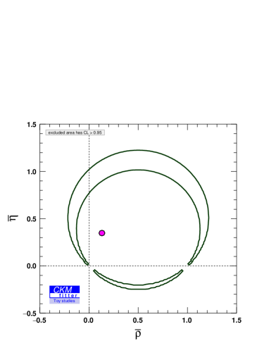
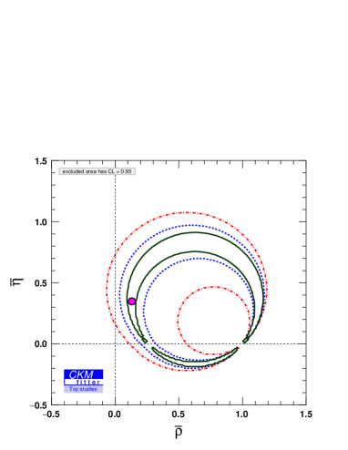
Figure 1: Constraints in the $\bar{\rho}-\bar{\eta}$ plane from the amplitude ratio $R^{0}$ method, using the arbitrary but realistic numerical values for the input parameters, detailed in the text. In the top panel, the $P_{\rm EW}$ hadronic parameter is set to zero. In the bottom panel, the $P_{\rm EW}$ hadronic parameter is set to its true generation value with different theoretical errors on $R$ and $r_{VP}$ parameters (defined in Eq. (39)), either zero (green solid-line contour), 10% and 5% (blue dashed-line contour), and 10% and 30% (red solid-dashed-line contour). The parameters $\bar{\rho}$ and $\bar{\eta}$ are fixed to their current values from the global CKM fit Charles:2004jd ; Charles:2015gya ; CKMfitterwebsite , indicated by the magenta point.

This simple illustration with our reference scenario shows that the CPS/GPSZ method is limited both in robustness and accuracy due to the assumption on a negligible $P_{\rm EW}$: a small non-vanishing value breaks the relation between the phase of $R^{0}$ and the CKM angle $\alpha$, and therefore, even a small uncertainty on the $P_{\rm EW}$ value would translate into large biases on the CKM constraints. It shows that this method would require a very accurate understanding of hadronic amplitudes in order to extract a meaningful constraint on the unitarity triangle, and the presence of non-vanishing electroweak penguins dilutes the potential of this method significantly.

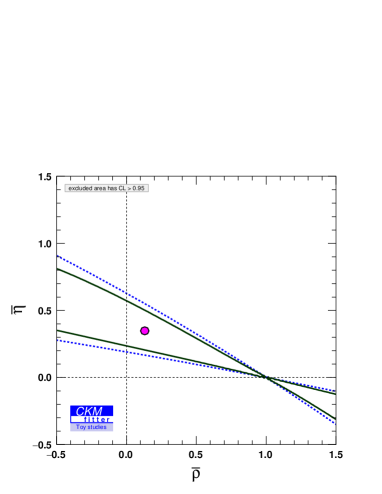
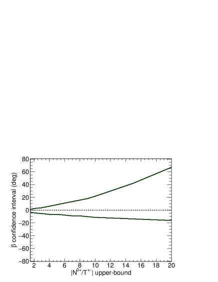
Figure 2: Top: constraints in the $\bar{\rho}-\bar{\eta}$ plane from the annihilation/exchange method, using the arbitrary but realistic numerical values for the input parameters detailed in the text. The green solid-line contour is the constraint obtained by fixing the $N^{0+}$ hadronic parameter to its generation value; the blue dotted-line contour is the constraint obtained by setting an upper bound on the $\left|N^{0+}/T^{+-}\right|$ ratio at twice its generation value. The parameters $\bar{\rho}$ and $\bar{\eta}$ are fixed to their current values from the global CKM fit Charles:2004jd ; Charles:2015gya ; CKMfitterwebsite , indicated by the magenta point. Bottom: size of the $\beta-\beta_{\rm gen}$ 68% confidence interval vs the upper-bound on $|N^{0+}/T^{+-}|$ in units of its generation value.

IV.2 Setting bounds on annihilation/exchange contributions

As discussed in the previous paragraphs, the penguin contributions for $B\rightarrow K^{*}\pi$ decays are strongly CKM-enhanced, impacting the CPS/GPSZ method based on neglecting a penguin amplitude $P_{\rm EW}$. This method exhibits a strong sensitivity to small changes or uncertainties in values assigned to the electroweak penguin contribution. An alternative and safer approach consists in constraining a tree amplitude, with a CKM-suppressed contribution. Among the various hadronic amplitudes introduced, it seems appropriate to choose the annihilation amplitude $N^{0+}$, which is expected to be smaller than $T^{+-}$, and which could even be smaller than the colour-suppressed $T^{00}_{\rm C}$. Unfortunately, no direct, clean constraints on $N^{0+}$ can be extracted from data and from the theoretical point of view, $N^{0+}$ is dominated by incalculable non-factorisable contributions in QCD factorisation Beneke:1999br ; Beneke:2000ry ; Beneke:2003zv ; Beneke:2006hg . On the other hand, indirect upper bounds on $N^{0+}$ may be inferred from either the $B^{+}\to K^{*0}\pi^{+}$ decay rate or from the $U$-spin related mode $B^{+}\to K^{*0}K^{+}$.

This method, like the previous one, hinges on a specific assumption on hadronic amplitudes. Fixing $N^{0+}$ breaks the reparametrisation invariance in Sec. III, and thus provides a way of measuring weak phases. We can compare the two approaches by using the same reference scenario as in Sec. IV.1, i.e., the values gathered in Tab. 11. We have an annihilation parameter $N^{0+}$ with a magnitude $18$ times smaller than the tree parameter $T^{+-}$, and a phase fixed at $108^{\circ}$. All $B\rightarrow K^{*}\pi$ physical observables are used as inputs. This time, all hadronic parameters are free to vary in the fits, except for the annihilation/exchange parameter $N^{0+}$, which is subject to two different hypotheses: either its value is fixed to its generation value, or the ratio $\left|N^{0+}/T^{+-}\right|$ is constrained in a range (up to twice its generation value).

The resulting constraints on the $\bar{\rho}-\bar{\eta}$ are shown on the upper plot of Fig. 2. We stress that in this fit, the value of $N^{0+}$ is bound, but the other amplitudes (including $P_{\rm EW}$) are left free to vary. Using a loose bound on $\left|N^{0+}/T^{+-}\right|$ yields a less tight constraint, but in contrast with the CPS/GPSZ method, the CKM generation value is here included. One may notice that the resulting constraint is similar to the one corresponding to the CKM angle $\beta$. This can be understood in the following way. Let us assume that we neglect the contribution from $N^{0+}$. We obtain the following amplitude to be considered

$$A^{\prime}=A^{0+}=V_{ts}V_{tb}^{*}(-P^{+-}+P_{\rm EW}^{\rm C}),$$ (41)

and then, together with its $CP$-conjugate amplitude $\bar{A}^{\prime}$, a convention-independent amplitude ratio $R^{\prime}$ can be defined as

$$R^{\prime}=\frac{q}{p}\frac{\bar{A}^{\prime}}{A}=e^{-2i\beta}\,,$$ (42)

in agreement with the convention used to fix the phase of the $B$-meson state. This justifies the $\beta$-like shape of the constraint obtained when fixing the value of the annihilation parameter. The presence of the oscillation phase $q/p$ here, starting from a decay of a charged $B$, may seem surprising. However, one should keep in mind that the measurement of $B^{+}\to K^{*0}\pi^{+}$ and its $CP$-conjugate amplitude are not sufficient to determine the relative phase between $A^{\prime}$ and $\bar{A}^{\prime}$: this requires one to reconstruct the whole quadrilateral equation Eq. (23), where the phases are provided by interferences between mixing and decay amplitudes in $B_{0}$ and $\bar{B}_{0}$ decays. In other words, the phase observables obtained from the Dalitz plot are always of the form Eq. (4)-(5): their combination can only lead to a ratio of $CP$-conjugate amplitudes multiplied by the oscillation parameter $q/p$.

The lower plot of Fig. 2 describes how the constraint on $\beta$ loosens around its true value when the range allowed for $\left|N^{0+}/T^{+-}\right|$ is increased compared to its initial value ($0.143$). We see that the method is stable and keeps on including the true value for $\beta$ even in the case of a mild constraint on $\left|N^{0+}/T^{+-}\right|$.

V Constraints on hadronic parameters using current data

As already anticipated in Sec. III, a second strategy to exploit the data consists in assuming that the CKM matrix is already well determined from the CKM global fit Charles:2004jd ; Charles:2015gya ; CKMfitterwebsite . The measurements of $B\rightarrow K^{\star}\pi$ observables (isobar parameters) can then be used to extract constraints on the hadronic parameters in Eq. (28).

V.1 Experimental inputs

For this study, the complete set of available results from the BABAR and Belle experiments is used. The level of detail for the publicly available results varies according to the decay mode in consideration. In most cases, at least one amplitude DP analysis of $B^{0}$ and $B^{+}$ decays is public Amhis:2016xyh , and at least one input from each physical observable is available. In addition, the conventions used in the various DP analyses are usually different. Ideally, one would like to have access to the complete covariance matrix, including statistical and systematic uncertainties, for all isobar parameters, as done for instance in Ref. Aubert:2009me . Since such information is not always available, the published results are used in order to derive ad-hoc approximate covariance matrices, implementing all the available information (central values, total uncertainties, correlations among parameters). The inputs for this study are the following:

• Two three-dimensional covariance matrices, cf. Eq. (10), from the BABAR time-dependent DP analysis of $B^{0}\rightarrow K^{0}_{S}\pi^{+}\pi^{-}$ in Ref. Aubert:2009me , and two three-dimensional covariance matrices from the Belle time-dependent DP analysis of $B^{0}\rightarrow K^{0}_{S}\pi^{+}\pi^{-}$ in Ref. Dalseno:2008wwa . Both the BABAR and Belle analyses found two quasi-degenerate solutions each, with very similar goodness-of-fit merits. The combination of these solutions is described in App. A.3, and is taken as input for this study.

• A five-dimensional covariance matrix, cf. Eq. (11), from the BABAR $B^{0}\rightarrow K^{+}\pi^{-}\pi^{0}$ DP analysis BABAR:2011ae .

• A two-dimensional covariance matrix, cf. Eq. (16), from the BABAR $B^{+}\rightarrow K^{+}\pi^{+}\pi^{-}$ DP analysis Aubert:2008bj , and a two-dimensional covariance matrix from the Belle $B^{+}\rightarrow K^{+}\pi^{+}\pi^{-}$ DP analysis Garmash:2006bj .

• A simplified uncorrelated four-dimensional input, cf. Eq. (17), from the BABAR $B^{+}\rightarrow K^{0}_{S}\pi^{+}\pi^{0}$ preliminary DP analysis Lees:2015uun .

Besides the inputs described previously, there are other experimental measurements on different three-body final states performed in the quasi-two-body approach, which provide measurements of branching ratios and $CP$ asymmetries only. Such is the case of the BABAR result on the $B^{+}\to K^{+}\pi^{0}\pi^{0}$ final state Lees:2011aaa , where the branching ratio and the $CP$ asymmetry of the $B^{+}\to K^{*}(892)^{+}\pi^{0}$ contribution are measured. In this study, these two measurements are treated as uncorrelated, and they are combined with the inputs from the DP analyses mentioned previously.

These sets of experimental central values and covariance matrices are described in App. A, where the combinations of the results from BABAR and Belle are also described.

Finally, we notice that the time-dependent asymmetry in $B\to K_{S}\pi^{0}\pi^{0}$ has been measured Abe:2007xd ; Aubert:2007ub . As these are global analyses integrated over the whole DP, we cannot take these measurements into account. In principle a time-dependent isobar analysis of the $K_{S}\pi^{0}\pi^{0}$ DP could be performed and it could bring some independent information on $B\to K^{*0}\pi^{0}$ intermediate amplitudes. Since this more challenging analysis has not been done yet, we will not consider this channel for the time being.

V.2 Selected results for $CP$ asymmetries and hadronic amplitudes

Using the experimental inputs described in Sec. V.1, a fit to the complete set of hadronic parameters is performed. We discuss the fit results focusing on three aspects: the most significant direct $CP$ asymmetries, the significance of electroweak penguins, and the relative hierarchies of hadronic contributions to the tree amplitudes. As will be seen in the following, the fit results can be interpreted in terms of two sets of local minima, out of which one yields constraints on the hadronic parameters in better agreement with the expectations from CPS/GPSZ, the measured direct $CP$ asymmetries and the expected relative hierarchies of hadronic contributions.

V.2.1 Direct $CP$ violation in $B^{0}\rightarrow K^{\star+}\pi^{-}$

The $B^{0}\rightarrow K^{\star+}\pi^{-}$ amplitude can be accessed both in the $B^{0}\rightarrow K^{0}_{\rm S}\pi^{+}\pi^{-}$ and $B^{0}\rightarrow K^{+}\pi^{-}\pi^{0}$ Dalitz-plot analyses. The direct $CP$ asymmetry $A_{\rm CP}(B^{0}\rightarrow K^{\star+}\pi^{-})$ has been measured by BABAR in both modes BABAR:2011ae ; Aubert:2009me and by Belle in the $B^{0}\rightarrow K^{0}_{\rm S}\pi^{+}\pi^{-}$ mode Dalseno:2008wwa . All three measurements yield a negative value: incidentally, this matches also the sign of the two-body $B^{0}\rightarrow K^{+}\pi^{-}$ $CP$ asymmetry, for which direct $CP$ violation is clearly established.

Using the amplitude DP analysis results from these three measurements as inputs, the combined constraint on $A_{\rm CP}(B^{0}\rightarrow K^{\star+}\pi^{-})$ is shown in Fig. 3. The combined value is 3.0 $\sigma$ away from zero, and the 68% confidence interval on this $CP$ asymmetry is $0.21\pm 0.07$ approximately. This result is to be compared with the $0.23\pm 0.06$ value provided by HFLAV Amhis:2016xyh . The difference is likely to come from the fact that HFLAV performs an average of the $CP$ asymmetries extracted from individual experiments, while this analysis uses isobar values as inputs which are averaged over the various experiments before being translated into values for the $CP$ parameters: since the relationships between these two sets of quantities are non-linear, the two steps (averaging over experiments and translating from one type of observables to another) yield the same central values only in the case of very small uncertainties. In the current situation, where sizeable uncertainties affect the determinations from individual experiments, it is not surprising that minor discrepancies arise between our approach and the HFLAV result.

As can be readily seen from Eq. (22), a non-vanishing asymmetry in this mode requires a strong phase difference between the tree $T^{+-}$ and penguin $P^{+-}$ hadronic parameters that is strictly different from zero. Fig. 4 shows the two-dimensional constraint on the modulus and phase of the $P^{+-}/T^{+-}$ ratio. Two solutions with very similar $\chi^{2}$ are found, both incompatible with a vanishing phase difference. The first solution corresponds to a small (but non-vanishing) positive strong phase, with similar $\left|V_{ts}V_{tb}^{\star}P^{+-}\right|$ and $\left|V_{us}V_{ub}^{\star}T^{+-}\right|$ contributions to the total decay amplitude, and is called Solution I in the following. The other solution, denoted Solution II, corresponds to a larger, negative, strong phase, with a significantly larger penguin contribution. We notice that Solution I is closer to usual theoretical expectations concerning the relative size of penguin and tree contributions.

Let us stress that the presence of two solutions for $P^{+-}/T^{+-}$ is not related to the presence of ambiguities in the individual BABAR and Belle measurements for $B^{+}\to K^{+}\pi^{+}\pi^{-}$ and $B^{0}\to K^{0}_{S}\pi^{+}\pi^{-}$, since we have performed their combinations in order to select a single solution for each process. Therefore, the presence of two solutions in Fig. 4 is a global feature of our non-linear fit, arising from the overall structure of the current combined measurements (central values and uncertainties) that we use as inputs.

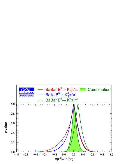
Figure 3: Constraint on the direct $CP$ asymmetry parameter $C(B^{0}\rightarrow K^{\star+}\pi^{-})=-A_{\rm CP}(B^{0}\rightarrow K^{\star+}\pi^{-})$ from BABAR data on $B^{0}\to K^{0}_{S}\pi^{+}\pi^{-}$ (red curve), Belle data on $B^{0}\to K^{0}_{S}\pi^{+}\pi^{-}$ (blue curve), BABAR data on $B^{0}\to K^{+}\pi^{-}\pi^{0}$ (green curve) and the combination of all these measurements (green shaded curve). The constraints are obtained using the observables described in the text.

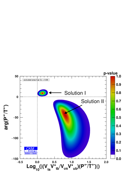
Figure 4: Two-dimensional constraint on the modulus and phase of the $P^{+-}/T^{+-}$ ratio. For convenience, the modulus is multiplied by the ratio of CKM factors appearing in the tree and penguin contributions to the $B^{0}\rightarrow K^{\star+}\pi^{-}$ decay amplitude.

V.2.2 Direct $CP$ violation in $B^{+}\rightarrow K^{\star+}\pi^{0}$

The $B^{+}\rightarrow K^{\star+}\pi^{0}$ amplitude can be accessed in a $B^{+}\rightarrow K^{0}_{\rm S}\pi^{+}\pi^{0}$ Dalitz-plot analysis, for which only a preliminary result from BABAR is available Lees:2015uun . A large, negative $CP$ asymmetry $A_{\rm CP}(B^{+}\rightarrow K^{\star+}\pi^{0})=-0.52\pm 0.14\pm 0.04^{+0.04}_{-0.02}$ is reported there with a 3.4 $\sigma$ significance. This $CP$ asymmetry has also been measured by BABAR through a quasi-two-body analysis of the $B^{+}\rightarrow K^{+}\pi^{0}\pi^{0}$ final state Lees:2011aaa , obtaining $A_{\rm CP}(B^{+}\rightarrow K^{\star+}\pi^{0})=-0.06\pm 0.24\pm 0.04$. The combination of these two measurement yields $A_{\rm CP}(B^{+}\rightarrow K^{\star+}\pi^{0})=-0.39\pm 0.12\pm 0.03$, with a 3.2 $\sigma$ significance.

In contrast with the $B^{0}\rightarrow K^{\star+}\pi^{-}$ case, in the canonical parametrisation Eq. (28), the decay amplitude for $B^{+}\rightarrow K^{\star+}\pi^{0}$ includes several hadronic contributions both to the total tree and penguin terms, namely

$$\sqrt{2}A^{+0} = V_{us}V_{ub}^{*}T^{+0}+V_{ts}V_{tb}^{*}P^{+0}$$

$$= V_{us}V_{ub}^{*}(T^{+-}+T_{\rm C}^{00}-N^{0+})$$

$$+V_{ts}V_{tb}^{*}(P^{+-}+P_{\rm EW}-P_{\rm EW}^{\rm C})\ ,$$

and therefore no straightforward constraint on a single pair of hadronic parameters can be extracted, as several degenerate combinations can reproduce the observed value of the $CP$ asymmetry $A_{\rm CP}(B^{+}\rightarrow K^{\star+}\pi^{0})$. This is illustrated in Fig. 6, where six different local minima are found in the fit, all with similar $\chi^{2}$ values. The three minima with positive strong phases correspond to Solution I, while the three minima with negative strong phases correspond to Solution II. The relative size of the total tree and penguin contributions is bound within a relatively narrow range: we get $|P^{+0}/T^{+0}|\in(0.018,0.126)$ at $68\%$ C.L.

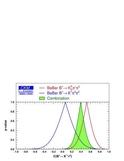
Figure 5: Constraint on the direct $CP$ asymmetry parameter $C(B^{+}\rightarrow K^{\star+}\pi^{0})=-A_{\rm CP}(B^{+}\rightarrow K^{\star+}\pi^{0})$ from BABAR data on $B^{+}\to K^{0}_{S}\pi^{+}\pi^{0}$ (red curve), BABAR data on $B^{+}\to K^{+}\pi^{0}\pi^{0}$ (blue curve) and the combination (green shaded curve). The constraints are obtained using the observables described in the text.

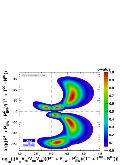
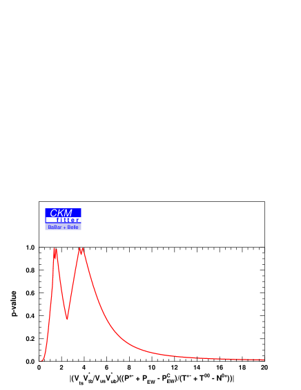
Figure 6: Top: two-dimensional constraint on the modulus and phase of the $(P^{+-}+P_{\rm EW}-P_{\rm EW}^{\rm C})/(T^{+-}+T_{\rm C}^{00}-N^{0+})$ ratio. For convenience, the modulus is multiplied by the ratio of CKM factors appearing in the tree and penguin contributions to the $B^{+}\rightarrow K^{\star+}\pi^{0}$ decay amplitude. Bottom: one-dimensional constraint on the modulus of the $(P^{+-}+P_{\rm EW}-P_{\rm EW}^{\rm C})/(T^{+-}+T_{\rm C}^{00}-N^{0+})$ ratio.

V.2.3 Hierarchy among penguins: electroweak penguins

In Sec. IV.1, we described the CPS/GPSZ method designed to extract weak phases from $B\to\pi K$ assuming some control on the size of the electroweak penguin. According to this method, the electroweak penguin is expected to yield a small contribution to the decay amplitudes, with no significant phase difference. We are actually in a position to test this expectation by fitting the hadronic parameters using the BABAR and Belle data as inputs. Fig. 7 shows the two-dimensional constraint on $r_{VP}$, in other words, the ratio $P_{\rm EW}/T_{3/2}$ ratio, showing two local minima. The CPS/GPSZ prediction is also indicated in this figure. In Fig. 8, we provide the regions allowed for $|r_{VP}|$ and the modulus of the ratio $|P^{+-}/T^{+-}|$, exhibiting two favoured values, the smaller one being associated with Solution I and the larger one with Solution II. The latter one corresponds to a significantly large electroweak penguin amplitude and it is clearly incompatible with the CPS/GPSZ prediction by more than one order of magnitude. A better agreement, yet still marginal, is found for the smaller minimum that corresponds to Solution I: the central value for the ratio is about a factor of three larger than CPS/GPSZ, and a small, positive phase is preferred. For this minimum, an inflation of the uncertainty on $\left|r_{\rm VP}\right|$ up to $30\%$ would be needed to ensure proper agreement. In any case, it is clear that the data prefers a larger value of $|r_{\rm VP}|$ than the estimates originally proposed.

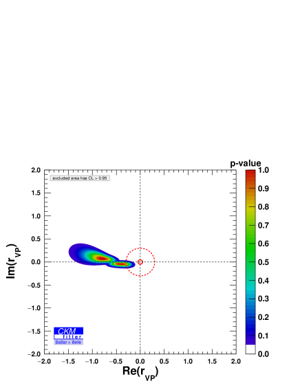
Figure 7: Two-dimensional constraint on real and imaginary parts on the $r_{VP}$ parameter defined in Eq. (39). The area encircled with the solid (dashed) red line corresponds to the CPS/GPSZ prediction, with a $5\%$ ($30\%$) uncertainty on the $r_{\rm VP}$ parameter.

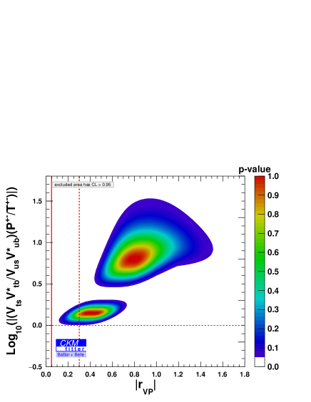
Figure 8: Two-dimensional constraint on $|r_{VP}|$ defined in Eq. (39) and ${\rm Log}_{10}\left(|P^{+-}/T^{+-}|\right)$. The vertical solid (dashed) red line corresponds to the CPS/GPSZ prediction, with a $5\%$ ($30\%$) uncertainty.

Moreover, the contribution from the electroweak penguin is found to be about twice larger than the main penguin contribution $P^{+-}$. This is illustrated in Fig. 9, where only one narrow solution is found in the $P_{\rm EW}/P^{+-}$ plane, as both solutions I and II provide essentially the same constraint. The relative phase between these two parameters is bound to the interval $(-25,+10)^{\circ}$ at $95\%$ C.L. Additional tests allow us to demonstrate that this strong constraint on the relative $P_{\rm EW}/P^{+-}$ penguin contributions is predominantly driven by the $\varphi^{00,+-}$ phase differences measured in the BABAR Dalitz-plot analysis of $B^{0}\rightarrow K^{+}\pi^{+}\pi^{0}$ decays. The strong constraint on the $P_{\rm EW}/P^{+-}$ ratio is turned into a mild upper bound when removing the $\varphi^{00,+-}$ phase differences from the experimental inputs. The addition of these two observables as fit inputs increases the minimal $\chi^{2}$ by 7.7 units, which corresponds to a 2.6 $\sigma$ discrepancy. Since the latter is driven by a measurement from a single experiment, additional experimental results are needed to confirm such a large value for the electroweak penguin parameter.

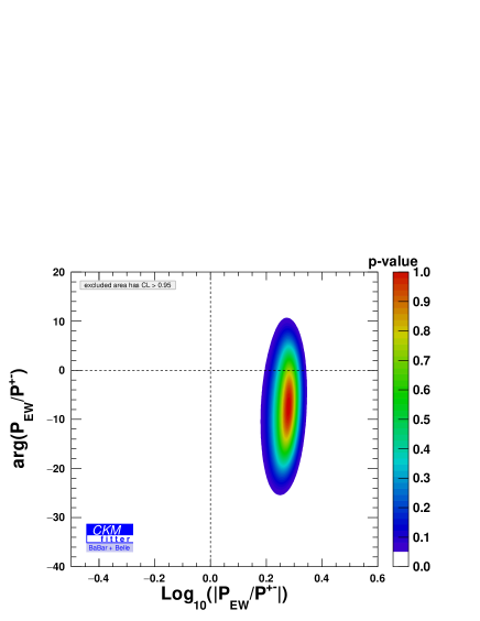
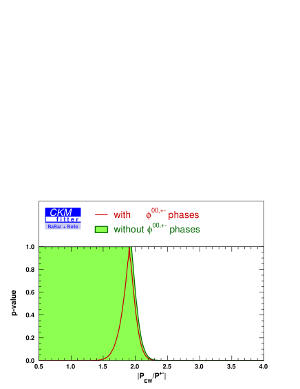
Figure 9: Top: two-dimensional constraint on the modulus and phase of the complex $P_{\rm EW}/P^{+-}$ ratio. Bottom: constraint on the $\left|P_{\rm EW}/P^{+-}\right|$ ratio, using the complete set of experimental inputs (red curve), and removing the BABAR measurement of the $\varphi^{00,+-}$ phases from the $B^{0}\rightarrow K^{+}\pi^{+}\pi^{0}$ Dalitz-plot analysis (green shaded curve).

In view of colour suppression, the electroweak penguin $P_{\rm EW}^{\rm C}$ is expected to yield a smaller contribution than $P_{\rm EW}$ to the decay amplitudes. This hypothesis is tested in Fig. 10, which shows that current data favours a similar size for the two contributions, and a small relative phase (up to $40^{\circ}$) between the colour-allowed and the colour-suppressed electroweak penguins. Both Solutions I and II show the same structure with four different local minima.

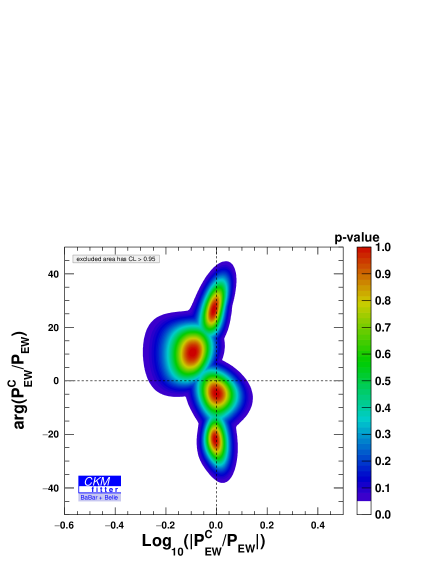
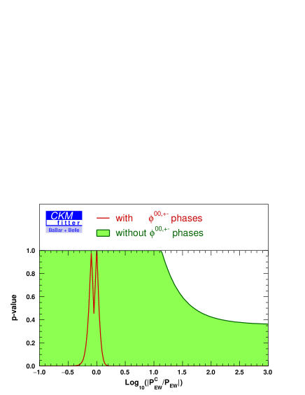
Figure 10: Top: two-dimensional constraint on the modulus and phase of the $P_{\rm EW}^{\rm C}/P_{\rm EW}$ ratio. Bottom: one-dimensional constraint on ${\rm Log}_{10}\left(\left|P_{\rm EW}^{\rm C}/P_{\rm EW}\right|\right)$, using the complete set of experimental inputs (red curve), and removing the BABAR measurement of the $\varphi^{00,+-}$ phases from the $B^{0}\rightarrow K^{+}\pi^{+}\pi^{0}$ Dalitz-plot analysis (green shaded curve).

V.2.4 Hierarchy among tree amplitudes: colour suppression and annihilation

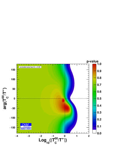
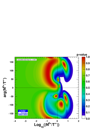
Figure 11: Two-dimensional constraint on the modulus and phase of the $T^{00}_{\rm C}/T^{+-}$ (top) and $N^{0+}/T^{+-}$ (bottom) ratios.

As already discussed, the hadronic parameter $T^{00}_{\rm C}$ is expected to be suppressed with respect to the main tree parameter $T^{+-}$. Also, the annihilation topology is expected to provide negligible contributions to the decay amplitudes. These expectations can be compared with the extraction of these hadronic parameters from data in Fig. 11.

For colour suppression, the current data provides no constraint on the relative phase between the $T^{00}_{\rm C}$ and $T^{+-}$ tree parameters, and only a mild upper bound on the modulus can be inferred; the tighter constraint is provided by Solution I that excludes values of $|T^{00}_{\rm C}/T^{+-}|$ larger than $1.6$ at $95\%$ C.L. The constraint from Solution II is more than one order of magnitude looser.

Similarly, for annihilation, Solution I provides slightly tighter constraints on its contribution to the total tree amplitude with the bound $|N^{0+}/T^{+-}|<2.5$ at $95\%$ C.L., while the bound from Solution II is much looser.

V.3 Comparison with theoretical expectations

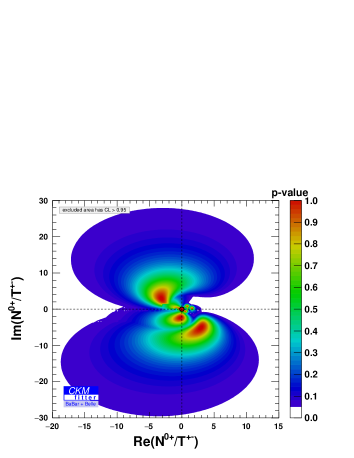
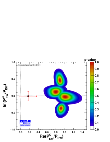
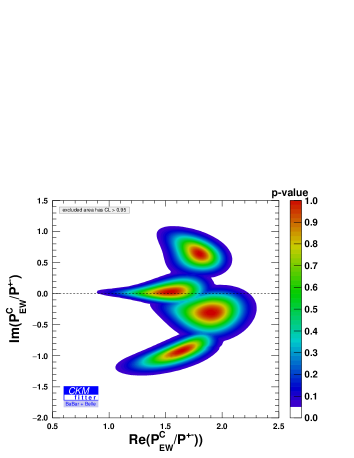
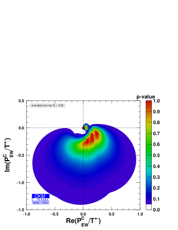
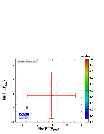
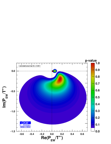
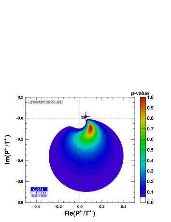
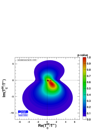
Figure 12: Two-dimensional constraints on the real and imaginary parts of hadronic ratios, respectively from left to right and from top to bottom: $N^{0+}/T^{+-}$, $P_{\rm EW}^{\rm C}/P_{\rm EW}$, $P_{\rm EW}^{\rm C}/P^{+-}$, $P_{\rm EW}^{\rm C}/T^{+-}$, $P^{+-}/P_{\rm EW}$, $P_{\rm EW}/T^{+-}$, $P^{+-}/T^{+-}$ and $T^{00}_{\rm C}/T^{+-}$. The red crosses and dots indicate our predictions based on QCD factorisation. No prediction is given for the ratio ${P_{\rm EW}^{\rm C}}/{P^{+-}}$ due to numerical instabilities (see text).

Quantity	Fit result	QCDF
$\displaystyle{\mathcal{R}e}\frac{N^{0+}}{T^{+-}}$	$(-5.31,4.73)$	$0.011\pm 0.027$
$\displaystyle{\mathcal{I}m}\frac{N^{0+}}{T^{+-}}$	$(-9.59,7.73)$	$0.003\pm 0.028$
$\displaystyle{\mathcal{R}e}\frac{P_{\rm EW}^{\rm C}}{P_{\rm EW}}$	$(0.69,1.14)$	$0.17\pm 0.19$
$\displaystyle{\mathcal{I}m}\frac{P_{\rm EW}^{\rm C}}{P_{\rm EW}}$	$(-0.48,-0.28)~{}\cup~{}(-0.13,0.22)~{}\cup$	$-0.08\pm 0.14$
	$(0.34,0.60)$
$\displaystyle{\mathcal{R}e}\frac{P_{\rm EW}^{\rm C}}{P^{+-}}$	$(1.29,2.08)$	$-$
$\displaystyle{\mathcal{I}m}\frac{P_{\rm EW}^{\rm C}}{P^{+-}}$	$(-1.09,-0.75)~{}\cup~{}(-0.51,-0.10)~{}\cup$	$-$
	$(-0.08,0.16)~{}\cup~{}(0.47,0.83)$
$\displaystyle{\mathcal{R}e}\frac{P_{\rm EW}^{\rm C}}{T^{+-}}$	$(-0.12,0.34)$	$0.0027\pm 0.0031$
$\displaystyle{\mathcal{I}m}\frac{P_{\rm EW}^{\rm C}}{T^{+-}}$	$(-0.42,0.05)$	$-0.0015^{+0.0024}_{-0.0025}$
$\displaystyle{\mathcal{R}e}\frac{P^{+-}}{P_{\rm EW}}$	$(0.49,0.56)$	$3.9^{+3.2}_{-3.3}$
$\displaystyle{\mathcal{I}m}\frac{P^{+-}}{P_{\rm EW}}$	$(-0.03,0.16)$	$1.8\pm 3.3$
$\displaystyle{\mathcal{R}e}\frac{P_{\rm EW}}{T^{+-}}$	$(0.0,0.25)$	$0.0154^{+0.0059}_{-0.0060}$
$\displaystyle{\mathcal{I}m}\frac{P_{\rm EW}}{T^{+-}}$	$(-0.40,-0.09)~{}\cup~{}(-0.02,0.02)$	$-0.0014^{+0.0023}_{-0.0022}$
$\displaystyle{\mathcal{R}e}\frac{P^{+-}}{T^{+-}}$	$(0.023,0.140)$	$0.053\pm 0.039$
$\displaystyle{\mathcal{I}m}\frac{P^{+-}}{T^{+-}}$	$(-0.20,-0.04)~{}\cup~{}(0.0,0.01)$	$0.016\pm 0.044$
$\displaystyle{\mathcal{R}e}\frac{T^{00}_{\rm C}}{T^{+-}}$	$(-0.26,2.24)$	$0.13\pm 0.17$
$\displaystyle{\mathcal{I}m}\frac{T^{00}_{\rm C}}{T^{+-}}$	$(-3.28,0.74)$	$-0.11\pm 0.15$

Table 1: $68\%$ confidence intervals for the real and imaginary parts of hadronic ratios according to our fit and the corresponding predictions in our implementation of QCD factorisation (QCDF). No prediction is given for the ratio ${P_{\rm EW}^{\rm C}}/{P^{+-}}$ due to numerical instabilities (see text).

We have extracted the values of the hadronic amplitudes from the data currently available. It may prove interesting to compare these results with theoretical expectations. For this exercise, we use QCD factorisation Beneke:1999br ; Beneke:2000ry ; Beneke:2003zv ; Beneke:2006hg as a benchmark point, keeping in mind that other approaches (discussed in the introduction) are available. In order to keep the comparison simple and meaningful, we consider the real and imaginary part of several ratios of hadronic amplitudes.

We obtain our theoretical values in the following way. We follow Ref. Beneke:2003zv for the expressions within QCD factorisation, and we use the same model for the power-suppressed and infrared-divergent contributions coming from hard scattering and weak annihilation: these contributions are formally $1/m_{b}$-suppressed but numerically non negligible, and play a crucial role in some of the amplitudes. On the other hand, we update the hadronic parameters in order to take into account more recent determinations of these quantities, see App. B. We use the Rfit scheme to handle theoretical uncertainties Charles:2004jd ; Charles:2015gya ; CKMfitterwebsite ; Charles:2016qtt (in particular for the hadronic parameters and the $1/m_{b}$ power-suppressed contributions), and we compute only ratios of hadronic amplitudes using QCD factorisation. We stress that we provide the estimates within QCD factorisation simply to compare the results of our experimental fit for the hadronic amplitudes with typical theoretical expectations concerning the same quantities. In particular we neglect Next-Next-to-Leading Order corrections that have been partially computed in Refs. BHWS ; Bell:2007tv ; Bell:2009nk ; Beneke:2009ek ; Bell:2015koa , and we do not attempt to perform a fully combined fit of the theoretical predictions with the experimental data, as the large uncertainties would make the interpretation difficult.

Our results for the ratios of hadronic amplitudes are shown in Fig. 12 and in Tab. 1. We notice that for most of the ratios, a good agreement is found. The global fit to the experimental data has often much larger uncertainties than theoretical predictions: with better data in the future, we may be able to perform very non trivial tests of the non-leptonic dynamics and the isobar approximation. The situation for $P_{\rm EW}^{\rm C}/P_{\rm EW}$ is slightly different, since the two determinations (experiment and theory) exhibit similar uncertainties and disagree with each other, providing an interesting test for QCD factorisation, which however goes beyond the scope of this study.

There are two cases where the theoretical output from QCD factorisation is significantly less precise than the constraints from the combined fit. For $P_{\rm EW}^{C}/P^{+-}$, both numerator and denominator can be (independently) very small in QCD factorisation, and numerical instabilities in this ratio prevent us from having a precise prediction. For $P^{+-}/P_{\rm EW}$, the impressively accurate experimental determination, as discussed in Sec. V.2.3, is predominantly driven by the $\varphi^{00,+-}$ phase differences measured in the BABAR Dalitz-plot analysis of $B^{0}\rightarrow K^{+}\pi^{+}\pi^{0}$ decays. Removing this input yields a much milder constraint on $P^{+-}/P_{\rm EW}$. On the other hand in QCD factorisation, the formally leading contributions to the $P^{+-}$ penguin amplitude are somewhat numerically suppressed, and compete with the model estimate of power corrections: due to the Rfit treatment used, the two contributions can either compensate each other almost exactly or add up coherently, leading to a $\sim\pm 100\%$ relative uncertainty, which is only in marginal agreement with the fit output. Thus we conclude that the $P^{+-}/P_{\rm EW}$ ratio is both particularly sensitive to the power corrections to QCD factorisation and experimentally well constrained, so that it can be used to provide an insight on non factorisable contributions, provided one assumes negligible effects from New Physics.

VI Prospects for LHCb and Belle II

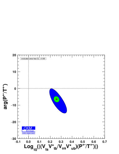
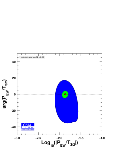
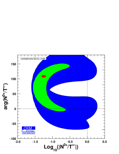
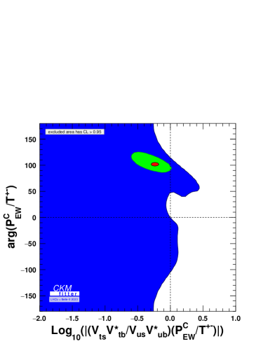
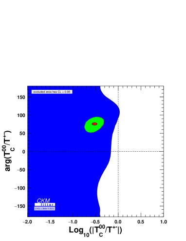
Figure 13: The expected two-dimensional constraints on the moduli and phases of various ratios of hadronic parameters, using inputs from the first-step of the prospective study, based on results from the $B$-factories and expected sensitivities for LHCb Run1+Run2 (blue area); and using inputs from the second-step of the prospective study, based on the complete set of results from LHCb and Belle II (green area). The red spots in the figures represent the generation values obtained from Tab. 11. From top to bottom and left to right, the hadronic ratios are: $P^{+-}/T^{+-}$, $P_{\rm EW}/T_{3/2}$, $N^{0+}/T^{+-}$, $P_{\rm EW}^{\rm C}/T^{+-}$, and $T^{00}_{\rm C}/T^{+-}$, respectively.

In this section, we study the impact of improved measurements of $K\pi\pi$ modes from the LHCb and Belle II experiments. During the first run of the LHC, the LHCb experiment has collected large datasets of B-hadron decays, including charmless $B^{0},B^{+},B_{s}$ meson decays into tree-body modes. LHCb is currently collecting additional data in Run-2. In particular, due to the excellent performances of the LHCb detector for identifying charged long-lived mesons, the experiment has the potential for producing the most accurate charmless three-body results in the $B^{+}\rightarrow K^{+}\pi^{-}\pi^{+}$ mode, owing to high-purity event samples much larger than the ones collected by BABAR and Belle. Using $3.0\ {\rm fb}^{-1}$ of data recorded during the LHC Run 1, first results on this mode are already available Aaij:2014iva , and a complete amplitude analysis is expected to be produced in the short-term future. For the $B^{0}\rightarrow K^{0}_{S}\pi^{+}\pi^{-}$ mode, the event-collection efficiency is challenged by the combined requirements on reconstructing the $K^{0}_{S}\rightarrow\pi^{+}\pi^{-}$ decay and tagging the $B$ meson flavour, but nonetheless the $B^{0}\rightarrow K^{0}_{S}\pi^{+}\pi^{-}$ data samples collected by LHCb are already larger than the ones from BABAR and Belle. As it is more difficult to anticipate the reach of LHCb Dalitz-plot analyses for modes including $\pi^{0}$ mesons in the final state, the $B^{0}\rightarrow K^{+}\pi^{+}\pi^{0}$, $B^{+}\rightarrow K^{0}_{S}\pi^{+}\pi^{0}$ $B^{+}\rightarrow K^{+}\pi^{0}\pi^{0}$ and $B^{0}\rightarrow K_{S}^{0}\pi^{0}\pi^{0}$ channels are not considered here. In addition, LHCb has also the potential for studying $B_{s}$ decay modes, and LHCb can reach $B\to KK\pi$ modes with branching ratios out of reach for $B$-factories.

The Belle II experiment Urquijo:2015qsa , currently in the stages of construction and commissioning, will operate in an experimental environment very similar to the one of the BABAR and Belle experiments. Therefore Belle II has the potential for studying all modes accessed by the $B$-factories, with expected sensitivities that should scale in proportion to its expected total luminosity (i.e., $50\ {\rm ab}^{-1}$). In addition, Belle II has the potential for accessing the $B^{+}\rightarrow K^{+}\pi^{0}\pi^{0}$ and $B^{0}\rightarrow K_{S}^{0}\pi^{0}\pi^{0}$ modes (for which the $B$-factories could not produce Dalitz-plot results) but these modes will provide low-accuracy information, redundant with some of the modes considered in this paper: therefore they are not included here.

Since both the LHCb and Belle II have the potential for studying large, high-quality samples of $B^{+}\rightarrow K^{+}\pi^{-}\pi^{+}$, it is realistic to expect that the experiments will be able to extract a consistent, data-driven signal model to be used in all Dalitz-plot analysis, yielding systematic uncertainties significantly decreased with respect to the results from $B$-factories.

Finally for LHCb, since this experiment cannot perform $B$-meson counting as in a $B$-factory environment, the branching fractions need to be normalised with respect to measurements performed at BABAR and Belle, until the advent of Belle II. This prospective study therefore is split into two periods: a first one based on the assumption of new results from LHCb Run1+Run2 only, and a second one using the complete set of LHCb and Belle II results. The corresponding inputs are gathered in App. C. We use the reference scenario described in Tab. 11 for the central values, so that we can guarantee the self-consistency of the inputs and we avoid reducing the uncertainties artificially because of barely compatible measurements (which would occur if we used the central values of the current data and rescaled the uncertainties). The expected uncertainties, obtained from the extrapolations discussed previously, are described in Tab. 12.

The blue area in Fig. 13 illustrates the potential for the first step of our prospective study ($B$-factories and LHCb Run1+Run2). For the input values used in the prospective, the modulus of the $P^{+-}/T^{+-}$ ratio will be constrained with a relative $10\%$ accuracy, and its complex phase will be constrained within $3$ degrees (we discuss 68% C.L. ranges in the following, whereas Fig. 13 shows 95% C.L. regions). Slightly tighter upper bounds on the $|T^{00}_{\rm C}/T^{+-}|$ and $|N^{0+}/T^{+-}|$ ratios may be set, albeit the relative phases of these rations will remain very poorly constrained. Assuming that the electroweak penguin is in agreement with the CPS/GPSZ prediction, its modulus will be constrained within $45\%$ and its phase within $14$ degrees.

The addition of results from the Belle II experiment corresponds to the second step of this prospective study. As illustrated by the green area in Fig. 13, the uncertainties on the modulus and phase of the $P^{+-}/T^{+-}$ ratio will decrease by factors of $1.4$ and $2.5$, respectively. Owing to the addition of precision measurements by Belle II of the $B^{0}\to K^{*0}\pi^{0}$ Dalitz-plot parameters from the amplitude analysis of the $B^{0}\to K^{+}\pi^{-}\pi^{0}$ modes, the $T^{00}_{\rm C}/T^{+-}$ ratio can be constrained within a $22\%$ uncertainty for its modulus, and within $10$ degrees for its phase. Similarly, the uncertainties on the modulus and phase of the $P_{\rm EW}/T_{3/2}$ ratio will decrease by factors $2.7$ and $2.9$, respectively. Concerning the colour-suppressed electroweak penguin, for which only a mild upper bound on its modulus was achievable within the first step of the prospective, can now be measured within a $22\%$ uncertainty for its modulus, and within $8$ degrees for its phase. Finally, the less stringent constraint will be achieved for the annihilation parameter. While its modulus can nevertheless be constrained between 0.3 and 1.5, the phase of this ratio may remain unconstrained in value, with just the sign of the phase being resolved. We add that one can also expect Belle II measurements for $B^{+}\to K^{+}\pi^{0}\pi^{0}$ and $B^{0}\to K_{S}\pi^{0}\pi^{0}$, however with larger uncertainties, so that we have not taken into account these decays.

In total, precise constraints on almost all hadronic parameters in the $B\rightarrow K^{\star}\pi$ system will be achieved using the Dalitz-plot results from the LHCb and Belle II experiments, with a resolution of the current phase ambiguities. These constraints can be compared with various theoretical predictions, proving an important tool for testing models of hadronic contributions to charmless $B$ decays.

VII Conclusion

Non-leptonic B meson decays are very interesting processes both as probes of weak interaction and as tests of our understanding of QCD dynamics. They have been measured extensively at $B$-factories as well as at the LHCb experiment, but this wealth of data has not been fully exploited yet, especially for the pseudoscalar-vector modes which are accessible through Dalitz-Plot analyses of $B\to K\pi\pi$ modes. We have focused on the $B\to K^{*}\pi$ system which exhibits a large set of observables already measured. Isospin analysis allows us to express this decay in terms of CKM parameters and 6 complex hadronic amplitudes, but reparametrisation invariance prevents us from extracting simultaneously information on the weak phases and the hadronic amplitudes needed to describe these decays. We have followed two different approaches to exploit this data: either we extracted information on the CKM phase (after setting a condition on some of the hadronic amplitudes), or we determined of hadronic amplitudes (once we set the CKM parameters to their value from the CKM global fit Charles:2004jd ; Charles:2015gya ; CKMfitterwebsite ).

In the first case, we considered two different strategies. We first reconsidered the CPS/GPSZ strategy proposed in Ref. Ciuchini:2006kv ; Gronau:2006qn , amounting to setting a bound on the electroweak penguin in order to extract an $\alpha$-like constraint. We used a reference scenario inspired by the current data but with consistent central values and much smaller uncertainties in order to probe the robustness of the CPS/GPSZ method: it turns out that the method is easily biased if the bound on the electroweak penguin is not correct, even by a small amount. Unfortunately, this bound is not very precise from the theoretical point of view, which casts some doubt on the potential of this method to constrain $\alpha$. We have then considered a more promising alternative, consisting in setting a bound on the annihilation contribution. We observed that we could obtain an interesting stable $\beta$-like constraint and we discussed its potential to extract confidence intervals according to the accuracy of the bound used for the annihilation contribution.

In a second stage, we discussed how the data constrain the hadronic amplitudes, assuming the values of the CKM parameters. We performed an average of BABAR and Belle data in order to extract constraints on various ratios of hadronic amplitudes, with the issue that some of these data contain several solutions to be combined in order to obtain a single set of inputs for the Dalitz-plot observables. The ratio $P^{+-}/T^{+-}$ is not very well constrained and exhibits two distinct preferred solutions, but it is not large and supports the expect penguin suppression. On the other hand, colour or electroweak suppression does not seem to hold, as illustrated by $|P_{\rm EW}/P^{+-}|$ (around 2), $|P_{\rm EW}^{\rm C}/P_{\rm EW}|$ (around 1) or $|T^{00}_{\rm C}/T^{+-}|$ (mildly favouring values around 1). We however recall that some of these conclusions are very dependent on the BABAR measurement on $\varphi^{00,+-}$ phase differences measured in $B^{0}\to K^{+}\pi^{+}\pi^{0}$: removing this input turns the ranges into mere upper bounds on these ratios of hadronic amplitudes.

For illustration purposes, we compared these results with typical theoretical expectations. We determined the hadronic amplitudes using an updated implementation of QCD factorisation. A good overall agreement between theory and experiment is found for most of the ratios of hadronic amplitudes, even though the experimental determinations remain often less accurate than the theoretical determinations in most instances. Nevertheless, two quantities still feature interesting properties. The ratio $P^{+-}/P_{\rm EW}$ could provide interesting constraints on the models used to describe power-suppressed contributions in QCD factorisation, keeping in mind the (precise) experimental determination of this ratio relies strongly on the $\varphi^{00,+-}$ phases measured by BABAR, as discussed in the previous paragraph. The ratio $P_{\rm EW}^{C}/P_{\rm EW}$ is determined with similar accuracies theoretically and experimentally, but the two determinations are not in good agreement, suggesting that this quantity could also be used to constrain QCD factorisation parameters.

Finally, we performed prospective studies, considering two successive stages based first on LHCb data from Run1 and Run2, then on the additional input from Belle II. Using our reference scenario and extrapolating the uncertainties of the measurements at both stages, we determined the confidence regions for the moduli and phases of the ratios of hadronic amplitudes. The first stage (LHCb only) would correspond to a significant improvement for $P^{+-}/T^{+-}$ and $P_{\rm EW}/T_{3/2}$, whereas the second stage (LHCb+Belle II) would yield tight constraints on $N^{0+}/T^{+-}$, $P_{\rm EW}^{C}/T^{+-}$ and $T^{00}_{\rm C}/T^{+-}$.

Non-leptonic $B$-meson decays remain an important theoretical challenge, and any contender should be able to explain not only the pseudoscalar-pseudoscalar modes but also the pseudoscalar-vector modes. Unfortunately, the current data do not permit such extensive tests, even though they hint at potential discrepancies with theoretical expectations concerning the hierarchies of hadronic amplitudes. However, our study suggests that a more thorough analysis of $B\to K\pi\pi$ Dalitz plots from LHCb and Belle II could allow for a precise determination of the hadronic amplitudes involved in $B\to K^{*}\pi$ decays thanks to the isobar approximation for three-body amplitudes. This will definitely shed some light on the complicated dynamics of weak and strong interaction at work in pseudo-scalar-vector modes, and it will provide important tests of our understanding of non-leptonic $B$-meson decays.

VIII Acknowledgments

We would like to thank all our collaborators from the CKMfitter group for useful discussions, and Reina Camacho Toro for her collaboration on this project at an early stage. This project has received funding from the European Union Horizon 2020 research and innovation programme under the grant agreements No 690575. No 674896 and No. 692194. SDG acknowledges partial support from Contract FPA2014-61478-EXP.

Appendix A Current experimental inputs

The full set real-valued physical observables, derived from the experimental inputs from BABAR and Belle, is described in the following sections. The errors and correlation matrices include both statistical and systematic uncertainties.

$B^{0}\rightarrow K^{0}_{S}\pi^{+}\pi^{-}$	Global min	${\mathcal{R}e}\left[\frac{q}{p}\frac{\overline{A}(K^{*-}\pi^{+})}{A(K^{*+}\pi^{-})}\right]$	${\mathcal{I}m}\left[\frac{q}{p}\frac{\overline{A}(K^{*-}\pi^{+})}{A(K^{*+}\pi^{-})}\right]$	${\mathcal{B}}(K^{*+}\pi^{-})$
${\mathcal{R}e}\left[\frac{q}{p}\frac{\overline{A}(K^{*-}\pi^{+})}{A(K^{*+}\pi^{-})}\right]$	$0.428\pm 0.473$	1.00	0.90	0.02
${\mathcal{I}m}\left[\frac{q}{p}\frac{\overline{A}(K^{*-}\pi^{+})}{A(K^{*+}\pi^{-})}\right]$	$-0.690\pm 0.302$		1.00	-0.06
${\mathcal{B}}(K^{*+}\pi^{-})(\times 10^{-6})$	$8.290\pm 1.189$			1.00

$B^{0}\rightarrow K^{0}_{S}\pi^{+}\pi^{-}$	Local min ($\Delta{\rm NLL}=0.16$)	${\mathcal{R}e}\left[\frac{q}{p}\frac{\overline{A}(K^{*-}\pi^{+})}{A(K^{*+}\pi^{-})}\right]$	${\mathcal{I}m}\left[\frac{q}{p}\frac{\overline{A}(K^{*-}\pi^{+})}{A(K^{*+}\pi^{-})}\right]$	${\mathcal{B}}(K^{*+}\pi^{-})$
${\mathcal{R}e}\left[\frac{q}{p}\frac{\overline{A}(K^{*-}\pi^{+})}{A(K^{*+}\pi^{-})}\right]$	$-0.819\pm 0.116$	1.00	-0.19	-0.15
${\mathcal{I}m}\left[\frac{q}{p}\frac{\overline{A}(K^{*-}\pi^{+})}{A(K^{*+}\pi^{-})}\right]$	$-0.049\pm 0.494$		1.00	-0.01
${\mathcal{B}}(K^{*+}\pi^{-})(\times 10^{-6})$	$8.290\pm 1.189$			1.00

Table 2: Central values and total (statistical and systematic) correlation matrix for the global (top) and local (bottom, $\Delta{\rm NLL}=0.16$) minimum solutions for the BABAR $B^{0}\rightarrow K^{0}_{S}\pi^{+}\pi^{-}$ analysis.

$B^{+}\rightarrow K^{+}\pi^{-}\pi^{+}$	Value
$\left|\frac{\overline{A}(\overline{K}^{*0}\pi^{-})}{A(K^{*0}\pi^{+})}\right|$	$1.033\pm 0.047$
${\mathcal{B}}(K^{*0}\pi^{+})(\times 10^{-6})$	$10.800\pm 1.389$

Table 3: Central values of the observables for the BABAR $B^{+}\rightarrow K^{+}\pi^{-}\pi^{+}$ analysis.

$B^{0}\rightarrow K^{+}\pi^{-}\pi^{0}$	Value	$\left|\frac{\overline{A}(K^{*-}\pi^{+})}{A(K^{*+}\pi^{-})}\right|$	${\mathcal{R}e}\left[\frac{A(K^{*0}\pi^{0})}{A(K^{*+}\pi^{-})}\right]$	${\mathcal{I}m}\left[\frac{A(K^{*0}\pi^{0})}{A(K^{*+}\pi^{-})}\right]$	${\mathcal{R}e}\left[\frac{\overline{A}(\overline{K}^{*0}\pi^{0})}{\overline{A}(K^{*-}\pi^{+})}\right]$	${\mathcal{R}e}\left[\frac{\overline{A}(\overline{K}^{*0}\pi^{0})}{\overline{A}(K^{*-}\pi^{+})}\right]$	${\mathcal{B}}(K^{*0}\pi^{0})$
$\left|\frac{\overline{A}(K^{*-}\pi^{+})}{A(K^{*+}\pi^{-})}\right|$	$0.742\pm 0.091$	1.00	0.00	0.03	-0.22	-0.11	-0.06
${\mathcal{R}e}\left[\frac{A(K^{*0}\pi^{0})}{A(K^{*+}\pi^{-})}\right]$	$0.562\pm 0.148$		1.00	0.68	0.33	-0.01	0.44
${\mathcal{I}m}\left[\frac{A(K^{*0}\pi^{0})}{A(K^{*+}\pi^{-})}\right]$	$-0.227\pm 0.296$			1.00	-0.07	0.00	-0.13
${\mathcal{R}e}\left[\frac{\overline{A}(\overline{K}^{*0}\pi^{0})}{\overline{A}(K^{*-}\pi^{+})}\right]$	$0.701\pm 0.126$				1.00	0.25	0.55
${\mathcal{I}m}\left[\frac{\overline{A}(\overline{K}^{*0}\pi^{0})}{\overline{A}(K^{*-}\pi^{+})}\right]$	$-0.049\pm 0.376$					1.00	-0.02
${\mathcal{B}}(K^{*0}\pi^{0})(\times 10^{-6})$	$3.300\pm 0.640$						1.00

Table 4: Central values and total (statistical and systematic) correlation matrix for observables from the BABAR $B^{0}\rightarrow K^{+}\pi^{-}\pi^{0}$ analysis.

$B^{+}\rightarrow K^{0}_{S}\pi^{+}\pi^{0}$	Value	$\left|\frac{\overline{A}(K^{*-}\pi^{0})}{A(K^{*+}\pi^{0})}\right|$	${\mathcal{R}e}\left[\frac{A(K^{*+}\pi^{0})}{A(K^{*0}\pi^{+})}\right]$	${\mathcal{I}m}\left[\frac{A(K^{*+}\pi^{0})}{A(K^{*0}\pi^{+})}\right]$	${\mathcal{R}e}\left[\frac{\overline{A}(K^{*-}\pi^{0})}{\overline{A}(\overline{K}^{*0}\pi^{-})}\right]$	${\mathcal{I}m}\left[\frac{\overline{A}(K^{*-}\pi^{0})}{\overline{A}(\overline{K}^{*0}\pi^{-})}\right]$	${\mathcal{B}}(K^{*+}\pi^{0})$
$\left|\frac{\overline{A}(K^{*-}\pi^{0})}{A(K^{*+}\pi^{0})}\right|$	$0.533\pm 1.403$	1.00	-0.26	0.01	-0.70	-0.22	-0.16
${\mathcal{R}e}\left[\frac{A(K^{*+}\pi^{0})}{A(K^{*0}\pi^{+})}\right]$	$1.415\pm 6.952$		1.00	-0.23	0.12	-0.51	0.90
${\mathcal{I}m}\left[\frac{A(K^{*+}\pi^{0})}{A(K^{*0}\pi^{+})}\right]$	$-0.189\pm 3.646$			1.00	-0.39	0.23	-0.28
${\mathcal{R}e}\left[\frac{\overline{A}(K^{*-}\pi^{0})}{\overline{A}(\overline{K}^{*0}\pi^{-})}\right]$	$-0.106\pm 2.687$				1.00	0.23	0.03
${\mathcal{I}m}\left[\frac{\overline{A}(K^{*-}\pi^{0})}{\overline{A}(\overline{K}^{*0}\pi^{-})}\right]$	$-0.851\pm 4.278$					1.00	-0.82
${\mathcal{B}}(K^{*+}\pi^{0})(\times 10^{-6})$	$9.200\pm 1.480$						1.00

Table 5: Central values and total (statistical and systematic) correlation matrix for observables from the BABAR $B^{+}\rightarrow K^{0}_{S}\pi^{+}\pi^{0}$ analysis.

$B^{+}\to K^{*+}\pi^{0}$ in $B^{+}\to K^{+}\pi^{0}\pi^{0}$	value
${\mathcal{B}}(K^{*+}\pi^{0})$	$(8.2\pm 1.5\pm 1.1)\times 10^{-6}$
$A_{CP}(K^{*+}\pi^{0})$	$-0.06\pm 0.24\pm 0.04$

Table 6: Central values of the observables from the BABAR analysis of $B^{+}\to K^{*+}(892)\pi^{0}$ quasi-two-body contribution to the $B^{+}\to K^{+}\pi^{0}\pi^{0}$.

A.1 BABAR results

In this section, we describe the set of experimental inputs from the BABAR experiment.

• $B^{0}\rightarrow K^{0}_{S}\pi^{+}\pi^{-}$ Aubert:2009me . Two almost degenerate solutions were found differing only by $0.16$ negative-log-likelihood ($\Delta{\rm NLL}$) units. The central values and correlation matrix of the measured observables for both solutions are shown in Tab. 2.

• $B^{+}\rightarrow K^{+}\pi^{-}\pi^{+}$ Aubert:2008bj . The central values of the observables for this analysis are shown in Tab. 3. A linear correlation of $2\%$ was found between $\left|\frac{\overline{A}(\overline{K}^{*0}\pi^{-})}{A(K^{*0}\pi^{+})}\right|$ and ${\mathcal{B}}(K^{*0}\pi^{+})$.

• $B^{0}\rightarrow K^{+}\pi^{-}\pi^{0}$ BABAR:2011ae . The central values and correlation matrix of the measured observables for this analysis are shown in Tab. 4.

• $B^{+}\rightarrow K^{0}_{S}\pi^{+}\pi^{0}$ Lees:2015uun . The central values and correlation matrix of the measured observables for this analysis are shown in Tab. 5.

• $B^{+}\to K^{*+}(892)\pi^{0}$ quasi-two-body contribution to the $B^{+}\to K^{+}\pi^{0}\pi^{0}$ final state Lees:2011aaa . The measured branching ratio and $CP$ asymmetry are shown in Tab. 6 and they are used as uncorrelated inputs.

$B^{0}\rightarrow K^{0}_{S}\pi^{+}\pi^{-}$	Global min	${\mathcal{R}e}\left[\frac{q}{p}\frac{\overline{A}(K^{*-}\pi^{+})}{A(K^{*+}\pi^{-})}\right]$	${\mathcal{I}m}\left[\frac{q}{p}\frac{\overline{A}(K^{*-}\pi^{+})}{A(K^{*+}\pi^{-})}\right]$	${\mathcal{B}}(K^{*+}\pi^{-})$
${\mathcal{R}e}\left[\frac{q}{p}\frac{\overline{A}(K^{*-}\pi^{+})}{A(K^{*+}\pi^{-})}\right]$	$0.790\pm 0.145$	1.00	0.62	-0.04
${\mathcal{I}m}\left[\frac{q}{p}\frac{\overline{A}(K^{*-}\pi^{+})}{A(K^{*+}\pi^{-})}\right]$	$-0.206\pm 0.398$		1.00	0.00
${\mathcal{B}}(K^{*+}\pi^{-})(\times 10^{-6})$	$8.400\pm 1.449$			1.00

$B^{0}\rightarrow K^{0}_{S}\pi^{+}\pi^{-}$	Local min ($\Delta{\rm NLL}=7.5$)	${\mathcal{R}e}\left[\frac{q}{p}\frac{\overline{A}(K^{*-}\pi^{+})}{A(K^{*+}\pi^{-})}\right]$	${\mathcal{I}m}\left[\frac{q}{p}\frac{\overline{A}(K^{*-}\pi^{+})}{A(K^{*+}\pi^{-})}\right]$	${\mathcal{B}}(K^{*+}\pi^{-})$
${\mathcal{R}e}\left[\frac{q}{p}\frac{\overline{A}(K^{*-}\pi^{+})}{A(K^{*+}\pi^{-})}\right]$	$0.808\pm 0.110$	1.00	0.01	-0.06
${\mathcal{I}m}\left[\frac{q}{p}\frac{\overline{A}(K^{*-}\pi^{+})}{A(K^{*+}\pi^{-})}\right]$	$0.010\pm 0.439$		1.00	0.00
${\mathcal{B}}(K^{*+}\pi^{-})(\times 10^{-6})$	$8.400\pm 1.449$			1.00

Table 7: Central values and total (statistical and systematic) correlation matrix for the global (top) and local solution (bottom, $\Delta{\rm NLL}=7.5$) minimum solutions of the observables from the Belle $B^{0}\rightarrow K^{0}_{S}\pi^{+}\pi^{-}$ analysis.

$B^{+}\rightarrow K^{+}\pi^{-}\pi^{+}$	value
$\left|\frac{\overline{A}(\overline{K}^{*0}\pi^{-})}{A(K^{*0}\pi^{+})}\right|$	$0.861\pm 0.059$
${\mathcal{B}}(K^{*0}\pi^{+})(\times 10^{-6})$	$9.670\pm 1.061$

Table 8: Central values of the observables from the Belle $B^{+}\rightarrow K^{+}\pi^{-}\pi^{+}$ analysis.

A.2 Belle results

In this section, we describe the set of experimental inputs from the Belle experiment.

• $B^{0}\rightarrow K^{0}_{S}\pi^{+}\pi^{-}$ Dalseno:2008wwa . Two solutions were found differing by $7.5$ $\Delta{\rm NLL}$. The central values and correlation matrix of the measured observables for both solutions are shown in Tab. 7.

• $B^{+}\rightarrow K^{+}\pi^{-}\pi^{+}$ Garmash:2006bj . The central values of the observables for this analysis are shown in Tab. 8. A nearly vanishing correlation was found between $\left|\frac{\overline{A}(\overline{K}^{*0}\pi^{-})}{A(K^{*0}\pi^{+})}\right|$ and ${\mathcal{B}}(K^{*0}\pi^{+})$.

A.3 Combined BABAR and Belle results

The BABAR and Belle results for the $B^{0}\rightarrow K^{0}_{S}\pi^{+}\pi^{-}$ and $B^{+}\rightarrow K^{+}\pi^{-}\pi^{+}$ analyses shown previously have been combined in the usual way for sets of independent measurements. The combination for the $B^{+}\rightarrow K^{+}\pi^{-}\pi^{+}$ mode is straightforward as the results exhibit only one solution, as shown in Fig. 14. The resulting central values are shown in Tab. 9. A vanishing linear correlation is found between $\left|\frac{\overline{A}(\overline{K}^{*0}\pi^{-})}{A(K^{*0}\pi^{+})}\right|$ and ${\mathcal{B}}(K^{*0}\pi^{+})$.

The combination of the BABAR and Belle measurements for the $B^{0}\rightarrow K^{0}_{S}\pi^{+}\pi^{-}$ mode is more complicated as the results feature several solutions which are relatively close in units of $\Delta{\rm NLL}$. In order to combine this measurements we proceed as follows:

• We combine each solution of the BABAR analysis with each one of the Belle results.

• In the goodness of fit of the combination ($\chi^{2}_{\rm min}$), we add the $\Delta{\rm NLL}$ of each BABAR and Belle solution. In the case of the global minimum the corresponding $\Delta{\rm NLL}$ is zero.

• Finally, we take the envelope of the four combinations as the final result.

We find the following $\chi^{2}_{\rm min}$ for the four combinations: 1.1, 8.7, 9.5 and 98.3. As the closest combination from the global minimum differs by 7.6 units in $\chi^{2}_{\rm min}$, we have decided to focus on the global minimum for the phenomenological analysis. The combination for this global minimum is shown in Fig. 15. The resulting central values and covariance matrix are shown in Tab. 9.

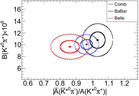
Figure 14: Contours at 1 (solid) and 2 (dotted) $\sigma$ in the $\left|\frac{\overline{A}(\overline{K}^{*0}\pi^{-})}{A(K^{*0}\pi^{+})}\right|$ vs ${\mathcal{B}}(K^{*0}\pi^{+})$ plane for the BABAR (black) and Belle (red) results, as well as the combination (blue).

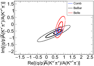
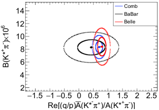
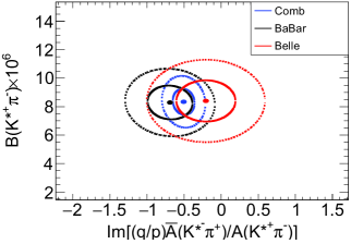
Figure 15: Contours at 1 (solid) and 2 (dotted) $\sigma$ in the ${\mathcal{R}e}\left[\frac{q}{p}\frac{\overline{A}(K^{*-}\pi^{+})}{A(K^{*+}\pi^{-})}\right]$ vs ${\mathcal{I}m}\left[\frac{q}{p}\frac{\overline{A}(K^{*-}\pi^{+})}{A(K^{*+}\pi^{-})}\right]$ (left), ${\mathcal{R}e}\left[\frac{q}{p}\frac{\overline{A}(K^{*-}\pi^{+})}{A(K^{*+}\pi^{-})}\right]$ vs ${\mathcal{B}}(K^{*+}\pi^{-})$ (middle) and ${\mathcal{I}m}\left[\frac{q}{p}\frac{\overline{A}(K^{*-}\pi^{+})}{A(K^{*+}\pi^{-})}\right]$ vs ${\mathcal{B}}(K^{*+}\pi^{-})$ (right) planes for the BABAR (black) and Belle (red) results, as well as the combination (blue).

$B^{+}\rightarrow K^{+}\pi^{-}\pi^{+}$	Value
$\left|\frac{\overline{A}(\overline{K}^{*0}\pi^{-})}{A(K^{*0}\pi^{+})}\right|$	$0.965\pm 0.037$
${\mathcal{B}}(K^{*0}\pi^{+})(\times 10^{-6})$	$10.062\pm 0.835$

$B^{0}\rightarrow K^{0}_{S}\pi^{+}\pi^{-}$	Value	${\mathcal{R}e}\left[\frac{q}{p}\frac{\overline{A}(K^{*-}\pi^{+})}{A(K^{*+}\pi^{-})}\right]$	${\mathcal{I}m}\left[\frac{q}{p}\frac{\overline{A}(K^{*-}\pi^{+})}{A(K^{*+}\pi^{-})}\right]$	${\mathcal{B}}(K^{*+}\pi^{-})$
${\mathcal{R}e}\left[\frac{q}{p}\frac{\overline{A}(K^{*-}\pi^{+})}{A(K^{*+}\pi^{-})}\right]$	$0.698\pm 0.120$	1.00	0.58	-0.01
${\mathcal{I}m}\left[\frac{q}{p}\frac{\overline{A}(K^{*-}\pi^{+})}{A(K^{*+}\pi^{-})}\right]$	$-0.506\pm 0.146$		1.00	-0.09
${\mathcal{B}}(K^{*+}\pi^{-})(\times 10^{-6})$	$8.340\pm 0.910$			1.00

Table 9: Central values of the observables from the $B^{+}\rightarrow K^{+}\pi^{-}\pi^{+}$ (top) and $B^{0}\rightarrow K^{0}_{S}\pi^{+}\pi^{-}$ (bottom) analysis obtained by combining BABAR and Belle results.

These combined results for the $B^{0}\rightarrow K^{0}_{S}\pi^{+}\pi^{-}$ and $B^{+}\rightarrow K^{+}\pi^{-}\pi^{-}$ modes are used with the BABAR results for the $B^{0}\rightarrow K^{+}\pi^{-}\pi^{0}$ and $B^{+}\rightarrow K^{0}_{S}\pi^{+}\pi^{0}$ as inputs for the phenomenological analysis using the current experimental measurements.

Appendix B Two-body non leptonic amplitudes in QCD factorisation

We compute the $B\to K^{*}\pi$ amplitudes in the framework of QCD factorisation, using the results of Ref. Beneke:2003zv . We take the semileptonic $B\to\pi$ and $B\to K\pi$ form factors from computations based on Light-Cone Sum Rules Ball:2004rg ; Straub:2015ica . The parameters for the light-meson distribution amplitudes that enter hard-scattering contributions are consistently taken from the last two references. On the other hand the first inverse moment of the $B$-meson distribution amplitude $\lambda_{B}$ is taken from Ref. Braun:2003wx . Quark masses are taken from review by the FLAG group Aoki:2016frl . Our updated inputs are summarised in Table 10.

Input	Value	Input	Value
$\alpha_{1}(K^{*})$	$0.06\pm 0\pm 0.04$	$\alpha_{1}(K^{*},\perp)$	$0.04\pm 0\pm 0.03$
$\alpha_{2}(K^{*})$	$0.16\pm 0\pm 0.09$	$\alpha_{2}(K^{*},\perp)$	$0.10\pm 0\pm 0.08$
$f_{\perp}(K^{*})$	$0.159\pm 0\pm 0.006$	$A_{0}[B\to K^{*}](0)$	$0.356\pm 0\pm 0.046$
$\alpha_{2}(\pi)$	$0.062\pm 0\pm 0.054$	$F_{0}[B\to\pi](0)$	$0.258\pm 0\pm 0.031$
$\lambda_{B}$	$0.460\pm 0\pm 0.110$	$\bar{m}_{b}$	$4.17$
$\bar{m}_{s}$	$0.0939\pm 0\pm 0.0011$	$m_{q}/m_{s}$	$\sim 0$

Table 10: Input values for the hadronic parameters that enter QCD factorisation predictions: moments of the distribution amplitudes for mesons, decay constants, form factors and quark masses. Dimensionful quantities are in GeV. The $\pm 0$ in second position means that all uncertainties are considered as coming from a theoretical origin and they are treated according to the Rfit approach. See the text for references.

We stress that the calculations of Ref. Beneke:2003zv correspond to Next-to-Leading Order (NLO). Since then, some NNLO contributions have been computed BHWS ; Bell:2007tv ; Bell:2009nk ; Beneke:2009ek ; Bell:2015koa , that we neglect in view of the sizeable uncertainties on the input parameters: this is sufficient for our illustrative purposes (see Section V.3).

Appendix C Reference scenario and prospective studies

Some of the experimental results collected in App. A are affected by large uncertainties, and the central values are not always fully consistent with SM expectations. This is not a problem when we want to extract values of the hadronic parameters from the data, but it makes rather unclear the discussion of the accuracy of specific models (say, for the extraction of weak angles) or the prospective studies assuming improved experimental measurements, see Secs. IV and VI.

For this reason, we design a reference scenario described in Tab. 11. The values on hadronic parameters are chosen to reproduce the current best averages of branching fractions and $CP$ asymmetries in $B\rightarrow K^{*}\pi$ roughly. As most observable phase differences among these modes are poorly constrained by the results currently available, we do no attempt at reproducing their central values and we use the values resulting from the hadronic parameters. The hadronic amplitudes are constrained to respect the naive assumptions: $|P_{\rm EW}/T_{3/2}|\simeq 1.35\%$, $|P^{C}_{\rm EW}|<|P_{\rm EW}|$ and $|T^{00}_{\rm C}|<|T^{+-}|$. The best values of the hadronic parameters yield the values of branching ratios and $CP$ asymmetries gathered in Tab. 11. As can be seen, the overall agreement is fair, but it is not good for all observables. Indeed, as discussed in Sec. V, the current data do not favour all the hadronic hierarchies that we have imposed to obtain our reference scenario in Tab. 11.

For the studies of different methods to extract CKM parameters described in Sec. IV, we fit the values of hadronic parameters by assigning small, arbitrary, uncertainties to the physical observables: $\pm 5\%$ for branching ratios, $\pm 0.5\%$ for $CP$ asymmetries, and $\pm 5^{\circ}$ for interference phases.

For the prospective studies described in Sec. VI, we estimate future experimental uncertainties at two different stages. We first consider a list of expected measurements from LHCb, using the combined Run1 and Run2 data. We then reassess the expected results including Belle II measurements. Our method to project uncertainties in the two stages is based on the statistical scaling of data samples ($1/\sqrt{N_{\rm evts}}$), corrected for additional factors due to particular detector performances and analysis technique features, as described below.

LHCb Run1 and Run2 data will significantly increase the statistics mainly for the fully charged final states $B^{0}\rightarrow K^{0}_{S}(\rightarrow\pi^{+}\pi^{-})\pi^{+}\pi^{-}$ and $B^{+}\rightarrow K^{+}\pi^{-}\pi^{+}$, with an expected increase of about $3$ and $40$, respectively B0toKspipi_LHCb:2012iva ; BtoKpipi_LHCb:2013iva . For these modes, we assume a signal-to-background ratio similar to the ones measured at $B$ factories (this may represent an underestimation of the potential sensitivity of LHCb data, but this assumption has a very minor impact on the results of our prospective study). The statistical scaling factor thus defined can be applied as such to direct $CP$ asymmetries, but some additional aspects must be considered in the scaling of uncertainties for other observables. For time-dependent $CP$ asymmetries, the difference in flavour-tagging performances (the effective tagging efficiency $Q$) should be taken into account. In the $B$-factory environment, a quality factor $Q_{\rm B-factories}\sim 30$ FavourTagging_BaBar:2009iva ; FavourTagging_Belle:2012iva was achieved, while for LHCb a smaller value is used ($Q_{\rm LHCb}\sim 3$ FavourTagging_LHCb:2012iva ), which entails an additional factor $(Q_{\rm B-factories}/Q_{\rm LHCb})^{1/2}\sim 3.2$ in the scaling of uncertainties. For branching ratios, LHCb is not able to directly count the number of $B$ mesons produced, and it is necessary to resort to a normalisation using final states for which the branching ratio has been measured elsewhere (mainly at $B$-factories). This additional source of uncertainty is taken into account in the projection of the error. Finally, in our prospective studies, we adopt the pessimistic view of neglecting potential measurements from LHCb for modes with $\pi^{0}$ mesons in the final state (e.g., $B^{0}\rightarrow K^{+}\pi^{-}\pi^{0}$ and $B^{+}\rightarrow K^{0}_{S}\pi^{+}\pi^{0}$), as it is difficult to anticipate the evolution in the performances for $\pi^{0}$ reconstruction and phase space resolution.

Belle II Urquijo:2015qsa expects to surpass by a factor of $\sim 50$ the total statistics collected by the $B$-factories. As the experimental environments will be very similar, we just scale the current uncertainties by this statistical factor.

Starting from the statistical uncertainties from Babar and scaling them according to the above procedure, we obtain our projections of uncertainties on physical observables, shown in Tab. 12, where the current uncertainties are compared with the projected ones for the first ($B$-factories combined with LHCb Run1 and Run2) and second (adding Belle II) stages described previously.

Hadronic amplitudes	Magnitude	Phase (∘)	Observable	Measurement	Value
$T^{+-}$	2.540	0.0	${\mathcal{B}}(B^{0}\rightarrow K^{*+}\pi^{-})$	$8.4\pm 0.8$	$7.1$
$T^{00}_{\rm C}$	0.762	75.8	${\mathcal{B}}(B^{0}\rightarrow K^{*0}\pi^{0})$	$3.3\pm 0.6$	$1.6$
$N^{0+}$	0.143	108.4	${\mathcal{B}}(B^{+}\rightarrow K^{*+}\pi^{0})$	$8.2\pm 1.8$	$8.5$
$P^{+-}$	0.091	-6.5	${\mathcal{B}}(B^{+}\rightarrow K^{*0}\pi^{+})$	$10.1^{+0.8}_{-0.9}$	$10.9$
$P_{\rm EW}$	0.038	15.2	$A_{CP}(B^{0}\rightarrow K^{*+}\pi^{-})$	$-0.23\pm 0.06$	$-0.129$
$P_{\rm EW}^{\rm C}$	0.029	101.9	$A_{CP}(B^{0}\rightarrow K^{*0}\pi^{0})$	$-0.15\pm 0.13$	$+0.465$
$\left|\frac{V_{ts}V_{tb}^{*}P^{+-}}{V_{us}V_{ub}^{*}T^{+-}}\right|$	1.809		$A_{CP}(B^{+}\rightarrow K^{*+}\pi^{0})$	$-0.39\pm 0.12$	$-0.355$
$\left|T^{00}_{\rm C}/T^{+-}\right|$	0.300		$A_{CP}(B^{+}\rightarrow K^{*0}\pi^{+})$	$+0.038\pm 0.042$	$+0.039$
$\left|N^{0+}/T^{00}_{\rm C}\right|$	0.187
$\left|P_{\rm EW}/P^{+-}\right|$	0.421
$\left|P_{\rm EW}/(T^{+-}+T^{00}_{\rm C})\right|/R$	1.009
$\left|P_{\rm EW}^{\rm C}/P_{\rm EW}\right|$	0.762

Table 11: Values chosen for our reference scenario. The values on hadronic parameters (left columns) are chosen to roughly reproduce the reference values of branching fractions (in units of $10^{-6}$) and $CP$ asymmetries in $B\rightarrow K^{*}\pi$ (right columns). The reference input values come from the current HFLAV averages Amhis:2016xyh , except for $A_{CP}(B^{+}\rightarrow K^{*+}\pi^{0})$, where the value is taken from Ref. Lees:2015uun . The values of the hadronic parameters yield the branching ratios and $CP$ asymmetries of the last column.

Observable	Analysis	Current uncertainty	LHCb (Run1+Run2)	LHCb+Belle II
${\mathcal{R}e}\left[\frac{q}{p}\frac{\overline{A}(K^{*-}\pi^{+})}{A(K^{*+}\pi^{-})}\right]$	$B^{0}\rightarrow K^{0}_{S}\pi^{+}\pi^{-}$	$0.11$	$0.04$	$0.01$
${\mathcal{I}m}\left[\frac{q}{p}\frac{\overline{A}(K^{*-}\pi^{+})}{A(K^{*+}\pi^{-})}\right]$	$B^{0}\rightarrow K^{0}_{S}\pi^{+}\pi^{-}$	$0.16$	$0.11$	$0.02$
${\mathcal{B}}(K^{*+}\pi^{-})$	$B^{0}\rightarrow K^{0}_{S}\pi^{+}\pi^{-}$	$0.69$	$0.32$	$0.09$
$\left|\frac{\overline{A}(K^{*-}\pi^{+})}{A(K^{*+}\pi^{-})}\right|$	$B^{0}\rightarrow K^{+}\pi^{-}\pi^{0}$	$0.06$	$0.06$	$0.01$
${\mathcal{R}e}\left[\frac{A(K^{*0}\pi^{0})}{A(K^{*+}\pi^{-})}\right]$	$B^{0}\rightarrow K^{+}\pi^{-}\pi^{0}$	$0.11$	$0.11$	$0.02$
${\mathcal{I}m}\left[\frac{A(K^{*0}\pi^{0})}{A(K^{*+}\pi^{-})}\right]$	$B^{0}\rightarrow K^{+}\pi^{-}\pi^{0}$	$0.23$	$0.23$	$0.03$
${\mathcal{R}e}\left[\frac{\overline{A}(\overline{K}^{*0}\pi^{0})}{\overline{A}(K^{*-}\pi^{+})}\right]$	$B^{0}\rightarrow K^{+}\pi^{-}\pi^{0}$	$0.10$	$0.10$	$0.01$
${\mathcal{I}m}\left[\frac{\overline{A}(\overline{K}^{*0}\pi^{0})}{\overline{A}(K^{*-}\pi^{+})}\right]$	$B^{0}\rightarrow K^{+}\pi^{-}\pi^{0}$	$0.30$	$0.30$	$0.04$
${\mathcal{B}}(K^{*0}\pi^{0})$	$B^{0}\rightarrow K^{+}\pi^{-}\pi^{0}$	$0.35$	$0.35$	$0.05$
$\left|\frac{\overline{A}(\overline{K}^{*0}\pi^{-})}{A(K^{*0}\pi^{+})}\right|$	$B^{+}\rightarrow K^{+}\pi^{-}\pi^{+}$	$0.04$	$0.005$	$0.004$
${\mathcal{B}}(K^{*0}\pi^{+})$	$B^{+}\rightarrow K^{+}\pi^{-}\pi^{+}$	$0.81$	$0.50$	$0.11$
$\left|\frac{\overline{A}(K^{*-}\pi^{0})}{A(K^{*+}\pi^{0})}\right|$	$B^{+}\rightarrow K^{0}_{S}\pi^{+}\pi^{0}$	$0.15$	$0.15$	$0.02$
${\mathcal{R}e}\left[\frac{A(K^{*+}\pi^{0})}{A(K^{*0}\pi^{+})}\right]$	$B^{+}\rightarrow K^{0}_{S}\pi^{+}\pi^{0}$	$0.16$	$0.16$	$0.02$
${\mathcal{I}m}\left[\frac{A(K^{*+}\pi^{0})}{A(K^{*0}\pi^{+})}\right]$	$B^{+}\rightarrow K^{0}_{S}\pi^{+}\pi^{0}$	$0.30$	$0.30$	$0.04$
${\mathcal{R}e}\left[\frac{\overline{A}(K^{*-}\pi^{0})}{\overline{A}(\overline{K}^{*0}\pi^{-})}\right]$	$B^{+}\rightarrow K^{0}_{S}\pi^{+}\pi^{0}$	$0.21$	$0.21$	$0.03$
${\mathcal{I}m}\left[\frac{\overline{A}(K^{*-}\pi^{0})}{\overline{A}(\overline{K}^{*0}\pi^{-})}\right]$	$B^{+}\rightarrow K^{0}_{S}\pi^{+}\pi^{0}$	$0.13$	$0.13$	$0.02$
${\mathcal{B}}(K^{*+}\pi^{0})$	$B^{+}\rightarrow K^{0}_{S}\pi^{+}\pi^{0}$	$0.92$	$0.92$	$0.13$

Table 12: Prospective scenarios for statistical uncertainties on the $B\rightarrow K^{\star}\pi$ observables. The extrapolations are based on the current statistical uncertainties from BABAR results. The uncertainties on the branching fractions are given in units of $10^{-6}$.

References

- (1) A. J. Bevan et al. [BABAR and Belle Collaborations], Eur. Phys. J. C 74 (2014) 3026 doi:10.1140/epjc/s10052-014-3026-9 [arXiv:1406.6311 [hep-ex]].
- (2) R. Aaij et al. [LHCb Collaboration], Eur. Phys. J. C 73 (2013) no.4, 2373 doi:10.1140/epjc/s10052-013-2373-2 [arXiv:1208.3355 [hep-ex]].
- (3) N. Cabibbo, Phys. Rev. Lett. 10 (1963) 531. doi:10.1103/PhysRevLett.10.531
- (4) M. Kobayashi and T. Maskawa, Prog. Theor. Phys. 49 (1973) 652. doi:10.1143/PTP.49.652
- (5) O. Deschamps et al., work in progress.
- (6) J. Charles et al. [CKMfitter Group], Eur. Phys. J. C 41 (2005) 1 [arXiv:hep-ph/0406184].
- (7) Updates and numerical results on the CKMfitter group web site: http://ckmfitter.in2p3.fr/
- (8) J. Charles et al., Phys. Rev. D 91 (2015) no.7, 073007 doi:10.1103/PhysRevD.91.073007 [arXiv:1501.05013 [hep-ph]].
- (9) P. Koppenburg and S. Descotes-Genon, arXiv:1702.08834 [hep-ex].
- (10) J. Charles, S. Descotes-Genon, Z. Ligeti, S. Monteil, M. Papucci and K. Trabelsi, Phys. Rev. D 89 (2014) no.3, 033016 doi:10.1103/PhysRevD.89.033016 [arXiv:1309.2293 [hep-ph]].
- (11) A. Lenz, U. Nierste, J. Charles, S. Descotes-Genon, H. Lacker, S. Monteil, V. Niess and S. T’Jampens, Phys. Rev. D 86 (2012) 033008 doi:10.1103/PhysRevD.86.033008 [arXiv:1203.0238 [hep-ph]].
- (12) A. Lenz et al., Phys. Rev. D 83 (2011) 036004 doi:10.1103/PhysRevD.83.036004 [arXiv:1008.1593 [hep-ph]].
- (13) O. Deschamps, S. Descotes-Genon, S. Monteil, V. Niess, S. T’Jampens and V. Tisserand, Phys. Rev. D 82 (2010) 073012 doi:10.1103/PhysRevD.82.073012 [arXiv:0907.5135 [hep-ph]].
- (14) M. Beneke, G. Buchalla, M. Neubert and C. T. Sachrajda, Phys. Rev. Lett. 83 (1999) 1914 doi:10.1103/PhysRevLett.83.1914 [hep-ph/9905312].
- (15) M. Beneke, G. Buchalla, M. Neubert and C. T. Sachrajda, Nucl. Phys. B 591 (2000) 313 doi:10.1016/S0550-3213(00)00559-9 [hep-ph/0006124].
- (16) M. Beneke and M. Neubert, Nucl. Phys. B 675 (2003) 333 doi:10.1016/j.nuclphysb.2003.09.026 [hep-ph/0308039].
- (17) M. Beneke, J. Rohrer and D. Yang, Nucl. Phys. B 774 (2007) 64 doi:10.1016/j.nuclphysb.2007.03.020 [hep-ph/0612290].
- (18) H. n. Li, Phys. Rev. D 66 (2002) 094010 doi:10.1103/PhysRevD.66.094010 [hep-ph/0102013].
- (19) H. n. Li and K. Ukai, Phys. Lett. B 555 (2003) 197 doi:10.1016/S0370-2693(03)00049-2 [hep-ph/0211272].
- (20) H. n. Li, Prog. Part. Nucl. Phys. 51 (2003) 85 doi:10.1016/S0146-6410(03)90013-5 [hep-ph/0303116].
- (21) A. Ali, G. Kramer, Y. Li, C. D. Lu, Y. L. Shen, W. Wang and Y. M. Wang, Phys. Rev. D 76 (2007) 074018 doi:10.1103/PhysRevD.76.074018 [hep-ph/0703162 [HEP-PH]].
- (22) H. n. Li, CERN Yellow Report CERN-2014-001, pp.95-135 doi:10.5170/CERN-2014-001.95 [arXiv:1406.7689 [hep-ph]].
- (23) W. F. Wang and H. n. Li, Phys. Lett. B 763 (2016) 29 doi:10.1016/j.physletb.2016.10.026 [arXiv:1609.04614 [hep-ph]].
- (24) C. W. Bauer, D. Pirjol and I. W. Stewart, Phys. Rev. D 67 (2003) 071502 doi:10.1103/PhysRevD.67.071502 [hep-ph/0211069].
- (25) M. Beneke and T. Feldmann, Nucl. Phys. B 685 (2004) 249 doi:10.1016/j.nuclphysb.2004.02.033 [hep-ph/0311335].
- (26) C. W. Bauer, D. Pirjol, I. Z. Rothstein and I. W. Stewart, Phys. Rev. D 70 (2004) 054015 doi:10.1103/PhysRevD.70.054015 [hep-ph/0401188].
- (27) C. W. Bauer, I. Z. Rothstein and I. W. Stewart, Phys. Rev. D 74 (2006) 034010 doi:10.1103/PhysRevD.74.034010 [hep-ph/0510241].
- (28) T. Becher, A. Broggio and A. Ferroglia, Lect. Notes Phys. 896 (2015) doi:10.1007/978-3-319-14848-9 [arXiv:1410.1892 [hep-ph]].
- (29) S. Descotes-Genon and C. T. Sachrajda, Nucl. Phys. B 625 (2002) 239 doi:10.1016/S0550-3213(02)00017-2 [hep-ph/0109260].
- (30) M. Ciuchini, E. Franco, G. Martinelli, M. Pierini and L. Silvestrini, Phys. Lett. B 515 (2001) 33 doi:10.1016/S0370-2693(01)00700-6 [hep-ph/0104126].
- (31) M. Beneke, G. Buchalla, M. Neubert and C. T. Sachrajda, Phys. Rev. D 72 (2005) 098501 doi:10.1103/PhysRevD.72.098501 [hep-ph/0411171].
- (32) A. V. Manohar and I. W. Stewart, Phys. Rev. D 76 (2007) 074002 doi:10.1103/PhysRevD.76.074002 [hep-ph/0605001].
- (33) H. n. Li and S. Mishima, Phys. Rev. D 83 (2011) 034023 doi:10.1103/PhysRevD.83.034023 [arXiv:0901.1272 [hep-ph]].
- (34) F. Feng, J. P. Ma and Q. Wang, arXiv:0901.2965 [hep-ph].
- (35) M. Beneke, G. Buchalla, M. Neubert and C. T. Sachrajda, Eur. Phys. J. C 61 (2009) 439 doi:10.1140/epjc/s10052-009-1028-9 [arXiv:0902.4446 [hep-ph]].
- (36) T. Becher and G. Bell, Phys. Lett. B 713 (2012) 41 doi:10.1016/j.physletb.2012.05.016 [arXiv:1112.3907 [hep-ph]].
- (37) M. Beneke, Nucl. Part. Phys. Proc. 261-262 (2015) 311 doi:10.1016/j.nuclphysbps.2015.03.021 [arXiv:1501.07374 [hep-ph]].
- (38) B. Aubert et al. [BABAR Collaboration], Phys. Rev. D 80 (2009) 112001 doi:10.1103/PhysRevD.80.112001 [arXiv:0905.3615 [hep-ex]].
- (39) B. Aubert et al. [BABAR Collaboration], Phys. Rev. D 78, 012004 (2008) doi:10.1103/PhysRevD.78.012004 [arXiv:0803.4451 [hep-ex]].
- (40) J. P. Lees et al. [BABAR Collaboration], Phys. Rev. D 83, 112010 (2011) doi:10.1103/PhysRevD.83.112010 [arXiv:1105.0125 [hep-ex]].
- (41) J. P. Lees et al. [BABAR Collaboration], arXiv:1501.00705 [hep-ex].
- (42) J. P. Lees et al. [BABAR Collaboration], Phys. Rev. D 84, 092007 (2011) doi:10.1103/PhysRevD.84.092007 arXiv:1109.0143 [hep-ex].
- (43) A. Garmash et al. [Belle Collaboration], Phys. Rev. Letters 96 (2006) 251803 doi:10.1103/PhysRevD.79.072004 [arXiv:0811.3665 [hep-ex]].
- (44) J. Dalseno et al. [Belle Collaboration], Phys. Rev. D 79 (2009) 072004 doi:10.1103/PhysRevD.79.072004 [arXiv:0811.3665 [hep-ex]].
- (45) B. Bhattacharya, M. Gronau and J. L. Rosner, Phys. Lett. B 726 (2013) 337 doi:10.1016/j.physletb.2013.08.062 [arXiv:1306.2625 [hep-ph]].
- (46) B. Bhattacharya and D. London, JHEP 1504 (2015) 154 doi:10.1007/JHEP04(2015)154 [arXiv:1503.00737 [hep-ph]].
- (47) B. Bhattacharya, M. Gronau, M. Imbeault, D. London and J. L. Rosner, Phys. Rev. D 89 (2014) no.7, 074043 doi:10.1103/PhysRevD.89.074043 [arXiv:1402.2909 [hep-ph]], and references therein
- (48) J. H. Alvarenga Nogueira et al., arXiv:1605.03889 [hep-ex].
- (49) K. Abe et al. [Belle Collaboration], arXiv:0708.1845 [hep-ex].
- (50) B. Aubert et al. [BaBar Collaboration], Phys. Rev. D 76 (2007) 071101 doi:10.1103/PhysRevD.76.071101 [hep-ex/0702010].
- (51) L. A. Pérez Pérez, “Time-Dependent Amplitude Analysis of decays with the BABAR Experiment and constraints on the CKM matrix using the and modes,” TEL-00379188.
- (52) Y. Nir and H. R. Quinn, Phys. Rev. Lett. 67 (1991) 541. doi:10.1103/PhysRevLett.67.541
- (53) M. Gronau and J. Zupan, Phys. Rev. D 71 (2005) 074017 doi:10.1103/PhysRevD.71.074017 [hep-ph/0502139].
- (54) F. J. Botella and J. P. Silva, Phys. Rev. D 71 (2005) 094008 doi:10.1103/PhysRevD.71.094008 [hep-ph/0503136].
- (55) M. Beneke and S. Jäger, Nucl. Phys. B 768 (2007) 51 doi:10.1016/j.nuclphysb.2007.01.016 [hep-ph/0610322].
- (56) G. Bell and V. Pilipp, Phys. Rev. D 80 (2009) 054024 doi:10.1103/PhysRevD.80.054024 [arXiv:0907.1016 [hep-ph]].
- (57) G. Bell, M. Beneke, T. Huber and X. Q. Li, Phys. Lett. B 750 (2015) 348 doi:10.1016/j.physletb.2015.09.037 [arXiv:1507.03700 [hep-ph]].
- (58) F. J. Botella, D. London and J. P. Silva, Phys. Rev. D 73 (2006) 071501 doi:10.1103/PhysRevD.73.071501 [hep-ph/0602060].
- (59) M. Gronau and D. London, Phys. Rev. Lett. 65 (1990) 3381. doi:10.1103/PhysRevLett.65.3381
- (60) A. J. Buras and R. Fleischer, Eur. Phys. J. C 11 (1999) 93 doi:10.1007/s100529900201, 10.1007/s100520050617 [hep-ph/9810260].
- (61) M. Neubert and J. L. Rosner, Phys. Lett. B 441 (1998) 403 doi:10.1016/S0370-2693(98)01194-0 [hep-ph/9808493].
- (62) M. Neubert and J. L. Rosner, Phys. Rev. Lett. 81 (1998) 5076 doi:10.1103/PhysRevLett.81.5076 [hep-ph/9809311].
- (63) M. Gronau, Phys. Rev. Lett. 91 (2003) 139101 doi:10.1103/PhysRevLett.91.139101 [hep-ph/0305144].
- (64) M. Ciuchini, M. Pierini and L. Silvestrini, Phys. Rev. D 74 (2006) 051301 doi:10.1103/PhysRevD.74.051301 [hep-ph/0601233].
- (65) M. Gronau, D. Pirjol, A. Soni and J. Zupan, Phys. Rev. D 75 (2007) 014002 doi:10.1103/PhysRevD.75.014002 [hep-ph/0608243].
- (66) Y. Amhis et al., arXiv:1612.07233 [hep-ex].
- (67) J. Charles, S. Descotes-Genon, V. Niess and L. Vale Silva, arXiv:1611.04768 [hep-ph].
- (68) R. Aaij et al. [LHCb Collaboration], Phys. Rev. D 90, no. 11, 112004 (2014) doi:10.1103/PhysRevD.90.112004 [arXiv:1408.5373 [hep-ex]].
- (69) P. Urquijo, Nucl. Part. Phys. Proc. 263-264, 15 (2015). doi:10.1016/j.nuclphysbps.2015.04.004. Belle II web page: https://www.belle2.org/
- (70) R. Aaij et al. [LHCb Collaboration], Phys. Rev. Lett. 111 (2013) 101801 [arXiv:1306.1246 [hep-ex]].
- (71) LHCb-CONF-2012-023, July 6, 2012
- (72) LHCb-CONF-2012-026, July 11, 2012
- (73) B. Aubert et al. [BABAR Collaboration], Phys. Rev. D 79, (2009) 072009 doi:10.1103/PhysRevD.79.072009 [arXiv:0902.1708 [hep-ex]].
- (74) I. Adachi et al. [Belle Collaboration], Phys. Rev. Lett. 108, 171802 (2012) doi:10.1103/PhysRevLett.108.171802 [arXiv:1201.4643 [hep-ex]].
- (75) P. Ball and R. Zwicky, Phys. Rev. D 71 (2005) 014029 doi:10.1103/PhysRevD.71.014029 [hep-ph/0412079].
- (76) A. Bharucha, D. M. Straub and R. Zwicky, JHEP 1608 (2016) 098 doi:10.1007/JHEP08(2016)098 [arXiv:1503.05534 [hep-ph]].
- (77) V. M. Braun, D. Y. Ivanov and G. P. Korchemsky, Phys. Rev. D 69 (2004) 034014 doi:10.1103/PhysRevD.69.034014 [hep-ph/0309330].
- (78) S. Aoki et al., Eur. Phys. J. C 77 (2017) no.2, 112 doi:10.1140/epjc/s10052-016-4509-7 [arXiv:1607.00299 [hep-lat]].
- (79) G. Bell, talk given at the workshop Future Challenges in Non-Leptonic B Decays: Theory and Experiment, Bad Honnef (Germany), 10-12 February 2016 [https://indico.cern.ch/event/458285/].
- (80) G. Bell, Nucl. Phys. B 795 (2008) 1 doi:10.1016/j.nuclphysb.2007.09.006 [arXiv:0705.3127 [hep-ph]].
- (81) G. Bell, Nucl. Phys. B 822 (2009) 172 doi:10.1016/j.nuclphysb.2009.07.012 [arXiv:0902.1915 [hep-ph]].
- (82) M. Beneke, T. Huber and X. Q. Li, Nucl. Phys. B 832 (2010) 109 doi:10.1016/j.nuclphysb.2010.02.002 [arXiv:0911.3655 [hep-ph]].