Optimized Gillespie algorithms for the simulation of Markovian epidemic processes on large and heterogeneous networks

Abstract

Numerical simulation of continuous-time Markovian processes is an essential and widely applied tool in the investigation of epidemic spreading on complex networks. Due to the high heterogeneity of the connectivity structure through which epidemics is transmitted, efficient and accurate implementations of generic epidemic processes are not trivial and deviations from statistically exact prescriptions can lead to uncontrolled biases. Based on the Gillespie algorithm (GA), in which only steps that change the state are considered, we develop numerical recipes and describe their computer implementations for statistically exact and computationally efficient simulations of generic Markovian epidemic processes aiming at highly heterogeneous and large networks. The central point of the recipes investigated here is to include phantom processes, that do not change the states but do count for time increments. We compare the efficiencies for the susceptible-infected-susceptible, contact process and susceptible-infected-recovered models, that are particular cases of a generic model considered here. We numerically confirm that the simulation outcomes of the optimized algorithms are statistically indistinguishable from the original GA and can be several orders of magnitude more efficient.

1 Introduction

Our daily life is ubiquitously ruled by networked systems [1, 2, 3, 4] as the transportation infrastructure through which we move, social media in which we get informed, the biochemical networks regulating the cell processes inside our bodies, the connections of neurons of our brain, which are just a few examples. In the last two decades, we have advanced significantly in the understanding of the structure and functioning of networks [1, 2], but we still have immense challenges in the theoretical frameworks for the dynamic processes, such as epidemic spreading, evolving on the top of these networked complex systems [2, 5], which are mostly large and highly heterogeneous [2]. Approximated theories for the epidemic spreading in complex networks have been intensively investigated in the last two decades [6] and computer simulations became fundamental tools to corroborate or to point out the limitations of the theories as well as to provide physical insights in the construction of new ones. So, accurate and efficient simulation methods have become imperative for the progress of this field. Particularly, many real and synthetic networks are very large and heterogeneous [1, 2, 4] requiring algorithms which are simultaneously accurate and efficient.

Epidemic models on networks [6] assume that individuals of a population are represented by vertices while the infection can be transmitted through edges connecting them. Simulations of very large systems have played a key role in the understanding of central issues of epidemic spreading on highly heterogeneous networks. Most of these studies involve thresholds separating an absorbing, disease-free state and an active phase where epidemics can thrive and, thus, this problem can be suited in the framework of absorbing-state phase transitions [6, 7, 8]. The location and the existence of a finite epidemic threshold [9, 10, 11, 12, 13, 14, 15] and the exponents describing the dynamics near the transition [16, 17, 18, 19, 20] have recently been matter of intense discussions fomented by numerical simulations on networks with power-law degree distributions.

Continuous-time Markovian processes can be simulated using the statistically exact Gillespie algorithm (GA) [21, 22], and epidemic processes are not different [23, 24]. To apply GA to epidemics, one must decompose the dynamics into independent spontaneous processes and then perform a change of state by time step that, in turn, is not fixed. However, every time the state of a vertex changes, the list of all spontaneous processes must be updated, a task that can be computationally prohibitive for large networks. Epidemic models are also frequently implemented using synchronous schema [25, 26, 27, 28], in which all vertices are updated simultaneously. The time is discretized in intervals $\delta t$ and the transition rates $\nu$ are converted into probabilities $p=\nu\delta t$. This prescription is exact only for infinitesimal $\delta t$, which is computationally inaccessible, and large discrepancies with statistically exact versions are observed if $\delta t$ is not sufficiently small [23, 29].

In this paper, we discuss statistically exact algorithms derived from GA for efficient simulations of generic Markovian epidemic processes on large complex networks. This algorithm has been applied to investigate the susceptible-infected-susceptible (SIS) (see Sec. 6.1) epidemic model  [10, 11, 12, 13, 15, 30, 31, 32, 33] but, as far we know, an explicit comparison with GA and, therefore, their statistical exactness has not been assessed. The central difference between GA and the other algorithms presented here is that the latter permit steps where no change of configuration takes place, called of phantom processes, which can hugely reduce the computational time. The algorithms studied here were conceived to be implemented in diverse programming languages. Codes in Fortran and Python, which can be translated to other languages, for the fundamental susceptible-infected-susceptible (SIS) model were made available in open access repositories [34].

We briefly review some basic concepts of network theory and the analysis of epidemics on finite networks as an absorbing-state phase transition in sections 2 and 3, respectively. Despite of its seminality, the GA is not sufficiently known in statistical physics and network science communities as we think it should be. Thus, in section 4 we also briefly review the GA and present the central proofs needed to its derivation that will help to understand the optimized algorithms to simulate generic epidemic processes developed in section 5. We further improve these algorithms to specific epidemic models in sections 6.1, 6.2, and 6.3 for SIS, contact process [16], and SIR (susceptible-infected-recovered) [6], respectively, the first two presenting steady active states while the last one does not. Algorithms for more sophisticated epidemic processes [15] are presented in subsection 6.4. We finally draw our concluding remarks in section 7.

2 Networks as substrates for epidemics spreading

In this section, we review some basic concepts of network theory that are used in the implementation of the algorithms for the simulations of epidemics. Comprehensive texts can be found elsewhere [1, 2, 5, 7]. Unweighted and undirected networks are composed by a set of $N$ vertices, labeled by $i=1,2,\cdots,N$, and a set of $E$ unordered pairs $(i,j)$ forming the edges. Weights and directions can be included through infection rates; see section 5. The adjacency matrix is defined as $A_{ij}=1$ if there exists an edge connecting $i$ and $j$ (they are neighbors) and $A_{ij}=0$ otherwise.

The degree of a vertex $i$ is the number of edges connecting it to other vertices and is given by $k_{i}=\sum_{j}A_{ij}$. The degree of the most and the less connected vertices of the network are represented by $k_{\text{max}}$ and $k_{\text{min}}$, respectively. The degree distribution $P_{s}(k)$ of a single network realization is the probability that a randomly selected vertex of the network has degree $k$ and its moments

$$\langle{k^{n}}\rangle=\sum_{k=k_{\text{min}}}^{k_{\text{max}}}k^{n}P_{s}(k)=\frac{1}{N}\sum_{i=1}^{N}k_{i}^{n}$$ (1)

are basic quantities that provide valuable statistical properties of the network. A hub is a vertex with a very large degree compared with the average: $k\gg\langle{k}\rangle$. Outliers are vertices, usually hubs, with degree given by $NP(k)\ll 1$ in an ensemble of networks with the expected degree distribution $P(k)$, implying that only a few of them are observed in a network realization.

Adjacency matrix of networks with a finite average degree $\langle{k}\rangle$ are highly sparse and can be efficiently stored and accessed using the adjacency list [1], which is a one-dimensional array with $\sum_{i=1}^{N}k_{i}$ elements. The neighbors of the vertex $i$ are stored between indexes ${p_{i}}$ and ${p_{i}+k_{i}-1}$, where $p_{1}=1$ and $p_{i}=1+\sum_{j=1}^{i-1}k_{i}$ for $i>1$.

There exist several fundamental models of networks [1, 2]. Here, we will consider the configuration model with a predefined sequence of degrees in which edges are formed to preserve the degree sequence [35]. We can then elect a form of the ensemble degree distribution $P(k)$, $k=k_{0},\cdots,k_{c}$ where $k_{0}$ and $k_{c}$ are lower and upper cutoffs, respectively, and the degree of each vertex is a random number generated according to this distribution [36], forming a sequence $(k_{1},\cdots,k_{i},\cdots,k_{N})$ of disconnected stubs in each vertex $i$. Edges are formed by randomly choosing two stubs and connecting them.

Consider power-law (PL) distributions $P(k)\sim k^{-\gamma}$ bounded by $k\in[k_{0},N]$ where the network size $N$ is large. Using extreme value theory, one can show that the mean value of largest degree $k_{\text{max}}$ scales with network size as [37]

$$\langle{k_{\text{max}}}\rangle\sim N^{\frac{1}{\gamma-1}},$$ (2)

introducing an average natural cutoff in the degree distribution. The fluctuations of $k_{\text{max}}$ are very large [38] and $\langle{k_{\text{max}}}\rangle$ is not necessarily representative of the maximal degree of a network realization.

If multiple and self-connections are rejected, the random selection of stubs to connect generates degree correlations in PL networks with degree exponent $\gamma<3$ [37]. A sufficient condition to eliminate degree correlations in random networks is to impose a cutoff [37] $k\leq(\langle{k}\rangle N)^{1/2}$. This result led to the uncorrelated configuration model (UCM) [39], in which the structural upper cutoff $k_{c}=\sqrt{N}$ was adopted. For $\gamma<3$, an extreme value theory shows that the fluctuations of $k_{\text{max}}$ in UCM networks are relatively small and its value becomes sharply peaked around $k_{c}$. For $\gamma>3$, we have that the fluctuations of $k_{\text{max}}$ diverge as $N^{1/(\gamma-1)}$ [13, 37, 38] implying in large fluctuations of $k_{\text{max}}$ and the presence of outliers.

Outliers play important roles on the efficiencies of the simulations. For SIS, for example, a single outlier can induce a metastable localized phase [13, 31] that makes the simulations computationally much slower. We will discuss the role of outliers in SIS simulations in subsection 6.1. Therefore, for comparisons of efficiencies as functions of the network size we will consider a rigid cutoff defined as [7] $NP(k_{c})=1$ such that $k_{\text{max}}\sim N^{1/\gamma}$ and presents negligible fluctuations in $k_{\text{max}}$ also for $\gamma>3$. This cutoff is suitable to evaluate computational efficiencies because the simulation times for different network samples become essentially the same. Note that this rigid cutoff also renders uncorrelated networks since $N^{1/\gamma}\ll N^{1/2}$ for $\gamma>2$ and the networks with this cutoff will also be referred as UCM hereafter.

So far we have assumed that the graphs do not evolve, considering only quenched networks. On the opposite extreme lay the annealed networks where the connections are rewired at a rate much larger than the rates of the processes taking place on them [7]. The adjacency matrix for an annealed network is defined as the probability that a vertex $i$ is connected to the vertex $j$ in a given time [7]. We associate $k_{i}$ stubs to the vertex $i$. In an uncorrelated model, a stub can be momentarily connected with any stub of the network with equal chance including those belonging to the same vertex [38]. In this model the adjacency matrix becomes

$$A^{\text{ann}}_{ij}=\frac{k_{i}k_{j}}{\sum_{l=1}^{N}k_{l}}=\frac{k_{i}k_{j}}{N\langle{k}\rangle}.$$ (3)

The computer implementation of uncorrelated annealed networks is simple. We need a list with $\sum_{i=1}^{N}k_{i}$ elements containing $k_{i}$ copies of each vertex $i$. The selection of a neighbor of any vertex consists in choosing at random one element of this list. We will use annealed networks to introduce epidemics in the realm of absorbing-state phase transitions in section 3. Algorithms for epidemic processes on annealed networks are adapted versions of those for quenched networks and will not be discussed further.

3 Epidemics in finite networks as an absorbing-state phase transition

In closed systems, states where the disease is eradicated are called absorbing since once one of them is visited, the dynamics remains frozen in such a state forever. Therefore, a state without infected individuals is an absorbing one, since infection can only be produced through interactions involving infected and susceptible pairs.

A paradigmatic epidemic model exhibiting an absorbing-state phase transition is the SIS [40]. The model rules are the following. Vertices can be infected (denoted by I and $\sigma_{i}=1$) or susceptible (S and $\sigma_{i}=0$). The infected individuals spontaneously heal with rate $\mu$. A vertex $i$ can transmit the disease to a susceptible neighbor $j$ with rate $\lambda_{ij}=\lambda A_{ij}$, which means that an infected vertex infects each one of its susceptible neighbors with rate $\lambda$ irrespective of how many it has. This infection rule has deep impacts on the behavior of the SIS model. A noticeable one is the absence of a finite epidemic threshold for a PL degree distribution as the network size goes to infinity [9, 12]. However, thresholds of the SIS model can still be numerically determined for finite sizes [10, 15]; see Fig. 1.

In order to illustrate the epidemic spreading as an absorbing-state phase transition, let us start with the SIS on an arbitrary graph of size $N$ and adjacency matrix elements $A_{ij}$. The total infection rate of the network is given by

$$L=\lambda\sum_{i,j=1}^{N}A_{ij}\sigma_{i}(1-\sigma_{j}),$$ (4)

while the total healing rate is

$$M=\mu\sum_{i=1}^{N}\sigma_{i}=\mu N_{\text{I}},$$ (5)

where $N_{\text{I}}$ is the number of infected vertices. Now, let us consider the simple case of an annealed network with a homogeneous degree distribution $P(s)=\delta_{s,k}$, that leads to the annealed adjacency matrix $A^{\text{ann}}_{ij}=k/N$, which is introduced in Eq. (4) to obtain a total infection rate

$$L=\lambda kN_{\text{I}}\left(1-\frac{N_{\text{I}}}{N}\right).$$ (6)

Therefore, both total rate of infection and healing of this model are functions of the number of infected vertices and does not depend on the specific state.

Let $P_{n}(t)$ be the probability that there are $n$ infected individuals at time $t$ and $W_{nm}$ the transition rate from a state with $m$ to another with $n$ infected vertices. The time evolution of $P_{n}(t)$ is given by the master equation [41]

$$\frac{dP_{n}}{dt}=\sum_{m=0}^{N}[W_{nm}P_{m}-W_{mn}P_{n}],$$ (7)

with rates

$$W_{n+1,n}=g(n)=\lambda kn\left(1-\frac{n}{N}\right)$$ (8)

and

$$W_{n-1,n}=r(n)=\mu n.$$ (9)

The transition rates are zero otherwise.

Plugging Eqs. (8) and (9) in (7) leads to

$$\frac{d\langle{n}\rangle}{dt}=\langle{g(n)}\rangle-\langle{r(n)}\rangle,$$ (10)

where $\langle{f(n)}\rangle=\sum_{n}f(n)P_{n}$. Neglecting fluctuations by assuming that $\langle{g(n)}\rangle\approx g(\langle{n}\rangle)$, the density of infected vertices defined by $\rho=\langle{n}\rangle/N$ evolves as

$$\frac{d\rho}{dt}=(\lambda k-\mu)\rho-\lambda k\rho^{2},$$ (11)

which is easily solved providing the stationary solution

$${\rho}^{*}=\left\{\begin{matrix}\frac{\lambda k-\mu}{\lambda k}\sim(\lambda-\lambda_{c})^{\beta}&,&\lambda\geq\mu/k\\ 0&,&\lambda<\mu/k\end{matrix}\right.,$$ (12)

defining an epidemic threshold $\lambda_{c}=\mu/k$ and an exponent $\beta=1$.

Despite of the approximated solution neglecting fluctuations predicted an absorbing-state phase transition, one can easily verify that a stationary (normalized) solution of the master equation (7) with rates given by Eqs. (8) and (9) is $P_{n}=\delta_{n,0}$, irrespective of $\lambda$ and $\mu$. For a finite system the stationary solution is unique if $W_{nm}$ forms a irreducible matrix [41], which is the present case. So, for finite sizes, this epidemics always visits the absorbing state at a sufficiently long time since the unique true stationary state is the absorbing one. This is a universal feature of closed systems with absorbing states [8].

Stochastic simulations of epidemic processes can only be performed with finite systems and since we do not know the epidemic threshold a priori, we are not able to determine with certainty if the absorbing state was reached because the infection rate is below the epidemic threshold or due to the finite size. To handle these difficulties involving finite sizes and absorbing states, the standard procedure is to use the standard quasistationary (QS) analysis [8] where the averages at time $t$ are constrained to the samples that did not visit an absorbing configuration up to time $t$, and then to consider a finite-size analysis to extrapolate the thermodynamic limit. Here, however, we will adopt a simpler method that just prevents the system from falling into the absorbing state using a reflecting boundary at $n=0$, in which the dynamics returns to the state that it was immediately before visiting the absorbing state. The comparison with the standard QS method in complex networks was recently performed [42]. It has been shown that this method may provide finite size scaling exponents different from the standard QS depending on the network and epidemic model, but preserves the central properties: Below the epidemic threshold the density of infected vertices vanishes as $\rho\sim 1/N$ and above it $\rho$ converges to the actual active stationary value of the infinite system. For the proposal of this work of comparing the accuracy and efficiency of distinct algorithms this simpler method is suitable.

The $s$th order moment of the QS density of infected vertices is defined as

$$\left[{\rho^{s}}\right]=\frac{1}{N^{s}}\sum_{n=1}^{N}n^{s}\bar{P}_{n},$$ (13)

where $\bar{P}_{n}$ is the QS probability that system has $n$ infected vertices computed after a relaxation time $t_{\text{r}}$ during an averaging time $t_{\text{av}}$. In our notation, $\left[{\cdots}\right]$ represents the QS averages and we use $\langle{\cdots}\rangle$ only for the standard ones.

We will use the dynamical susceptibility [10] defined as

$$\left[{\chi}\right]=N\frac{\left[{\rho^{2}}\right]-\left[{\rho}\right]^{2}}{\left[{\rho}\right]},$$ (14)

which provides a pronounced peak at the epidemic threshold for networks without outliers [13], as shown in Fig. 1.

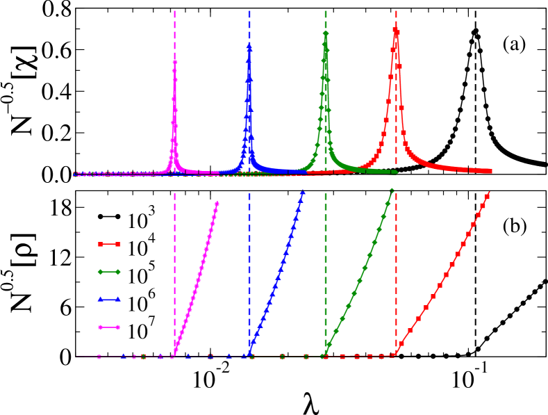
Figure 1: Quasistationary (a) susceptibility and (b) density divided and multiplied, respectively, by $\sqrt{N}$ (to improve visibility) against infection rate $\lambda$ for $\mu=1$ and different network sizes indicated in the legends. The network has a PL degree distribution with $\gamma=2.3$ and rigid cutoff $k_{c}\sim N^{1/\gamma}$. Note that the susceptibility peak coincides with the point where density becomes appreciable indicated by dashed lines.

4 The Gillespie Algorithm

In general, epidemic Markovian processes on graphs can be composed by a set of $Z$ independent spontaneous processes $p=1,2,\cdots,Z$ with rates $\nu_{1},\nu_{2},\cdots,\nu_{Z}$ and the probability that the $p$th process occurs in the infinitesimal interval $[t,t+dt]$ is $\nu_{p}dt$. For example, for the SIS model in a state with $N_{\text{I}}$ infected vertices and $N_{\text{IS}}$ edges pointing from an infected to a susceptible vertex, we can define $Z=N_{\text{I}}+N_{\text{IS}}$ independent processes with rates $\nu_{p}=\mu$ for $p=1,\ldots,N_{\text{I}}$, corresponding to transitions I$\rightarrow$S, and $\nu_{p}=\lambda$ for $p=N_{\text{I}}+1,\ldots,Z$ for the transitions IS$\rightarrow$II.

Spontaneous process is given by the master equation $\frac{dP_{0}}{dt}=-\nu P_{0}$ and $\frac{dP_{1}}{dt}=\nu P_{0}$ with initial condition $P_{j}(0)=\delta_{j0}$, in which $P_{0}(t)$ is the probability that the process has not happen until time $t$ and $P_{1}(t)$ is the probability that it has. The solution is $P_{0}(t)=e^{-\nu t}$ and $P_{1}(t)=1-e^{-\nu t}$.

Consider now $Z$ independent spontaneous processes at time $t$. The probability that the next process is $p$ and that it will happen within the interval $[t+\tau,t+\tau+dt]$ is given by

$$\left(\prod\limits_{q=1}^{Z}e^{-\nu_{q}\tau}\right)\nu_{p}dt=\frac{\nu_{p}}{R}Re^{-R\tau}dt,$$ (15)

where the product is the probability that no transition has happened in the interval $[t,t+\tau]$ and $R=\sum_{q=1}^{Z}\nu_{q}$ is the total rate of transitions. The right-hand side of Eq. (15) is suitably arranged to permit the following interpretation. The next event will take place after a time $\tau$ with an exponential distribution

$$P_{R}(\tau)=Re^{-R\tau}$$ (16)

and this event will be $p$ with probability $\nu_{p}/R$. Given the memoryless Markovian nature of the processes, once a transition has occurred the list of spontaneous processes must be updated but the sequence of the dynamics obeys the same rules.

Based on these ideas the GA algorithm is proposed as follows: 1) Build a list with all spontaneous processes and their respective rates; 2) Select the time step size $\tau$ from the exponential distribution $P_{R}(\tau)$ as $\tau=-\ln(u)/R$, where $u$ is a pseudo random number uniformly distributed in the interval $(0,1)$; 3) Choose the spontaneous process $p$ to take place with probability $\nu_{p}/R$, implement it and update the state of the system; 4) Increment time as $t\rightarrow t+\tau$; 5) Return to step 1. Details of the computer implementation of the GA for epidemics is given in subsection 5.1. It is worth to stress that GA is a statistically exact method.

Let us exemplify GA with the important problem of the SIS dynamics on a star graph, which is composed by $j=1,\ldots,k$ vertices of degree 1, called leaves, connected to a vertex of degree $k$, the center. The state is determined by the number of infected leaves and the state of the center. Let $P(n,\sigma)$ be the probability that there are $n=0,1,\ldots,k$ infected leaves and the center is in either the states $\sigma=0$ (susceptible) or $1$ (infected). The transitions and the respective rates are

$$\begin{matrix}(n,0)&\xrightarrow{\lambda n}&(n,1)\\ (n,0)&\xrightarrow{\mu n}&(n-1,0)\\ (n,1)&\xrightarrow{\lambda(k-n)}&(n+1,1)\\ (n,1)&\xrightarrow{\mu}&(n,0)\\ (n,1)&\xrightarrow{\mu n}&(n-1,1)\end{matrix}$$ (17)

The master equation for this process is a set of $2k$ equations that we numerically integrated using forth order Runge-Kutta method [36]. This stochastic dynamics can be decomposed into four independent spontaneous events: a leaf is healed with rate $\nu_{1}=\mu n$; the center is healed with rate $\nu_{2}=\mu\sigma$; the center is infected with rate $\nu_{3}=\lambda n(1-\sigma)$; and a leaf is infected with rate $\nu_{4}=\lambda(k-n)\sigma$. In Fig. 2, we compare the probability distribution $P(n,\sigma)$ obtained using GA simulations with the numerical integration of the master equation, showing that the results are completely equivalent, as expected.

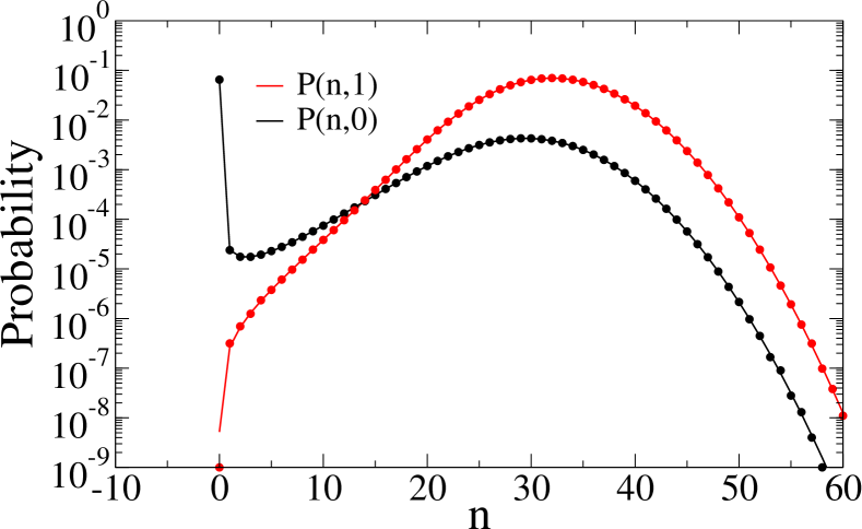
Figure 2: Probability distribution for SIS dynamics on a star graph with $k=100$ leaves at $t=10$ for an infection rate $\lambda=0.5$ and $\mu=1$. The initial condition is the center infected and all leaves susceptible. Symbols are GA simulations ($10^{7}$ samples) and lines are numerical integrations of the master equation.

5 Building algorithms for generic epidemic models

A generic epidemic dynamics can be modeled by assuming that the individuals are in different epidemiological states [43]: susceptible (denoted by S and $\sigma_{i}=0$) that can acquire the infection; infected (I and $\sigma_{i}=1$) and able to transmit the disease to a susceptible contact; or recovered (R and $\sigma_{i}=2$) representing an immunized state where the individual cannot neither transmit or acquire the disease. The generalization to a higher number of epidemiological compartments is straightforward. We consider an unweighted network with adjacency matrix $A_{ij}$. An infected vertex $i$ becomes spontaneously recovered at rate $\mu_{i}$, transmits the infection to vertex $j$ with rate $\lambda_{ij}$ and, if recovered, turns again to a susceptible state (waning immunity [43]) with rate $\alpha_{i}$.

The algorithms require dynamical lists which are represented by capital calligraphic letters. In both the standard (subsection 5.1) and optimized (subsection 5.2) GAs for the generic epidemic process, we build and constantly update two lists $\mathcal{V}^{\text{(I)}}$ and $\mathcal{M}$ with the positions (labels of the vertices) $\mathcal{V}^{\text{(I)}}_{p}$ and recovering rates $\mathcal{M}_{p}$ of the $p=1,\ldots,N_{\text{I}}$ infected vertices. The list updates are simple: the entries of a new infected vertex are added in their ends. When an infected vertex is chosen using $\mathcal{V}^{\text{(I)}}$ and becomes recovered (or susceptible if $\alpha_{i}=\infty$), the last entries of the lists are moved to the index $p$ of the selected vertex, and the list sizes are shortened by 1. Similarly, we build and keep updated the lists $\mathcal{V}^{\text{(R)}}$ and $\mathcal{A}$, with the positions $\mathcal{V}^{\text{(R)}}_{p}$ and rates $\mathcal{A}_{p}$ of the $p=1,\ldots,N_{\text{R}}$ recovered vertices. We also keep updated the total rate that infected vertices are recovered and that recovered ones become susceptible, which are given by

$$M=\sum_{i=1}^{N}\mu_{i}\delta(\sigma_{i},1)=\sum_{p=1}^{N_{\text{I}}}\mathcal{M}_{p}$$ (18)

and

$$A=\sum_{i=1}^{N}\alpha_{i}\delta(\sigma_{i},2)=\sum_{p=1}^{N_{\text{R}}}\mathcal{A}_{p},$$ (19)

respectively, where $\delta(a,b)$ is the delta Kronecker symbol. The update of $M$ or $A$ is done by adding (subtracting) $\mathcal{M}_{p}$ or $\mathcal{A}_{p}$ when a new element is added (removed) in $\mathcal{V}^{\text{(I)}}$ or $\mathcal{V}^{\text{(R)}}$, respectively.

5.1 Implementation of the Gillespie Algorithm

To implement the GA, we need the lists $\mathcal{V}^{\text{(IS)}}$ and $\mathcal{L}$, with the positions $\mathcal{V}^{\text{(IS)}}_{p}$ of the susceptible vertices and infection rates $\mathcal{L}_{p}$ involving the $p=1,\ldots,N_{\text{IS}}$ edges connecting infected and susceptible vertices. It worths to remark that a same susceptible vertex $i$ will appear $n_{i}$ times in the list $\mathcal{V}^{\text{(IS)}}$, where $n_{i}$ is its number of infected neighbors. Due to the multiplicity of edges to be added and deleted from the list every time a change of state occurs, both $\mathcal{V}^{\text{(IS)}}$ and $\mathcal{L}$ are rebuilt and the total infection

$$L=\sum_{i,j=1}^{N}\lambda_{ij}\delta(\sigma_{i},1)\delta(\sigma_{j},0)=\sum_{p=1}^{N_{\text{IS}}}\mathcal{L}_{p}$$ (20)

is computed after each event visiting only the infected vertices and their neighbors with the aid of $\mathcal{V}^{\text{(I)}}$.

With these three lists, the steps of GA (cf. section 4) can be implemented as follows. The total rate of spontaneous processes is $R=M+A+L$. With probabilities $m=M/R$, $a=A/R$, and $l=L/R$ we choose the class of event I$\rightarrow$R, R$\rightarrow$S, or IS$\rightarrow$II, respectively. If the event is a recovering I$\rightarrow$R, one element $p$ of $\mathcal{V}^{\text{(I)}}$ is chosen with probability proportional to $\mathcal{M}_{p}$ and the respective infected vertex is recovered. If a waning of immunity R$\rightarrow$S was selected, one element $p$ of $\mathcal{V}^{\text{(R)}}$ is chosen with probability proportional to $\mathcal{A}_{p}$ and the recovered vertex becomes susceptible. Finally, if an infection event IS$\rightarrow$II was selected, one element $p$ of $\mathcal{V}^{\text{(IS)}}$ is selected with probability proportional to $\mathcal{L}_{p}$ and the susceptible vertex is infected. The time is incremented by $\tau$ drawn from the distribution $P_{R}(\tau)$ given by Eq. (16).

The choice of the events proportionally to $\mathcal{M}_{p}$, $\mathcal{A}_{p}$, and $\mathcal{L}_{p}$ can be implemented using the rejection method, in which an event $p$ is selected with equal chance and accepted with probability $\nu_{p}/\nu_{\text{max}}$ where $\nu_{\text{max}}$ is the largest rate in the corresponding kind of event. The rejection is iteratively repeated until a choice is accepted. It is simpler and usually more efficient to adopt $\mu_{\text{max}}=\max\limits_{i}\{\mu_{i}\}$, $\alpha_{\text{max}}=\max\limits_{i}\{\alpha_{i}\}$, and $\lambda_{\text{max}}=\max\limits_{ij}\{\lambda_{ij}\}$ along the whole network instead of to update this value after every step.

The implementation of the infection events in this GA follows an edge-based while the healing and waning of immunity use a vertex-based update scheme. Alternatively, all events could be performed with vertex-based schemes [23] using a rate $\nu_{i}=\mu_{i}\delta(\sigma_{i},1)+\alpha_{i}\delta(\sigma_{i},2)+\delta(\sigma_{i},0)\sum_{j}\lambda_{ji}$. This approach, which is not considered in this work, is computationally slightly simpler to use since no list is necessary. However, its simplest version demands to visit the whole network to compute the rates after every time step.

5.2 Optimized Gillespie algorithm (OGA)

Most of the computational load in the original GA holds in building the list $\mathcal{V}^{\text{(IS)}}$. Here, we describe a strategy that optimizes this step by introducing phantom processes that do not change the state of the system but do contribute for time counting. The phantom processes here consist of infected vertices $i$ trying to infect other infected or recovered vertex $j$ with the same rate $\lambda_{ij}$ that they would infect $j$ if they were susceptible, resulting therefore in no change of state; see Fig. 3. We refer to this algorithm as the optimized Gillespie algorithm (OGA). The method is exact by construction because it includes processes that are implemented according to the GA rules but do not change states neither interfere in the processes that actually do.

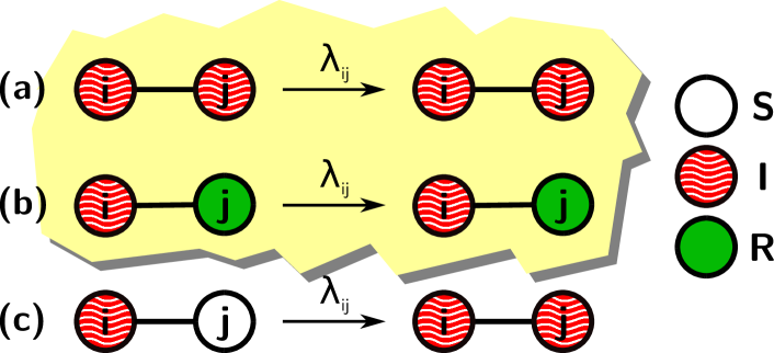
Figure 3: Examples of (a)-(b) phantom and (c) real infection processes for a pair o vertices $(i,j)$.

We write the total infection rate given by Eq. (20) as $L=W-P$ where

$$W=\sum_{i,j=1}^{N}\lambda_{ij}\delta(\sigma_{i},1)$$ (21)

is the total infection rate emanating from infected vertices, including the phantom processes, and

$$P=\sum_{i,j=1}^{N}\lambda_{ij}\delta(\sigma_{i},1)[\delta(\sigma_{j},1)+\delta(\sigma_{j},2)]$$ (22)

is the total infection attempts due to the phantom processes. The total rate of processes is $R=M+A+W$, which is larger than in GA since $W\geq L$.

We need now to calculate once at the beginning of and to keep stored along the simulation the maximal infection that can be produced by each vertex, given by

$$w_{i}=\sum_{j=1}^{N}\lambda_{ij}.$$ (23)

The general epidemic dynamics can be simulated as follows. We build and keep updated the lists $\mathcal{V}^{\text{(I)}}$, $\mathcal{M}$, $\mathcal{V}^{\text{(R)}}$, and $\mathcal{A}$ defined previously. We also need a list $\mathcal{W}$ with the infection $\mathcal{W}_{p}$ produced by the $p=1,\ldots,N_{\text{I}}$ infected vertices of the list $\mathcal{V}^{\text{(I)}}$, and the total infection rate

$$W=\sum_{p=1}^{N_{\text{I}}}\mathcal{W}_{p},$$ (24)

produced by these vertices. The update of $\mathcal{W}$ and $W$ follows the same steps of $\mathcal{M}$, $M$, $\mathcal{A}$, and $A$ described previously instead of the heavier task of building the list $\mathcal{V}^{\text{(IS)}}$ and calculating $L$ in the original GA. This point is essential for the algorithm efficiency as discussed in Sec. 6.

With probabilities $m=M/R$ and $a=A/R$ we perform, respectively, a recovering or waning of immunity as described for the original GA; cf. subsection 5.1. With probability $w=W/R$ an infected vertex is randomly selected as an element $p$ of $\mathcal{V}^{\text{(I)}}$ with probability proportional to $\mathcal{W}_{p}$ and let $i=\mathcal{V}^{\text{(I)}}_{p}$. Next, one neighbor $j$ of $i$ is chosen with probability proportional to $\lambda_{ij}$ using the rejection probability $\lambda_{ij}/\lambda_{i}^{(\text{max})}$, where $\lambda_{i}^{(\text{max})}=\max\limits_{j}\{\lambda_{ij}\}$. If the selected neighbor is susceptible, it is infected. If the selected neighbor is infected or recovered, i.e. a phantom process, no change of state is implemented, the time is incremented as in the original GA using $R=M+A+W$, and the simulation runs to the next time step. Note that the frustrated infection attempts reckon exactly the total rate of phantom processes $P$ given by Eq. (22). The values of $\lambda_{i}^{(\text{max})}$ need to be computed once at the beginning of the simulation. Depending on the model, further simplifications and improvements can be adopted.

5.3 Improved optimized Gillespie algorithm (IOGA)

We can improve the rejection method using smarter strategies to reduce the number of rejections with the cost of storing and updating more information. We call this method of improved optimized Gillespie algorithm (IOGA). For epidemic models on networks, the rates can be very heterogeneous as, for example, the total infection rates produced by vertices in the SIS model.

Let us consider the IOGA implementation for the infection processes using the simplest case with two lists for infected vertices. Define $w_{\text{max}}=\max\limits_{i}\{w_{i}\}$, cf. Eq. (23), and let $w_{*}$ be a threshold such that $w_{i}\leq w_{*}$ for the majority of vertices. We define two groups of vertices with $w_{i}\leq w_{*}$ and $w_{i}>w_{*}$. We build separated lists $\mathcal{V}^{\text{(I,low)}}$ and $\mathcal{V}^{\text{(I,high)}}$ with the $N_{\text{I}}^{\text{(low)}}$ and $N_{\text{I}}^{\text{(high)}}$ positions of the infected vertices, and also the lists of total infection rates $\mathcal{W}^{\text{(low)}}$ and $\mathcal{W}^{\text{(high)}}$, of vertices with $w_{i}\leq w_{*}$ and $w_{i}>w_{*}$, respectively. Then, we compute the total infection produced by each group $W^{(\text{low})}$ and $W^{(\text{high})}$. Note that $N_{\text{I}}=N_{\text{I}}^{\text{(low)}}+N_{\text{I}}^{\text{(high)}}$ and $W=W^{(\text{low})}+W^{(\text{high})}$. When an infection is selected to happen following the same rules as OGA, with probability $W^{(\text{low})}/W$ one element $p$ of $\mathcal{V}^{\text{(I,low)}}$ is chosen using a rejection probability $\mathcal{W}_{p}^{\text{(low)}}/w_{*}$ while, with probability $W^{(\text{high})}/W$, one element $p$ of $\mathcal{V}^{\text{(I,high)}}$ is chosen using a rejection probability $\mathcal{W}_{p}^{\text{(high)}}/w_{\text{max}}$. The generalization for healing and waning of immunity is straightforward. The time increment is the same as of OGA.

6 Application for specific epidemic models

6.1 SIS model

The implementation of the SIS model with states $\sigma_{i}=0$ or 1, rates $\mu_{i}=\mu$, $\alpha_{i}=\infty$, and $\lambda_{ij}=\lambda A_{ij}$ in the generic dynamics can be simplified considerably. Both GA and OGA for SIS do not need the list $\mathcal{M}$ since $\mathcal{M}_{p}=\mu$. The original GA reads as follows. The total healing and infection rates are $M=\mu N_{\text{I}}$ and $L=\lambda N_{\text{IS}}$, respectively, and $R=L+M$. With probability $m=M/R$ one infected vertex is chosen with equal chance ($\mu_{i}=\mu_{\text{max}}=\mu$) using $\mathcal{V}^{\text{(I)}}$ and healed (I$\rightarrow$S). With probability $l=L/R$, one element of the list $\mathcal{V}^{\text{(IS)}}$ is selected with equal chance ($\lambda_{ij}=\lambda_{\text{max}}=\lambda$) and the corresponding susceptible vertex is infected. The time, number of infected vertices, the list $\mathcal{V}^{\text{(I)}}$, number of IS edges and the list $\mathcal{V}^{\text{(IS)}}$ are updated.

We have that $\mathcal{W}_{p}=\lambda\mathcal{K}_{p}$, where $\mathcal{K}_{p}$ is the degree of the vertex stored in the $p$th entry of $\mathcal{V}^{\text{(I)}}$, is dispensable since if the vertex $i=\mathcal{V}^{\text{(I)}}_{p}$ is selected, its degree $\mathcal{K}_{p}=k_{i}$ is known. The total rates of healing and infection attempts, Eqs. (18) and (21), become $M=\mu N_{\text{I}}$ and $W=\lambda N_{\text{k}}$, respectively, where $N_{\text{k}}=\sum_{ij}A_{ij}\sigma_{i}=\sum_{i}k_{i}\sigma_{i}$ is the number of edges emanating from all infected vertices. Then, the total rate is $R=\mu N_{\text{I}}+\lambda N_{\text{k}}$. With probability $m=M/R$ an infected vertex $i$ is selected with equal chance using the list $\mathcal{V}^{\text{(I)}}$ and healed (I$\rightarrow$S). With probability $w=W/R$, an infected vertex $i$ is selected using $\mathcal{V}^{\text{(I)}}$ proportionally to its degree with a rejection probability $k_{i}/k_{\text{max}}$. The same infection rate for all edges implies that a neighbor of $i$ is chosen with equal chance and, if susceptible, it is infected. The time, number of infected vertices, edges emanating from them and the list $\mathcal{V}^{\text{(I)}}$ are updated.

The probability $k_{i}/k_{\text{max}}$ of the OGA for SIS implies in too many rejections for power-law degree distributions. The fraction of vertices with degree less than $k_{*}$ is approximately given by

$$\sum\limits_{k=k_{0}}^{k_{*}}P(k)\simeq\left[1-\left(\frac{k_{0}}{k_{*}}\right)^{\gamma-1}\right].$$ (25)

The optimal choice of $k_{*}$ will depend on the degree distribution. To be effective, $k_{*}$ should not be much larger than the degree of the wide majority of vertices and thus the result of Eq. (25) must not be far from 1. For IOGA simulations presented here, $k_{*}=2\langle{k}\rangle$ was used.

The IOGA implementation for SIS is the following. The infected vertex to be healed is chosen at random from either the lists $\mathcal{V}^{\text{(I,low)}}$ or $\mathcal{V}^{\text{(I,high)}}$ with probabilities $N_{\text{I}}^{\text{(low)}}/N_{\text{I}}$ or $N_{\text{I}}^{\text{(high)}}/N_{\text{I}}$, respectively, since $M^{\text{(low)}}=\mu N_{\text{I}}^{\text{(low)}}$ and $M^{\text{(high)}}=\mu N_{\text{I}}^{\text{(high)}}$. In the infection event, with probabilities $N_{\text{k}}^{\text{(low)}}/N_{\text{k}}$ or $N_{\text{k}}^{\text{(high)}}/N_{\text{k}}$, one vertex $i$ is selected from $\mathcal{V}^{\text{(I,low)}}$ or $\mathcal{V}^{\text{(I,high)}}$ using the rejection probabilities $k_{i}/k_{*}$ or $k_{i}/k_{\text{max}}$, respectively. The time, number of infected vertices in each compartment ($N_{\text{I}}^{\text{(low)}}$ and $N_{\text{I}}^{\text{(high)}}$), edges emanating from them ($N_{\text{k}}^{\text{(low)}}$ and $N_{\text{k}}^{\text{(high)}}$) and the lists ($\mathcal{V}^{\text{(I,low)}}$ and $\mathcal{V}^{\text{(I,low)}}$) are updated.

Typical outcomes of different algorithms for SIS simulations are compared in Fig. 4 for a single realization of a same UCM network with exponent $\gamma=4.0$, $N=10^{4}$ and cutoff $k_{c}\sim N^{1/\gamma}$. In the main plot, we show the density of infected vertices against time using standard averaging (samples that visited absorbing states before time $t$ are reckoned) over many independent runs with initial condition $\rho(0)=1$. In the inset, the QS density against infection rate is shown. Differences between curves are noticeable only for very low densities due to the finite number of samples. Excellent matches are also obtained for the QS probability distribution, a benchmark of the dynamics, of SIS epidemics at the threshold as shown in Fig. 5. Tiny differences due to finite statistics are present for very low probabilities. Essentially perfect matches of the QS distributions are also found in both super and subcritical phases. Fortran and Python codes for the decay simulations are available in [34]. The former was tested for GNU [44] and Intel [45] non-commercial Linux versions of Fortran and the latter using Python 3.6.0 [46].

Here, it is worth to mention that the average time step given by $\langle{\tau}\rangle=1/R$ is commonly used as the time increment [8, 10, 11, 12, 13, 16, 32, 33] instead of drawing it according to an exponential distribution given by Eq. (16). We verified that this step of the implementation is irrelevant for both QS analysis and decay simulations with large averaging and thus these previously obtained results are computationally valid.

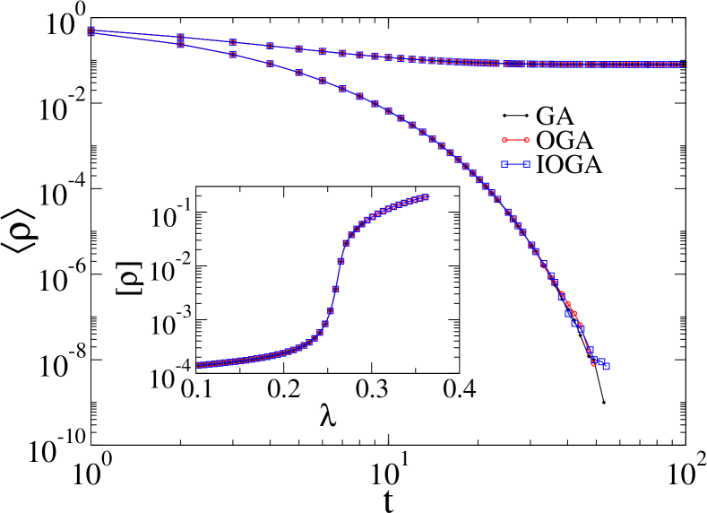
Figure 4: Density against time for SIS model with $\mu=1$ on a single network realization of the UCM model with $\gamma=4.0$, $k_{0}=3$, $N=10^{4}$, and $k_{c}\sim N^{1/\gamma}$. The infection rates are $\lambda=0.150<\lambda_{c}$ (bottom curves) and $\lambda=0.300>\lambda_{c}$ (top curves). The averages were done over $10^{5}$ and $10^{4}$ independent runs below and above the epidemic threshold with initial condition $\rho(0)=1$. Inset shows the QS density against infection rate.

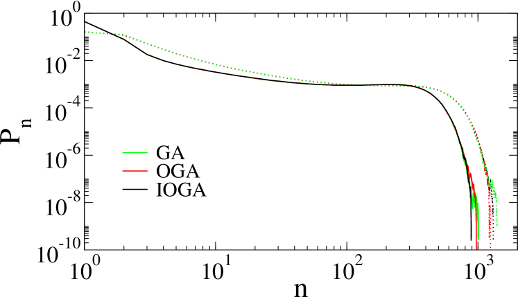
Figure 5: Quasistationary probability distribution for SIS model at the epidemic threshold estimated via susceptibility (see Table 1) with $\mu=1$ on UCM networks using distinct algorithms. The network parameters are $N=10^{5}$, $k_{0}=3$, $k_{c}\sim N^{1/\gamma}$, $\gamma=2.3$ (solid lines) and $\gamma=4.0$ (dotted lines).

We compared the CPU times performing QS simulations at and above the epidemic threshold estimated via the maxima of the susceptibility for $\mu=1$; see Table 1 for the threshold values used in the simulations. We started with 1% of infected vertices and ran the dynamics during $t_{\text{av}}+t_{\text{rlx}}=3\times 10^{6}$. Networks with different levels of heterogeneity were investigated: weakly heterogeneous networks with degree given by $k=k_{0}+k^{\prime}$, where $k_{0}=3$ is fixed and $k^{\prime}$ is drawn from an exponential distribution $P(k^{\prime})=a\exp(-k^{\prime}/a)$ with $a=3$ and $k^{\prime}\geq 0$; UCM networks with either $\gamma=2.3$ and $4.0$, $k_{c}\sim N^{1/\gamma}$ and minimal degree $k_{0}=3$. All CPU time comparisons were performed in a workstation with two six-core Intel Xeon processors E5-2620 2.00 GHz and 32 Gb of RAM memory. The code was written in Fortran and compiled with a non-commercial version of the Intel Fortran for Linux 64-bit using double precision and standard compilation optimizations.

$N$	SIS			CP
	Exp.	$\gamma=2.3$	$\gamma=4.0$	$\gamma=2.3$	$\gamma=4.0$
$1\times 10^{3}$	$0.1705$	$0.1065$	$0.3113$	$1.2606$	$1.4691$
$3\times 10^{3}$	$0.1674$	$0.0749$	$0.2912$	$1.2181$	$1.4338$
$1\times 10^{4}$	$0.1614$	$0.0524$	$0.2619$	$1.1807$	$1.4058$
$3\times 10^{4}$	$0.1605$	$0.0393$	$0.2515$	$1.1626$	$1.3950$
$1\times 10^{5}$	$0.1603$	$0.0280$	$0.2319$	$1.1445$	$1.3872$
$3\times 10^{5}$	$0.1602$	$0.0198$	$0.2254$	$1.1335$	$1.3855$
$1\times 10^{6}$	$0.1593$	$0.0141$	$0.2166$	$1.1255$	$1.3830$
$3\times 10^{6}$	$0.1592$	$0.0104$	$0.2065$	$1.1197$	$1.3813$
$1\times 10^{7}$	$0.1591$	$0.0073$	$0.1956$	$1.1145$	$1.3807$

Table 1: Threshold values used in the simulations of SIS and CP dynamics with $\mu=1$ for networks with different levels of heterogeneity, estimated via susceptibility.

CPU times for the SIS at the epidemic threshold as a function of the network size are compared in Fig. 6 and Table 2. The CPU time for GA increases almost linearly while for OGA and IOGA it does sublinearly. The relative gain of IOGA in comparison with OGA is appreciable even in networks without outliers as can be seen in Table 2.

Figure 6: CPU times for QS simulations of the SIS dynamics at the epidemic threshold (see Table 1) for networks with different levels of heterogeneities: (a) Exponential; (b) UCM with $\gamma=2.3$; (c) UCM with $\gamma=4.0$; and (d) UCM with $\gamma=4.0$ plus an outlier (see main text). The total simulation time is $t_{\text{av}}+t_{r}=3\times 10^{6}$. Solid and dashed lines are guides to the eyes.

	GA		OGA			IOGA
$N$	$10^{5}$	$10^{6}$	$10^{5}$	$10^{6}$	$10^{7}$	$10^{5}$	$10^{6}$	$10^{7}$
Exp.	379	4970	3.55	11.6	36.9	2.73	10.8	33.7
$\gamma=2.3$	255	3540	1.50	4.86	11.3	1.15	3.48	8.27
$\gamma=4.0$	153	2010	3.34	8.99	25.7	2.14	7.09	15.4
Outlier	2630	—	33.8	147	536	14.3	46.6	136

Table 2: CPU times in minutes for QS simulations of the SIS model at the epidemic threshold in networks of different sizes and levels of heterogeneity using different simulation methods. The total simulation time is $t_{\text{av}}+t_{r}=3\times 10^{6}$ steps.

To investigate the role of outliers in the computer efficiency we considered the UCM network with $k_{c}\sim N^{1/\gamma}$ adding a vertex with degree $k_{\text{out}}\gg k_{c}$. We chose $k_{\text{out}}=\langle{k_{\text{max}}}\rangle$ where $\langle{k_{\text{max}}}\rangle$ is the mean value of the maximal degree obtained in network with cutoff $k_{c}=N$. The presence of this outlier leads to a metastable and localized phase in SIS dynamics: see also Refs. [13, 31, 32]. We performed simulations for $\gamma=4.0$ at the epidemic threshold determined for the network without the outlier, shown in Table 1. The system having an outlier remains critical with density of infected vertices decaying as $\rho_{\text{out}}\approx 20N^{-0.67}$, which is much larger than the density obtained without the outlier given by $\rho\approx 3.4N^{-0.67}$. Figure 6(d) shows the CPU times obtained for simulations with the outlier using different methods. The computational gain of IOGA in relation to OGA is very expressive and becomes more relevant as the network size increases as can be also seen in Table 2.

Above the epidemic threshold all simulations becomes much slower than the critical ones. We compared the efficiencies for a UCM network with $\gamma=2.3$ and $k_{c}\sim N^{1/\gamma}$ at an infection rate $\lambda=\lambda_{c}+0.02$ and $\mu=1$. The CPU time increases linearly with size for OGA and IOGA and no significant difference between them was observed in the absence of outliers. The GA simulations becomes exceedingly slow with CPU times scaling as $t_{\text{CPU}}\sim N^{1.6}$. For example, the QS simulation in networks with $N=10^{4}$ and $t_{\text{av}}+t_{r}=3\times 10^{6}$ takes approximately 2.5 days for GA against 10 min for OGA or IOGA.

The slowness of GA is due to the building of the lists after every state change, for which we have to visit all neighbors of a finite fraction of the network. The linear increase of the simulation times for the optimized algorithms is reflecting that the amount of independent events is proportional to the number of infected vertices. Note that if the analysis is not done close to the epidemic threshold, relatively small systems are sufficient to obtain the behavior of the thermodynamical limit and OGA will be sufficient to this job.

6.2 Contact process

The contact process (CP) [8, 16, 20] is obtained from the generic epidemic dynamics with $\mu_{i}=\mu$, $\alpha_{i}=\infty$, and $\lambda_{ij}=\lambda A_{ij}/k_{i}$. This subtle modification in the infection rate leads to differences with SIS model that becomes remarkable in networks with PL degree distributions. A central one is that the total infection rate produced by a vertex in CP is independent of its degree and given by $w_{i}=\lambda$ in contrast with $w_{i}=\lambda k_{i}$ for SIS, see Eq. (23), that leads to a finite epidemic threshold for CP for any value of the degree exponent $\gamma$ [16, 19, 20].

The total rate of healing is the same of the SIS, given by $M=\mu N_{\text{I}}$. The GA algorithm for CP follows the same steps of SIS implementation to build the lists $\mathcal{V}^{\text{(I)}}$ and $\mathcal{V}^{\text{(IS)}}$. Instead of $\mathcal{L}$, a list $\mathcal{K}$ with the degree $\mathcal{K}_{p}$ of the $p=1,\ldots,N_{\text{IS}}$ infected vertices connected to each susceptible vertex recorded at $\mathcal{V}^{\text{(IS)}}$ and the total infection rate transmitted along IS edges

$$L=\lambda\sum_{i,j=1}^{N}\frac{A_{ij}}{k_{i}}\sigma_{i}(1-\sigma_{j})=\sum_{p=1}^{N_{\text{IS}}}\frac{\lambda}{\mathcal{K}_{p}}$$ (26)

are computed. Note that $\mathcal{L}_{p}=\lambda/\mathcal{K}_{p}$. The total rate is $R=M+L$. With probability $m=M/R$ an infected vertex is chosen with equal chance using the auxiliary list $\mathcal{V}^{\text{(I)}}$ and healed. With probability $l=L/R$ one susceptible vertex is chosen as an element $p$ of $\mathcal{V}^{\text{(IS)}}$ applying a rejection probability $k_{\text{min}}/\mathcal{K}_{p}$ since $\lambda_{\text{max}}=\lambda/k_{\text{min}}$. The time is incremented, and the lists $N_{\text{I}}$ and $\mathcal{V}^{\text{(I)}}$ are updated as in the SIS algorithm.

For OGA, the total infection rate including the phantom processes is $W=\lambda N_{\text{I}}$. Since $w_{i}=\lambda$ and $\lambda_{ij}=\lambda/k_{i}$ is independent of the target $j$, the acceptance probabilities of both chosen vertex and target neighbor become 1 and we obtain the widely used recipe for CP simulation [8, 16]: An infected vertex $i$ is selected with equal chance using the list $\mathcal{V}^{\text{(I)}}$. With probability $m=M/R=\mu/(\mu+\lambda)$ the selected vertex is healed. With probability $w=W/R=\lambda/(\mu+\lambda)$, one of the $k_{i}$ neighbors of $i$ is randomly selected and, if susceptible, is infected. Otherwise no change of state is implemented. The time is incremented, $N_{\text{I}}$ and $\mathcal{V}^{\text{(I)}}$ are updated as in the SIS algorithm.

Since the rejection method is not used in OGA, IOGA losses its sense for CP.

The equivalence between GA and OGA algorithms for CP is shown in Fig. 7 for both decay and QS simulations. As in SIS, the curves are distinguishable only at very low values due to finite statistics. The computational times for both algorithms are compared in Fig. 8 where we see that the critical dynamics (see Table 1 for thresholds) can be several orders of magnitude slower in the non-optimized algorithm and the difference increases with the network size. As in SIS, the differences become larger above the epidemic threshold.

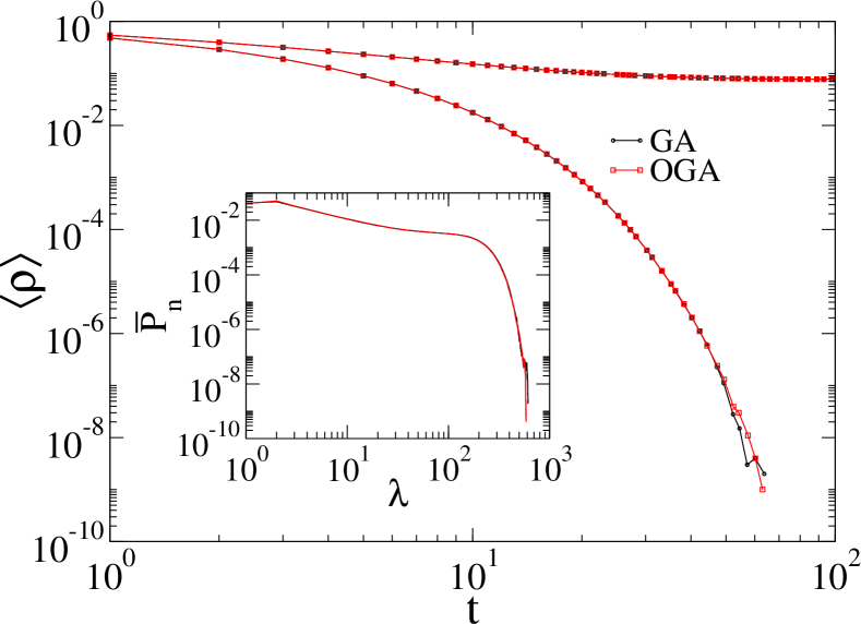
Figure 7: Comparison of algorithms for CP with $\mu=1$ on an UCM network with $\gamma=4.0$, $N=10^{4}$, $k_{0}=3$, $k_{c}\sim N^{1/\gamma}$ using infection rates $\lambda=0.9<\lambda_{c}$ (bottom curves) and $\lambda=1.5>\lambda_{c}$ (top curves). The averages were performed over $10^{5}$ and $10^{4}$ samples for $\lambda<\lambda_{c}$ and $\lambda>\lambda_{c}$, respectively. Inset shows the QS distribution for CP dynamics at the epidemic threshold (see Table 1) on a UCM network with the same parameters of the main plot.

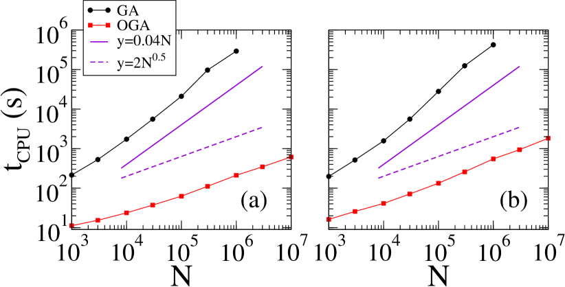
Figure 8: Comparison of CPU times for QS simulations of the CP with $\mu=1$ using two algorithms. The simulations were performed at the epidemic threshold (see Table 1) on UCM networks with minimal degree $k_{0}=3$, $k_{c}\sim N^{1/\gamma}$ and degree exponents (a) $\gamma=2.3$ and (b) $\gamma=4.0$. The total simulation time is $t_{\text{av}}+t_{r}=3\times 10^{6}$. Lines are guides to the eyes.

6.3 SIR model

Choosing $\mu_{i}=\mu$, $\alpha_{i}=0$, and $\lambda_{ij}=\lambda A_{ij}$ for all vertices, one obtains the SIR model [43]. Differently from SIS and CP, SIR does not have an active stationary state. The implementation of SIR is very similar to SIS with the difference that the transition I$\rightarrow$S is changed to I$\rightarrow$R, and vertices in state R do not change in this model.

We performed SIR simulations starting with a single infected vertex and the remaining of the network susceptible. To reduce fluctuations we always start in the most connected vertex of the network. The simulation proceeds until an absorbing state is reached and the averages were performed over $10^{5}$ repetitions in the same network. The list of recovered vertices $\mathcal{V}^{\text{(R)}}$ is not necessary for this dynamical simulation since the recovered vertices do not have dynamics. However, it can be useful to keep this list updated and use it to setup the initial condition efficiently visiting only the recovered vertices and resetting them to the susceptible state. A gain of up to one order of magnitude can be obtained with this procedure since many samples do not lead to large outbreaks, specially near and below the epidemic threshold. Thus, after an outbreak, only a few vertices have to be updated to reset the initial condition.

We calculated the final density of recovered vertices and the average time that the activity in the epidemic outbreak lasts. The equivalence between algorithms for SIR is shown in Fig. 9 for a UCM network with $\gamma=4.0$. Other degree exponents were considered and the equivalence corroborated. The time dependence of the average number of infected and recovered vertices are also indistinguishable when the three algorithms are used. The comparative computer efficiency of SIR algorithms is similar to SIS.

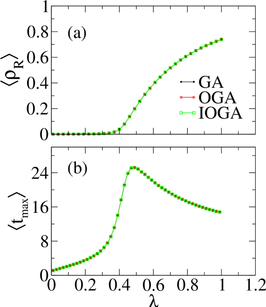
Figure 9: Comparison of the SIR dynamics with different algorithms in a UCM network with degree exponent $\gamma=4.0$ and $N=10^{4}$ vertices, $k_{0}=3$ and $k_{c}\sim N^{1/\gamma}$. The final (a) average density of recovered vertices and (b) epidemic lifetime are shown as a function of the infection rate. The curves correspond to average over $10^{5}$ samples.

6.4 Algorithms for more complicated dynamics

We now provide two others examples of the OGA implementation. For $\mu_{i}=\mu$, $\alpha_{i}=\alpha$, and $\lambda_{ij}=\lambda A_{ij}$ we have the classic susceptible-infected-recovered-susceptible (SIRS) [43] model and the algorithm described in Ref. [15] as follows. The lists $\mathcal{V}^{\text{(I)}}$ and $\mathcal{V}^{\text{(R)}}$ and the variables $N_{\text{R}}$, $N_{\text{I}}$, and $N_{\text{k}}$ (cf. SIS algorithm for OGA) are computed and constantly updated. The total healing, waning of immunity and infection attempt rates are $M=\mu N_{\text{I}}$, $A=\alpha N_{\text{R}}$, and $W=\lambda N_{\text{k}}$, respectively, with a total rate $R=M+A+W$. With probability $m=M/R$ one infected vertex is selected at random using $\mathcal{V}^{\text{(I)}}$ and healed. With probability $a=A/R$, a recovered vertex is selected at random using $\mathcal{V}^{\text{(R)}}$ and converted to susceptible. Finally, with probability $w=W/R$, an infection attempt is performed in two steps: An infected vertex $j$ is selected with probability proportional to its degree. A neighbor of $j$ is selected with equal chance and, if susceptible, it is infected. The other steps are the same of SIS.

The generalized SIS model with $\mu_{i}=\mu$, $\alpha_{i}=\infty$ and $\lambda_{ij}=\lambda A_{ij}/(k_{i}k_{j})^{\theta}$, where $\theta$ is a model parameter, was proposed and investigated by Karsai, Juhász, and Iglói (KJI) [47]. We can derive the implementation of the KJI model presented in Ref. [15] generalizing the SIS algorithm using Eqs. (21) and (23) as follows. The lists $\mathcal{V}^{\text{(I)}}$ and $\mathcal{W}$ and the variables $N_{\text{I}}$ and $W$, Eq. (24), are computed and constantly updated. The total healing rate is $M=\mu N_{\text{I}}$ and the total rate is $R=M+W$. With probability $m=M/R$ one infected vertex is selected at random using $\mathcal{V}^{\text{(I)}}$ and becomes susceptible. With probability $w=W/R$, a vertex $i$ is chosen as an element $p$ of $\mathcal{V}^{\text{(I)}}$ using a rejection probability $\mathcal{W}_{p}/w_{\text{max}}$. Next, a neighbor of $i=\mathcal{V}^{\text{(I)}}_{p}$, namely $j$, is selected using a rejection probability $\left[k_{i}^{\text{(min)}}/k_{j}\right]^{\theta}$ where $k_{i}^{\text{(min)}}$ is the smallest degree among the neighbors of $i$. If $j$ is susceptible, it becomes infected. Other steps are the same of SIS.

7 Concluding remarks

In the present work, we show how to build statistically exact algorithms for simulations of generic epidemic processes on very large and heterogeneous networked systems. Grounded in the classical Gillespie algorithm [21, 22] for simulation of stochastic processes, we developed optimized versions of the GA by introducing the idea of phantom processes that are transitions that do not lead to changes of states but do count for time increments. These phantom processes simplify hugely the determination of the all possible events and the optimized Gillespie algorithms can be several orders of magnitude more efficient that the original one but still providing statistically exactly simulations. We provide comparisons for the equivalence among the methods and compared their computer efficiencies for basic epidemic models, namely, the SIS, contact processes, and SIR models.

The original GA is much slower than OGA due to the building of the lists of all possible events after every change of state, for which is necessary to check all neighbors of each infected vertex. We could roughly estimate the number of operations per time step of GA as of order $N_{\text{I}}\langle{k}\rangle$ while in OGA it is approximately constant. The number of operations by time unity is inversely proportional to the average time step and simulation CPU time will increase with $N_{\text{I}}$ as well. So, the optimized algorithms we investigated constitute great optimizations when the density of infected vertices is low, which is particularly relevant for analyses close to the epidemic threshold.

Searching in the literature, one can find implementations of continuous-time epidemic models that are not statistically exact [28, 48, 49]. So, it would be interesting to check the impact of these modified implementations on the final outcome comparing them with the statistically exact prescriptions described in this work. The ideas developed here can be used as a groundwork for the building of efficient algorithms for other Markovian dynamical process and also for building optimizations for breakthrough topics on network theory involving non-Markovian epidemic processes [24, 50] and temporal networks [51].

References

References

- [1] M. Newman, Networks: An Introduction, Oxford University Press, Inc., New York, NY, USA, 2010.
- [2] A. Barabási, Network Science, Cambridge University Press, 2016.
- [3] P. Sen, B. Chakrabarti, Sociophysics: An Introduction, OUP Oxford, 2013.
- [4] L. da F. Costa, O. N. Oliveira, G. Travieso, F. A. Rodrigues, P. R. Villas Boas, L. Antiqueira, M. P. Viana, L. E. Correa Rocha, Analyzing and modeling real-world phenomena with complex networks: a survey of applications, Adv. Phys. 60 (3) (2011) 329–412.
- [5] A. Barrat, M. Barthélemy, A. Vespignani, Dynamical Processes on Complex Networks, Cambridge University Press, Cambridge, UK New York, 2012.
- [6] R. Pastor-Satorras, C. Castellano, P. Van Mieghem, A. Vespignani, Epidemic processes in complex networks, Rev. Mod. Phys. 87 (3) (2015) 925–979.
- [7] S. N. Dorogovtsev, A. V. Goltsev, J. F. F. Mendes, Critical phenomena in complex networks, Rev. Mod. Phys. 80 (2008) 1275–1335.
- [8] J. Marro, R. Dickman, Nonequilibrium phase transitions in lattice models, Collection Alea-Saclay: Monographs and Texts in Statistical Physics, Cambridge University Press, Cambridge, 2005.
- [9] C. Castellano, R. Pastor-Satorras, Thresholds for epidemic spreading in networks, Phys. Rev. Lett. 105 (2010) 218701.
- [10] S. C. Ferreira, C. Castellano, R. Pastor-Satorras, Epidemic thresholds of the susceptible-infected-susceptible model on networks: A comparison of numerical and theoretical results, Phys. Rev. E 86 (2012) 041125.
- [11] H. K. Lee, P.-S. Shim, J. D. Noh, Epidemic threshold of the susceptible-infected-susceptible model on complex networks, Phys. Rev. E 87 (2013) 062812.
- [12] M. Boguñá, C. Castellano, R. Pastor-Satorras, Nature of the epidemic threshold for the susceptible-infected-susceptible dynamics in networks, Phys. Rev. Lett. 111 (2013) 068701.
- [13] A. S. Mata, S. C. Ferreira, Multiple transitions of the susceptible-infected-susceptible epidemic model on complex networks, Phys. Rev. E 91 (2015) 012816.
- [14] P. Shu, W. Wang, M. Tang, Y. Do, Numerical identification of epidemic thresholds for susceptible-infected-recovered model on finite-size networks, Chaos 25 (6).
- [15] S. C. Ferreira, R. S. Sander, R. Pastor-Satorras, Collective versus hub activation of epidemic phases on networks, Phys. Rev. E 93 (2016) 032314.
- [16] C. Castellano, R. Pastor-Satorras, Non-mean-field behavior of the contact process on scale-free networks, Phys. Rev. Lett. 96 (2006) 038701.
- [17] H. Hong, M. Ha, H. Park, Finite-Size Scaling in Complex Networks, Phys. Rev. Lett. 98 (25) (2007) 258701.
- [18] C. Castellano, R. Pastor-Satorras, Routes to thermodynamic limit on scale-free networks, Phys. Rev. Lett. 100 (2008) 148701.
- [19] S. C. Ferreira, R. S. Ferreira, C. Castellano, R. Pastor-Satorras, Quasistationary simulations of the contact process on quenched networks, Phys. Rev. E 84 (2011) 066102.
- [20] A. S. Mata, R. S. Ferreira, S. C. Ferreira, Heterogeneous pair-approximation for the contact process on complex networks, New J. Phys. 16 (2014) 053006.
- [21] D. T. Gillespie, A general method for numerically simulating the stochastic time evolution of coupled chemical reactions, J. Comput. Phys. 22 (4) (1976) 403–434.
- [22] D. T. Gillespie, Exact stochastic simulation of coupled chemical reactions, J. Phys. Chem. 81 (25) (1977) 2340–2361.
- [23] P. G. Fennell, S. Melnik, J. P. Gleeson, Limitations of discrete-time approaches to continuous-time contagion dynamics, Phys. Rev. E 94 (5) (2016) 052125.
- [24] M. Boguñá, L. F. Lafuerza, R. Toral, M. A. Serrano, Simulating non-markovian stochastic processes, Phys. Rev. E 90 (2014) 042108.
- [25] R. Pastor-Satorras, A. Vespignani, Epidemic spreading in scale-free networks, Phys. Rev. Lett. 86 (2001) 3200–3203.
- [26] S. Gómez, A. Arenas, J. Borge-Holthoefer, S. Meloni, Y. Moreno, Discrete-time markov chain approach to contact-based disease spreading in complex networks, EPL 89 (2010) 38009.
- [27] D. Chakrabarti, Y. Wang, C. Wang, J. Leskovec, C. Faloutsos, Epidemic thresholds in real networks, ACM Trans. Inf. Syst. Secur. 10 (2008) 1–26.
- [28] V. M. Eguíluz, K. Klemm, Epidemic threshold in structured scale-free networks, Phys. Rev. Lett. 89 (2002) 108701.
- [29] P. Shu, W. Wang, M. Tang, P. Zhao, Y.-C. Zhang, Recovery rate affects the effective epidemic threshold with synchronous updating, Chaos 26 (2016) 063108.
- [30] A. S. Mata, S. C. Ferreira, Pair quenched mean-field theory for the susceptible-infected-susceptible model on complex networks, EPL 103 (4) (2013) 48003.
- [31] W. Cota, S. C. Ferreira, G. Ódor, Griffiths effects of the susceptible-infected-susceptible epidemic model on random power-law networks, Phys. Rev. E 93 (3) (2016) 032322.
- [32] G. F. de Arruda, E. Cozzo, T. P. Peixoto, F. A. Rodrigues, Y. Moreno, Disease Localization in Multilayer Networks, Phys. Rev. X 7 (1) (2017) 011014.
- [33] G. St-Onge, J.-G. Young, E. Laurence, C. Murphy, L. J. Dubé, Susceptible-infected-susceptible dynamics on the rewired configuration model. arXiv:1701.01740.
- [34] The codes are freely available at https://github.com/wcota/dynSIS.
- [35] M. Molloy, B. Reed, A critical point for random graphs with a given degree sequence, Random Struct. Algor. 6 (2-3) (1995) 161–180.
- [36] W. H. Press, S. A. Teukolsky, W. T. Vetterling, B. P. Flannery, Numerical Recipes 3rd Edition: The Art of Scientific Computing, 3rd Edition, Cambridge University Press, New York, NY, USA, 2007.
- [37] M. Boguñá, R. Pastor-Satorras, A. Vespignani, Cut-offs and finite size effects in scale-free networks, Eur. Phys. J. B 38 (2004) 205–210.
- [38] M. Boguñá, C. Castellano, R. Pastor-Satorras, Langevin approach for the dynamics of the contact process on annealed scale-free networks, Phys. Rev. E 79 (3) (2009) 036110.
- [39] M. Catanzaro, M. Boguñá, R. Pastor-Satorras, Generation of uncorrelated random scale-free networks, Phys. Rev. E 71 (2005) 027103.
- [40] R. Pastor-Satorras, A. Vespignani, Evolution and Structure of the Internet: A Statistical Physics Approach, Cambridge University Press, 2007.
- [41] N. van Kampen, Stochastic Processes in Physics and Chemistry, North-Holland Personal Library, Elsevier Science, 2011.
- [42] R. S. Sander, G. S. Costa, S. C. Ferreira, Sampling methods for the quasistationary regime of epidemic processes on regular and complex networks, Phys. Rev. E 94 (4) (2016) 042308.
- [43] R. Anderson, R. May, Infectious Diseases of Humans: Dynamics and Control, Dynamics and Control, OUP Oxford, 1992.
- [44] See https://gcc.gnu.org/fortran/.
- [45] See https://software.intel.com/en-us/fortran-compilers.
- [46] See https://www.python.org/downloads/release/python-360/.
- [47] M. Karsai, R. Juhász, F. Iglói, Nonequilibrium phase transitions and finite-size scaling in weighted scale-free networks, Phys. Rev. E 73 (2006) 036116.
- [48] R. Pastor-Satorras, A. Vespignani, Epidemic dynamics and endemic states in complex networks, Phys. Rev. E 63 (2001) 066117.
- [49] G. Ódor, Spectral analysis and slow spreading dynamics on complex networks, Phys. Rev. E 88 (3) (2013) 032109.
- [50] I. Z. Kiss, G. Röst, Z. Vizi, Generalization of pairwise models to non-markovian epidemics on networks, Phys. Rev. Lett. 115 (2015) 078701.
- [51] C. L. Vestergaard, M. Génois, Temporal Gillespie Algorithm: Fast Simulation of Contagion Processes on Time-Varying Networks, PLOS Comp. Bio. 11 (10) (2015) e1004579.