Turbulence in three-dimensional simulations of magnetopause reconnection

Abstract

We present detailed analysis of the turbulence observed in three-dimensional particle-in-cell simulations of magnetic reconnection at the magnetopause. The parameters are representative of an electron diffusion region encounter of the Magnetospheric Multiscale (MMS) mission. The turbulence is found to develop around both the magnetic X line and separatrices, is electromagnetic in nature, is characterized by a wave vector $k$ given by $k\rho_{e}\sim(m_{e}T_{e}/m_{i}T_{i})^{0.25}$ with $\rho_{e}$ the electron Larmor radius, and appears to have the ion pressure gradient as its source of free energy. Taken together, these results suggest the instability is a variant of the lower hybrid drift instability. The turbulence produces electric field fluctuations in the out-of-plane direction (the direction of the reconnection electric field) with an amplitude of around $\pm 10$ mV/m, which is much greater than the reconnection electric field of around $0.1$ mV/m. Such large values of the out-of-plane electric field have been identified in the MMS data. The turbulence in the simulations controls the scale lengths of the density profile and current layers in asymmetric reconnection, driving them closer to $\sqrt{\rho_{e}\rho_{i}}$ than the $\rho_{e}$ or $d_{e}$ scalings seen in 2-D reconnection simulations, and produces significant anomalous resistivity and viscosity in the electron diffusion region.

I Introduction

During magnetic reconnection topological changes in the magnetic field trigger the transfer of magnetic energy to the surrounding plasma, where it appears as flows, thermal energy, and nonthermal particles. The change of topology occurs at magnetic X lines, which are embedded within electron diffusion regions. The recently launched Magnetospheric Multiscale (MMS) mission is designed to make high-resolution spatial and temporal measurements within electron diffusion regions and explore the small-scale activity, including turbulence, found there (Burch et al., 2016).

The initial phase of the MMS mission focused on the magnetopause, the location where the plasmas of the magnetosheath and magnetosphere reconnect. Such reconnection is typically asymmetric (Cassak and Shay, 2007) and includes significant differences between the magnetic fields, densities, and ion and electron temperatures. The strong gradients across the magnetopause associated with these asymmetries are susceptible to the generation of drift waves and their associated instabilities. Of particular interest for reconnection, which produces ambient gradients with scale lengths at or below the ion Larmor radius $\rho_{i}$ or ion inertial scale $d_{i}$, is the lower hybrid drift instability (LHDI). The theory of this instability has been widely explored in previous work (Davidson and Gladd, 1975; Daughton, 2003; Huba et al., 1982; Roytershteyn et al., 2012; Winske, 1981; Yoon et al., 2008).

The fundamental energy sources for LHDI are magnetic field and plasma pressure inhomogeneities that drive the relative drifts of electrons and ions. In the case of the magnetopause the relative drift of the electrons and protons arises dominantly from the ${E}\times{B}$ drift of electrons: the ion pressure across the magnetopause is to lowest order balanced by a Hall electric field

$$E_{x}\sim\frac{1}{ne}\frac{\partial P_{i}}{\partial x}\sim\frac{P_{i}}{neL_{i}}$$ (1)

with $P_{i}$ the ion pressure and $L_{i}$ the ion pressure scale length (we use GSM coordinates with $x$ pointing toward the sun, $y$ pointing in the azimuthal direction and $z$ pointing to the north). The consequence is that to lowest order the net ion drift in the $y$ direction is zero because the ${E}\times{B}$ and diamagnetic drifts cancel. The Hall electric field drives a current of electrons

$$v_{de}\sim\frac{cE_{x}}{B_{z}}\sim\frac{cT_{i}}{eB_{z}L_{i}}\sim v_{*i}$$ (2)

in the $y$ direction that is equal in magnitude to the ion diamagnetic velocity $v_{*i}=v_{i}\rho_{i}/L_{i}$. This strong drift is reflected in the crescent-shaped electron velocity distributions documented in MMS observations (Burch et al., 2016). Because $T_{i}\gg T_{e}$ at the magnetopause, electron diamagnetic drifts are small compared with this ${E}\times{B}$ drift. Thus, it is fundamentally the ion pressure gradient that is the driver of the relative drift of ions and electrons and the driver of drift-type instabilities. (This statement can be cast in a different form by noting that the ion-pressure-driven drifts and associated currents support the reversal in the direction of the magnetic field across the magnetopause. Since the system is inductive, the integral of the current across the reversal is an invariant and the magnetic free energy, which must be related to the pressure, can be considered the effective energy source.)

Regardless of the physical description, the basic characteristics of the LHDI in the low-$\beta$ “local approximation” (for which the profiles of pressure and current are neglected) are electrostatic oscillations, ${k}\bm{\cdot}{B}=0$, a most unstable mode satisfying $k\rho_{e}\sim 1$, and $\omega\sim kv_{*i}\lesssim\Omega_{\text{lh}}$. Here $\omega$ is the mode frequency, $k$ is the wave number, $\rho_{e}$ is the electron Larmor radius and $\Omega_{\text{lh}}=\sqrt{\omega_{ce}\omega_{ci}}$ is the lower hybrid frequency.

However, these properties are modified when the LHDI is excited in a narrow current sheet (one with a width of order the ion gyroradius or smaller). Theory and simulations (Winske, 1981; Daughton, 2003) suggest that the “local” mode described above quickly saturates and another longer-wavelength instability subsequently develops. The new LHDI mode is electromagnetic and has a wave number $k\rho_{e}\sim(m_{e}T_{e}/m_{i}T_{i})^{0.25}$. In addition, while the shorter wavelength electrostatic fluctuations tend to be confined to the edges of the current sheet (being stabilized at high $\beta=8\pi P/B^{2}$), the longer wavelength electromagnetic mode penetrates to the sheet’s center. Moreover, the electromagnetic mode need not strictly satisfy ${k}\bm{\cdot}{B}=0$. In light of this longer wavelength mode, LHDI is expected to satisfy somewhat more relaxed conditions: $(m_{e}T_{e}/m_{i}T_{i})^{0.25}\leq k\rho_{e}\leq 1$ and $\omega_{\text{ci}}\leq\omega\leq\Omega_{\text{lh}}$.

In a previous paper (Price et al., 2016) we performed a three-dimensional simulation of reconnection with initial conditions representative of an MMS observation of an electron diffusion region (Burch et al., 2016). As part of that work we observed turbulence developing around both the X line and the separatrices. We suggested that the turbulence was due to LHDI. These conclusions were consistent with earlier magnetopause observations (Bale et al., 2002; Vaivads et al., 2004) and with the more recent MMS observations of fluctuations (Graham et al., 2017). Others have noted, however, that the turbulence measured by MMS did not satisfy the criteria for the “local” LHDI outlined above (Ergun et al., 2017). In this work, we perform a more detailed analysis of the turbulence produced in reconnection simulations and conclude that it, in fact, shares many characteristics with the longer wavelength electromagnetic version of the LHDI. These conclusions are consistent with Le et al. (2017). In addition, we identify characteristics of the turbulence in our simulations that are consistent with MMS observations.

A second important issue is whether the turbulence driven by the LHDI is strong enough to control both the characteristic scale lengths of the density and current across the electron diffusion region and the effective Ohm’s law (Che et al., 2011) that controls large-scale reconnection. In observations of reconnection in the laboratory (Ren et al., 2008) and the magnetosheath (Phan et al., 2007) electron current layers were broader than the electron scales expected from the results of 2-D reconnection simulations (Drake et al., 2008). Yet previous 3-D simulations of asymmetric reconnection relevant to the magnetopause (Pritchett, 2013; Pritchett et al., 2012; Roytershteyn et al., 2012), while exhibiting turbulence consistent with the LHDI, suggested that the turbulence was not strong enough to significantly impact the effective Ohm’s law in the electron diffusion region. However, in the MMS event of 16 October 2015, the density jumped across the magnetopause by a factor of $17$, which was substantially larger than considered in these previous simulations. Price et al. (2016), in simulations of this large-density-contrast event, found that the turbulence-induced drag and viscosity were large enough to impact the effective Ohm’s law. However, others suggested that the turbulence only transiently remained strong enough to influence the average Ohm’s law and that at late time the effective anomalous resistivity and viscosity were unimportant (Le et al., 2017). None of the simulations carried out to date have established the characteristic scale lengths of the magnetopause current layer and density profile.

Thus, in the present manuscript we address some basic questions. Is the turbulence that develops in simulations of the MMS magnetopause observations consistent with the long-wavelength LHDI? Is the turbulence strong enough to impact the effective Ohm’s law during magnetopause reconnection? What is the scaling of the characteristic current layer width and density scale length across the magnetopause? Section II presents the details of the simulations, section III presents our analysis of the turbulence, and section IV discusses the results and our conclusions.

II Simulations

We use the particle-in-cell code p3d (Zeiler et al., 2002) to perform the simulations. Lengths are normalized to the ion inertial length $d_{i}=c/\omega_{pi}$, where $\omega_{pi}=\sqrt{4\pi n_{0}e^{2}/m_{i}}$ is the ion plasma frequency, and times are normalized to the ion cyclotron time $\omega_{ci0}^{-1}=m_{i}c/eB_{0}$. A nominal magnetic field strength $B_{0}$ and density $n_{0}$ define the Alfvén speed $v_{A0}=\sqrt{B_{0}^{2}/4\pi m_{i}n_{0}}$ which serves as the velocity normalization. Electric fields and temperatures are normalized to $v_{A0}B_{0}/c$ and $m_{i}v_{A0}^{2}$, respectively.

Two simulations presented here were first discussed in Price et al. (2016). Their initial conditions mimic the observations by MMS of a magnetopause diffusion region encounter on 16 October 2015 that is described in Burch et al. (2016). We use the right-handed $LMN$ coordinate system, in which $L$ is in the direction of the reconnecting magnetic field (roughly north-south), $N$ parallels the inflow direction (roughly radial), and $M$ (roughly azimuthal) is perpendicular to $L$ and $N$ in the out-of-plane direction. The particle density $n$, reconnecting magnetic field component $B_{L}$, and ion temperature $T_{i}$ vary as functions of $N$ with hyperbolic tangent profiles of width 1. The asymptotic values of $n$, $B_{L}$, and $T_{i}$ are 1.0, 1.0, and 1.37 in the magnetosheath and 0.06, 1.70, and 7.72 in the magnetosphere. The small guide field, $B_{M}=0.099$, is initially uniform. The profile of the electron temperature $T_{e}$ is determined by pressure balance, with the asymptotic values fixed to 0.12 in the magnetosheath and 1.28 in the magnetosphere. While in pressure balance this choice of initial conditions is not a Vlasov (kinetic) equilibrium. However, any evolution due to this lack of equilibrium is quickly overwhelmed by the development of reconnection and turbulence.

We perform two three-dimensional simulations of this system, with computational domains of dimensions $(L_{L},L_{M},L_{N})=(40.96,10.24,20.48)$ and $(20.48,5.12,10.24)$, respectively. These simulations have the same asymptotic plasma parameters and only differ in computational parameters, namely the ion-to-electron mass ratio, the grid resolution, and the speed of light. The mass ratios are chosen to be 100 and 400, respectively, which eases the computational expense associated with using the true mass ratio yet is sufficient to separate the ion $d_{i}$ and electron $d_{e}$ scales ($d_{e}=0.1d_{i}$ and $0.05d_{i}$, respectively). Note that although the computational domains differ in size when measured in $d_{i}$, they are the same size when measured in electron scales ($d_{e}$ or $\rho_{e}$). We also performed a companion two-dimensional simulation with identical parameters and dimensions $(L_{L},L_{N})=(40.96,20.48)$.

The spatial grids have resolutions of $\Delta=0.02$ and $\Delta=0.01$, respectively, which resolve the system’s smallest physical scale, the Debye length in the magnetosheath, $\approx 0.03$. We use 50 particles per cell per species when $n=1.0$ and, as this implies $\approx 3$ particles per cell in the low-density magnetosphere, our analysis employs, when necessary, averages over multiple cells to mitigate the resulting noise. The speed of light is chosen to be $c=15$ and $30$ in the respective simulations, and our boundary conditions are periodic in all directions. While periodic boundary conditions present some limitations, the perturbations observed in our simulations propagate only a short distance during the length of the simulation, which suggests that the periodicity in the $M$ direction has no adverse effect. A small perturbation is added to initialize reconnection. Companion two-dimensional simulations show that reducing the size of this perturbation by a factor of 2 has no significant effect other than delaying the onset of reconnection. Unless otherwise stated, the subsequent figures and discussion focus on the larger three-dimensional simulation with $m_{i}/m_{e}=100$.

III Analysis

In two-dimensional simulations, where variations in the out-of-plane ($M$) direction are suppressed, reconnection in this system remains laminar (Price et al., 2016). In contrast, the additional freedom present in three-dimensional simulations allows modes to develop with finite $k_{M}$. Figure 1 displays images of $J_{eM}$, the dawn-dusk electron current density, in a single $L-N$ plane at four representative times. The reason for choosing these times will be discussed further below, but they roughly correspond to the onset of the instability, a time of maximum growth, a decrease in power, and the end of the simulation. The magnetosphere (strong field, low density, and high temperature) is to the left and the magnetosheath (weak field, high density, and low temperature) to the right. The results exhibit the typical features of asymmetric reconnection, including the bulge of the magnetic islands into the low-field-strength magnetosheath and the separation between the $x$ point and the stagnation point of the fluid flow (Cassak and Shay, 2007; Price et al., 2016). As can be seen in Figure 1(a), turbulence first develops along the magnetospheric separatrix before developing at the X line (Figure 1b) and the magnetosheath separatrix (Figures 1c and 1d). Images from other $L-N$ planes exhibit similar features.

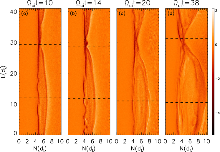
Figure 1: Snapshots of $J_{eM}$, the dawn-dusk electron current density, in one $L-N$ plane. (a–d) Taken at $t=10$, $14$, $20$, and $38$, respectively. These times highlight the onset of the instability, a time of maximum growth, a decrease in power, and the end of the simulation. The colors in each panel are identically normalized, with the color bar at the right showing the range. The dashed lines in each panel indicate the locations of cuts through the X line and island presented in Figure 2.

The instability driving the turbulence is electromagnetic in nature, as can be seen in Figure 2. Figures 2a–2h show $E_{M}$ and $\delta B_{L}$ in the $M-N$ plane that cuts through the X line, while Figures 2i–2p show the same quantities along a cut through the island. Here, $\delta B_{L}$ is the fluctuating component of $B_{L}$, that is, $\delta B_{L}=B_{L}-\langle B_{L}\rangle$, where $\langle B_{L}\rangle$ is $B_{L}$ averaged over the $M$ direction. This is the dominant magnetic field perturbation—convection of the large gradient of $B_{L}$ in the initial state due to the perturbed $v_{eN}$ leads to large fluctuations. Fluctuations of $B_{M}$ and $B_{N}$ are also present but at a reduced amplitude (Price et al., 2016).

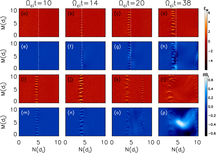
Figure 2: Snapshots of (a–d, i–l) $E_{M}$, the electric field in the direction of the reconnection-associated current, and (e–h, m–p) $\delta B_{L}$, the fluctuations in the reconnecting magnetic field, in the $M-N$ plane at the same times as in Figure 1. The cuts were taken at the positions shown by the dashed lines in Figure 1. Figures 2a–2h are taken at the $L$ location of the x-line, while Figures 2i–2p are taken through the middle of the island. The red color bar corresponds to $E_{M}$, while the blue color bar corresponds to $\delta B_{L}$. The dotted lines in Figures 2a–2h correspond to the $N$ location of the X line.

The turbulence first appears in both $E_{M}$ and $\delta B_{L}$ at $t=10$ along the magnetospheric separatrix in Figures 2i and 2m. Turbulence develops at the X line (Figures 2b and 2f) and along the magnetosheath separatrix (Figures 2j and 2n) by $t=14$, though the latter is clearer by $t=20$ (Figures 2k and 2o). It is interesting to note that even at relatively early times, the location of the turbulence begins to shift away from the X line, denoted by the white dotted lines in Figures 2a–2h, toward the magnetosphere. We also observe evidence of a possible kink mode late in the simulation in Figure 2p. This mode produces a global perturbation to the current sheet, but at longer wavelength than the fluctuations seen in the other panels.

The wavelength of the drift instability can be directly measured in several of the panels. In Figure 2b, for example, there are 11 wavelengths present in the $M$ direction (length $10.24d_{i}$). The choice of temperatures to use in the conversion from $d_{i}$ to $\rho_{e}$ is somewhat arbitrary due to the strong gradients in the system and the fact that the instability is a global mode across the magnetopause and along the local magnetic field (see Fig. 3). In this paper, since most of the plasma at the X line comes from there, we choose the asymptotic magnetosheath values. Other choices can change $\rho_{e}$ by up to a factor of 2. Thus, at $t=14$ in our mass ratio 100 simulation $1d_{i}\approx 27\rho_{e}$, which gives $k_{M}\rho_{e}\approx$ 0.25. As will be discussed later, this is consistent with the expectation for long wavelength LHDI.

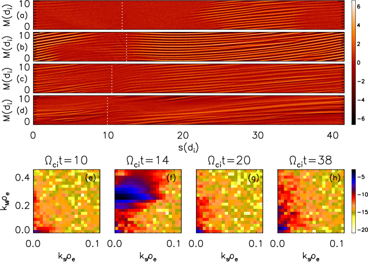
Figure 3: (a–d) $E_{M}(s,M)$ and (e–h) Fourier transforms at the same times as in Figure 1, where $s$ is the distance along the average (over $M$) magnetic field. The data are from a surface that lies to the left (magnetospheric side) of the magnetospheric separatrix. Figure 3a shows $E_{M}(s,M)$ at $t=10$; the $k_{s}-k_{M}$ power spectrum $\log(|\tilde{E}_{M}(k_{s},k_{M})|^{2})$ at the same time is shown in Figure 3e. Figures 3f, 3g, and 3h are similarly paired with Figures 3b, 3c, and 3d and show the simulation data at $t=14$, $20$, and $38$, respectively. The white dotted lines in Figures 3a–3d correspond to the location of the X line. Figures 3a–3d are normalized to the same value, as seen in their accompanying color bar. Figures 3e–3h also have a common normalization.

While LHDI is the most likely candidate to explain the turbulence seen in our simulations, the modified-two-stream instability (MTSI) can also exist in finite $\beta$ systems if the relative cross-field drifts of the electrons and ions are comparable to or exceed the local Alfvén speed (Wu et al., 1983). It has been suggested that this instability is important in laboratory reconnection experiments (Ji et al., 2004). This instability has a growth rate that peaks with a nonzero component of the wave vector along the local magnetic field $k_{\parallel}$ in contrast with the LHDI, which has a peak growth rate for $k_{\parallel}=0$ (Daughton, 2003). Thus, to distinguish between the possible drivers of the turbulence, we examine its Fourier spectrum perpendicular to and along the local magnetic field in $k_{\perp}-k_{\parallel}$ space, where $k_{\perp}$ is calculated from the data along the $M$ direction. Since the local direction of the magnetic field varies in space, the necessary data must be taken while following a magnetic field line. Furthermore, since the actual field lines have chaotic trajectories (Price et al., 2016), the analysis is carried out using the magnetic field components obtained by averaging over the $M$ direction. The averaged magnetic field on the magnetospheric side of the reconnection layer follows the separatrix between the upstream and reconnected plasma, while $M$ points in the perpendicular direction. Choosing $s$ to represent the distance measured along the field, we construct $E_{M}(s,M)$ while traveling along a field line just outside the separatrix. The range of $s$ is chosen in order to travel through the simulation domain in the $L$ direction exactly once. These data are not periodic in $s$ for a given value of $M$, but the data can be extended arbitrary distances along $s$ by stacking the data along $s$ if it is shifted a fixed distance in $M$.

The resultant $E_{M}(s,M)$ at four times can be seen in Figures 3a–3d. The primarily horizontal stripes correspond to the same instability shown in Figure 2. In Figure 3a, calculated at $t=10$, the instability is weak at the location of the X line (the white dotted line) but strong near the middle of the island (see Figure 1a). By $t=14$ in Figure 3b the instability is present at all values of $s$, including at the X line, although it remains strongest near the middle of the island. This pattern persists at later times, $t=20$ and $38$, Figures 3c and 3d, respectively, making it appear that the turbulence near the X line is not strong. However, note that as seen in Figures 2c and 3d, the turbulence at these times is displaced from the separatrix. Although not shown here, $E_{M}(s,M)$ at the X line is much stronger along a trajectory that is displaced toward the magnetosphere compared with that shown in Figure 3.

To determine the dominant wavelengths present in $E_{M}(s,M)$, we construct two-dimensional spatial Fourier transforms (denoted by the operator $\mathcal{F}$) of the $s-M$ domain, $\tilde{E}_{M}(k_{s},k_{M})=\mathcal{F}[E_{M}(s,M)]$. We plot $\log(|\tilde{E}_{M}(k_{s},k_{M})|^{2})$ for the longest wavelength modes in Figures 3e–3h. At $t=10$, Figure 3e, which is the linear stage of the instability, the spectrum is dominated by nearly perpendicular wave vectors (note the difference in vertical and horizontal axis scales). The peak power when the instability is strongest, $t=14$, occurs for $k_{M}\rho_{e}~{}\approx 0.25$, consistent with the calculation based on Figure 2. By this time the spectrum has acquired a significant parallel wavevector ($k_{s}$), although it continues to be dominated by perpendicular modes. After saturation (Figures 3g and 3h), however, those parallel modes diminish in strength. Since this simulation employs an ion-to-electron mass ratio of $100$, theory suggests that the longer wavelength LHDI mode has $k_{M}\rho_{e}\sim(m_{e}T_{e}/m_{i}T_{i})^{0.25}\approx 0.14$. As before, we employ the asymptotic magnetosheath temperatures since LHDI is a global mode. The expected value is consistent with our measured value of $k_{M}\rho_{e}\approx 0.25$.

The nonlocal structure of the MTSI has not been explored in the literature. Nevertheless, in local models the instability peaks at $k_{\parallel}/k_{\perp}\sim\sqrt{m_{e}/m_{i}}$ (Wu et al., 1983). For the simulation data shown in Fig. 3 in which $m_{i}/m_{e}=100$ the spectrum should exhibit a distinct peak centered on $k_{s}\sim 0.1k_{M}$ if it were driven by the MTSI. There is no evidence for a peak at finite $k_{\parallel}$ in the data of Fig. 3.

However, the data of Fig. 3 do reveal that $k_{s}$ is finite. We suggest that this is a consequence of the inhomogeneity of the out-of-plane current with distance along the separatrices. As discussed in Price et al. (2016), this instability dominantly drives flows in the $M-N$ plane. The resulting twisting of flux ropes by the vortical $M-N$ flows is similar to that inferred from MMS observations by Ergun et al. (2016). The strength of the vortices varies with distance along the field line ($s$ direction) because the amplitude of the out-of-plane current $J_{eM}$ depends on the distance from the x-line. As a consequence, the rate of twist of the flux tubes varies with distance from the X line, generating nonzero values of $B_{M}$ and $B_{N}$ and a finite $k_{s}$.

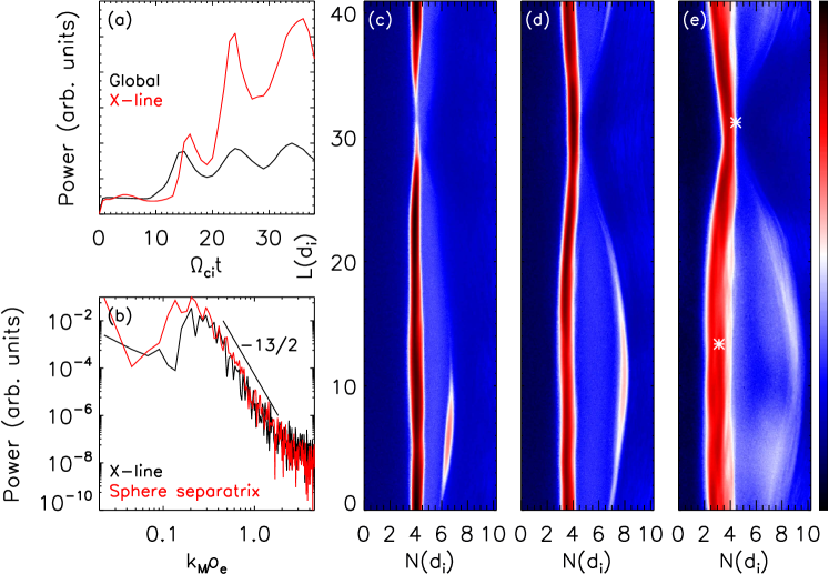
Figure 4: (a) Power in the instability as computed by equation (3), based on the fluctuating component of $\delta E_{M}=E_{M}-\langle E_{M}\rangle$ with $\langle\rangle$ denoting an average over the $M$ direction. The black line corresponds to the global power, while the red line corresponds to the power locally near the X line. (b) The one-dimensional power spectrum $\lvert\mathcal{F}\left[E_{M}(M)\right]\rvert^{2}$ at $t=34$, at the locations denoted by asterisks in Figure4e. The slope of the power law is around $-6.5$. (c–e) $\log\left(\sum_{M}(\delta E_{M})^{2}\right)$ at $t=14,24,$ and $34$, respectively. Figures 4c–4e have a common normalization.

The total power in the instability’s fluctuating electric field $\delta E_{M}=E_{M}-\langle E_{M}\rangle$,

$$P=\sum_{L,M,N}(\delta E_{M})^{2},$$ (3)

where $\langle\rangle$ denotes an average over the $M$ direction, is computed for the duration of the simulation and plotted in Figure 4a. The power is calculated both globally (the black curve) and for a small region around the X line ($N\in(2,5)$, $L\in(27,36)$, the red curve). The global power begins to increase at $t=10$, first peaks at $t=14$, and decreases to a local minimum at $t=20$, before reaching new peaks at $t=24$ and $34$. The same pattern is observed in the power at the X line, albeit offset slightly in time. This is consistent with Figures 1 and 2, with the instability first appearing along the magnetospheric separatrix before developing at the X line. The overall increase in the baseline (nonoscillatory) power seen at the X line is due to the spreading of the turbulence over a greater spatial domain and not to an increase in the turbulence’s amplitude; the amplitude saturates around $t=14$. The relative magnitudes of the two curves are not significant. Instead, what is important is their profile in time. The periodicity observed here corresponds to a slow oscillation, or “breathing,” of the current sheet in the $N$ direction and is also observed in calculations of the reconnection rate (not shown). This “breathing” is a consequence of the absence of a kinetic equilibrium in the initial state. Figure 4b shows the one-dimensional power spectrum $\lvert\mathcal{F}\left[E_{M}(M)\right]\rvert^{2}$ at $t=34$ at both the X line and the magnetosphere separatrix. The spectrum takes the form of a power law with a slope of around $-6.5$, which is the same at both the X line and the separatrix. A power law in the frequency spectrum of turbulence associated with the LHDI has been seen in the Polar spacecraft data at the magnetopause (Bale et al., 2002) although the spectral index was much harder, $-1$, in comparison to the spectrum here. Figures 4c–4e show $\log\left(\sum_{M}(\delta E_{M})^{2}\right)$ at the times of the three peaks, representing the strength of the fluctuations in $E_{M}$. As in Figure 2, the fluctuations first appear strongest along the magnetosphere separatrix (Figure 4c) but also appear weakly along the magnetosheath separatrix. At late time the fluctuations are also evident within the reconnection exhaust as turbulence around the X line and magnetic separatrices is carried into the exhaust. A filamentary exhaust has been documented in MMS observations (Phan et al., 2016).

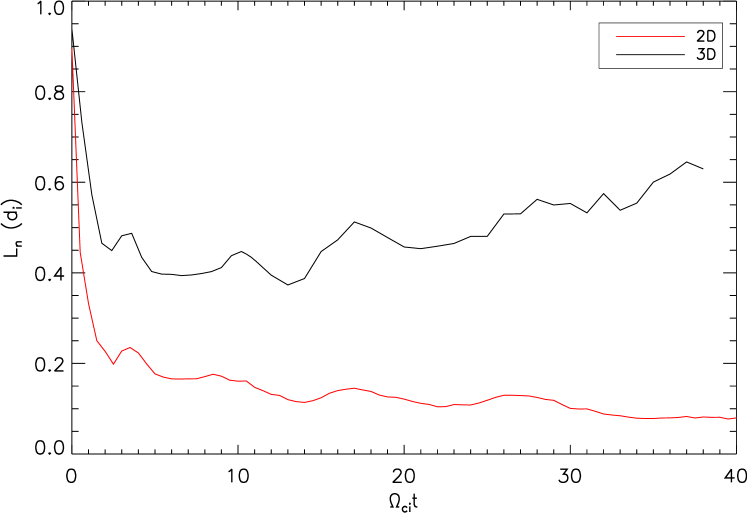
Figure 5: The density scale length $L_{n}$ as a function of time for the mass ratio 100 simulations.

As discussed earlier, the energy source for the instability is the relative electron-ion drift, which is dominantly produced by the ion pressure gradient. Because of the large drop in the density across the magnetopause for the initial conditions of the present simulation, the ion pressure drop is dominated by the change in density. We therefore explore the linkage between the time evolution of the density profile and the development of the turbulence to demonstrate the causal relation between the local gradient and the turbulence. Figure 5 shows the density scale length at the X line as a function of time for the 3-D and 2-D mass-ratio 100 simulations.

For the 3-D simulation, the initial density scale length $L_{n}$ ($\approx 1d_{i}=10d_{e}$) decreases as reconnection develops, reaching its minimum value ($L_{n}\approx 0.4d_{i}=4d_{e}$) at $t=13$, near when the instability is strongest. The density profile then relaxes somewhat and by the end of the simulation $L_{n}\approx 0.6d_{i}=6d_{e}$. Similar behavior is observed for a 3-D simulation with mass ratio 400 (not shown). This result should be contrasted with the results of the 2-D simulation with the same parameters, in which turbulence does not develop and in which the density gradient steepens in time and comes to a constant density scale length of around $L_{n}\approx 0.1d_{1}=1.0d_{e}$. Thus, the turbulence clearly limits the minimum density scale length and the corresponding width of the electron current layer. We note that because of their high cadence, the MMS spacecraft instruments reveal the local density in a cut across the magnetopause rather than the average scale length shown in Fig. 5. However, the rate of large-scale reconnection is controlled by the $M$-averaged properties of the system, including the $M$-averaged density. This point will be emphasized below in the discussion of averaged and local Ohm’s law for this event.

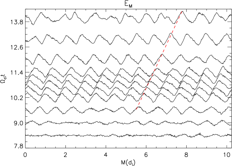
Figure 6: Cuts of $E_{M}$ along the $M$ direction through the center of the turbulence at the magnetospheric separatrix. The vertical position of each cut is shifted based on the time at which it was taken. The red dashed line traces the displacement of one wave peak.

Next we calculate the phase speed and frequency of the instability. Figure 6 shows cuts of $E_{M}$ along the $M$ direction through the center of the turbulence at the magnetospheric separatrix near the middle of the island. The vertical position of each cut corresponds to the time at which it was taken. The turbulence begins to appear over the background variations at $t\approx 9$ and by $t=10$ has clearly developed linear oscillations. The topmost trace, at $t\approx 14$, is taken when the instability is strongest. The irregular variations show that it has already reached a nonlinear stage, and by this time the wave potential is larger than the electron thermal energy. By tracing the displacement of one wave peak (the red dashed line), we determine the phase velocity of this wave to be $v_{p}\approx\frac{1}{2}v_{A}$ in the direction of the electron diamagnetic drift. This value is not specific to the wave peak chosen; similar results are obtained by translating the red dashed line in the $M$ direction to adjacent peaks. Thus we can compute the instability frequency in the frame of the simulation $\omega=v_{p}k_{M}\approx 0.25\Omega_{\text{lh}}$.

This differs significantly from $\Omega_{\text{lh}}$, which is the textbook frequency of the LHDI. There are two reasons for this. The first is that, as discussed in Daughton (2003), electromagnetic LHDI modes are not fixed at $\Omega_{\text{lh}}$ but can instead have frequencies anywhere in the range $\omega_{\text{ci}}\leq\omega\leq\Omega_{\text{lh}}$. Second, the standard derivation of the frequency of LHDI is performed in a frame with $E_{N}=0$, which is not the case at the magnetopause and is not true for our simulation. In the $E_{N}=0$ frame, the ions have the strongest drift, of the order of the ion diamagnetic drift velocity (which exceeds the electron diamagnetic velocity because the ions are hotter than the electrons). In our system, the ions are close to stationary, so the observed frequency is naturally lower than the lower hybrid frequency found in the typical analysis. Further, the mode propagates in the electron direction, which is consistent with MMS observations of fluctuations at the magnetopause (Graham et al., 2017). In our simulation it is not possible to completely transform away $E_{N}$ since this would require $cE_{N}/B_{L}$ to be a constant. It is possible, however, to transform our simulation results into a frame in which the value of $E_{N}$ is greatly reduced. At the magnetospheric separatrix during the time of linear evolution, $c({E}\bm{\times}{B})_{M}/B^{2}\approx cE_{N}/B_{L}$ has a peak value of around $-1.7v_{A}$. In a frame with this velocity, the phase speed of the wave is $\approx 1.2v_{A}$, giving a frequency of $\omega=0.6\Omega_{\text{lh}}$, closer to the expected value.

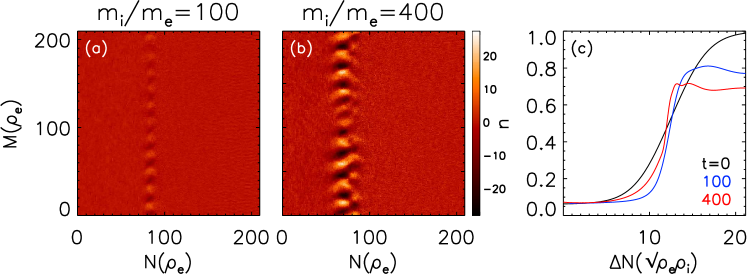
Figure 7: Comparison between the $m_{i}/m_{e}=100$ and $400$ simulations. (a–b) Snapshots of $E_{M}$ in the $M-N$ plane through the X line at times of maximum power for $m_{i}/m_{e}=100$ (Figure 7a) and $400$ (Figure 7b). The numerical values of $E_{M}$ have been converted to units of mV/m. (c) Density profiles at the X line at $t=0$ and times of minimum density scale length. The density profiles have been shifted in $N$ to facilitate comparison.

In Price et al. (2016), we suggested that the qualitative features of a real mass ratio simulation would not differ significantly from one with $m_{i}/m_{e}=100$. Although we find that conclusion still holds, there are important quantitative differences between the simulation discussed in detail above (mass ratio of 100) and one with mass ratio 400. Figures 7a and 7b show $E_{M}$ in the $M-N$ plane through the X line for mass ratio 100 (Figure 7a) and 400 (Figure 7b) at times of maximum power (as determined using equation (3)). While the simulation domains differ in size when measured in $d_{i}$, they are equivalent when measured in $\rho_{e}$. The instability is stronger in the mass ratio 400 case and the turbulence has a greater spread in the $N$ direction. As before, the wavelength of the instability can be visually determined. In Figure 7b there are 10 wavelengths in the $M$ direction (length $\approx 282\rho_{e}$), giving $k_{M}\rho_{e}\approx 0.22$. In agreement with theoretical expectations there are fewer wavelengths (10 versus 11) and smaller $k_{M}\rho_{e}$ for the more realistic mass ratio. Furthermore, by constructing $E_{M}(s,M)$ and $\log(|\tilde{E}_{M}(k_{s},k_{M})|^{2})$ (not shown), we find that the peak of the instability occurs at $k_{M}\rho_{e}\approx 0.22$. For an ion-to-electron mass ratio of 400, the longer wavelength LHDI mode is expected to satisfy $k_{M}\rho_{e}\sim(m_{e}T_{e}/m_{i}T_{i})^{0.25}\approx 0.09$. Note though that as discussed below, the ambient density gradient also varies between the two simulations so the scaling $k_{M}\rho_{e}\sim(m_{e}T_{e}/m_{i}T_{i})^{0.25}$ is only approximate.

The scale lengths of the density and current layers at the magnetopause are topics of scientific interest since they are linked to the processes that limit the electron current. As noted previously, our 2-D simulations show that density scale length is of order $1d_{e}$, which is the expected value during reconnection without turbulence. The current layers in the 3-D simulations are limited by the development of turbulence and never reach electron scales. Because our simulations are carried out with artificial mass ratios, care must be taken in interpreting the data. In Figure 7c we display density profiles at the X line for our mass ratio $100$ and $400$ simulations. The initial density profile is the same for both simulations. The profiles displayed for each mass ratio are chosen to correspond to the time when the density gradient is greatest. The horizontal length scale is measured in hybrid units, $\sqrt{\rho_{e}\rho_{i}}$. Thus, the minimum scale length of the density profile (and the current profile) during reconnection at the magnetopause appears to scale as the hybrid of the electron and ion Larmor radii rather than either the electron or ion scale. However, because of the weak dependence of this scaling on the mass ratio and the limited mass ratios explored in the simulations, there is some uncertainty in this conclusion. Nevertheless, the current and density scale lengths at the magnetopause are significantly greater than the expected $d_{e}$ or $\rho_{e}$ scale. Further, the widths are comparable to measurement of the widths of current layers during symmetric reconnection in the magnetosheath (Phan et al., 2007) and in a laboratory reconnection experiment (Ren et al., 2008). Consistent with the simulation results the analysis of MMS observations at the magnetopause also suggested that such turbulence was responsible for electron transport across the X line from the magnetosheath into the magnetosphere (Graham et al., 2017).

IV Discussion

As discussed previously, we have demonstrated that the turbulence that develops during 3-D simulations of the MMS 16 October 2015, reconnection event is strong enough to control the characteristic layer widths at the magnetopause. We now address whether the turbulence is strong enough to impact the effective Ohm’s law controlling large-scale reconnection. Our previous analysis of simulations of this event (Price et al., 2016) considered the effects of the turbulence on reconnection by evaluating the contributions of various terms to an averaged Ohm’s law measured within the electron diffusion region. The $M$ component of Ohm’s law (the electron equation of motion) is as follows:

$$E_{M}=-\frac{1}{c}(\mathbf{v_{e}}\bm{\times}\mathbf{B})_{M}-\frac{1}{ne}(\bm{\nabla\cdot}\mathbb{P}_{e})_{M}-\frac{1}{e}m_{e}\mathbf{v_{e}}\bm{\cdot\nabla}v_{eM}.$$ (4)

Here $m,n,\mathbf{v_{e}}$ and $\mathbb{P}_{e}$ are the electron mass, density, velocity, and pressure tensor. Because the temporal evolution of the turbulence is over a short time scale compared with the time associated with large-scale reconnection, large-scale reconnection is controlled by the Ohm’s law that is averaged over the turbulence. This assumption is normally satisfied since the turbulence is at the $\rho_{e}$ scale with a frequency $\Omega_{\text{lh}}$, while large-scale reconnection takes place on time scales longer than the Alfvén transit time across the computational domain. For 3-D simulations the average is evaluated by averaging Ohm’s law over the $M$ direction. As discussed earlier for the fluctuating $E_{M}$, we carry out this average by separating each quantity in Ohm’s law into fluctuating and averaged quantities, $f=\langle f\rangle+\delta f$ and then averaging Eq. 4 over $M$. In addition to contributions independent of the fluctuations (the usual laminar contributions to Ohm’s law) are terms quadratic in the fluctuations that correspond to the anomalous drag $-\langle\delta n_{e}\delta E_{M}\rangle$ and anomalous viscosity $\langle m{\bf\nabla}\cdot(\delta{\bf J}_{e}\delta v_{M})/e+\delta J_{eN}\delta B_{L}/c+\delta J_{eL}\delta B_{N}/c\rangle$. The conclusion from earlier simulations of this event (Price et al., 2016; Le et al., 2017) was that the anomalous terms were important during the early phase of reconnection. However, Le et al. (2017) found that the turbulence weakened at late time so that the anomalous terms were no longer important. In Fig. 8a we show late time ($\Omega_{ci}t=38$) cuts of various parameters from the simulations ($B_{L}$, $E_{N}$, $v_{eM}$, $v_{eN}$, and $n_{e}$) versus $N$ in a cut through the X line. The vertical dashed lines correspond to the locations of the X line and the electron stagnation point $v_{eN}=0$, which are displaced (Cassak and Shay, 2007). In Fig. 8b are the various contributions from the averaged Ohm’s law. The electron diffusion region is the entire domain where the dominant laminar terms $e\langle n_{e}\rangle\langle E_{M}\rangle$ and $\langle J_{eN}\rangle\langle B_{L}\rangle/c$ do not balance. This region extends well past the magnetosphere side of the stagnation point. The laminar pressure tensor term which dominates the 2-D simulations continues to be significant in the 3-D system. The anomalous viscosity term is large across the entire region between the X line and stagnation point, while the drag contribution is large on the magnetosphere side of the stagnation point. Finally, in Fig. 8c we show that the total of all of the terms in the averaged Ohm’s law balance the average $E_{M}$ at this time. Thus, we reach a different conclusion than Le et al. (2017). The turbulence remains strong enough to significantly impact Ohm’s law even at late time. The reason for the discrepancy is unknown.

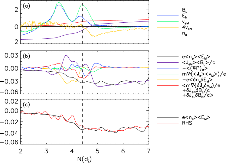
Figure 8: Cuts along the N direction through the X line at $\Omega_{ci}t=38$. (a) $B_{L}$, $E_{N}$, $v_{eM}$, $v_{eN}$, and $n_{e}$ where the vertical dashed lines mark the X line and stagnation point $v_{eN}=0$. (b) The various contributions from the $M$ component of the averaged Ohm’s law. (c) Sum of the various contributions to the average of the right-hand side of Ohm’s law in Eq. (4) compared to $e\langle n_{e}\rangle\langle E_{M}\rangle$.

Before making further comparisons between the simulations and the MMS data, we must establish the correspondence between the units used in the simulation and those used in spacecraft measurements. For the asymptotic parameters of the 16 October 16 2015 event ($B_{L,\text{sh}}\sim 23\text{ nT}$, $B_{L,\text{ms}}\sim 39\text{ nT}$, $n_{\text{sh}}\sim 11.3/\text{cm}^{3}$, $n_{\text{ms}}\sim 0.7/\text{cm}^{3}$) with “sh” and “ms” subscripts denoting the magnetosheath and magnetosphere respectively, $d_{e,\text{sh}}\sim 1.6\text{ km}$, $d_{i,\text{sh}}\sim 68\text{ km}$, $\omega_{ce,\text{sh}}\sim 4.05\text{ kHz}$, $\Omega_{\text{lh},\text{sh}}\sim 95\text{ Hz}$, $\omega_{ci,\text{sh}}\sim 2.2\text{ Hz}$, $v_{A,\text{sh}}\sim 150\text{ km/s}$ and $E_{0,\text{sh}}\sim 3.4\text{ mV/m}$. In our simulations we find a reconnection electric field of $\sim 0.2\text{ mV/m}$ for either mass ratio, a value that would be very difficult to detect observationally. In fact, MMS observations reveal spikes in $E_{M}$ with much larger values, peaking around $\pm 10\text{ mV/m}$. In addition, large amplitude, short-timescale fluctuations of the parallel electric field $E_{\parallel}$, up to $100\text{ mV/m}$, have been reported (Ergun et al., 2016, 2017). These intense parallel electric fields are not observed in our simulations.

The question, then, is whether the MMS electric field measurements correspond to an effective average over the turbulence in the simulation or a slice at a particular value of $M$. To answer this question, note that the particle instruments on MMS directly measure the full distribution function of electrons in $30\text{ ms}$ and of ions in $150\text{ ms}$. The frequency $\omega$ of the fluctuations in the simulation is around $\frac{1}{4}\Omega_{\text{lh},\text{sh}}=24\text{ Hz}$ so the period of the waves is around $260\text{ ms}$. Thus, the electron data are collected over a very short period compared to the wave period. The MMS instruments are therefore measuring the local electron Ohm’s law and not the average Ohm’s law that controls the global reconnection rate.

To understand the challenge associated with deducing the global reconnection rate directly from the MMS data, we translate the reconnection rate determined from our simulation into real units. The electric field in the simulation in SI units is normalized to $E_{0}=B_{L,\text{sh}}c_{A,\text{sh}}$. For $B_{L,\text{sh}}=23\text{ nT}$ and $n_{\text{sh}}=11.3/\text{cm}^{3}$, $c_{A,\text{sh}}=150\text{ km/s}$ and $E_{0}=3.4\text{ mV/m}$. Thus, based on Figure 8c, we obtain the reconnection electric field $E_{\text{rec}}=0.17\text{ mV/m}$. Extracting such a very small electric field directly is problematic first because it is small and second because the turbulent fluctuations in the electric field are typically of order of $10\text{ mV/m}$ or higher (Burch et al., 2016; Ergun et al., 2016, 2017; Graham et al., 2017). Similarly, we can translate the drag term in Fig. 8b into the units of an effective electric field, which yields $0.15\text{ mV/m}$. The evaluation of the drag from direct measurements is a challenge because it is necessary to carry out a time average of the correlation of the product of the fluctuations. This was carried out earlier using THEMIS magnetopause data (Mozer et al., 2011) and more recently using MMS data (Graham et al., 2017). The effective drag electric field was around $0.5\text{ mV/m}$ in the more recent analysis from MMS. However, the average was evaluated by simply averaging over the four spacecraft and using a low-pass filter. Thus, the result was noisy and therefore probably not very reliable. Further, the authors concluded that the drag terms were small in comparison with the local values of the electric field and therefore unimportant. As discussed previously, however, the drag terms only apply to the analysis of the large-scale reconnection electric field, which based on the simulation is of order $0.17\text{ mV/m}$. Thus, on this basis the measured drag terms are large enough to balance the large-scale reconnection electric field.

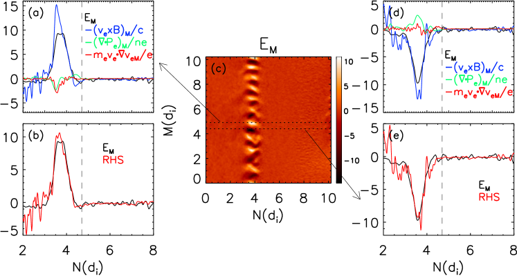
Figure 9: Evaluation of Ohm’s law on cuts through the region of instability. For direct comparison to data, values are converted from our normalized units to mV/m. (a) The terms in Ohm’s law from equation (4) for a cut through $M=4.9$. (b) The sum of the left and right sides of equation (4) for $M=4.9$. (c) $E_{M}$ in the $M-N$ plane at $t=38$. The horizontal dotted lines denote locations of two cuts, at $M=4.4$ and $4.9$. (d) The terms in Ohm’s law from equation (4) for a cut through $M=4.4$. (e) The sum of the left and right sides of equation (4) for $M=4.4$. The vertical dashed lines in Figures 9a–9b and 9d–9e indicate the position of the X line.

In order to determine the structure of the local Ohm’s law and therefore what MMS would measure within the diffusion region, we examine the various terms in the $M$ component of Ohm’s law in equation (4) in a cut through the X line. We emphasize that this does not represent the actual time dependence of the measurements from MMS but is meant to emphasize the significant differences between the averaged Ohm’s law and that from a local measurement. In Figure  9 we present data from two sample cuts through the electron diffusion region along the $N$ direction. Figure 9c shows $E_{M}$ near the X line in the $M-N$ plane at $t=38$. Figure 9a displays the separate terms in Ohm’s law (equation ((4))) at $M=4.9$ along a cut in the $N$ direction (the upper dashed line in Figure 9c). Figure 9b shows $E_{M}$ and the sum of the terms from the right-hand side of equation (4). The two curves are in close agreement, which confirms that the simulation data are consistent with momentum conservation based on the electron equation of motion. Note also that the vertical scale is expressed in mV/m so the curves reflect the size of the terms that should be visible in the MMS data. Figures 9d and 9e show the same information for a cut through $M=4.4$. The value of $E_{M}$ peaks around $\pm 10\text{ mV/m}$, very close to the values reported in the MMS data (Burch et al., 2016). The peak value of $E_{M}$ changes sign between the two cuts, which are separated by a distance roughly comparable to the distance between the MMS spacecraft. Interestingly, a similar difference in polarity is seen in the MMS data (see Figure 5 of Burch et al. (2016)). It should be emphasized that the large value of $E_{M}$ shown in these cuts is a result of the turbulence and does not reflect the rate of magnetic reconnection. The reconnection electric field, while present, is 2 orders of magnitude smaller and can only be extracted by the type of averaging discussed above.

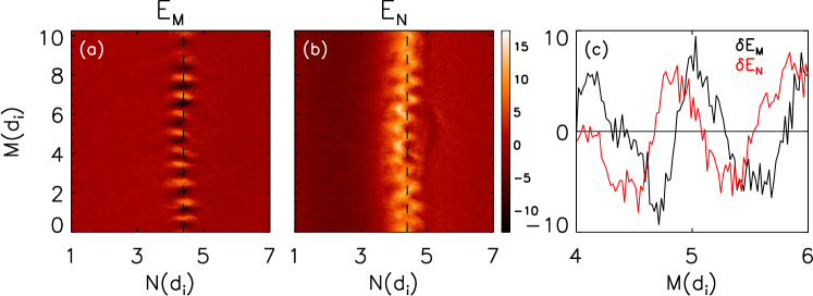
Figure 10: (a) $E_{M}$ and (b) $E_{N}$ in the $M-N$ plane at the X line at $t=20$. For direct comparison to data, values are converted from our normalized units to mV/m. (c) $\delta E_{M}$ and $\delta E_{N}$ through the vertical dashed line in Figures 10a and 10b. Figures 10a and 10b are normalized to the same value.

As a further demonstration that $E_{M}$ is primarily associated with the turbulence, Figure 10 shows $E_{M}$ and $E_{N}$ (Figures 10a and 10b) in the $M-N$ plane near the X line at $t=20$. In Figure 10c we plot cuts of $\delta E_{M}$ and $\delta E_{N}$ at the locations denoted by the vertical dashed lines in Figures 10a and 10b. As the current layer breaks up, it naturally produces large values of $E_{M}$ as the large electron currents in the $M$ direction are diverted into the $N$ direction. These $N$-directed flows are driven by $E_{M}$. The fact that $\delta E_{M}$ and $\delta E_{N}$ are similar in magnitude and roughly $90^{\circ}$ out of phase indicates that the fluctuations are linked and not due to a steady-state reconnection process. Of course, the turbulence itself might undergo reconnection on faster time scales and produce electric fields larger than the nominal value of 0.1 mV/m. Such a possibility requires further analysis and comparison with observations.

Multiple MMS observations of magnetopause electron diffusion regions have found features similar to those in Figure 9 (Ergun et al., 2017). Since the observed turbulence did not satisfy the properties of homogeneous LHDI it was suggested that some other mechanism was responsible. However, the findings presented here suggest that the governing instability has all of the characteristics of a longer wavelength version of LHDI. The instability has a dominant wavelength satisfying $k\rho_{e}\approx(m_{e}T_{e}/m_{i}T_{i})^{0.25}$, is observed in both electric and magnetic field components and has a wave vector that is dominantly, but not strictly, perpendicular to the local magnetic field. The frequency of the instability falls in the range of frequencies unstable to LHDI, $\omega_{\text{ci}}\leq\omega\leq\Omega_{\text{lh}}$ and the growth of the instability is closely correlated with the steepening and relaxing of a density gradient (and therefore the ion pressure gradient, which is the basic driver of drift instabilities at the magnetopause). Similar instabilities have been seen in other three-dimensional reconnection simulations (albeit with different initial conditions) and were also attributed to LHDI (Daughton, 2003; Pritchett et al., 2012; Le et al., 2017).