Masses of Kepler-46b,c from Transit Timing Variations

Abstract

We use 16 quarters of the Kepler mission data to analyze the transit timing variations (TTVs) of the extrasolar planet Kepler-46b (KOI-872). Our dynamical fits confirm that the TTVs of this planet (period $P=33.648^{+0.004}_{-0.005}$ days) are produced by a non-transiting planet Kepler-46c ($P=57.325^{+0.116}_{-0.098}$ days). The Bayesian inference tool MultiNest is used to infer the dynamical parameters of Kepler-46b and Kepler-46c. We find that the two planets have nearly coplanar and circular orbits, with eccentricities $\simeq 0.03$ somewhat higher than previously estimated. The masses of the two planets are found to be $M_{b}=0.885^{+0.374}_{-0.343}$ and $M_{c}=0.362^{+0.016}_{-0.016}$ Jupiter masses, with $M_{b}$ being determined here from TTVs for the first time. Due to the precession of its orbital plane, Kepler-46c should start transiting its host star in a few decades from now.

1 Introduction

More than 3300 exoplanets have been discovered with the Kepler and K2 missions, and almost 16% of these are in multi-transiting planetary systems with at least two confirmed planets (exoplanetarchive.ipac.caltech.edu) The detection of these exoplanets was possible because they have nearly edge-on orbits and pass in front of the star, thus producing a dip in the photometric light curve. The analysis of the transit light curve allows scientists to determine the planetary to stellar radius ratio (${R_{P}}/{R_{\star}}$), the inclination of the planetary orbit ($i_{P}$), the transit duration ($t_{D}$), and the time of mid-transit ($t_{C}$) (e.g., Seager & Mallén-Ornelas 2003, Carter et al. 2008).

In multi-planetary systems, the mutual gravitational perturbation between planets can be detectable under certain conditions. For example, the mid-transit time $t_{C}$ of consecutive transits of the same planet may not occur exactly on constant ephemeris. Instead, due to the gravitational perturbations from planetary companions, $t_{C}$ values can display non linear trends called Transit Timing Variations (TTVs). In some cases, it is also possible to measure variations of $t_{D}$, known as the Transit Duration Variations (TDVs), which can also be attributed to the gravitational perturbations.

The dynamical analysis of TTVs can yield a comprehensive characterization of orbits and also the planetary masses, or at least provide certain limits (Miralda-Escudé 2002, Agol et al. 2005, Holman & Murray 2005). The TTVs have been primarily used to confirm and characterize the systems of multi-transiting planets (Holman et al. 2010, Lissauer et al. 2011, Steffen et al. 2012, Xie 2014), but they can also be used to detect and characterize non-transiting planets (Ballard et al. 2011, Nesvorný et al. 2012, 2013, 2014, Dawson et al. 2014, Mancini et al. 2016). In fact, if the radial velocity measurements are not available, the observation and analysis of TTVs provide the only way currently available to determine masses. When the mass determination is combined with the planetary radius estimate from the transit light curve, this results in a planetary density estimate, and hence allows scientists to develop internal structure models (e.g. Guillot & Gautier 2015).

In this work, we focus on the Kepler-46 system (KOI-872). The first analysis of the light curve of Kepler-46 showed the presence of a candidate planet, currently known as Kepler-46b, with a 33.6 day period and radius consistent with a Saturn-class planet (Borucki et al. 2011). Nesvorný et al. (2012) measured and analyzed the TTVs and TDVs of 15 transits from Kepler quarters 1-6. They found that the TTVs can be best explained if Kepler-46b is a member of a two-planet system with the planetary companion, Kepler-46c, having a non-transiting orbit on outside of Kepler-46b. The TTVs analysis provided two possible solutions for the orbital parameters of the two planets, but one of these solutions was discarded by Nesvorný et al. because it produced significant TDVs, which were not observed. The preferred solution indicates a nearly coplanar ($I_{\mathrm{mut}}\simeq 1^{\circ}$) and nearly circular ($e\simeq 0.01$) orbits, and $M_{c}=0.376^{+0.021}_{-0.019}$ $M_{\mathrm{J}}$. The mass of Kepler-46b was not constrained from TTVs/TDVs, but an upper limit of $M_{b}<6$ $M_{\mathrm{J}}$ was determined from the stability analysis.

Here, we reanalyzed the Kepler-46 system using 35 transits from Kepler quarters. The transit analysis and dynamical fits were executed using MultiNest (Feroz et al. 2009, 2013), which is an efficient tool based on the Bayesian inference method. We were able to better determine the orbital parameters and masses of the two planets. The mass of Kepler-46b was determined here from TTVs for the first time. The paper is organized as follows: in Section 2, we describe the light curve analysis to obtain the mid-transit times and transit parameters of Kepler-46b. In Section 3, we discuss the dynamical analysis. The results are reported in Section 4. The last section is devoted to the conclusions.

2 Light curve analysis and transit times

Table 1: The mid-transit times $t_{C}$ obtained for Kepler-46b from the analysis of Kepler Quarters 1-16(Model $\mathcal{M}_{I}$).

Cycle	$t_{C}$ (BJD)
1	$55019.6993\pm 0.0012$
2	$55053.2959\pm 0.0010$
3	$55086.8640\pm 0.0011$
4	$55120.4409\pm 0.0018$
6	$55187.6880\pm 0.0015$
7	$55221.3360\pm 0.0016$
8	$55254.9066\pm 0.0011$
9	$55288.4664\pm 0.0012$
11	$55355.6667\pm 0.0010$
12	$55389.3438\pm 0.0011$
13	$55422.9309\pm 0.0017$
14	$55456.4875\pm 0.0011$
15	$55490.0601\pm 0.0009$
18	$55590.9283\pm 0.0008$
19	$55624.5138\pm 0.0008$
20	$55658.0838\pm 0.0011$
21	$55691.6593\pm 0.0008$
22	$55725.3035\pm 0.0009$
23	$55758.9147\pm 0.0009$
24	$55792.5562\pm 0.0010$
25	$55826.1262\pm 0.0011$
26	$55859.6845\pm 0.0017$
27	$55893.2891\pm 0.0011$
29	$55960.5704\pm 0.0010$
31	$56027.7090\pm 0.0010$
32	$56061.2821\pm 0.0010$
33	$56094.8799\pm 0.0010$
35	$56162.1511\pm 0.0011$
36	$56195.7346\pm 0.0014$
37	$56229.3033\pm 0.0012$
38	$56262.8845\pm 0.0013$
39	$56296.5319\pm 0.0012$
40	$56330.1453\pm 0.0010$
41	$56363.7757\pm 0.0010$
42	$56397.3426\pm 0.0010$

Before a dynamical analysis can be conducted, the transit times and durations of each event need to be inferred. This, in turn, requires us to first detrend the Kepler photometry and then fit the transits with an appropriate model. For this task, we use a similar approach to that described in Teachey et al. (2017), which is essentially a modified version of the approach described in Kipping et al. (2013).

The broad overview is that we remove long-term trends from the Kepler simple aperture photometry with the CoFiAM algorithm described in Kipping et al. (2013). Essentially, CoFiAM is a cosine filter designed to not disturb the transit of interest but remove present longer-period trends. A pre-requisite for using CoFiAM is that the time and duration of each transit are already approximately known. Since this system is known to exhibit strong variations in both, this poses a catch-22 problem for us.

Following Teachey et al. (2017), we remedy the problem by conducting an initial detrending using approximate estimates for the times and a fixed duration taken from Nesvorný et al. (2014). This data are then fitted (as we will describe later) to provide revised estimates for the times and durations. These revised times and durations are then used as inputs for a second attempt at detrending the original Kepler data using CoFiAM again. This iteration process allows for self-consistent inference of the basic transit parameters.

Initially, we take into account the 40 transit events available for Kepler-46b (e.g. Holczer et al. 2016). However, one of such transit (corresponding to cycle 5) is found to have inadequately detrended data, which is identified by visual inspection of the light curve. Four other events (corresponding to cycles 0, 10, 16, and 28) are found to have insufficient temporal coverage. There are several reasons that this might happen. At first, safe modes and data downlinks cause genuine gaps in the time series. At the next level, any Kepler time stamp with an error flag not set to 0 is removed by CoFiAM. Then, CoFiAM puts a smoothed moving median through the data and looks for 3$\sigma$ outliers caused by sharp flux changes or some other weird behavior. Stitching problems among the quarters can also cause apparent sharp flux changes, and if we do not have enough usable data around the transit, then the event will also have data chopped this way. At last, the detrending of an event can fail giving a poor detrending, so we perform a second round of outlier cleaning that which may eventually lead to most of the data for that event being removed. In the end, we keep only 35 transits for which visual inspection of the light curve indicates that we would be able to get reliable time estimates (Table 1).

The actual fitting process, which is ultimately repeated twice, is conducted using MultiNest coupled to a Mandel & Agol (2002) light curve model. We assume freely fitted quadratic limb-darkening coefficients, using the prescription of Kipping (2013), and allow each transit to have a unique mid-transit time but a common set of basic shape parameters (i.e. a common duration). While 20 of the transits were short cadence, 15 were long cadence requiring re-sampling using the technique of Kipping (2010), for which we used $N_{\mathrm{resam}}=30$.

Since each transit requires a unique free parameter, this leads to a very large number of free parameters in the final fit (35 just for the times alone). For computational expedience, we split the light curve into 4 segments of 10 transits each, with 5 for the last segment. Each segment is independent of the others, but assumes internally consistent shape parameters. Rather than freely fitting each event, this allows for the transit template to be well constrained such that the mid-transit time precision is improved. We refer to the above model of segments of transits as model $\mathcal{M}_{S}$.

As we did in Nesvorný et al. (2014), we also try fitting each transit completely independently, but fixing the limb-darkening coefficients to the same as those used in Nesvorný et al. (2014). This allows for TDVs to be inferred as well as TTVs, but generally increases the credible interval of the TTV posteriors due to the much weaker information about the transit shape available. In what follows, we refer to this model as $\mathcal{M}_{I}$.

3 Dynamical analysis of transit times

Following Nesvorný et al. (2012), we proceed by searching for a dynamical model that can explain the measured transit times. At variance with Nesvorný et al., we do not fit the TTVs but we directly fit the mid-transit times, which is expected to be a more accurate procedure. The results presented in the following are based on the mid-transit times from model $\mathcal{M}_{I}$ (Table 1). We have performed similar computations using model $\mathcal{M}_{S}$ and verified that the results are indistinguishable within their 1-$\sigma$ uncertainties.

Table 2: Prior distributions of 12 model parameters that we used to obtain the dynamical fit. $\mathrm{U}[x,y]$ means a uniform distribution between $x$ and $y$. The subindex _P refers to any of the two planets.

Parameter	Prior values
$M_{P}/M_{\star}$	$\mathrm{U}[0,\,0.005]$
$P_{b}$ (days)	$\mathrm{U}[33.5,\,33.7]$
$P_{c}$ (days)	$\mathrm{U}[40,\,84]$
$e_{P}$	$\mathrm{U}[0,\,0.4]$
$b_{c}$	$\mathrm{U}[1,\,20]$
${\varpi}_{P}$ (∘)	$\mathrm{U}[0,\,360]$
$\lambda_{c}$ (∘)	$\mathrm{U}[0,\,360]$
$\Omega_{c}-\Omega_{b}$ (∘)	$\mathrm{U}[0,\,360]$
$\delta t$ (d)	$\mathrm{U}[-0.1,\,0.1]$

To perform the dynamical fit, we assume a model of two planet and we use a modified version of the efficient symplectic integrator SWIFT (Levison & Duncan 1994), adapted to record the mid-transit times of any transiting planet (Nesvorný et al. 2013, Deck et al. 2014). MultiNest is then used to perform the model selection and to estimate the best-fit values of the dynamical parameters with their errors.

MultiNest applies the Bayes rule (Appendix A) to determine the values of the 12 parameters of the model that are necessary to reproduce the observed mid-transit times. The method provides the posterior distributions of these 12 parameters, namely, the planet-over-star mass ratios (${M_{b}}/{M_{\star}}$, ${M_{c}}/{M_{\star}}$), the orbital periods ($P_{b}$, $P_{c}$), the eccentricities ($e_{b}$, $e_{c}$), the longitudes of periastron ($\varpi_{b}$, $\varpi_{c}$), the mean longitude and impact parameter of the non-transiting planet ($\lambda_{c}$, $b_{c}$), the difference of the nodal longitudes of the two planets ($\Omega_{c}-\Omega_{b}$), and the difference between the mid-transit time reference epoch ($\tau=55053.2826$ BJD) and the mid-transit time of the nearest transit ($\delta t$). This latter parameter gives us the information about the mean longitude of the transiting body at the reference epoch ($\lambda_{b}=\lambda_{b,0}-2\pi\,\delta t/P_{b}$, where $\lambda_{b,0}$ is the mean longitude at mid-transit time). The initial value of the impact parameter of Kepler-46b ($b_{b}$) is fixed at the value determined from the transit fit. We use the transit reference system from Nesvorný et al. (2012), where the reference plane is the plane defined by $b=0$, the origin of longitudes is at the line of sight, and the nodal longitude of Kepler-46b ($\Omega_{b}$) is set to $270^{\circ}$. The stellar parameters are also adopted from Nesvorný et al. (2012).

The priors distributions of the 12 model parameters are given in Table 2. The distributions were chosen as uninformative with uniform priors. The interval limits of these priors are based on results from Nesvorný et al. (2012) that guarantee that the system is constituted of a transiting and a non-transiting planet and is dynamically stable. The orbital period of the transiting body is well known from the transit fit, so we only consider a very small range of priors around the known value. For the period of the non-transiting planet, we consider an interval of priors that includes the two solutions found by Nesvorný et al. (2012). The upper limit in eccentricities is set to only 0.4, since higher values cause the code to become too slow and do not provide additional solutions. The upper limit of the impact parameter of the non-transiting planet corresponds to an inclination $i_{P}\sim 70^{\circ}$.

The calculation of the integrals involved in Eq. (A2) requires the use of a numerical method. MultiNest uses a multi-modal nested sampling technique to efficiently compute the evidence integral, and also provides the posterior distributions of the parameters. In our case, the likelihood function (see Appendix A) is defined as

$$L(d|\theta,M)=\prod_{j=1}^{N}\frac{1}{\sqrt{2\pi\sigma_{j}^{2}}}\exp\left(-\sum_{i=1}^{N}\frac{\left(t_{C,i}^{\mathrm{obs}}-t_{C,i}^{\mathrm{cal}}\right)^{2}}{2\sigma_{i}^{2}}\right),$$ (1)

where $N=35$ is the number of transits; $t_{C,i}^{\mathrm{obs}}$ and $t_{C,i}^{\mathrm{cal}}$ are the observed (Table 1) and calculated mid-transit times, respectively; and $\sigma_{i}$ is the uncertainty of $t_{C,i}^{\mathrm{obs}}$. According to Eq. (A1), the best-fit parameters are obtained by maximizing this likelihood function.

4 Results

Our analysis provides two best-fit solutions that correspond to the two solutions reported in Nesvorný et al. (2012). The first solution (S1) was obtained for a uniform distribution of the period prior in the interval $P_{c}=[40,70]$ days. This solution has a maximum likelihood of $\ln L_{\mathrm{S1}}=183.42$, a reduced $\chi^{2}_{\mathrm{S1}}=1.96$ (for $35-12=23$ degrees of freedom), and a global evidence of $\ln Z_{\mathrm{S1}}=125.23$. The reduced $\chi^{2}$ indicates that in principle this is a good fit, but the transit time errors may be underestimated by a factor of $\sim 0.8$.

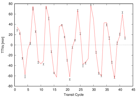
Figure 1: Transit Timing Variations (black dots) computed as the difference between the observed mid-transit times and the linear ephemeris (obtained by fitting a straight line to the mid-transit times series). The red line corresponds to the best dynamical fit corresponding to the solution S1.

Table 3 reports the parameter values corresponding to S1. They were determined from the weighted posteriors calculated by MultiNest. The associated uncertainties are defined by the standard error at the 68.2% confidence level. The orbital elements provided by this solution are astrocentric osculating elements at epoch BJD 55053.2826. The corresponding fit to the TTV signal is shown in Fig. 1.

Table 3: The best-fit parameters and their errors for the solution S1. The first block reports the transit parameters of Kepler-46b obtained from the light-curve analysis. The second block reports the orbital parameters and masses obtained from the dynamical fit. Orbital elements are astrocentric at osculating epoch BJD 55053.2826, the reference plane is the plane at which the impact parameter is 0, and the origin of longitudes is at the line of sight. The third block reports the secondary parameters. $i_{P}$ is the inclination of the planet with respect to the sky plane during transit ($\cos i_{P}\simeq b_{P}R_{\star}/a_{P}$); $I_{p}$ is the inclination of the planetary orbit with respect to the reference plane; $I_{\mathrm{mut}}$ is the mutual inclination relative to the orbital plane of Kepler-46b. The last block lists the stellar parameters compiled from Nesvorný et al. (2012).

	Kepler-46b	Kepler-46c
Transit fit
$R_{P}/R_{\star}$	$0.0887^{+0.0010}_{-0.0012}$
$b_{P}$	$0.757^{+0.022}_{-0.027}$
Dynamical fit
$M_{p}/M_{\star}$ ($\times 10^{-4}$)	$9.372^{+3.941}_{-3.618}$	$3.835^{+0.057}_{-0.055}$
$P_{P}$ (days)	$33.648^{+0.004}_{-0.005}$	$57.325^{+0.116}_{-0.098}$
$e_{P}$	$0.0321^{+0.0069}_{-0.0078}$	$0.0354^{+0.0057}_{-0.0059}$
$b_{P}$	$0.757^{+0.022}_{-0.027}$	$1.483^{+0.418}_{-0.322}$
$\varpi_{P}$ (∘)	$264.2^{+8.2}_{-8.9}$	$294.16^{+8.70}_{-6.42}$
$\lambda_{P}$ (∘)	–	$338.0^{+0.3}_{-0.3}$
$\Omega_{P}$ (∘)	$270$	$261.4^{+22.7}_{-24.3}$
$\delta t$ (d)	$0.0130^{+0.0006}_{-0.0006}$	–
Secondary parameters
$M_{P}$ ($M_{\mathrm{J}}$)	$0.885^{+0.374}_{-0.343}$	$0.362^{+0.016}_{-0.016}$
$a_{P}$ (au)	$0.1971^{+0.0001}_{-0.0001}$	$0.2811^{+0.0003}_{-0.0003}$
$i_{P}$ (∘)	$89.04^{+0.14}_{-0.14}$	$88.66^{+0.26}_{-0.27}$
$I_{P}$ (∘)	$0.957^{+0.028}_{-0.034}$	$1.35^{+0.38}_{-0.29}$
$I_{\mathrm{mut}}$ (∘)	–	$0.43^{+0.40}_{-0.26}$
$R_{P}$ ($R_{\mathrm{J}}$)	$0.810^{+0.035}_{-0.036}$	–
$\rho$ (g cm-3)	$2.069^{+0.913}_{-1.136}$	–
	Kepler-46
Stellar parameters
$M_{\star}$ ($M_{\odot}$)	$0.902^{+0.040}_{-0.038}$
$R_{\star}$ ($R_{\odot}$)	$0.938^{+0.038}_{-0.039}$
$\rho_{\star}$ (g cm-3)	$1.54^{+0.22}_{-0.17}$
$\log g_{\star}$	$4.447^{+0.040}_{-0.035}$
$T_{\mathrm{eff}}$ (K)	$5155^{+150}_{-150}$
$L_{\star}$ ($L_{\odot}$)	$0.556^{+0.078}_{-0.070}$
$M_{V}$	$5.60^{+0.17}_{-0.17}$
Age (Gyr)	$9.7^{+3.7}_{-3.5}$
Distance (pc)	$855^{+68}_{-65}$
[M/H]	$0.41^{+0.10}_{-0.10}$

Table 4: Similar to Table 3 but for the two modes of solution S2.

	Mode 1		Mode 2
	Kepler-46b	Kepler-46c	Kepler-46b	Kepler-46c
Dynamical fit
$M_{p}/M_{\star}$ ($\times 10^{-4}$)	$8.223^{+20.522}_{-6.530}$	$20.151^{+0.930}_{-0.930}$	$7.499^{+19.497}_{-5.875}$	$20.148^{+0.890}_{-0.957}$
$P_{P}$ (d)	$33.609^{+0.002}_{-0.003}$	$81.504^{+0.165}_{-0.501}$	$33.610^{+0.002}_{-0.003}$	$81.520^{+0.152}_{-0.479}$
$e_{P}$	$0.0063^{+0.0047}_{-0.0040}$	$0.0239^{+0.0031}_{-0.0033}$	$0.0067^{+0.0051}_{-0.0042}$	$0.0240^{+0.0032}_{-0.0034}$
$b_{P}$	$0.757$	$4.962^{+1.983}_{-1.153}$	$0.757$	$7.453^{+1.854}_{-1.175}$
$\varpi_{P}$ (∘)	$225.9^{+42.3}_{-108.2}$	$124.1^{+7.8}_{-12.8}$	$229.3^{+38.6}_{-102.3}$	$124.0^{+7.9}_{-13.2}$
$\lambda_{P}$ (∘)	–	$197.2^{+2.6}_{-2.5}$	–	$196.7^{+2.7}_{-2.6}$
$\Omega_{P}$ (∘)	$270$	$19.4^{+8.7}_{-4.5}$	$270$	$207.7^{+7.5}_{-4.1}$
Secondary parameters
$M_{P}$ ($M_{\mathrm{J}}$)	$0.777^{+1.939}_{-0.617}$	$1.904^{+0.121}_{-0.119}$	$0.708^{+1.842}_{-0.562}$	$1.886$
$a_{P}$ (au)	$0.1969^{+0.0001}_{-0.0001}$	$0.3556^{+0.0006}_{-0.0006}$	$0.1969^{+0.0001}_{-0.0001}$	$0.3557^{+0.0006}_{-0.0006}$
$i_{P}$ (∘)	$89.04^{+0.14}_{-0.14}$	$86.51^{+1.85}_{-1.90}$	$89.04^{+0.14}_{-0.14}$	$84.75^{+4.31}_{-4.20}$
$\rho$ (g cm-3)	$1.815^{+4.537}_{-2.042}$	–	$1.655^{+4.310}_{-1.858}$	–

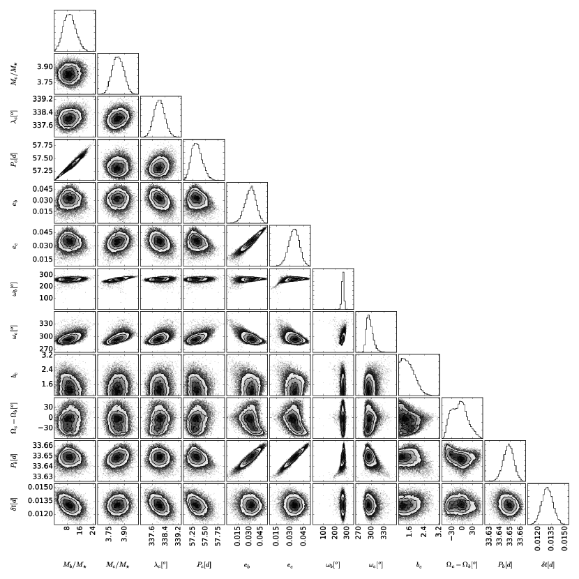
Figure 2: The equally weighted posterior distributions of our 12 model parameters (diagonal), and the corresponding correlations between parameters. The mass ratios are given in units of

The posterior distributions of parameters, and the correlations between pairs of parameters, are shown in Fig. 2. According to solution S1, Kepler-46b is a Jupiter class planet ($M_{b}\simeq 0.9$ $M_{\mathrm{J}}$), with a density similar or slightly higher than that of Jupiter. The companion is a Saturn class planet ($M_{c}\simeq 0.36$ $M_{\mathrm{J}}$) moving on an outer orbit with $P_{c}=57.325$ d.

The period ratio ${P_{c}}/{P_{b}}=1.703$ indicates that the two planets are close to the 5:3 mean motion resonance, but their orbits are not resonant. This configuration may be part of the trend identified previously where compact planetary systems appear to avoid exact resonances (e.g., Veras & Ford 2012). At least in some cases, this can be explained by tidal dissipation acting in the innermost planet (Lithwick & Wu 2012, Batygin & Morbidelli 2013). Kepler-46b, however, is probably too far from its host star for the tidal effects to be important. The orbital eccentricities of the two planets are similar, $e_{b},e_{c}\simeq 0.03$, and the mutual inclination of the orbits is $I_{\mathrm{mut}}=0.43^{\circ}$, confirming the nearly circular and nearly coplanar nature of the planetary system. The small mutual inclination is indicates that Kepler-46c may become a transiting planet in the near future (see Section 4.1).

The second solution (S2) is obtained for the period prior $P_{c}=[80,84]$ days. This solution has a global evidence of $\ln Z_{\mathrm{S2}}=105.97$ and reveals the existence of two modes differing mainly in the mutual inclination between orbits. Specifically, Mode 1 of S2 corresponds to an impact parameter for Kepler-46c of $b_{c}\simeq 5$ with $0^{\circ}\leq\Omega_{c}\leq 180^{\circ}$, while Mode 2 corresponds to $b_{c}\simeq 7$ with $180^{\circ}\leq\Omega_{c}\leq 360^{\circ}$. Mode 1 gives a mutual inclination of $I_{\mathrm{mut}}\simeq 170^{\circ}$ implying that the orbit of Kepler-46c is retrograde, while Mode 2 gives $I_{\mathrm{mut}}\simeq 10^{\circ}$ meaning that both planets are in prograde orbits. The maximum likelihood and reduced $\chi^{2}$ values of the two modes are: $\ln L_{\mathrm{S2}}=157.16$, $\chi^{2}_{\mathrm{S2}}=4.25$ and $\ln L_{\mathrm{S2}}=157.56$, $\chi^{2}_{\mathrm{S2}}=4.21$, respectively. Table 4 summarizes some characteristics of the solution S2.

For both modes, the mass of Kepler-46c would be larger ($M_{c}\simeq 1.9$ $M_{\mathrm{J}}$) than that obtained for the solution S1. The orbital eccentricities of both modes are smaller than for the S1 solution. The orbital period ratio suggested by both modes is ${P_{c}}/{P_{b}}\simeq 2.42$, which places the two planets very close to (but not inside of) the 5:2 mean motion resonance.

Since a $\Delta\chi^{2}\sim 2.25$ between solutions S1 and S2 is not statistically significant enough to penalize any of the solutions, we apply Eq. (A3) to compare the global evidences of S1 and S2. The Bayes factor becomes $\Delta\ln Z=19.26$, suggesting that solution S1 is preferred over S2 with a confidence level of 5.7$\sigma$. This argument can be used to rule out solution S2. It is worth stressing that this conclusion is based on the analysis of the TTVs only, while Nesvorný et al. (2012) had to resort to using the TDV constraints to arrive at the same conclusion.

In order to test how sensitive is the Bayes factor is to the choice of prior distributions, we redo the dynamical fits restricting the intervals of the $e_{b},e_{c}$ priors to $\mathrm{U}[0,\,0.2]$ and the interval of the $P_{c}$ priors to $\mathrm{U}[55,\,84]$. The resulting values of the evidence $\ln Z$ of each solution are higher in this case, as expected from Eq. (A2), but the Bayes factor is almost the same: $\Delta\ln Z=20.81$. This indicates that S1 is still preferred over S2 with a confidence level of 6$\sigma$. Then, we can claim that model selection relying on the Bayes factor is not sensitive to the choice of the priors distributions.

Finally, it is worth noting that if we perform the dynamical fits using more than 35 transits, the solutions do not change significantly. At least three of the five discarded transits (corresponding to cycles 0, 5, and 10; see Sect. 2) allow us to estimate mid-transit times, even with large errors. The dynamical fits using these $35+3$ transits provide again the two solutions S1 and S2, with S2 showing two modes, and the Bayes factor favoring S1. All the parameters of these fits are indistinguishable within 1-$\sigma$ errors with respect to the parameters reported in Tables 3 and 4. We conclude that our two-planet model solution S1 is quite robust.

4.1 Long-term stability

Nesvorný et al. (2012) demonstrated that their S1 solution is dynamically stable over 1 Gyr. Since here we obtained slightly larger values of the orbital eccentricities, slightly smaller values of the mutual inclination, and were able to constrain the mass for Kepler-46b, we find it useful to reanalyze the long-term stability of the system.

We used the orbits and masses corresponding to the solution S1 (see Table 3) and numerically integrated the orbits over 100 Myr using the SWIFT code and a one-day time step. The orbital evolution of the planets in the first 1500 days of this integration is shown in Figs. 3 and 4. The semi-major axes show short-term oscillations with amplitudes never larger than $0.7\%$. Due to the conservation of the total angular momentum, the eccentricities show anti-correlated oscillations with a period of $\simeq 110$ years. We note that, for both planets, these oscillations show amplitudes that are of the same order of the eccentricity uncertainties reported in Table 3. This implies that the eccentricities will be indistinguishable at any epoch, within their 1$\sigma$ uncertainties. The inclinations $I_{P}$ relative to the transit reference plane (see Table 3) also show anti-correlated oscillations with a period of $\simeq 83$ yr resulting from the precession of the nodal longitudes. In this case, the oscillation amplitude of Kepler-46c is also of the same order of the uncertainty in inclination, but for Kepler-46b the amplitude is about five times larger than the uncertainty. The integration results indicate that the orbits show no signs of chaos, and the planetary system is stable at least over 100 Myr.

Our analysis also shows that Kepler-46b should always transit the star, as can be seen from the right panel of Fig. 4. Kepler-46c, on the other hand, is not currently transiting, but it may start to display transits in a few decades. Once it does, Kepler-46 will be a good target for light curve observations that may lead to the confirmation of Kepler-46c and the determination of its radius and density.

5 Conclusion

We reanalyzed the Kepler-46 planetary system using a larger number of transits (35) than in Nesvorný et al. (2012) and applying the Bayesian inference to perform a dynamical fit to the measured TTVs. We obtained two possible solutions, but the Bayesian evidence allows us to rule out one of them without the use of TDVs as in Nesvorný et al. (2012). The availability of a larger number of transits allows us to determine the mass Kepler-46b, and constrain its density.

We confirm that the TTVs signal is well reproduced by a system of two planets on nearly circular and coplanar orbits, with periods of $P_{b}\simeq 33.6$ days and $P_{c}\simeq 57.3$ days, respectively. This means that the two planets are close to, but not inside of, the 5:3 mean motion resonance. With the radius of Kepler-46b determined from the photometric light curve, $R_{b}\simeq 0.85$ $R_{\mathrm{J}}$, and the new mass determination $M_{b}\simeq 0.9$ $M_{\mathrm{J}}$, we can constrain its density to be $\sim 2$ g cm^-3. This indicates, consistently with its Jupiter-like mass, that Kepler-46b has a significant gas component. No density estimate can be inferred for the non-transiting companion Kepler-46c, but the estimated mass $M_{c}\simeq 0.36$ $M_{\mathrm{J}}$ indicates a Saturn-class planet. Interestingly, our new fit indicates that Kepler-46c should start transiting the host star in a few decades.

$10^{-4}$.

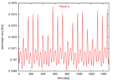
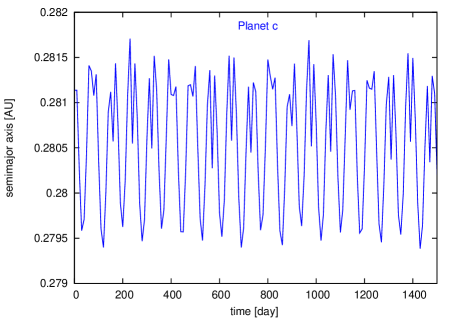
Figure 3: Evolution of the semi-major axes of Kepler-46b (top panel) and Kepler-46c (bottom panel)

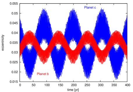
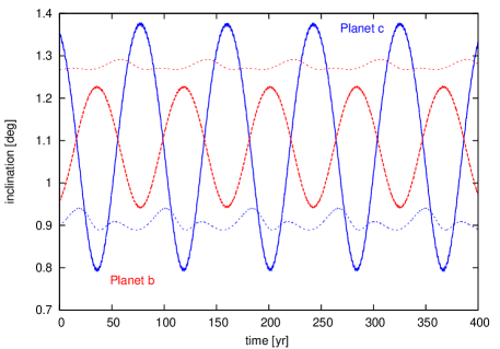
Figure 4: Evolution of the eccentricities (top panel) and inclinations (bottom panel) of Kepler-46b (red full lines) and Kepler-46c (blue full lines) The inclinations are relative to the transit reference plane. The dotted lines in the bottom panel represent the inclination limits below which the planets are expected to show transits (i.e. $b_{P}<1$).

Appendix A Bayesian inference

In order to find the best-fit parameters to the observed mid-transit times, we apply a powerful statistics tool that relies on the Bayes rule:

$$P(\theta|d,M)=\frac{L(d|\theta,M)\pi(\theta,M)}{Z(d|M)}$$ (A1)

This rule gives the posterior distribution $P(\theta|d,M)$ of the parameters $\theta$, for the model $M$, and gives the data $d$, in terms of the likelihood distribution function $L(d|\theta,M)$ within a given set of prior distribution $\pi(\theta,M)$. The expression is normalized by the so-called Bayesian evidence $Z(d|M)$. We recall that in this formula, the prior and the evidence represent probability distributions, while the likelihood is a function that generate the data $d$ given the parameter $\theta$. The prior is the probability of the parameters $\theta$ that is available before making any observation, in other words, it is our state of knowledge of the parameters of the model before considering any new observational data $d$. The evidence is the probability of the data $d$ given the model $M$, integrated over the whole space of parameter $\theta$ as defined by the prior distribution. This is also referred to as the marginal likelihood, and it is given by

$$Z(d|M)=\int{L(d|\theta,M)\pi(\theta,M)}d\theta$$ (A2)

For parameter estimation, the Bayesian evidence simply enters as a normalization constant that can be neglected, as in most cases it seeks to maximum posterior values. However, in the case of having competing models, Bayes rule penalizes them via model selection, and in this case, the Bayesian evidence is relevant. For example, consider two models $M_{1}$ and $M_{2}$; then, the ratio of the posterior probabilities, also known as posterior odds, is given by

$$\frac{P(M_{1}|d)}{P(M_{2}|d)}=\frac{Z(d|M_{1})}{Z(d|M_{2})}\frac{\pi(M_{1})}{\pi(M_{2})}$$ (A3)

Therefore, the posterior odds of the two models is proportional to the ratio of their respective evidences, which is called the Bayes factor. The proportionality becomes an equality when the ratio of the prior probabilities (or prior odds) of the two models is 1.

References

- Agol (2005) Agol, E., Steffen, J., et al. 2005, MNRAS 359, 567
- Ballard (2011) Ballard, S., Fabrycky, D., et al. 2011, ApJ 743, 200
- Batygin (2013) Batygin, K. & Morbidelli, A. 2013, AJ 145, 1
- Borucki (2011) Borucki, W. J., Koch, D. G., et al. 2011, ApJ 736, 19
- Carter (2008) Carter, J. A., Yee, J. C., et al. 2008, ApJ 689, 499
- Dawson (2014) Dawson, R. I., Johnson, J. A., et al. 2014, ApJ 791, 89
- Deck (2014) Deck, K. M., Agol, E., et al. 2014, ApJ 787, 132
- Deck (2015) Deck, K. M. & Agol, E. 2015, ApJ 802, 116
- Feroz (2009) Feroz, F., Hobson, M. P., Bridges, M. 2009, MNRAS 398, 1601
- Feroz (2013) Feroz, F., Hobson, M. P., et al. 2013, arXiv e-print:1306.2144
- Guillot (2015) Guillot, T. & Gautier, D. 2015, in: Treatise on Geophysics, 2nd Edition, G. Schubert (ed.), Elsevier: Amsterdam, p. 529
- Holczer (2016) Holczer, T., Mazeh, T., et al. 2016, ApJS 225, 9
- Holman (2005) Holman, M. J. & Murray, N. W. 2005, Science 307, 1288
- Holman (2010) Holman, M. J., Fabrycky, D. C., et al. 2010, Science 330, 51
- Kipping (2010) Kipping, D. M. 2010, MNRAS 408, 1758
- Kipping (2013a) Kipping, D. M., Hartman, J., et al. 2013, ApJ 770, 101
- Kipping (2013b) Kipping, D. M. 2013, MNRAS 435, 2152
- Levison (1994) Levison, H. F. & Duncan, M. J. 1994, Icarus 108, 18
- Lissauer (2011) Lissauer, J. J., Fabrycky, D. C., et al. 2011, Nature 470, 53
- Lithwick (2012) Lithwick, Y. & Wu, Y. 2012, ApJ 756, L11
- Mandel (2002) Mandel, K. & Algol, E. 2002, ApJ 580, L171
- Mancini (2016) Mancini, L., Lillo-Box, J., et al. 2016, A&A 590, A112
- Miralda (2002) Miralda-Escudé, J. 2002, ApJ 564, 1019
- Nesvorny (2012) Nesvorný, D., Kipping, D. M., et al. 2012, Science 336, 1133
- Nesvorny (2013) Nesvorný, D., Kipping, D. M., et al. 2013, ApJ 777, 3
- Nesvorny (2014) Nesvorný, D., Kipping, D. M., et al. 2014, ApJ 790, 31
- Seager (2003) Seager, S., & Mallén-Ornelas, G., 2003, ApJ 585, 1038
- Steffen (2012) Steffen, J. H., Fabrycky, D. C., et al. 2012, MNRAS 421, 2342
- Teachey (2017) Teachey, A., Kipping, D. M., et al. 2017, ApJ submitted
- Veras (2012) Veras, D. & Ford, E. B. 2012, MNRAS 420, L23
- Xie (2014) Xie, J.-W. 2014, ApJS 210, 25