Doubly Robust Inference for Targeted Minimum Loss Based Estimation in Randomized Trials with Missing Outcome Data

Abstract

Missing outcome data is one of the principal threats to the validity of treatment effect estimates from randomized trials. The outcome distributions of participants with missing and observed data are often different, which increases the risk of bias. Causal inference methods may aid in reducing the bias and improving efficiency by incorporating baseline variables into the analysis. In particular, doubly robust estimators incorporate estimates of two nuisance parameters: the outcome regression and the missingness mechanism (i.e., the probability of missingness conditional on treatment assignment and baseline variables), to adjust for differences in the observed and unobserved groups that can be explained by observed covariates. To obtain consistent estimators of the treatment effect, one of these two nuisance parameters mechanism must be consistently estimated. Such nuisance parameters are traditionally estimated using parametric models, which generally preclude consistent estimation, particularly in moderate to high dimensions. Recent research on missing data has focused on data-adaptive estimation of the nuisance parameters in order to achieve consistency, but the large sample properties of such estimators are poorly understood. In this article we discuss a doubly robust estimator that is consistent and asymptotically normal (CAN) under data-adaptive consistent estimation of the outcome regression or the missingness mechanism. We provide a formula for an asymptotically valid confidence interval under minimal assumptions. We show that our proposed estimator has smaller finite-sample bias compared to standard doubly robust estimators. We present a simulation study demonstrating the enhanced performance of our estimators in terms of bias, efficiency, and coverage of the confidence intervals. We present the results of an illustrative example: a randomized, double-blind phase II/III trial of antiretroviral therapy in HIV-infected persons, and provide R code implementing our proposed estimators.

1 Introduction

Missing data are a frequent problem in randomized trials. If the reasons for outcome missingness and the outcome itself are correlated, unadjusted estimators of the treatment effect are biased, thus invalidating the conclusions of the trial. Most methods to mitigate the bias rely on baseline variables to control for the possible common causes of missingness and the outcome, through estimation of certain “nuisance” parameters, i.e., parameters that are not of interest in themselves, but that are required to estimate the treatment effect. In addition to aiding in correcting bias, methods that use covariate adjustment often provide more precise estimates (see, e.g., Koch et al., 1998; Bang and Robins, 2005; Zhang et al., 2008; Moore and van der Laan, 2009; Colantuoni and Rosenblum, 2015; Díaz et al., 2016). In this article we focus on doubly robust estimators. Doubly robust estimation of treatment effects in randomized trials requires estimation of two possibly high-dimensional nuisance parameters: the outcome expectation within treatment arm conditional on baseline variables (henceforth referred to as outcome regression), and the probability of missingness conditional on baseline variables (henceforth referred to as missingness mechanism).

The large sample properties of doubly robust estimators hinges upon large sample properties of the estimators of the nuisance parameters. In particular: (a) doubly robust estimators remain consistent if at least one of the nuisance parameters is estimated consistently, and (b) the asymptotic distribution of the effect estimator depends on empirical process conditions on the estimators of the nuisance parameters. When parametric models are adopted to estimate the nuisance parameters, a straightforward application of the delta method yields the convergence of the doubly robust estimator to a normal random variable at $n^{1/2}$-rate. The nonparametric bootstrap or an influence function based approach yields consistent estimates of the asymptotic variance and confidence intervals. However, the assumptions encoded in parametric models are rarely justified by scientific knowledge. This implies that parametric models are frequently misspecified, which yields an inconsistent effect estimator. In other words, a doubly robust estimators relying on nuisance parametric models makes no use of the double robustness property (a): it is always inconsistent.

Data-adaptive alternatives to alleviate this shortcoming have been developed over the last decades in the statistics and machine learning literature. These data-adaptive methods offer an opportunity to employ flexible estimators that are more likely to achieve consistency. Methods such as those based on regression trees, regularization, boosting, neural networks, support vector machines, adaptive splines, etc., and ensembles of them offer flexibility in the specification of interactions, non-linear, and higher-order terms, a flexibility that is not available for parametric models. However, the large sample analysis of treatment effects estimates based on machine learning requires hard-to-verify assumptions, and often yield estimators which are not $n^{1/2}$-consistent, and for which no statistical inference (i.e., p-values and confidence intervals) is available. Nonetheless, data-adaptive estimation has been widely used in estimation of causal effects from observational data (a few examples include van der Laan et al., 2005; van der Laan, 2006; Ridgeway and McCaffrey, 2007; Bembom et al., 2008; Lee et al., 2010; Neugebauer et al., 2016). Indeed, the statistics field of targeted learning (see e.g., van der Laan and Rubin, 2006; van der Laan and Rose, 2011; van der Laan and Starmans, 2014) is concerned with the development of optimal ($n^{1/2}$-consistent, asymptotically normal, efficient) estimators of smooth low-dimensional parameters through the use state-of-the art machine learning.

We develop estimators for analyzing data from randomized trials with missing outcomes, when the missingness probabilities and the outcome regression are estimated with data-adaptive methods. We propose two estimators: an augmented inverse probability weighted estimator (AIPW), and a targeted minimum loss based estimator (TMLE). Our methods are inspired by recent work by van der Laan (2014); Benkeser et al. (2016), who developed an estimator of the mean of an outcome from incomplete data when data-adaptive estimators are used for the missingness mechanism. In addition to extending their methodology to our problem, our main contribution is to simplify the assumptions of their theorems to two conditions: consistent estimation of at least one of the nuisance parameters, and a condition restricting the class of estimators of the nuisance parameters to Donsker classes (those for which a uniform central limit theorem applies). Though the Donsker condition may be removed through the use of a cross-validated version of our TMLE, the results are straightforward extensions of the work of Zheng and van der Laan (2011), and we do not pursue such results here. We show that the doubly robust asymptotic distribution of these novel estimators requires a slightly stronger version of the standard double robustness in which the nuisance parameters converge to their (possibly misspecified) limits at $n^{1/4}$-rate, with at least one of them converging to the correct limit. Specifically, we show that the TMLE is CAN under these empirical process conditions, and provide its influence function. This allows the construction of Wald-type confidence intervals under the assumption that at least one of the nuisance parameters is consistently estimated, though it is not necessary to know which one. We also make connections between the proposed estimators and standard $M$-estimation theory, by noting that our estimators (and those of van der Laan, 2014; Benkeser et al., 2016) amount to controlling the behavior of the “drift” term resulting from the analysis of the estimator’s empirical process. Thus, our methods and theory may be used to improve the performance of other $M$-estimators in causal inference and missing data problems. The need to control the behavior of such terms has been previously recognized in the semiparametric estimation literature, for example in Theorem 5.31 of van der Vaart (1998) (see also Section 6.6 of Bolthausen et al., 2002).

In related work, Vermeulen and Vansteelandt (2015, 2016) recently proposed estimators that also target minimization of the drift term. However, their methods are not suitable for our application because they rely on parametric working models for the missingness mechanism. Since we do not know the functional form of the missingness mechanism, we must resort to data-adaptive methods to estimate this probability.

The paper is organized as follows. In Section 2 we discuss our illustrative application and define the statistical estimation problem. In Section  3 we present estimators from existing work; in Section 4 we discuss possible ways of repairing the AIPW, and show that such repairs do not help us achieve desirable properties such as asymptotic linearity. In Section 5 we present our proposed TML estimator an show that it is asymptotically normal with known doubly robust asymptotic distribution, where the latter concept means that the distribution is known under consistent estimation of at least one nuisance parameter. Simulation studies are presented in Section 6. These simulation studies demonstrate that our estimators can lead to substantial bias reduction, as well as improved coverage of the Wald-type confidence intervals. Section 7 presents some concluding remarks and directions of future research.

2 Illustrative Application

We illustrate our methods in the analysis of data from the ACTG 175 study (Hammer et al., 1996). ACTG 175 was a randomized clinical trial in which 2139 adults infected with the human immunodeficiency virus type I, whose CD4 T-cell counts were between 200 and 500 per cubic millimeter, were randomized to compare four antiretroviral therapies: zidovudine (ZDV) alone, ZDV+didanosine(ddI), ZDV+zalcitabine(ddC), and ddI alone.

One goal of the study was to compare the four treatment arms in terms of the CD4 counts at week 96 after randomization. By week 96, 797 (37.2%) subjects had dropped out of the study. Dropout rates varied between 35.7-39.6% across treatment arms. The investigators found dropout to be associated to patient characteristics such as ethnicity and history of injection-drug use, which are also associated with the outcome, therefore causing informative missingness. Other baseline variables collected at the beginning of the study include age, gender, weight, CD4 count, hemophilia, homosexual activity, the Karnofsky score, and prior antiretroviral therapy.

2.1 Observed Data and Notation

Let $W$ denote a vector of observed baseline variables, let $A$ denote a binary treatment arm indicator (e.g., in our application we have four such indicators). Let $Y$ denote the outcome of interest, observed only when a missingness indicator $M$ is equal to one. Throughout, we assume without loss of generality that $Y$ takes values on $[0,1]$. We use the word model in the classical statistical sense to refer to a set of probability distributions for the observed data $O=(W,A,M,MY)$. We assume that the true distribution of $O$, denoted by $P_{0}$, is an element of the nonparametric model, denoted by $\cal M$, and defined as the set of all distributions of $O$ dominated by a measure of interest $\nu$. The word estimator is used to refer to a particular procedure or method for obtaining estimates of $P_{0}$ or functionals of it. Assume we observe an i.i.d. sample $O_{1},\ldots,O_{n}$, and denote its empirical distribution by $\mathbb{P}_{n}$. For a general distribution $P$ and a function $f$, we use $Pf$ to denote $\int f(o)dP(o)$. We use $m(w)$ to denote $E(Y\mid M=1,A=1,W=w)$, $g_{A}(w)$ to denote $P(A=a\mid W=w)$, and $g_{M}(w)$ to denote $P(M=1\mid A=1,W=w)$. The index naught is added when the expectation and probabilities are computed under $P_{0}$ (i.e., $m_{0}$, $g_{A,0}$, and $g_{M,0}$). We define $g(w)=g_{A}(w)g_{M}(w)$.

2.2 Treatment Effect in Terms of Potential Outcomes and Identification

Define the potential outcome $Y_{1}$ as the outcome that would have been observed had study arm $A=1$ and missingness $M=1$ been externally set with probability one. The target estimand is defined as $\theta_{\mbox{\footnotesize causal}}=E(Y_{1})$. The index “causal” denotes a parameter of the distribution of the potential outcome $Y_{1}$. We show that $\theta_{\mbox{\footnotesize causal}}$ can be equivalently expressed as a parameter $\theta$ of the observed data distribution $P_{0}(W,A,M,MY)$, under Assumption 1-4 below. This is useful since the potential outcome is not observed, in contrast to the data vector $(W,A,M,MY)$, which we can make inferences about. Define the following assumptions:

Assumption 1Consistency.

$Y=M\{AY_{1}+(1-A)Y_{0}\}$,

Assumption 2Randomization.

$A$ is independent of $Y_{1}$ conditional on $W$,

Assumption 3Missing at random.

$M$ is independent of $Y_{1}$ conditional on $(A,W)$,

Assumption 4Positivity.

$g(w)>0$ with probability one over draws of $W$.

Assumption 1 connects the potential outcomes to the observed outcome. Assumption 2 holds by design in a randomized trial such as our illustrative example. Assumption 3, which is similar to that in Rubin (1987), means that missingness is random within strata of treatment and baseline variables (which is often abbreviated as “missing at random”, or MAR). Equivalently, the MAR assumption may be interpreted as the assumption that all common causes of missingness and the outcome are observed and form part of the vector of baseline variables $W$. Assumption 4 guarantees that $m_{0}$ is well defined.

Under Assumption 1-4 above, our target estimand $\theta_{\mbox{\footnotesize causal}}$ is identified as $\theta_{0}=E_{P_{0}}\{m_{0}(W)\}.$ Note that this parameter definition allows us to compute the parameter value at any distribution $P$ in the model $\mathcal{M}$. According to this observation, we use the notation $\theta(P)=E_{P}\{m(W)\}$, where $\theta_{0}=\theta(P_{0})$.

2.3 Data Analysis

We present the results of applying our estimators to the ACTG data. To estimate the probability of missingness conditional on baseline variables $g_{M}$, we fit an ensemble predictor known as super learning (van der Laan et al., 2007; Polley et al., 2016) to the missingness indicator in each treatment arm. Super learning builds a convex combination of predictors in a user-given library, where the combination weights are chosen such that the cross-validated prediction risk is minimized. For predicting probabilities, we define the prediction risk as the average of the negative log-likelihood of a Bernoulli variable. The algorithms used in the ensemble along with their weights are presented in Table 1. Note that the algorithms that more accurately predict missingness are data-adaptive algorithms with flexible functional forms, or algorithms that incorporate some type of variable selection.

	Treatment arm
Algorithm	ZVD	ZVD+ddI	ZVD+ddC	ddI
GLM	0.00	0.00	0.00	0.00
Lasso	0.02	0.21	0.00	0.85
Bayes GLM	0.21	0.38	0.19	0.00
GAM	0.00	0.00	0.02	0.00
MARS	0.78	0.38	0.30	0.15
Random Forest	0.00	0.03	0.49	0.00

Table 1: Coefficients in the super learner convex combination for predicting 96 week dropout.

We also use the super learner to estimate the expected CD4 T-cell count at 96 weeks after randomization among subjects still in the study, conditional on covariates. The prediction risk in this case is defined as the average of the squared prediction residuals. The results are presented in Table 2. For the outcome regression, the best predictive algorithms are also data-adaptive.

	Treatment arm
Algorithm	ZVD	ZVD+ddI	ZVD+ddC	ddI
GLM	0.00	0.00	0.00	0.00
Lasso	1.00	0.30	0.08	0.60
Bayes GLM	0.00	0.02	0.00	0.00
GAM	0.00	0.00	0.60	0.34
MARS	0.00	0.00	0.00	0.06
Random Forest	0.00	0.68	0.32	0.00

Table 2: Coefficients in the super learner convex combination for predicting CD4 T-cell count.

The results in Tables 1 and 2 highlight the need to use data-adaptive estimators for the nuisance parameters in the construction of a doubly robust estimator for $\theta_{0}$. As we show below in Section 3, standard doubly robust estimators are not guaranteed to have desirable properties such as $n^{1/2}$-consistency and doubly robust asymptotic linearity when such data-adaptive estimators are used. This motivates the construction of the estimators we propose.

Figure 1 shows the estimated CD4 T-cell count for each treatment arm according to several estimators, along with their corresponding 95% confidence intervals. The targeted maximum likelihood estimator (TMLE van der Laan and Rose, 2011) and the augmented inverse-probability weighted estimator (AIPW) are standard doubly robust estimators, whereas DTMLE and DAIPW are the modifications described in Section 4 below. Unlike the TMLE and AIPW, the confidence intervals of the DTMLE is expected to have correct asymptotic coverage under consistent estimation of at least one nuisance parameter (Theorem 2). Unfortunately, the same claim does not seem to hold for the DAIPW, although we expect this estimator to have similar properties to the DTMLE in finite samples. For reference, we also present the unadjusted estimate obtained by computing the empirical mean of the outcome within each treatment arm among subjects with observed outcomes.

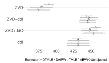
Figure 1: Estimated CD4 T-cell count on week 96 in each treatment arm, according to several estimators, along with confidence intervals.

The dataset is available in the R package speff2trial (Juraska et al., 2012), the super learner predictor was computed using the package SuperLearner (Polley et al., 2016). R code to compute these estimators is given in Appendix B.

3 Existing Estimators from the Semiparametric Efficiency Literature

We start by presenting the efficient influence function for estimation of $\theta_{0}$ in model $\cal M$ (see Hahn, 1998):

$$D_{\eta,\theta}(O)=\frac{A\,M}{g(W)}\{Y-m(W)\}+m(W)-\theta,$$ (1)

where we have denoted $\eta=(g,m)$. The efficient influence function $D_{\eta,\theta}$ is a fundamental object for the analysis and construction of estimators of $\theta_{0}$ in the non-parametric model $\mathcal{M}$. First, it is a doubly robust estimating function, i.e., for given estimators $\hat{m}$ and $\hat{g}$ of $m_{0}$ and $g_{0}$, respectively, an estimator that solves for $\theta$ in the following estimating equation is consistent if at least one of $m_{0}$ or $g_{0}$ is estimated consistently (while the other converges to a limit that may be incorrect, see Theorem 5.9 of van der Vaart, 1998):

$$\sum_{i=1}^{n}\frac{A_{i}\,M_{i}}{\hat{g}(W_{i})}\{Y_{i}-\hat{m}(W_{i})\}+\sum_{i=1}^{n}\left\{\hat{m}(W_{i})-\theta\right\}=0.$$ (2)

The estimator constructed by directly solving for $\theta$ in the above equation is often referred to as the augmented IPW estimator, and we denote it by $\hat{\theta}_{\operatorname{aipw}}$. Second, the efficient influence function (1) characterizes the efficiency bound for estimation of $\theta_{0}$ in the model $\mathcal{M}$. Specifically, under consistent estimation of $m_{0}$ and $g_{0}$ at a fast enough rate (which we define below), an estimator that solves (2) has variance smaller or equal to that of any regular, asymptotically linear estimator of $\theta_{0}$ in $\mathcal{M}$. This property is sometimes called local efficiency.

The augmented IPW has been criticized because directly solving the estimating equation (2) may drive the estimate out of bounds of the parameter space (see e.g., Gruber and van der Laan, 2010), which may lead to poor performance in finite samples. Alternatives to repair the AIPW have been discussed by Kang and Schafer (2007); Robins et al. (2007); Tan (2010). One such approach consists in solving the estimating equation (2) with the first term in the left hand side divided by the empirical mean of the weights $A\,M/\hat{g}(W)$. Alternatively, the targeted minimum loss based estimation (TMLE) approach of van der Laan and Rubin (2006); van der Laan and Rose (2011) provides a more principled method to construct estimators that stay within natural bounds of the parameter space, for any smooth parameter.

The TMLE of $\theta_{0}$ is defined as a substitution estimator $\hat{\theta}_{\operatorname{tmle}}=\theta(\tilde{P})$, where $\tilde{P}$ is an estimate of $P_{0}$ constructed such that the corresponding $\tilde{\eta}$ and $\theta(\tilde{P})$ solve the estimating equation $\sum_{i=1}^{n}D_{\tilde{\eta},\theta(\tilde{P})}(O_{i})=0$. The estimator $\tilde{P}$ is constructed by tilting an initial estimate $\hat{P}$ towards a solution of the relevant estimating equation, by means of a maximum likelihood estimator in a parametric submodel.

Specifically, a TMLE may be constructed by fitting the logistic regression model

$$\operatorname{logit}m_{\epsilon}(w)=\operatorname{logit}\hat{m}(w)+\epsilon\frac{1}{\hat{g}(w)},$$ (3)

among observations with $(A_{i},M_{i})=(1,1)$. Here $\operatorname{logit}(p)=\log\{p(1-p)^{-1}\}$. In this expression $\epsilon$ is the parameter of the model, $\operatorname{logit}\hat{m}(w)$ is an offset variable, and the initial estimates $\hat{m}$ and $\hat{g}$ are treated as fixed. The parameter $\epsilon$ is estimated using the empirical risk minimizer

$$\hat{\epsilon}=\arg\max_{\epsilon}\sum_{i=1}^{n}A_{i}M_{i}\{Y_{i}\log m_{\epsilon}(W_{i})+(1-Y_{i})\log(1-m_{\epsilon}(W_{i}))\}.$$

The tilted estimator of $m_{0}(w)$ is defined as $\tilde{m}(w)=m_{\hat{\epsilon}}(w)=\operatorname{expit}\{\operatorname{logit}\hat{m}(w)+\hat{\epsilon}/\hat{g}(w)\}$, where $\operatorname{expit}(x)=\operatorname{logit}^{-1}(x)$, and the TMLE of $\theta_{0}$ is defined as

$$\hat{\theta}_{\operatorname{tmle}}=\frac{1}{n}\sum_{i=1}^{n}\tilde{m}(W_{i}).$$

Because the empirical risk minimizer of model (3) solves the score equation

$$\sum_{i=1}^{n}\frac{A_{i}\,M_{i}}{\hat{g}(W_{i})}\{Y_{i}-m_{\hat{\epsilon}}(W_{i})\}=0,$$

it follows that $\sum_{i=1}^{n}D_{\tilde{\eta},\hat{\theta}_{\operatorname{tmle}}}(O_{i})=0$ with $\tilde{\eta}=(\tilde{g},\tilde{m})$. Since this procedure does not update the estimator $\hat{g}$, we have $\tilde{g}=\hat{g}$.

Further discussion on the construction of the above TMLE may be found in Gruber and van der Laan (2010). Porter et al. (2011) provides an excellent review of other doubly robust estimators along with a discussion of their strengths and weaknesses. In this article we focus on the estimators $\hat{\theta}_{\operatorname{aipw}}$ and $\hat{\theta}_{\operatorname{tmle}}$ defined above, but our methods can be used to construct enhanced versions of other doubly robust estimators.

3.1 Analysis of Asymptotic Properties of Doubly Robust Estimators

The analysis of the asymptotic properties of the AIPW (as well as the TMLE or any other estimator that solves the estimating equation (2)) may be based on standard $M$-estimation and empirical process theory. Here we focus on an analysis of the AIPW based on the asymptotic theory presented in Chapter 5 of van der Vaart (1998).

Define the following conditions:

Condition 1Doubly robust consistency.

Let $||\cdot||$ denote the $L_{2}(P_{0})$ norm defined as $||f||^{2}=\int f^{2}dP_{0}$. Assume

1. There exists $\eta_{1}=(g_{1},m_{1})$ with either $g_{1}=g_{0}$ or $m_{1}=m_{0}$ such that $||\hat{m}-m_{1}||=o_{P}(1)$ and $||\hat{g}-g_{1}||=o_{P}(1)$.

2. For $\eta_{1}$ as above, $||\hat{m}-m_{1}||\,||\hat{g}-g_{1}||=o_{P}(n^{-1/2})$.

Condition 2Donsker.

Let $\eta_{1}$ be as in Condition 1-(i). Assume the class of functions $\{\eta=(g,m):||m-m_{1}||<\delta,||g-g_{1}||<\delta\}$ is Donsker for some $\delta>0$.

Under Condition 1-(i) and 2, a straightforward application of Theorems 5.9 and 5.31 of van der Vaart (1998) (see also example 2.10.10 of van der Vaart and Wellner, 1996) yields

$$\hat{\theta}_{\operatorname{aipw}}-\theta_{0}=\beta(\hat{\eta})+(\mathbb{P}_{n}-P_{0})D_{\eta_{1},\theta_{0}}+o_{P}\big{(}n^{-1/2}+|\beta(\hat{\eta})|\big{)},$$ (4)

where $\beta(\hat{\eta})=P_{0}D_{\hat{\eta},\theta_{0}}$. Thus, the probability distribution of doubly robust estimators depends on $\hat{\eta}$ through the “drift” term $\beta(\hat{\eta})$. For our parameter $\theta$ the drift term is given by

$$\beta(\hat{\eta})=\int\frac{1}{\hat{g}}(\hat{g}-g_{0})(\hat{m}-m_{0})dP_{0}.$$ (5)

Note that under Condition 1, $\beta(\hat{\eta})$ converges to zero in probability so that $\hat{\theta}_{\operatorname{aipw}}$ and $\hat{\theta}_{\operatorname{tmle}}$ are consistent. Efficiency under $\eta_{1}=\eta_{0}$ can be proved as follows. The Cauchy-Schwartz inequality shows that

$$\beta(\hat{\eta})\leq C||\hat{m}-m_{0}||\,||\hat{g}-g_{0}||,$$

for some constant $C$. Under Condition 1 and $\eta_{1}=\eta_{0}$, we get $\beta(\hat{\eta})=o_{P}(n^{-1/2})$ so that (4) yields

$$\hat{\theta}_{\operatorname{aipw}}-\theta_{0}=(\mathbb{P}_{n}-P_{0})D_{\eta_{0},\theta_{0}}+o_{P}\big{(}n^{-1/2}\big{)}.$$

An identical result holds replacing $\hat{\theta}_{\operatorname{aipw}}$ by $\hat{\theta}_{\operatorname{tmle}}$ in the above display. Asymptotic normality and efficiency follows from the central limit theorem.

In the more common doubly robust scenario in which at most one of $m_{0}$ or $g_{0}$ is consistently estimated, the large sample analysis of doubly robust estimators relies on the assumption that $\beta(\tilde{\eta})$ is asymptotically linear (see Appendix 18 of van der Laan and Rose, 2011). If $\hat{\eta}$ is estimated in a parametric model, the delta method yields the required asymptotic linearity. However, this assumption is hard to verify when $\hat{\eta}$ uses data-adaptive estimators; in fact there is no reason to expect that it would hold in general.

In the remainder of the paper we construct drift-corrected estimators $\hat{\theta}_{\operatorname{daipw}}$ and $\hat{\theta}_{\operatorname{dtmle}}$ that control the asymptotic behavior through estimation of the drift term in the more plausible doubly robust situation where either $g_{1}=g_{0}$ or $m_{1}=m_{0}$, but not necessarily both.

Remark 1 (Asymptotic bias of the AIPW and TMLE under double inconsistency).

Assume $\hat{\eta}=(\hat{g},\hat{\eta})$ converges to some $\eta_{1}=(g_{1},m_{1})$. Define $\theta_{1}=P_{0}m_{1}$, and note that $D_{\eta_{1},\theta_{1}}=D_{\eta_{1},\theta_{0}}-\theta_{1}+\theta_{0}$. Under Condition 2, an application of Theorem 5.31 of van der Vaart (1998) yields

$$\hat{\theta}_{\operatorname{aipw}}-\theta_{1}=\beta(\hat{\eta})+(\mathbb{P}_{n}-P_{0})D_{\eta_{1},\theta_{1}}+o_{P}\big{(}n^{-1/2}+|\beta(\hat{\eta})|\big{)}.$$

Substituting $D_{\eta_{1},\theta_{1}}=D_{\eta_{1},\theta_{0}}-\theta_{1}+\theta_{0}$ yields

$$\hat{\theta}_{\operatorname{aipw}}-\theta_{0}=\beta(\hat{\eta})+(\mathbb{P}_{n}-P_{0})D_{\eta_{1},\theta_{0}}+o_{P}\big{(}n^{-1/2}+|\beta(\hat{\eta})|\big{)}.$$

The above expression also holds for $\hat{\theta}_{\operatorname{aipw}}$ replaced with $\hat{\theta}_{\operatorname{tmle}}$ and $\hat{\eta}$ replaced with $\tilde{\eta}$. The empirical process term $(\mathbb{P}_{n}-P_{0})D_{\eta_{1},\theta_{0}}$ has mean zero. Thus, controlling the magnitude of $\beta(\hat{\eta})$ and $\beta(\tilde{\eta})$ is expected to reduce the bias of $\hat{\theta}_{\operatorname{aipw}}$ and $\hat{\theta}_{\operatorname{tmle}}$, respectively, in the double inconsistency case in which $m_{1}\neq m_{0}$ and $g_{1}\neq g_{0}$.

4 Repairing the AIPW Estimator Through Estimation of $\beta(\hat{\eta})$

As seen from the analysis of the previous section, the consistency Condition 1 with $\eta_{1}=\eta_{0}$ is key in proving the optimality ($n^{1/2}$-consistency, asymptotic normality, efficiency) of doubly robust estimators such as the TMLE and the AIPW. The asymptotic distribution of doubly robust estimators under violations of this condition depends on the behavior of the drift term $\beta(\hat{\eta})$. We propose a method that controls the asymptotic behavior of $\beta(\hat{\eta})$. This is achieved through a decomposition into score functions associated to estimation of $m_{0}$ and $g_{0}$. In light of Remark 1 controlling the magnitude and variation of $\beta(\hat{\eta})$ is also important to reduce the bias of the TMLE when either $g_{0}$ or $m_{0}$ are inconsistently estimated.

We introduce the following strengthened doubly robust consistency condition:

Condition 3Strengthened doubly robust consistency.

$\hat{\eta}=(\hat{g},\hat{\eta})$ converges to some $\eta_{1}=(g_{1},m_{1})$ in the sense that $||\hat{m}-m_{1}||=o_{P}(n^{-1/4})$ and $||\hat{g}-g_{1}||=o_{P}(n^{-1/4})$ with either $g_{1}=g_{0}$ or $m_{1}=m_{0}$.

The following lemma provides an approximation for the drift term in terms of score function in the tangent space of each of the models for $g_{0}$ and $m_{0}$. Such approximation is achieved through the definition of the following univariate regression functions:

$$\gamma_{A,0}(W) =P_{0}\big{\{}A=1\mid m_{1}(W)\big{\}},$$

$$\gamma_{M,0}(W) =P_{0}\big{\{}M=1\mid A=1,m_{1}(W)\big{\}},$$

$$r_{A,0}(W) =E_{P_{0}}\left\{\frac{A-g_{A,1}(W)}{g_{A,1}(W)}\mathrel{\bigg{|}}m_{1}(W)\right\},$$ (6)

$$r_{M,0}(W) =E_{P_{0}}\left\{\frac{M-g_{M,1}(W)}{g_{1}(W)}\mathrel{\bigg{|}}A=1,m_{1}(W)\right\},$$

$$e_{0}(W) =E_{P_{0}}\big{\{}Y-m_{1}(W)\mid A=1,M=1,g_{1}(W)\big{\}}.$$

Note that the residual regressions $r_{A,0}$, $r_{M,0}$, and $e_{0}$ are equal to zero if the limits $g_{A,1}$, $g_{M,1}$, and $m_{1}$ of the nuisance estimators are correct. To see this, it suffices to replace $g_{A,0}$ for $g_{A,1}$ in $r_{A,0}$, and apply the iterated expectation rule conditioning first on $W$.

Theorem 1 (Asymptotic approximation of the drift term).

Denote $\lambda_{0}=(\gamma_{A,0},\gamma_{M,0},r_{A,0},r_{M,0},e_{0})$, and define the following score functions:

$$D_{Y,\hat{m},\lambda_{0}}(O) =A\,M\left\{\frac{r_{A,0}(W)}{\gamma_{A,0}(W)}+\frac{r_{M,0}(W)}{\gamma_{0}(W)}\right\}\{Y-\hat{m}(W)\}$$

$$D_{M,\hat{g},\lambda_{0}}(O) =\frac{A\,e_{0}(W)}{\hat{g}(W)}\{M-\hat{g}_{M}(W)\}$$

$$D_{A,\hat{g},\lambda_{0}}(O) =\frac{e_{0}(W)}{\hat{g}_{A}(W)}\{A-\hat{g}_{A}(W)\},$$

where $\gamma_{0}(w)=\gamma_{A,0}(w)\gamma_{M,0}(w)$. Under Condition 3 we have $\beta(\hat{\eta})=P_{0}\{D_{A,\hat{g},\lambda_{0}}+D_{M,\hat{g},\lambda_{0}}+D_{Y,\hat{m},\lambda_{0}}\}+o_{P}(n^{-1/2})$.

Unlike expression 5, the above approximation of the drift depends only on one-dimensional nuisance parameters which are easily estimable through non-parametric smoothing techniques. These one-dimensional parameters are functions of the possibly misspecified limits of your estimators. However, in what follows this does not prove to be problematic. In particular, $\beta(\hat{\eta})$ may be estimated as follows. First, we construct an estimator of $\lambda_{0}$ component-wise by fitting non-parametric regression estimators. Since all the regression functions in (6) are one-dimensional, they may be estimated by fitting a kernel regression. For instance, for a second-order kernel function $K_{h}$ with bandwidth $h$ the estimator of $e_{0}$ is given by

$$\hat{e}(w)=\frac{\sum_{i=1}^{n}A_{i}\,M_{i}\,K_{\hat{h}}\{\hat{g}(W_{i})-\hat{g}(w)\}\{Y_{i}-\hat{m}(W_{i})\}}{\sum_{i=1}^{n}A_{i}\,M_{i}\,K_{\hat{h}}\{\hat{g}(W_{i})-\hat{g}(w)\}}.$$ (7)

The bandwidth is chosen as $\hat{h}=n^{-0.1}\hat{h}_{\operatorname{opt}}$, where $\hat{h}_{\operatorname{opt}}$ is the optimal bandwidth chosen using K-fold cross-validation (the optimality of this selector is discussed in van der Vaart et al., 2006). This bandwidth yields a convergence rate that allows application of uniform central limit theorems (see Theorems 4 and 5 of Giné and Nickl, 2008).

An estimator of the drift term may be constructed as

$$\hat{\beta}(\hat{\eta})=\frac{1}{n}\sum_{i=1}^{n}\left[\frac{\hat{e}(W_{i})}{\hat{g}_{A}(W_{i})}\{A_{i}-\hat{g}_{A}(W_{i})\}+\frac{A_{i}\,\hat{e}(W_{i})}{\hat{g}(W_{i})}\{M_{i}-\hat{g}_{M}(W_{i})\}+\right.\\ \left.A_{i}M_{i}\left\{\frac{\hat{r}_{A}(W_{i})}{\hat{\gamma}(W_{i})}+\frac{\hat{r}_{M}(W_{i})}{\hat{\gamma}_{M}(W_{i})}\right\}\{Y_{i}-\hat{m}(W_{i})\}\right].$$ (8)

In light of equation (4), the above estimator may be subtracted from the AIPW (or the TMLE) to obtain a drift-corrected estimator. We denote this estimator by $\hat{\theta}_{\operatorname{daipw}}=\hat{\theta}_{\operatorname{aipw}}-\hat{\beta}(\hat{\eta})$.

Though sensible in principle, $\hat{\theta}_{\operatorname{daipw}}$ suffers from drawbacks similar to the standard AIPW estimator $\hat{\theta}_{\operatorname{aipw}}$: it may yield an estimator out of bounds of the parameter space and therefore have suboptimal finite sample performance (we illustrate this in our simulation study in Section 6). In addition, a large sample analysis of $\hat{\theta}_{\operatorname{daipw}}$ suggests that the $n^{1/2}$-consistency of $\hat{\theta}_{\operatorname{daipw}}$ requires consistent estimation of $\lambda_{0}$ at the $n^{1/2}$ parametric rate. In particular, under Condition 1-2, equation (4) yields

$$\hat{\theta}_{\operatorname{daipw}}-\theta_{0}=\beta(\hat{\eta})-\hat{\beta}(\hat{\eta})+(\mathbb{P}_{n}-P_{0})D_{\eta_{1},\theta_{0}}+o_{P}\big{(}n^{-1/2}+|\beta(\hat{\eta})|\big{)}.$$ (9)

Lemma 1 in the appendix shows that, under Condition 3,

$$\beta(\hat{\eta})-\hat{\beta}(\hat{\eta})=-(\mathbb{P}_{n}-P_{0})\{D_{A,\hat{g},\lambda_{0}}+D_{M,\hat{g},\lambda_{0}}+D_{Y,\hat{m},\lambda_{0}}\}+o_{P}(n^{-1/2}).$$ (10)

Asymptotic linearity of $\hat{\theta}_{\operatorname{daipw}}$ would then require that $|\beta(\hat{\eta})|=O_{P}(n^{-1/2})$, so that the last term in the right-hand side of expression (9) is $o_{P}(n^{-1/2})$. This would require $\lambda_{0}$ to be estimated at rate $n^{1/2}$, which is in general not achievable in the non-parametric model (e.g., the convergence rate of a kernel regression estimator with second order kernel and optimal bandwidth is $n^{2/5}$). It would thus appear that the $\hat{\theta}_{\operatorname{daipw}}$ estimator will not generally be asymptotically linear if the estimator of $\lambda_{0}$ converges to zero more slowly than $n^{-1/2}$.

Surprisingly, the large-sample analysis of the $\hat{\theta}_{\operatorname{dtmle}}$ counterpart presented in Section 5 below requires slower convergence rates for the estimator of $\lambda_{0}$, such that a Kernel regression estimator provides a sufficiently fast rate. This fact has been previously noticed in the context of estimation of a counterfactual mean by Benkeser et al. (2016). We note that the optimal bandwidth $\hat{h}_{\text{opt}}$ in estimation of $\lambda_{0}$ yields estimators for which uniform central limit theorems do not apply. Therefore we propose to undersmooth using the bandwidth $\hat{h}$.

5 Targeted Maximum Likelihood Estimation with Doubly Robust Inference

As transpires from the developments of the previous section, it is necessary to construct estimators $\hat{\eta}$ such that $\beta(\hat{\eta})$ is $O_{P}(n^{-1/2})$. In light of expression (10), this can be achieved through the construction of an estimator $\tilde{\eta}$ that satisfies $\hat{\beta}(\tilde{\eta})=0$. This construction is based on the fact that $D_{Y,\hat{m},\lambda_{0}}$, $D_{M,\hat{g},\lambda_{0}}$, and $D_{M,\hat{g},\lambda_{0}}$ are score equations in the model for $m_{0}$, $g_{M,0}$, and $g_{A,0}$, respectively. As a result, adding the corresponding covariates to a logistic tilting model will tilt an initial estimator $\hat{\eta}=(\hat{g},\hat{m})$ towards a solution $\tilde{\eta}$ of the bias-reducing estimating equations $\hat{\beta}(\tilde{\eta})=0$, in a similar way to the logistic tilting submodel (3).

The proposed drift-corrected TMLE is defined by the following algorithm:

1. Initial estimators. Obtain initial estimators $\hat{g}_{A}$, $\hat{g}_{M}$, and $\hat{m}$ of $g_{A,0}$, $g_{M,0}$, and $m_{0}$. These estimators may be based on data-adaptive predictive methods that allow flexibility in the specification of the corresponding functional forms. Construct estimators $\hat{\gamma}_{A}$, $\hat{\gamma}_{M}$, $\hat{\mu}$ of $\gamma_{A,0}$, $\gamma_{M,0}$, $\mu_{0}$, respectively, by fitting kernel regression estimators as described in the previous subsection.

2. Compute auxiliary covariates. For each subject, compute the auxiliary covariates

   $$W_{1}(w)=\frac{1}{\hat{g}(w)},\,W_{2}(w)=\frac{\hat{r}_{A}(w)}{\hat{\gamma}(w)}+\frac{\hat{r}_{M}(w)}{\hat{\gamma}_{M}(w)},\,Z_{A}(w)=\frac{\hat{e}(w)}{\hat{g}_{A}(w)},\,Z_{M}(w)=\frac{\hat{e}(w)}{\hat{g}(w)}$$

3. Solve estimating equations. Estimate the parameter $\epsilon=(\epsilon_{A},\epsilon_{M},\epsilon_{Y,1},\epsilon_{Y,2})$ in the logistic tilting models

   $$\operatorname{logit}m_{\epsilon}(w) =\operatorname{logit}\hat{m}(w)+\epsilon_{Y,1}W_{1}(w)+\epsilon_{Y,2}W_{2}(w),$$ (11)

   $$\operatorname{logit}g_{M,\epsilon}(w) =\operatorname{logit}\hat{g}_{M}(w)+\epsilon_{M}Z_{M}(w).$$ (12)

   $$\operatorname{logit}g_{A,\epsilon}(w) =\operatorname{logit}\hat{g}_{A}(w)+\epsilon_{A}Z_{A}(w)$$ (13)

   Here, $\operatorname{logit}\hat{m}(w)$, $\operatorname{logit}\hat{g}_{A}(w)$, and $\operatorname{logit}\hat{g}_{M}(w)$ are offset variables (i.e., variables with known parameter equal to one). The above parameters may be estimated by fitting standard logistic regression models. For example, $(\epsilon_{Y,1},\epsilon_{Y,2})$ may be estimated through a logistic regression model of $Y$ on $(W_{1},W_{2})$, with no intercept and with offset $\operatorname{logit}\hat{m}(W)$ among observations with $(A,M)=(1,1)$. Likewise, $\epsilon_{M}$ is estimated through a logistic regression model of $M$ on $Z_{M}$ with no intercept and an offset term equal to $\operatorname{logit}\hat{g}_{M}(W)$ among observations with $A=1$. Lastly, $\epsilon_{A}$ may be estimated by fitting a logistic regression model of $A$ on $Z_{A}$ with no intercept and an offset term equal to $\operatorname{logit}\hat{g}_{A}(W)$ using all observations. Let $\hat{\epsilon}$ denote these estimates.

4. Update estimators and iterate. Define the updated estimators as $\hat{m}=m_{\hat{\epsilon}}$, $\hat{g}_{M}=g_{M,\hat{\epsilon}}$, and $\hat{g}_{A}=g_{A,\hat{\epsilon}}$. Repeat steps 2-4 until convergence. In practice, we stop the iteration once $\max\{|\hat{\epsilon}_{A}|,|\hat{\epsilon}_{M}|,|\hat{\epsilon}_{Y,1}|,|\hat{\epsilon}_{Y,2}|\}<10^{-4}n^{-3/5}$.

5. Compute TMLE. Denote the estimators in the last step of the iteration with $\tilde{m}$, $\tilde{g}_{M}$, and $\tilde{g}_{M}$. The drift-corrected TMLE of $\theta_{0}$ is defined as

   $$\hat{\theta}_{\operatorname{dtmle}}=\frac{1}{n}\sum_{i=1}^{n}\tilde{m}(W_{i}).$$

The large sample distribution of the above TMLE is given in the following theorem:

Theorem 2 (Doubly Robust Asymptotic Distribution of $\hat{\theta}_{\operatorname{dtmle}}$).

Assume Condition 2 and Condition 3 hold for $\tilde{\eta}$, and denote the limit of $\tilde{\eta}$ with $\eta_{1}$. Then

$$n^{1/2}(\hat{\theta}_{\operatorname{tmle}}-\theta_{0})\to N(0,\sigma^{2}),$$

where $\sigma^{2}=\operatorname{Var}\{D_{\operatorname{dr}}(O)\}$ and $D_{\operatorname{dr}}(O)=D_{\eta_{1},\theta_{0}}(O)-D_{Y,m_{1},\lambda_{0}}(O)-D_{M,g_{1},\lambda_{0}}(O)-D_{A,g_{1},\lambda_{0}}(O)$.

Note that, in an abuse of notation, we have denoted the limit of $\tilde{\eta}$ with $\eta_{1}$, though this limit need not be equal to the limit of the initial estimator $\hat{\eta}$.

Condition 3, assumed in the previous theorem, is stronger than the standard double robustness Condition 1. Under Condition 1, $\tilde{m}$ or $\tilde{g}$ may converge to their misspecified limits arbitrarily slowly as long as the product of their $L_{2}(P_{0})$ norms converges at rate $n^{1/2}$. Under Condition 3 each estimator is required to converge to its misspecified limit at rate $n^{1/4}$. This is a mildly stronger condition that we conjecture is satisfied by many data-adaptive prediction algorithms. In particular, it is satisfied by empirical risk minimizers (minimizing squared error loss or quasi log-likelihood loss) over Donsker classes. An example of a data-adaptive estimator that satisfies Condition 3 is the highly adaptive lasso (HAL) proposed by van der Laan (2015). Condition 3 is necessary to control the convergence rate of the estimator $\hat{\lambda}$. The reader interested in the technical details is encouraged to consult the proof of the theorem in the Supplementary Materials.

In light of Theorem 2, the Wald-type confidence interval $\hat{\theta}_{\operatorname{dtmle}}\pm z_{\alpha}\hat{\sigma}/\sqrt{n}$, where $\hat{\sigma}^{2}$ is the empirical variance of $\hat{D}_{\operatorname{dr}}(O)=D_{\tilde{\eta},\hat{\theta}_{\operatorname{dtmle}}}(O)-D_{Y,\tilde{m},\hat{\lambda}}(O)-D_{M,\tilde{g},\hat{\lambda}}(O)-D_{A,\tilde{g},\hat{\lambda}}(O)$ has correct asymptotic coverage $(1-\alpha)100\%$, whenever at least one of $\tilde{g}$ and $\tilde{m}$ converges to its true value at the stated rate. However, computation of the confidence interval does not require one to know which of these nuisance parameters is consistently estimated.

6 Simulation Studies

We compare the performance of our proposed enhanced estimators $\hat{\theta}_{\operatorname{dtmle}}$ and $\hat{\theta}_{\operatorname{daipw}}$ with their standard versions $\hat{\theta}_{\operatorname{tmle}}$ and $\hat{\theta}_{\operatorname{aipw}}$, using the following data distribution:

$$\operatorname{logit}g_{M,0}(a,w)= \,2-w_{1}+4w_{2}-2w_{4}+3w_{2}w_{6}+3w_{1}w_{5}w_{6}-$$

$$\,a(1.5-4w_{1}+4w_{2}+2w_{3}-7w_{1}w_{2}-3w_{2}w_{4}w_{5})$$

$$\operatorname{logit}m_{0}(a,w)= \,-0.5-w_{1}-w_{2}+w_{4}+2w_{2}w_{6}+2w_{1}w_{5}w_{6}-$$

$$\,a(2-w_{1}+3w_{2}+w_{3}-6w_{1}w_{2}-4w_{2}w_{4}w_{5}).$$

For exogenous variables $\varepsilon_{1},\ldots,\varepsilon_{6}$ distributed independently as uniform variables in the interval $(0,1)$, $W_{1},\ldots,W_{6}$ were generated as

$$W_{1} =\log(\varepsilon_{1}+1)$$

$$W_{2} =\varepsilon_{2}/(1+\varepsilon_{1}^{2})$$

$$W_{3} =\varepsilon_{1}+1/(\varepsilon_{3}+1)$$

$$W_{4} =\sqrt{\varepsilon_{2}+\varepsilon_{4}}$$

$$W_{5} =\varepsilon_{5}\varepsilon_{4}$$

$$W_{6} =1/(\varepsilon_{2}+\varepsilon_{6}+1).$$

The treatment probabilities were set to $g_{A,0}(w)=0.5$, corresponding with a randomized trial with equal allocation, and the outcome was generated as $Y\mid\{A=a,W=w\}\sim\text{Bernoulli}(m_{0}(a,w))$. For this data generating mechanism we have a treatment effect of $\theta_{0}\approx 0.2328$, and $E(Y\mid A=1,M=1)-E(Y\mid A=0,M=1)\approx 0.3258$, indicating a strong selection bias due to informative missingness.

For each sample size $n$ in the grid $\{200,800,1800,3200,5000,7200,9800\}$, we generate 1000 datasets with the above distribution, and test four different scenarios for estimation of $g_{M,0}$ and $m_{0}$: (a) consistent estimation of both $g_{M,0}$ and $m_{0}$, (b) consistent estimation of $m_{0}$ and inconsistent estimation of $g_{M,0}$, (c) consistent estimation of $g_{M,0}$ and inconsistent estimation of $m_{0}$, and (d) inconsistent estimation of both $g_{M,0}$ and $m_{0}$.

Consistent estimators of $g_{M,0}$ and $m_{0}$ are constructed by first creating a model matrix containing all possible interactions of $W$ up to fourth order, and then running $L_{1}$ regularized logistic regression. Inconsistent estimation follows the standard practice of fitting logistic regression models on main terms only. The use of $L_{1}$ regularization provides an example in which the asymptotic linearity of the drift term is not guaranteed. Since we do not assume we know which interactions are present, the use of data-adaptive estimators is the only possible way to obtain consistent estimators, as it is in most real data applications.

In all scenarios, the treatment mechanism is consistently estimated by fitting a logistic regression of $A$ on $W$ including main terms only, even though $g_{A,0}$ is known by design. Intuitively, the purpose of this model fit is to capture chance imbalances of the baseline variables $W$ between study arms for a given data set; these imbalances can then be adjusted to improve efficiency. The general theory underlying efficiency improvements through estimation of known nuisance parameters such as $g_{A}$ is presented, e.g., by Robins et al. (1994) and van der Laan and Robins (2003).

We compare the performance of the four estimators in terms of four metrics:

1. Coverage probability of a confidence interval based on the central limit theorem, with variance estimated as

   $$\hat{\sigma}^{2}=\frac{1}{n}\sum_{i=1}^{n}\text{IF}^{2}(O_{i}),$$

   where IF is the estimated influence function of the corresponding estimator. For $\hat{\theta}_{\operatorname{aipw}}$ and $\hat{\theta}_{\operatorname{tmle}}$, the influence function used is the efficient influence function $D_{\eta,\theta}$. For $\hat{\theta}_{\operatorname{daipw}}$ and $\hat{\theta}_{\operatorname{dtmle}}$, the influence function $D_{\operatorname{dr}}$ given in Theorem 2.

   Confidence intervals for $\hat{\theta}_{\operatorname{aipw}}$ and $\hat{\theta}_{\operatorname{tmle}}$ are expected to have correct coverage in scenario (a), incorrect coverage in scenario (b), and conservative coverage in scenario (c). In light of Theorem 2, the confidence interval based on $\hat{\theta}_{\operatorname{dtmle}}$ is expected to have correct coverage in scenarios (a)-(c). The behavior of the confidence interval based on $\hat{\theta}_{\operatorname{daipw}}$ is conjectured to have similar performance to the $\hat{\theta}_{\operatorname{dtmle}}$, but our theory does not show this in general.

2. The absolute value of the bias scaled by $\sqrt{n}$. This value is expected to converge to zero in scenarios (a)-(c) for all estimators, and to diverge in scenario (d). For scenario (d), in light of Remark 1, we conjecture that $\hat{\theta}_{\operatorname{daipw}}$ and $\hat{\theta}_{\operatorname{dtmle}}$ have generally smaller bias than $\hat{\theta}_{\operatorname{aipw}}$ and $\hat{\theta}_{\operatorname{tmle}}$, respectively.

3. The squared root of the relative MSE (RMSE), scaled by $\sqrt{n}$. The RMSE is defined as the MSE divided by the efficiency bound $\operatorname{Var}\{D_{\eta_{0},\theta_{0}}(O)\}$. This metric is expected to converge to one for all estimators in scenario (a) (i.e., all estimators are efficient), it is expected to converge to some other value in scenarios (b)-(c), and it is expected to diverge in scenario (d).

4. The average of the estimated standard deviations $\hat{\sigma}$ across 1000 datasets divided by the standard deviation of the estimates $\hat{\theta}$. This metric is expected to converge to one for all estimators in scenario (a), and for estimators $\hat{\theta}_{\operatorname{daipw}}$ and $\hat{\theta}_{\operatorname{dtmle}}$ in scenarios (b)-(c).

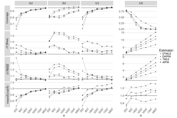
Figure 2: Results of the simulation study.

The results of the simulation are presented in Figure 2. In addition to corroborating the expected attributes of the estimators outlined in (i)-(iv) above, the following characteristics deserve further observation:

• $\hat{\theta}_{\operatorname{daipw}}$ has a much higher variance compared to all other estimators in scenario (a) for small samples ($n=200$) . This is possibly a consequence of inverse weighting by small probabilities in the definition of the correction factor $\hat{\beta}(\tilde{\eta})$ (see equation 8). This also affects $\hat{\theta}_{\operatorname{dtmle}}$, but to a lesser extent.

• $\hat{\theta}_{\operatorname{daipw}}$ and $\hat{\theta}_{\operatorname{dtmle}}$ have considerably better performance than $\hat{\theta}_{\operatorname{aipw}}$ and $\hat{\theta}_{\operatorname{tmle}}$ in scenario (b): they achieve the asymptotic efficiency bound and have significantly smaller bias.

• $\hat{\theta}_{\operatorname{daipw}}$ has smaller bias than all competitors under scenario (d).

7 Concluding Remarks

We present estimators of the effect of treatment in randomized trials with missing outcomes, where the outcomes are missing at random. One of our proposed estimators, the DTMLE, is CAN under data-adaptive estimation of the missingness probabilities and the outcome regression, under consistency of at least one of these estimators. We present the doubly-robust influence function of the estimator, which can be used to construct asymptotically valid Wald-type confidence intervals. We show that the implied asymptotic distribution is valid under a smaller set of assumptions, compared to existing estimators.

As an anonymous referee pointed out, the method of Benkeser et al. (2016) could be applied to our problem by defining $T=AM$ and estimating $E\{E(Y\mid T=1,W)\}$. We find this approach unsatisfactory because it ignores intrinsic properties of the variables $A$ and $M$, which are more appropriately exploited when modeled independently. For example, $P(A=1\mid W)$ is known in a randomized trial, and a logistic regression model with at least an intercept term provides a consistent estimator. Furthermore, covariate adjustment through such logistic model is known to improve the precision of the resulting estimator. Optimally using auxiliary information of this type involves positing separate models for the conditional distributions of $A$ and $M$.

Our proposed methods share connections with the balancing score theory for causal inference (Rubin, 1983). In particular, note that the score equations $\mathbb{P}_{n}D_{A,\tilde{g},\hat{\lambda}}=0$ and $\mathbb{P}_{n}D_{M,\tilde{g},\hat{\lambda}}=0$ are balancing equations that ensure that the empirical mean of $\hat{e}(W)$ is equal to its re-weighted mean when using weights $A_{i}/\tilde{g}_{A}(W_{i})$ and $A_{i}M_{i}/\tilde{g}(W_{i})$. Covariate balanced estimators have been traditionally used to reduce bias in observational studies and missing data models (e.g., Hainmueller, 2011; Imai and Ratkovic, 2014; Zubizarreta, 2015), but covariate selection for balancing remains an open problem. We conjecture that our theory may help to solve this problem by shedding light on key transformations of the covariates that require balance, such as $\hat{e}(W)$.

We also note that the methods presented may be readily extended to estimation of other parameters in observational data or randomized trials. In particular, the estimators for the causal effect of treatment on the quantile of an outcome presented in Díaz (2015) are amenable to the correction presented here.

Finally, Donsker Condition 2, which may be restrictive in some settings, may be removed through the use of a cross-validated version of our TMLE. Such development would follow from trivial extensions of the work of Zheng and van der Laan (2011), and would be achieved by constructing a cross-validated version of the MLE in step 2 of the TMLE algorithm presented in Section 5.

Appendix A Proofs

A.1 Theorem 1

The drift term $\beta(\hat{\eta})$ may be decomposed as

$$\beta(\hat{\eta})= \int\frac{1}{\hat{g}}\{g_{0}-\hat{g}\}\{m_{0}-m_{1}\}dP_{0}+$$ (14)

$$\int\frac{1}{g_{1}}\{g_{0}-g_{1}\}\{m_{0}-\hat{m}\}dP_{0}+$$ (15)

$$\int\frac{1}{\hat{g}}\{g_{1}-\hat{g}\}\{m_{1}-\hat{m}\}dP_{0}+$$ (16)

$$\int\left\{\frac{1}{\hat{g}}-\frac{1}{g_{1}}\right\}\{g_{0}-g_{1}\}\{m_{1}-\hat{m}\}dP_{0}+$$ (17)

$$\int\frac{1}{g_{1}}\{g_{0}-g_{1}\}\{m_{1}-m_{0}\}dP_{0}$$ (18)

Under Condition 3 we have $(\ref{t1})+(\ref{t2})=o_{P}(n^{-1/2})$, and $(\ref{t3})=0$. Denote (14) and (15) with $\beta_{g}(\hat{g})$ and $\beta_{m}(\hat{m})$, respectively. Then

$$\beta(\hat{\eta})=\beta_{g}(\hat{g})+\beta_{m}(\hat{m})+o_{P}(n^{-1/2}),$$ (19)

Define

$$\hat{\gamma}_{A,0}(W) =P_{0}\big{\{}A=1\mid m_{1}(W),\hat{m}(W)\big{\}},$$

$$\hat{\gamma}_{M,0}(W) =P_{0}\big{\{}M=1\mid A=1,m_{1}(W),\hat{m}(W)\big{\}},$$

$$\hat{r}_{A,0}(W) =E_{P_{0}}\left\{\frac{A-g_{A,1}(W)}{g_{A,1}(W)}\mathrel{\bigg{|}}m_{1}(W),\hat{m}(W)\right\},$$

$$\hat{r}_{M,0}(W) =E_{P_{0}}\left\{\frac{M-g_{M,1}(W)}{g_{1}(W)}\mathrel{\bigg{|}}A=1,m_{1}(W),\hat{m}(W)\right\},$$

$$\hat{e}_{0}(W) =E_{P_{0}}\big{\{}Y-m_{1}(W)\mid A=1,M=1,g_{1}(W),\hat{g}(W)\big{\}}.$$

First, assume $g_{1}=g_{0}$, so that $\beta(\hat{\eta})=\beta_{g}(\hat{g})+o_{P}(n^{-1/2})$. We have

$$\beta_{g}(\hat{g})= \int\frac{1}{\hat{g}(w)}\{g_{0}(w)-\hat{g}(w)\}\{m_{0}(w)-m_{1}(w)\}dP_{0}(w)$$

$$= \int\frac{a\,m}{\hat{g}(w)g_{0}(w)}\{g_{0}(w)-\hat{g}(w)\}\{y-m_{1}(w)\}dP_{0}(y,m,a,w)$$

$$= \int\left[\int\frac{a\,m}{\hat{g}(w)g_{0}(w)}\{y-m_{1}(w)\}\{g_{0}(w)-\hat{g}(w)\}dP_{0}(y\mid a,m,w,g_{0}(w),\hat{g}(w))\right]\,dP_{0}(m,a,w)$$

$$= \int\frac{a\,m\,\hat{e}_{0}(w)}{\hat{g}(w)g_{0}(w)}\{g_{0}(w)-\hat{g}(w)\}dP_{0}(m,a,w)$$

$$= \int\frac{\hat{e}_{0}(w)}{\hat{g}(w)}\{g_{0}(w)-\hat{g}(w)\}dP_{0}(w)$$

$$= \int\frac{\hat{e}_{0}(w)}{\hat{g}(w)}\{a\,m-\hat{g}(w)\}dP_{0}(m,a,w)$$

$$= \int\left[\frac{a\,\hat{e}_{0}(w)}{\hat{g}(w)}\{m-\hat{g}_{M}(w)\}+\frac{\hat{e}_{0}(w)}{\hat{g}_{A}(w)}\{a-\hat{g}_{A}(w)\}\right]dP_{0}(m,a,w)$$

$$= \int\left[\frac{a\,e_{0}(w)}{\hat{g}(w)}\{m-\hat{g}_{M}(w)\}+\frac{e_{0}(w)}{\hat{g}_{A}(w)}\{a-\hat{g}_{A}(w)\}\right]dP_{0}(m,a,w)$$ (20)

$$+\int\left[\frac{a\,\{\hat{e}_{0}(w)-e_{0}(w)\}}{\hat{g}(w)}\{m-\hat{g}_{M}(w)\}+\frac{\hat{e}_{0}(w)-e_{0}(w)}{\hat{g}_{A}(w)}\{a-\hat{g}_{A}(w)\}\right]dP_{0}(m,a,w).$$ (21)

Here $P_{0}(g_{0}(w),\hat{g}(w))$ is the distribution of the transformation $W\to(g_{0}(W),\hat{g}(W))$, where $\hat{g}$ is fixed. The third equality follows by the law of iterated expectation and is obtained by first conditioning on the joint distribution of $(M,A)$ and the transformations $g_{0}(W)$ and $\hat{g}(W)$.

The term (20) is $P_{0}\{D_{M,\hat{g},\lambda_{0}}+D_{A,\hat{g},\lambda_{0}}\}$, whereas (21) is $O_{P}\left(||\hat{g}-g_{0}||^{2}\right)$. Under Condition 3 with $g_{1}=g_{0}$ the latter term is $o_{P}(n^{-1/2})$, so that

$$\beta_{g}(\hat{g})=P_{0}\{D_{M,\hat{g},\lambda_{0}}+D_{A,\hat{g},\lambda_{0}}\}+o_{P}(n^{-1/2}).$$

The result follows because, under $g_{1}=g_{0}$ we have $e_{0}(w)=0$, and thus $D_{Y,\hat{\mu},\lambda_{0}}=0$.

Now assume $m_{1}=m_{0}$, we have $\beta(\hat{\eta})=\beta_{m}(\hat{m})+o_{P}(n^{-1/2})$. We have

$$\beta_{m}(\hat{m})= \int\frac{1}{g_{1}(w)}\{g_{0}(w)-g_{1}(w)\}\{m_{0}(w)-\hat{m}(w)\}dP_{0}(w)$$

$$= \int\left\{\frac{g_{A,0}}{g_{1}(w)}\{g_{M,0}(w)-g_{M,1}(w)\}+\frac{1}{g_{A,1}}\{g_{A,0}-g_{A,1}\}\right\}\{m_{0}(w)-\hat{m}(w)\}dP_{0}(w)$$

$$= \int\left\{\frac{a}{g_{1}(w)}\{m-g_{M,1}(w)\}+\frac{1}{g_{A,1}}\{a-g_{A,1}\}\right\}\{m_{0}(w)-\hat{m}(w)\}dP_{0}(m,a,w)$$

$$= \int\left[a\hat{r}_{M,0}(w)+\hat{r}_{A,0}(W)\right]\{m_{0}(w)-\hat{m}(w)\}dP_{0}(m,a,w)$$

$$= \int\left[\hat{\gamma}_{A}(w)\hat{r}_{M,0}(w)+\hat{r}_{A,0}(W)\right]\{m_{0}(w)-\hat{m}(w)\}dP_{0}(m,a,w)$$

$$= \int\frac{a\,m\,}{\hat{\gamma}_{A,0}(w)\hat{\gamma}_{M,0}(w)}\left[\hat{\gamma}_{A}(w)\hat{r}_{M,0}(w)+\hat{r}_{A,0}(w)\right]\{y-\hat{m}(w)\}dP_{0}(m,a,w)$$

$$= \int a\,m\left[\frac{r_{M,0}(w)}{\gamma_{M,0}(w)}+\frac{r_{A,0}(w)}{\gamma_{0}(w)}\right]\{y-\hat{m}(w)\}dP_{0}(m,a,w)+O_{P}(||\hat{m}-m_{0}||^{2})$$

Under Condition 3 with $m_{1}=m_{0}$ we have $||\tilde{m}-m_{0}||^{2}=o_{P}(n^{-1/2})$ and $r_{A,0}(w)=r_{M,0}(w)=0$. Thus $D_{M,\tilde{g},\lambda_{0}}=D_{A,\tilde{g},\lambda_{0}}=0$. This completes the proof of the theorem.

A.2 Theorem 2

Arguing as in equation (4) we get

$$\hat{\theta}_{\operatorname{dtmle}}-\theta_{0}=\beta(\tilde{\eta})+(\mathbb{P}_{n}-P_{0})D_{\eta_{1},\theta_{0}}+o_{P}\big{(}n^{-1/2}+|\beta(\tilde{\eta})|\big{)}$$

Note that, by construction (see Section 5), $\hat{\beta}(\tilde{\eta})=0$, so that Lemma 1 below gives us the asymptotic expression for $\beta(\tilde{\eta})$. Substituting this expression we get

$$\hat{\theta}_{\operatorname{tmle}}-\theta_{0}=(\mathbb{P}_{n}-P_{0})(D_{\eta_{1},\theta_{0}}-D_{M,g_{1},\lambda_{0}}-D_{A,g_{1},\lambda_{0}}-D_{Y,m_{1},\lambda_{0}})+o_{P}\big{(}n^{-1/2}+O_{P}(n^{-1/2})\big{)}.$$

The last term is $o_{P}(n^{-1/2})$. This, together with the central limit theorem concludes the proof.

Lemma 1 (Asymptotic Linearity of $\beta(\hat{\eta})$).

Assume Condition 2 and Condition 3. Then

$$\beta(\hat{\eta})-\hat{\beta}(\hat{\eta})=-(\mathbb{P}_{n}-P_{0})\{D_{M,g_{1},\lambda_{0}}+D_{A,g_{1},\lambda_{0}}+D_{Y,m_{1},\lambda_{0}}\}+o_{P}(n^{-1/2}).$$

Proof From Theorem 1, we have

$$\beta(\hat{\eta})=P_{0}\{D_{A,\hat{g},\lambda_{0}}+D_{M,\hat{m},\lambda_{0}}+D_{Y,\hat{m},\lambda_{0}}\}+o_{P}(n^{-1/2})$$

Next, we show that $P_{0}D_{Y,\hat{m},\lambda_{0}}-\mathbb{P}_{n}D_{Y,\hat{m},\hat{\lambda}}=-(\mathbb{P}_{n}-P_{0})D_{Y,m_{1},\lambda_{0}}+o_{P}(n^{-1/2}).$ The result for the other terms follow an analogous analysis.

If $g_{1}(w)=g_{0}(w)$ we have $r_{A,0}(w)=r_{M,0}(w)=0$, which implies $D_{Y,\hat{m},\lambda_{0}}(o)=D_{Y,m_{1},\lambda_{0}}(o)=0$, and the result follows trivially. If $m_{1}=m_{0}$, we have

$$P_{0}D_{Y,\hat{m},\lambda_{0}}-\mathbb{P}_{n}D_{Y,\hat{m},\hat{\lambda}}=-(\mathbb{P}_{n}-P_{0})D_{Y,\hat{m},\hat{\lambda}}+P_{0}(D_{Y,\hat{m},\lambda_{0}}-D_{Y,\hat{m},\hat{\lambda}}),$$

where we added and subtracted $P_{0}D_{Y,\hat{m},\hat{\lambda}}$. We have

$$P_{0}(D_{Y,\hat{m},\lambda_{0}}-D_{Y,\hat{m},\hat{\lambda}})=\int g_{0}\left\{\frac{r_{M,0}}{\gamma_{M,0}}-\frac{\hat{r}_{M}}{\hat{\gamma}_{M}}+\frac{r_{A,0}}{\gamma_{0}}-\frac{\hat{r}_{A}}{\hat{\gamma}}\right\}\{m_{0}-\hat{m}\}dP_{0}$$

Using the Cauchy-Schwartz and triangle inequalities, we obtain

$$P_{0}(D_{Y,\hat{m},\lambda_{0}}-D_{Y,\hat{m},\hat{\lambda}})=O_{P}\big{(}||\hat{m}-m_{0}||\{||\hat{r}_{A}-r_{A,0}||+||\hat{r}_{M}-r_{M,0}||+||\hat{\gamma}_{A}-\gamma_{A,0}||+||\hat{\gamma}_{M}-\gamma_{M,0}||\}\big{)}$$

In light of Lemma 2 below we get

$$P_{0}(D_{Y,\hat{m},r_{0}}-D_{Y,\hat{m},\hat{r}})=O_{P}\big{(}||\hat{m}-m_{0}||\{||\hat{g}-g_{1}||+||\hat{m}-m_{0}||+n^{-7/20}\}\big{)}.$$

By Condition 3 this term is $o_{P}(n^{-1/2})$.

Under Condition 2 and Condition 3, $D_{Y,\hat{m},\hat{\lambda}}$ an application of Theorem 4 of Giné and Nickl (2008) and example 2.10.10 of van der Vaart and Wellner (1996) yields that $D_{Y,\hat{m},\hat{\lambda}}$ is in a Donsker class. Thus, according to theorem 19.24 of van der Vaart (1998): $P_{0}D_{Y,\hat{\eta},\lambda_{0}}-\mathbb{P}_{n}D_{Y,\hat{m},\hat{\lambda}}=-(\mathbb{P}_{n}-P_{0})D_{Y,\eta_{1},\gamma_{0}}+o_{P}(n^{-1/2})$. ∎

Lemma 2.

Assume $\hat{\gamma}_{A}$, $\hat{\gamma}_{M}$, and $\hat{\mu}$ use the bandwidth $\hat{h}=n^{-0.1}\hat{h}_{\operatorname{opt}}$ and $K_{h}$ is a second order kernel. Then

$$||\hat{\gamma}_{A}-\gamma_{A,0}|| =O_{P}\big{(}||\hat{g}-g_{1}||+||\hat{m}-m_{1}||+n^{-7/20}\big{)}$$

$$||\hat{\gamma}_{M}-\gamma_{M,0}|| =O_{P}\big{(}||\hat{g}-g_{1}||+||\hat{m}-m_{1}||+n^{-7/20}\big{)}$$

$$||\hat{r}_{A}-r_{A,0}|| =O_{P}\big{(}||\hat{g}-g_{1}||+||\hat{m}-m_{1}||+n^{-7/20}\big{)}$$

$$||\hat{r}_{M}-r_{M,0}|| =O_{P}\big{(}||\hat{g}-g_{1}||+||\hat{m}-m_{1}||+n^{-7/20}\big{)}$$

$$||\hat{e}-e_{0}|| =O_{P}\big{(}||\hat{g}-g_{1}||+||\hat{m}-m_{1}||+n^{-7/20}\big{)}$$

Proof We prove the result for $\hat{e}$. The proofs for the other components of $\hat{\lambda}$ follow symmetric arguments. Let

$$\hat{e}_{0}(w)=\frac{\sum_{i=1}^{n}A_{i}M_{i}K_{\hat{h}}\{g_{1}(W_{i})-g_{1}(w)\}\{Y_{i}-m_{1}(W_{i})\}}{\sum_{i=1}^{n}A_{i}M_{i}K_{\hat{h}}\{g_{1}(W_{i})-g_{1}(w)\}}$$

denote the kernel regression estimator that would be computed if $m_{1}$ and $g_{1}$ were known. The triangle inequality yields

$$||\hat{e}-e_{0}||\leq||\hat{e}-\hat{e}_{0}||+||\hat{e}_{0}-e_{0}||$$

Under the conditions of the lemma, since $\hat{h}=n^{-0.1}\hat{h}_{\operatorname{opt}}$ is an undersmoothing bandwidth, the leading term of $||\hat{e}_{0}-e_{0}||^{2}$ is the variance of a kernel estimator, which is of order $n^{-1}\hat{h}^{-1}=O_{P}(n^{-7/10})$, which yields $||\hat{e}_{0}-e_{0}||=O_{P}(n^{-7/20})$. The first term concerns estimation of $\mu_{1}$ and $g_{1}$ and may be analyzed as follows. To simplify notation, for a given $g$, let

$$K^{\star}_{g,i}(x)=\frac{K_{\hat{h}}\{g(X_{i})-g(x)\}}{\sum_{i=1}^{n}K_{\hat{h}}\{g(X_{i})-g(x)\}}.$$

Thus

$$\hat{e}(x)-\hat{e}_{0}(x)= \sum_{i=1}^{n}A_{i}M_{i}K^{\star}_{\hat{g},i}(x)\{Y_{i}-\hat{m}(X_{i})\}-\sum_{i=1}^{n}A_{i}M_{i}K^{\star}_{g_{1},i}(x)\{Y_{i}-m_{1}(X_{i})\}$$

$$= \sum_{i=1}^{n}A_{i}M_{i}\{K^{\star}_{\hat{g},i}(x)-K^{\star}_{g_{1},i}(x)\}\{Y_{i}-\hat{m}(X_{i})\}$$

$$+\sum_{i=1}^{n}A_{i}M_{i}K^{\star}_{g_{1},i}(x)\{m_{1}(X_{i})-\hat{m}(X_{i})\}.$$

Taking $||\cdot||$ on both sides along with the triangle inequality yields the result in the lemma. ∎

Appendix B R code

References

- Bang and Robins (2005) Heejung Bang and James M Robins. Doubly robust estimation in missing data and causal inference models. Biometrics, 61(4):962–973, 2005.
- Bembom et al. (2008) O. Bembom, J.W. Fessel, R.W. Shafer, and M.J. van der Laan. Data-adaptive selection of the adjustment set in variable importance estimation. 2008. URL http://www.bepress.com/ucbbiostat/paper231.
- Benkeser et al. (2016) David Benkeser, Marco Carone, Mark J van der Laan, and Peter Gilbert. Doubly-robust nonparametric inference on the average treatment effect. Technical Report 356, U.C. Berkeley Division of Biostatistics Working Paper Series, 2016.
- Bolthausen et al. (2002) Erwin Bolthausen, Edwin Perkins, and van der Vaart Aad. Lectures on Probability Theory and Statistics: Ecole D’Eté de Probabilités de Saint-Flour XXIX-1999. Springer Science & Business Media, 2002.
- Colantuoni and Rosenblum (2015) Elizabeth Colantuoni and Michael Rosenblum. Leveraging prognostic baseline variables to gain precision in randomized trials. Statistics in Medicine, 34(18):2602–2617, 2015. ISSN 1097-0258. doi: 10.1002/sim.6507. URL http://dx.doi.org/10.1002/sim.6507.
- Díaz (2015) Iván Díaz. Efficient estimation of quantiles in missing data models. arXiv preprint arXiv:1512.08110, 2015.
- Díaz et al. (2016) Iván Díaz, Elizabeth Colantuoni, and Michael Rosenblum. Enhanced precision in the analysis of randomized trials with ordinal outcomes. Biometrics, 72(2):422–431, 2016. ISSN 1541-0420. doi: 10.1111/biom.12450. URL http://dx.doi.org/10.1111/biom.12450.
- Giné and Nickl (2008) Evarist Giné and Richard Nickl. Uniform central limit theorems for kernel density estimators. Probability Theory and Related Fields, 141(3-4):333–387, 2008.
- Gruber and van der Laan (2010) Susan Gruber and Mark J van der Laan. A targeted maximum likelihood estimator of a causal effect on a bounded continuous outcome. The International Journal of Biostatistics, 6(1), 2010.
- Hahn (1998) Jinyong Hahn. On the role of the propensity score in efficient semiparametric estimation of average treatment effects. Econometrica, pages 315–331, 1998.
- Hainmueller (2011) Jens Hainmueller. Entropy balancing for causal effects: A multivariate reweighting method to produce balanced samples in observational studies. Political Analysis, page mpr025, 2011.
- Hammer et al. (1996) Scott M Hammer, David A Katzenstein, Michael D Hughes, Holly Gundacker, Robert T Schooley, Richard H Haubrich, W Keith Henry, Michael M Lederman, John P Phair, Manette Niu, et al. A trial comparing nucleoside monotherapy with combination therapy in hiv-infected adults with cd4 cell counts from 200 to 500 per cubic millimeter. New England Journal of Medicine, 335(15):1081–1090, 1996.
- Imai and Ratkovic (2014) Kosuke Imai and Marc Ratkovic. Covariate balancing propensity score. Journal of the Royal Statistical Society: Series B (Statistical Methodology), 76(1):243–263, 2014.
- Juraska et al. (2012) Michal Juraska, with contributions from Peter B. Gilbert, Xiaomin Lu, Min Zhang, Marie Davidian, and Anastasios A. Tsiatis. speff2trial: Semiparametric efficient estimation for a two-sample treatment effect, 2012. URL https://CRAN.R-project.org/package=speff2trial. R package version 1.0.4.
- Kang and Schafer (2007) J. Kang and J. Schafer. Demystifying double robustness: A comparison of alternative strategies for estimating a population mean from incomplete data (with discussion). Statistical Science, 22:523–39, 2007.
- Koch et al. (1998) Gary G Koch, Catherine M Tangen, Jin-Whan Jung, and Ingrid A Amara. Issues for covariance analysis of dichotomous and ordered categorical data from randomized clinical trials and non-parametric strategies for addressing them. Statistics in medicine, 17(15-16):1863–1892, 1998.
- Lee et al. (2010) Brian K Lee, Justin Lessler, and Elizabeth A Stuart. Improving propensity score weighting using machine learning. Statistics in medicine, 29(3):337–346, 2010.
- Moore and van der Laan (2009) Kelly L Moore and Mark J van der Laan. Covariate adjustment in randomized trials with binary outcomes: Targeted maximum likelihood estimation. Statistics in Medicine, 28(1):39–64, 2009.
- Neugebauer et al. (2016) Romain Neugebauer, Julie A Schmittdiel, and Mark J van der Laan. A case study of the impact of data-adaptive versus model-based estimation of the propensity scores on causal inferences from three inverse probability weighting estimators. The international journal of biostatistics, 12(1):131–155, 2016.
- Polley et al. (2016) Eric Polley, Erin LeDell, and Mark van der Laan. SuperLearner: Super Learner Prediction, 2016. URL https://CRAN.R-project.org/package=SuperLearner. R package version 2.0-19.
- Porter et al. (2011) Kristin E. Porter, Susan Gruber, Mark J. van der Laan, and Jasjeet S. Sekhon. The relative performance of targeted maximum likelihood estimators. The International Journal of Biostatistics, 7(1):1–34, 2011.
- Ridgeway and McCaffrey (2007) Greg Ridgeway and Daniel F. McCaffrey. Comment: Demystifying double robustness: A comparison of alternative strategies for estimating a population mean from incomplete data. Statist. Sci., 22(4):540–543, 11 2007. doi: 10.1214/07-STS227C. URL http://dx.doi.org/10.1214/07-STS227C.
- Robins et al. (2007) James Robins, Mariela Sued, Quanhong Lei-Gomez, and Andrea Rotnitzky. Comment: Performance of double-robust estimators when” inverse probability” weights are highly variable. Statistical Science, 22(4):544–559, 2007.
- Robins et al. (1994) J.M. Robins, A. Rotnitzky, and L.P. Zhao. Estimation of regression coefficients when some regressors are not always observed. Journal of the American Statistical Association, 89(427):846–866, September 1994.
- Rubin (1987) Donald B Rubin. Multiple Imputation for Nonresponse in Surveys. John Wiley & Sons, 1987.
- Rubin (1983) P.R. Rosenbaum & D.B. Rubin. The central role of the propensity score in observational studies for causal effects. Biometrika, 70:41–55, 1983.
- Tan (2010) Zhiqiang Tan. Bounded, efficient and doubly robust estimation with inverse weighting. Biometrika, 97(3):661–682, 2010.
- van der Laan (2014) Mark J van der Laan. Targeted estimation of nuisance parameters to obtain valid statistical inference. The international journal of biostatistics, 10(1):29–57, 2014.
- van der Laan (2015) Mark J van der Laan. A generally efficient targeted minimum loss based estimator. Technical Report 343, U.C. Berkeley Division of Biostatistics Working Paper Series, 2015.
- van der Laan and Starmans (2014) Mark J van der Laan and Richard JCM Starmans. Entering the era of data science: Targeted learning and the integration of statistics and computational data analysis. Advances in Statistics, 2014, 2014.
- van der Laan and Robins (2003) M.J. van der Laan and J.M. Robins. Unified Methods for Censored Longitudinal Data and Causality. Springer, New York, 2003.
- van der Laan and Rose (2011) M.J. van der Laan and S. Rose. Targeted Learning: Causal Inference for Observational and Experimental Data. Springer, New York, 2011.
- van der Laan and Rubin (2006) M.J. van der Laan and D. Rubin. Targeted maximum likelihood learning. The International Journal of Biostatistics, 2(1):Article 11, 2006.
- van der Laan et al. (2005) M.J. van der Laan, M.L. Petersen, and M.M. Joffe. History-adjusted marginal structural models & statically-optimal dynamic treatment regimens. The International Journal of Biostatistics, 1(1):10–20, 2005.
- van der Laan et al. (2007) M.J. van der Laan, E. Polley, and A. Hubbard. Super learner. Statistical Applications in Genetics & Molecular Biology, 6(25):Article 25, 2007.
- van der Laan (2006) Y. Wang & O. Bembom & M.J. van der Laan. Data adaptive estimation of the treatment specific mean. Journal of Statistical Planning & Inference, 2006.
- van der Vaart (1998) A. W. van der Vaart. Asymptotic Statistics. Cambridge University Press, 1998.
- van der Vaart and Wellner (1996) A. W. van der Vaart and J. A. Wellner. Weak Convergence and Emprical Processes. Springer-Verlag New York, 1996.
- van der Vaart et al. (2006) A.W. van der Vaart, S. Dudoit, and M.J. van der Laan. Oracle inequalities for multi-fold cross-validation. Statistics & Decisions, 24(3):351–371, 2006.
- Vermeulen and Vansteelandt (2015) Karel Vermeulen and Stijn Vansteelandt. Bias-reduced doubly robust estimation. Journal of the American Statistical Association, 110(511):1024–1036, 2015.
- Vermeulen and Vansteelandt (2016) Karel Vermeulen and Stijn Vansteelandt. Data-adaptive bias-reduced doubly robust estimation. The international journal of biostatistics, 12(1):253–282, 2016.
- Zhang et al. (2008) Min Zhang, Anastasios A Tsiatis, and Marie Davidian. Improving efficiency of inferences in randomized clinical trials using auxiliary covariates. Biometrics, 64(3):707–715, 2008.
- Zheng and van der Laan (2011) Wenjing Zheng and Mark J van der Laan. Cross-validated targeted minimum-loss-based estimation. In Targeted Learning, pages 459–474. Springer, 2011.
- Zubizarreta (2015) José R Zubizarreta. Stable weights that balance covariates for estimation with incomplete outcome data. Journal of the American Statistical Association, 110(511):910–922, 2015.