Approximating Lyapunov Exponents and Stationary Measures

Abstract.

We give a new proof of E. Le Page’s theorem on the Hölder continuity of the first Lyapunov exponent in the class of irreducible Bernoulli cocycles. This suggests an algorithm to approximate the first Lyapunov exponent, as well as the stationary measure, for such random cocycles.

Keywords: Lyapunov exponent, random cocycle, stationary measure.

AMS subject classification: 37H15, 37D25.

1. Introduction

The description of the behavior of random linear cocycles is a classical subject studied in different mathematical fields: it can be seen as a non-commutative random walk in Probability Theory, it relates to discrete Schrödinger operators describing a particle under a random potential in Quantum Mechanics, and it can also be regarded as toy model for the differential’s dynamics of an ergodic diffeomorphism over a compact manifold in Dynamical Systems. An important feature in all these settings are the Lyapunov exponents (LE), describing the exponential growth of norms of vectors under the action of the linear cocycle.

In Probability Theory the top Lyapunov exponent of a random Bernoulli cocycle measures the asymptotic behaviour $L_{1}:=\lim_{n\to+\infty}\frac{1}{n}\log\left\|M_{n}\right\|$ of the matrix products $M_{n}=X_{n-1}\,\cdots\,X_{1}\,X_{0}$ of i.i.d. processes $\{X_{n}\}_{\geq 0}$ with values in some matrix group like ${\rm GL}_{d}(\mathbb{R})$. In this context, H. Furstenberg [4] gave an explicit integral formula for the largest Lyapunov exponent in terms of a stationary measure for the action of the i.i.d. process $\{X_{n}\}$ on the projective space $\mathbb{P}(\mathbb{R}^{d})$. He also gave simple sufficient conditions for the top Lyapunov exponent to be non zero.

Such random linear cocycles can be described by the choice of a compact metric space $\Sigma$, a Borel probability measure $\mu$ on $\Sigma$ and a measurable function $A\colon\Sigma\to{\rm GL}_{d}(\mathbb{R})$. If $\{Z_{n}\}_{n\geq 0}$ is a $\Sigma$-valued i.i.d. process with common distribution $\mu$, then $X_{n}=A(Z_{n})$ is an i.i.d. ${\rm GL}_{d}(\mathbb{R})$-valued process which determines a random Bernoulli cocycle.

A natural question that arises is the continuity of the dependence of the top Lyapunov exponent $L_{1}$ as a function of $A$ and $\mu$. A related important question is how to get good estimates for the top Lyapunov exponent of a given cocycle. Because Furstenberg’s formula depends on a stationary measure which typically is not known in any explicit way, this problem has no obvious solution. The issue here is precisely to estimate the stationary measure. Similar results were obtained recently by S. Galatolo et. al. (see [6, 7]), regarding the problem of approximating invariant measures, but working directly with transfer operators acting on measures and densities.

Fixing the measure $\mu$ and assuming that the matrices $A$ preserve some cone family (which means that the cocycle is uniformly hyperbolic) Ruelle [14] was able to show that the top Lyapunov exponent depends analytically on $A$. In this setting M. Pollicott [12] obtained also a very efficient method to approximate the exponent numerically.

On the other hand, dropping the uniform hyperbolicity assumption makes the continuity issue much more subtle and less regular. E. Le Page [10] was able to show, under some general irreducibility assumption, a Hölder continuous dependence of the top Lyapunov exponent as a function of $A$. In this same setting, an example due to B. Halperin (see Simon-Taylor [15]) shows that the Hölder modulus of continuity can not be improved.

Now if $\Sigma=\{1,\ldots,k\}$ is finite then the function $A$ takes a finite number of values $A_{1},\ldots,A_{k}$. Considering a probability measure $\mu=p_{1}\delta_{1}+\cdots+p_{k}\delta_{k}$ on $\Sigma$ with $p_{i}>0$ for all $i=1,\ldots,k$ and $\sum_{j=1}^{k}p_{j}=1$, Y. Peres [11] was able to prove the analiticity of the top Lypaunov exponent continuity with respect to the measure $\mu$.

In this text we revisit these continuity results dealing with the dependence on $A$ and on $\mu$ in a unified way, re-obtaining Le Page’s result with a simpler proof and partially improving on Peres’ result (see Theorem 1 and Remark 2). We work with the adjoint of the usual transfer operator acting on probability measures. Under a suitable irreducibility assumption, this adjoint operator, still referred as a transfer operator, acts on spaces of Hölder continuous observables with nice contracting properties: it is a quasi-compact operator with simple maximal eigenvalue [1, 10]. The technique gives a method to approximate the stationary measure in Furstenberg formula when the original transfer operator is replaced by a finite-dimensional approximation (see Theorem 4), what also provides a way to estimate the top Lyapunov exponent. At the end we illustrate the method with a couple of examples.

The paper is organized as follows: In Section 2 we introduce the main concepts, definitions, and we state our result on the continuity of the top Lyapunov exponent (Theorem 1). In Section 3 we define the main tool to deal with stationary measures, the so called transfer operators. Here we prove an abstract continuity theorem for transfer operators (see Theorem 3). In sections 4 and 5 we prove Theorem 1. In Section 6 we state and prove an approximation theorem (Theorem 4). We also describe a method to estimate the stationary measure and the top Lyapunov exponent of a random cocycle. In Section 7 we illustrate the approximation method with a couple of examples. Section 8 is an appendix where we establish some geometric inequalities.

2. Random linear cocycles

A measure preserving transformation is a tuple $(T,\Omega,\mathscr{F},\mathbb{P})$ where $T\colon\Omega\to\Omega$ is a bi-measurable automorphism of the measurable space $(\Omega,\mathscr{F})$, and $(\Omega,\mathscr{F},\mathbb{P})$ is a probability space such that $\mathbb{P}(T^{-1}E)=\mathbb{P}(E)$ for all $E\in\mathscr{F}$. Such a transformation $(T,\Omega,\mathscr{F},\mathbb{P})$ is said to be ergodic when $\mathbb{P}(E)=0$ or $\mathbb{P}(E)=1$ for every $E\in\mathscr{F}$ such that $T^{-1}E=E$.

We call linear cocycle over $(T,\Omega,\mathscr{F},\mathbb{P})$ to a map $F_{A}\colon\Omega\times\mathbb{R}^{d}\to\Omega\times\mathbb{R}^{d}$ of the form $F_{A}(\omega,v):=(T\omega,A(x)\,v)$, determined by a measurable function $A\colon\Omega\to{\rm GL}_{d}(\mathbb{R})$. Since $F_{A}$ is determined by $A$, we will refer to $A$ as the linear cocycle. The cocycle $A$ is called integrable when

$$\mathbb{E}(\log_{+}\left\|A^{\pm 1}\right\|):=\int_{\Omega}\log_{+}\left\|A^{\pm 1}\right\|\,\mathrm{d}\mathbb{P}<+\infty.$$

The iterates $F_{A}^{n}$ of the cocycle $A$ are given by $F_{A}^{n}(\omega,v)=(T^{n},A^{n}(\omega)v)$ where

$$A^{n}(\omega):=\left\{\begin{array}[]{lll}A(T^{n-1}\omega)\cdots A(T\omega)\,A(\omega)&\text{ if }&n\geq 0\\ A(T^{-n}\omega)^{-1}\cdots A(T^{-2}\omega)^{-1}\,A(T^{-1}\omega)^{-1}&\text{ if }&n<0\end{array}\right.$$

The top Lyapunov exponent of a linear cocycle $A$ is the first of the following two limits established by H. Furstenberg and H. Kesten [3]:

Theorem (Furstenberg-Kesten).

Let $(T,\Omega,\mathscr{F},\mathbb{P})$ be an ergodic transformation, and $A\colon\Omega\to{\rm GL}_{d}(\mathbb{R})$ an integrable measurable random variable. Then the the following limits exist $\mathbb{P}$-almost surely,

$$\gamma_{+}(A) =\lim_{n\to\pm\infty}\frac{1}{n}\,\log\left\|A^{n}(\omega)\right\|,$$

$$\gamma_{-}(A) =\lim_{n\to\pm\infty}\frac{1}{n}\,\log\left\|A^{n}(\omega)^{-1}\right\|^{-1}.$$

Given a matrix $M\in{\rm M}_{d}(\mathbb{R})$ its singular values are the square roots of the eigenvalues of the positive semi-definite symmetric matrix $M^{T}M$. The sorted singular values of $M$ are denoted by

$$s_{1}(M)\geq s_{2}(M)\geq\cdots\geq s_{d}(M)\geq 0.$$

The first singular value is the matrix’s norm, $s_{1}(M)=\left\|M\right\|$, which reflects the maximum expansion factor of $M$’s action on the Euclidean space $\mathbb{R}^{d}$. Likewise, the last singular value $s_{d}(M)$ is the minimum expansion factor of $M$. One has $s_{d}(M)=0$ if $M$ is non-invertible, and $s_{d}(M)=\left\|M^{-1}\right\|^{-1}$ otherwise.

Given $k\in\mathbb{N}$, we denote by $\wedge_{k}M$ the $k$-th exterior power of $M$. This is a matrix which represents the action of $M$ on the space $\wedge_{k}\mathbb{R}^{d}$ of $k$-th exterior vectors of $\mathbb{R}^{d}$ (see [16]), and whose norm can be expressed in terms of singular values

$$\left\|\wedge_{k}M\right\|=s_{1}(M)\,s_{2}(M)\,\cdots\,s_{k}(M).$$

It follows that for all $i=1,\ldots,d$,

$$s_{i}(M)=\frac{\left\|\wedge_{i}M\right\|}{\left\|\wedge_{i-1}M\right\|}.$$

Let now $A\colon\Omega\to{\rm GL}_{d}(\mathbb{R})$ be an integrable cocycle over some ergodic transformation $(T,\Omega,\mathcal{F},\mathbb{P})$. The ordered Lyapunov exponents of $A$ are defined to be the $\mathbb{P}$-almost sure limits

$$L_{i}(A)=\lim_{n\to+\infty}\frac{1}{n}\,\log s_{i}(A^{n})=\lim_{n\to+\infty}\frac{1}{n}\,\left(\log\left\|\wedge_{i}A^{n}\right\|-\log\left\|\wedge_{i}A^{n}\right\|\right),$$

where the right-hand-side limit exists by Furstenberg-Kesten’s theorem applied to the integrable exterior power cocycles $\wedge_{i}A$. One has of course

$$\gamma_{+}(A)=L_{1}(A)\;\text{ and }\;\gamma_{-}(A)=L_{d}(A).$$

From now on we will use only the notation $L_{1}(A)$ for the top Lyapunov exponent.

Given a compact metric space $(\Sigma,d)$ (the symbol space) consider the space of sequences $\Omega_{\Sigma}=\Sigma^{\mathbb{Z}}$ endowed with the product topology. The homeomorphism $T\colon\Omega_{\Sigma}\to\Omega_{\Sigma}$, $T\{\omega_{i}\}_{i\in\mathbb{Z}}:=\{\omega_{i+1}\}_{i\in\mathbb{Z}}$, is called the full shift map.

Denote by $\mbox{Prob}(\Sigma)$ the space of Borel probability measures on $\Sigma$. For a given measure $\mu\in\mbox{Prob}(\Sigma)$ consider the product probability measure $\mathbb{P}_{\mu}=\mu^{\mathbb{Z}}$ on $\Omega_{\Sigma}$. Then $(T,\Omega_{\Sigma},\mathscr{B},\mathbb{P}_{\mu})$ is an ergodic transformation, referred as a full Bernoulli shift.

A probability $\mu\in\mbox{Prob}(\Sigma)$ and a continuous function $A\colon\Sigma\to{\rm GL}_{d}(\mathbb{R})$ determine a measurable function $\tilde{A}\colon\Omega_{\Sigma}\to{\rm GL}_{d}(\mathbb{R})$, $\tilde{A}\{\omega_{n}\}_{n\in\mathbb{Z}}=A(\omega_{0})$, and hence a linear cocycle $F_{(A,\mu)}\colon\Omega_{\Sigma}\times\mathbb{R}^{d}\to\Omega_{\Sigma}\times\mathbb{R}^{d}$ over the Bernoulli shift $(T,\Omega_{\Sigma},\mathscr{B}_{\Sigma},\mathbb{P}_{\mu})$. We refer to the cocycle $F_{(A,\mu)}$ as a random cocycle. The pair $(A,\mu)\in\mathscr{C}(\Sigma,{\rm GL}_{d}(\mathbb{R}))\times\mbox{Prob}(\Sigma)$ is also referred as a random cocycle. The $n$-th iterate $F_{(A,\mu)}^{n}=F_{(A^{n},\mu^{n})}$ is the random cocycle determined by the pair $(A^{n},\mu^{n})$ where $\mu^{n}:=\mu\times\cdots\times\mu\in\mbox{Prob}(\Sigma^{n})$ and $A^{n}\colon\Sigma^{n}\to{\rm GL}_{d}(\mathbb{R})$ is the function

$$A^{n}(x_{0},x_{1},\ldots,x_{n-1}):=A(x_{n-1})\cdots A(x_{1})\,A(x_{0}).$$

The top Lyapunov exponent of the random cocycle $(A,\mu)$ will be denoted by $L_{1}(A,\mu)$.

Given a matrix $A\in{\rm GL}_{d}(\mathbb{R})$ we denote by $\Phi_{A}\colon\mathbb{P}(\mathbb{R}^{d})\to\mathbb{P}(\mathbb{R}^{d})$ its projective action.

Definition 1.

A measure $\nu\in\mbox{Prob}(\mathbb{P}(\mathbb{R}^{d}))$ is called stationary w.r.t. $(A,\mu)$ when

$$\nu=\int_{\Sigma}(\Phi_{A(x)})_{\ast}\nu\,d\mu(x).$$

Proposition 1 (Furstenberg’s formula [5]).

For any random cocycle $(A,\mu)$ there exist stationary measures $\nu\in\mbox{Prob}(\mathbb{P}(\mathbb{R}^{d}))$ such that

$$L_{1}(A,\mu)=\int_{\Sigma}\int_{\mathbb{P}(\mathbb{R}^{d})}\log\left\|A(x)\,p\right\|\,d\nu(\hat{p})\,d\mu(x).$$ (1)

Definition 2 (see Définition 2.7 in [1]).

A cocycle $(A,\mu)$ is called quasi-irreducible if there is no proper subspace $V\subset\mathbb{R}^{d}$ which is invariant under all matrices of the cocycle, i.e., such that $A(x)V=V$ for $\mu$-a.e. $x\in\Sigma$, and where $L_{1}(A|_{V})\leq L_{2}(A)$.

Remark 1.

If a cocycle $(A,\mu)$ is quasi-irreducible then it admits a unique stationary measure $\nu\in\mbox{Prob}(\mathbb{P}(\mathbb{R}^{d}))$. Thus, in this case $L_{1}(A,\mu)$ is uniquely determined by the probability $\nu$ through Furstenberg’s formula (1).

The space of cocycles $\mathscr{C}(\Sigma,{\rm GL}_{d}(\mathbb{R}))$ is endowed with the distance

$$d_{\infty}(A,B)=\max_{x\in\Sigma}\left\|A(x)-B(x)\right\|.$$

On the space $\mbox{Prob}(\Sigma)$ we consider the total variation metric, which is defined by

$$d(\mu_{1},\mu_{2}):=\left\|\mu_{1}-\mu_{2}\right\|$$

where $\left\|\mu\right\|$ stands for the total variation of a measure $\mu$.

Definition 3.

We define the space $\mathfrak{C}_{d}(\Sigma)$ of all cocycles $(A,\mu)\in\mathscr{C}(\Sigma,{\rm GL}_{d}(\mathbb{R}))\times\mbox{Prob}(\Sigma)$ such that

1. $(A,\mu)$ is quasi-irreducible and

2. $L_{1}(A,\mu)>L_{2}(A,\mu)$.

Theorem 1.

The function $L_{1}\colon\mathfrak{C}_{d}(\Sigma)\to\mathbb{R}$ is

1. locally Hölder continuous w.r.t. the metrics $d_{\infty}$ and $d$,

2. is locally Lipschitz continuous in the variable $\mu$ w.r.t. $d$.

Proof.

Follows from Propositions 4 and 5. ∎

Remark 2.

The Hölder continuous dependence of $L_{1}(A,\mu)$ on $A$ is basically E. Le Page’s [10, Théorème 1]. Item (2) improves Y. Peres’s [11, Theorem 1] in the sense that measure here may have infinite support. Our result is of course weaker in the sense that we only prove Lipschitz continuity while Y. Peres proves analiticity of the LE.

A coarser metric (and topology) can be introduced with respect to which the top LE is still Hölder continuous. Let ${\rm Diff}^{0}(\Sigma)$ denote the $\infty$-dimensional group of homeomorphisms $h\colon\Sigma\to\Sigma$. Given $\mu\in\mbox{Prob}(\Sigma)$ its $h$-pullback is the probability measure $h^{\ast}\mu:=(h^{-1})_{\ast}\mu=\mu\circ h^{-1}$. Analogously, given a cocycle $(A,\mu)$ we define its $h$-pullback as $(A\circ h,h^{\ast}\mu)$. The cocycles $F_{(A,\mu)}$ and $F_{(A\circ h,h^{\ast}\mu)}$ are conjugated via the isomorphism $H\colon\Omega_{\Sigma}\times\mathbb{R}^{d}\to\Omega_{\Sigma}\times\mathbb{R}^{d}$, $H(\{\omega_{n}\}_{n\in\mathbb{Z}},v):=(\{h(\omega_{n})\}_{n\in\mathbb{Z}},v)$. In particular we have

$$L_{1}(A,\mu)=L_{1}(A\circ h,h^{\ast}\mu).$$

Thus if one defines the metric

$$\rho((A,\mu),(B,\nu)):=\inf\left\{\,d_{\infty}(B,A\circ h)+d(\nu,h^{\ast}\mu)\,\colon\,h\in{\rm Diff}^{0}(\Sigma)\,\right\}$$

the function $L_{1}\colon\mathfrak{C}_{d}(\Sigma)\to\mathbb{R}$ is still locally Hölder w.r.t. $\rho$.

3. Transfer Operators

Let $X$ be a compact metric space. Given $0\leq\alpha\leq 1$, we denote by $\mathscr{H}_{\alpha}(X)$ the space of $\alpha$-Hölder continuous functions on $X$. On this space consider the seminorm $v_{\alpha}\colon\mathscr{H}_{\alpha}(X)\to\mathbb{R}$ defined by

$$v_{\alpha}(\varphi):=\mathrm{diam}(X)^{\alpha}\,\sup_{\begin{subarray}{c}x\neq y\\ x,y\in X\end{subarray}}\frac{|{\varphi(x)-\varphi(y)}|}{d(x,y)^{\alpha}}.$$

The space $\mathscr{H}_{\alpha}(X)$ is a Banach space (in fact a a Banach algebra with unity [2, Proposition 5.4]) when endowed with the norm

$$\left\|\varphi\right\|_{\alpha}:=v_{\alpha}(\varphi)+\left\|\varphi\right\|_{\infty}.$$

The family of semi-normed spaces $\{(\mathscr{H}_{\alpha}(X),v_{\alpha})\}_{\alpha\in[0,1]}$ is a scale in sense that for all $0\leq\alpha<\beta\leq 1$, $0\leq t\leq 1$ and $\varphi\in\mathscr{H}_{\alpha}(X)$,

1. $\mathscr{H}_{\alpha}(X)\subset\mathscr{H}_{\beta}(X)$,

2. $v_{\alpha}(\varphi)\leq v_{\beta}(\varphi)$,

3. $v_{(1-t)\alpha+t\beta}(\varphi)\leq v_{\alpha}(\varphi)^{1-t}v_{\beta}(\varphi)^{t}$.

Remark that $\mathscr{H}_{0}(X)$ coincides with the space $\mathscr{C}(X)$ of continuous functions on $X$. Moreover, for any $\varphi\in\mathscr{C}(X)$ and $x_{0}\in X$,

$$\left\|\varphi-\varphi(x_{0})\right\|_{\infty}\leq v_{0}(\varphi)\leq\left\|\varphi\right\|_{\infty}.$$

We denote by ${\bf 1}$ the constant function $1$.

Definition 4.

A linear operator $\mathscr{L}\colon\mathscr{C}(X)\to\mathscr{C}(X)$ is called a Markov operator when for all $\varphi\in\mathscr{C}(X)$,

1. $\mathscr{L}{\bf 1}={\bf 1}$,

2. $\varphi\geq 0$ implies $\mathscr{L}\varphi\geq 0$,

3. $\left\|\mathscr{L}\varphi\right\|_{\infty}\leq\left\|\varphi\right\|_{\infty}$.

Definition 5.

Given $0<\sigma<1$ and $0<\alpha\leq 1$, a Markov operator $\mathscr{L}\colon\mathscr{C}(X)\to\mathscr{C}(X)$ is said to act $\sigma$-contractively on $\mathscr{H}_{\alpha}(X)$ if for all $\varphi\in\mathscr{H}_{\alpha}(X)$

$$v_{\alpha}(\mathscr{L}\varphi)\leq\sigma\,v_{\alpha}(\varphi).$$

Remark 3.

If $\mathscr{L}$ acts $\sigma$-contractively on $\mathscr{H}_{\alpha}(X)$ then $\mathscr{L}\colon\mathscr{H}_{\alpha}(X)\to\mathscr{H}_{\alpha}(X)$ is a quasi-compact operator with simple maximal eigenvalue $\lambda=1$ (see [8]).

Definition 6.

Let $\mathscr{L}\colon\mathscr{C}(X)\to\mathscr{C}(X)$ be a Markov operator. We call $\mathscr{L}$-stationary probability any measure $\nu\in\mbox{Prob}(X)$ such that for all $\varphi\in\mathscr{C}(X)$,

$$\int_{X}\mathscr{L}(\varphi)\,d\nu=\int_{X}\varphi\,d\nu.$$

Theorem 2.

Let $\mathscr{L}\colon\mathscr{C}(X)\to\mathscr{C}(X)$ be a Markov operator. If for some $0<\alpha\leq 1$ and $0<\sigma<1$ the Markov operator $\mathscr{L}$ acts $\sigma$-contractively on $\mathscr{H}_{\alpha}(X)$ then there exists a (unique) $\mathscr{L}$-stationary measure $\nu\in\mbox{Prob}(X)$ such that defining the subspace

$$\mathscr{N}_{\alpha}(\nu):=\left\{\varphi\in\mathscr{H}_{\alpha}(X)\colon\int_{X}\varphi\,\mathrm{d}\nu=0\right\}$$

one has

1. ${\rm spec}(\mathscr{L}\colon\mathscr{H}_{\alpha}(X)\to\mathscr{H}_{\alpha}(X))\subset\{1\}\cup\mathbb{D}_{\sigma}(0)$,

2. $\mathscr{H}_{\alpha}(X)=\mathbb{R}\,{\bf 1}\oplus\mathscr{N}_{\alpha}(\nu)$ is a $\mathscr{L}$-invariant decomposition,

3. $\mathscr{L}$ fixes every function in $\mathbb{R}\,{\bf 1}$ and acts as a contraction with spectral radius $\leq\sigma$ on $\mathscr{N}_{\alpha}(\nu)$.

Proof.

By assumption $\mathscr{L}$ acts on quotient space $\mathscr{H}_{\alpha}(X)/\mathbb{R}{\bf 1}$ as a $\sigma$-contraction. Since $\mathscr{L}$ also fixes the constant functions in $\mathbb{R}{\bf 1}$, it is a quasi-compact operator with simple eigenvalue $1$ (associated to eigen-space $\mathbb{R}\,{\bf 1}$) and inner spectral radius $\leq\sigma$. Hence ${\rm spec}(\mathscr{L})\subset\{1\}\cup\mathbb{D}_{\sigma}(0)$.

By spectral theory [13, Chap. XI] there exists a $\mathscr{L}$-invariant decomposition $\mathscr{H}_{\alpha}(X)=\mathbb{R}\,{\bf 1}\oplus\mathscr{N}_{\alpha}$ such that $\mathscr{L}$ acts as a contraction with spectral radius $\leq\sigma$ on $\mathscr{N}_{\alpha}$. Thus we can define a linear functional $\Lambda\colon\mathscr{H}_{\alpha}(X)\to\mathbb{R}$ setting $\Lambda(c\,{\bf 1}+\psi):=c$ where $\psi\in\mathscr{N}_{\alpha}$. This functional has several properties:
  $\Lambda({\bf 1})=1$;
  $\Lambda$ is positive in the sense that $\varphi\geq 0$ implies $\Lambda(\varphi)\geq 0$, since $\mathscr{L}$ is a Markov operator. Given $\varphi=c\,{\bf 1}+\psi\geq 0$ with $\psi\in\mathscr{N}_{\alpha}$, we have $0\leq\mathscr{L}^{n}(c\,{\bf 1}+\psi)=c+\mathscr{L}^{n}(\psi)$ for all $n\geq 0$. Since $\psi\in\mathscr{N}_{\alpha}$ we have $\lim_{n\to+\infty}\mathscr{L}^{n}(\psi)=0$ which implies $\Lambda(\varphi)=c\geq 0$;
  $\Lambda$ is continuous w.r.t. the norm $\left\|\cdot\right\|_{\infty}$. Indeed given any function $\varphi\in\mathscr{H}_{\alpha}(X)$ using

$$-\left\|\varphi\right\|_{\infty}{\bf 1}\leq\varphi\leq\left\|\varphi\right\|_{\infty}{\bf 1}$$

by positivity of $\mathscr{L}$ it follows that

$$|{\Lambda(\varphi)}|\leq\Lambda({\bf 1})\,\left\|\varphi\right\|_{\infty}=\left\|\varphi\right\|_{\infty}.$$

  $\Lambda$ extends to positive linear functional $\tilde{\Lambda}\colon\mathscr{C}(X)\to\mathbb{R}$ because by Stone-Weierstrass theorem the algebra $\mathscr{H}_{\alpha}(X)$ is dense in $\mathscr{C}(X)$;
  Finally by Riesz Theorem there exists a Borel probability $\nu\in\mbox{Prob}(X)$ such that $\tilde{\Lambda}(\varphi)=\int_{X}\varphi\,d\nu$ for all $\varphi\in\mathscr{C}(X)$.

Since by definition $\mathscr{N}_{\alpha}$ is the kernel of $\Lambda$, the relation $\mathscr{N}_{\alpha}=\mathscr{N}_{\alpha}(\nu)$ holds. ∎

Let $(\Sigma,d)$ be another compact metric space and fix a Borel probability measure $\mu\in\mbox{Prob}(\Sigma)$. Given a continuous map $M\colon\Sigma\times X\to X$ we consider the Markov operator $\mathscr{L}_{M,\mu}=\mathscr{L}_{M}\colon\mathscr{C}(X)\to\mathscr{C}(X)$,

$$(\mathscr{L}_{M}\varphi)(p):=\int_{X}\varphi(M(x,p))\,\mathrm{d}\mu(x).$$

Remark 4.

The linear map $\mathscr{L}_{M}\colon\mathscr{C}(X)\to\mathscr{C}(X)$ is a Markov operator.

Define the following quantity

$$\kappa_{\alpha}(M,\mu):=\sup_{\begin{subarray}{c}p\neq q\\ p,q\in X\end{subarray}}\int_{X}\left(\frac{d(M(x,p),M(x,q))}{d(p,q)}\right)^{\alpha}\,\mathrm{d}\mu(x)$$ (2)

which measures the average Hölder constant of the function $M$ in the second argument.

The importance of this measurement is highlighted by the following proposition

Proposition 2.

For all $\varphi\in\mathscr{H}_{\alpha}(X)$,

$$v_{\alpha}(\mathscr{L}_{M}(\varphi))\leq\kappa_{\alpha}(M,\mu)\,v_{\alpha}(\varphi).$$

Proof.

Given $\varphi\in\mathscr{H}_{\alpha}(X)$, and $p,q\in X$,

$$\left|{(\mathscr{L}_{M}(\varphi)(p)-(\mathscr{L}_{M}(\varphi)(q)}\right| \leq\int_{X}\left|{\varphi(M(x,p))-\varphi(M(x,q))}\right|\,d\mu(x)$$

$$\leq v_{\alpha}(\varphi)\,\int_{X}d(M(x,p),M(x,q))^{\alpha}\,d\mu(x)$$

$$\leq v_{\alpha}(\varphi)\,\kappa_{\alpha}(M,\mu)\,d(p,q)^{\alpha}$$

which proves the proposition. ∎

Next we define a distance between two functions $M,M^{\prime}\colon\Sigma\times X\to X$.

$$\Delta_{\alpha}(M,M^{\prime}):=\sup_{p\in X}\int_{\Sigma}d(M(x,p),M^{\prime}(x,p))^{\alpha}\,\mathrm{d}\mu(x).$$ (3)

Theorem 3.

Let $M,M^{\prime}\colon\Sigma\times X\to X$ be continuous functions. Assume that $\kappa:=\kappa_{\alpha}(M)<1$ for some $0<\alpha\leq 1$. Then for all $n\in\mathbb{N}$ and $\varphi\in\mathscr{H}_{\alpha}(X)$,

$$\left\|\mathscr{L}_{M}^{n}(\varphi)-\mathscr{L}_{M^{\prime}}^{n}(\varphi)\right\|_{\infty}\leq\frac{\Delta_{\alpha}(M,M^{\prime})}{1-\kappa}\,v_{\alpha}(\varphi).$$ (4)

Moreover, if also $\kappa_{\alpha}(M^{\prime})<1$ then for all $\varphi\in\mathscr{H}_{\alpha}(X)$,

$$\left|{\int_{X}\varphi\,d\nu_{M}-\int_{X}\varphi\,d\nu_{M^{\prime}}}\right|\leq\frac{\Delta_{\alpha}(M,M^{\prime})}{1-\kappa}\,v_{\alpha}(\varphi).$$ (5)

Proof.

First notice that

$$\left\|\mathscr{L}_{M}(\varphi)-\mathscr{L}_{M^{\prime}}(\varphi)\right\|_{\infty} \leq\sup_{p\in X}\int_{\Sigma}\left|{\varphi(M(x,p)-\varphi(M^{\prime}(x,p))}\right|\,\mathrm{d}\mu(x)$$

$$\leq v_{\alpha}(\varphi)\,\sup_{p\in X}\int_{\Sigma}d(M(x,p),M^{\prime}(x,p))^{\alpha}\,\mathrm{d}\mu(x)$$

$$=\Delta_{\alpha}(M,M^{\prime})\,v_{\alpha}(\varphi).$$ (6)

Then using (6) and the relation

$$\mathscr{L}_{M}^{n}-\mathscr{L}_{M^{\prime}}^{n}=\sum_{i=0}^{n-1}\mathscr{L}_{M^{\prime}}^{i}\circ(\mathscr{L}_{M}-\mathscr{L}_{M^{\prime}})\circ\mathscr{L}_{M}^{n-i-1}$$

we get

$$\left\|\mathscr{L}_{M}^{n}(\varphi)-\mathscr{L}_{M^{\prime}}^{n}(\varphi)\right\|_{\infty} \leq\sum_{i=0}^{n-1}\left\|\mathscr{L}_{M^{\prime}}^{i}((\mathscr{L}_{M}-\mathscr{L}_{M^{\prime}})(\mathscr{L}_{M}^{n-i-1}(\varphi)))\right\|_{\infty}$$

$$\leq\sum_{i=0}^{n-1}\left\|(\mathscr{L}_{M}-\mathscr{L}_{M^{\prime}})(\mathscr{L}_{M}^{n-i-1}(\varphi))\right\|_{\infty}$$

$$\leq\sum_{i=0}^{n-1}\Delta_{\alpha}(M,M^{\prime})\,v_{\alpha}(\mathscr{L}_{M}^{n-i-1}(\varphi)))$$

$$\leq\Delta_{\alpha}(M,M^{\prime})\,v_{\alpha}(\varphi)\,\sum_{i=0}^{n-1}\kappa^{n-i-1}$$

$$\leq\frac{\Delta_{\alpha}(M,M^{\prime})}{1-\kappa}\,v_{\alpha}(\varphi).$$

This proves (4). Finally, since $\lim_{n\to+\infty}\mathscr{L}_{M}^{n}(\varphi)=\left(\int_{X}\varphi\,\mathrm{d}\nu_{M}\right){\bf 1}$ and $\lim_{n\to+\infty}\mathscr{L}_{M^{\prime}}^{n}(\varphi)=\left(\int_{X}\varphi\,\mathrm{d}\nu_{M^{\prime}}\right){\bf 1}$, one has

$$\left|{\int_{X}\varphi\,d\nu_{M}-\int_{X}\varphi\,d\nu_{M^{\prime}}}\right| \leq\sup_{n}\left\|\mathscr{L}_{M}^{n}(\varphi)-\mathscr{L}_{M^{\prime}}^{n}(\varphi)\right\|_{\infty}\leq\frac{\Delta_{\alpha}(M,M^{\prime})}{1-\kappa}\,v_{\alpha}(\varphi)$$

which proves (5). ∎

4. Continuous dependence on matrices

A random cocycle $(A,\mu)\in\mathscr{C}(\Sigma,{\rm GL}_{d}(\mathbb{R}))\times\mbox{Prob}(\Sigma)$ determines the continuous function $M_{A}\colon\Sigma\times\mathbb{P}(\mathbb{R}^{d})\to\mathbb{P}(\mathbb{R}^{d})$ defined by

$$M_{A}(x,\hat{p}):=\Phi_{A(x)}(\hat{p})$$

which we use to introduce the Markov operator

$$\mathscr{L}_{A,\mu}(\varphi)(\hat{p}):=\int_{\Sigma}\varphi(M_{A}(x,\hat{p}))\,\mathrm{d}\mu(x).$$

The quantity  (2) is in this case

$$\kappa_{\alpha}(A,\mu):=\sup_{\hat{p}\neq\hat{q}}\mathbb{E}_{\mu}\left[\,\left(\frac{d(\Phi_{A}(\hat{p}),\Phi_{A}(\hat{q})}{d(\hat{p},\hat{q})}\right)^{\alpha}\,\right],$$

where we write $\mathbb{E}_{\mu}[f]:=\int_{\Sigma}f\,\mathrm{d}\mu$. By Proposition 2, this measurement is an upper-bound on the contractiveness of the Markov operator $\mathscr{L}_{A,\mu}$ on the Hölder space $\mathscr{H}_{\alpha}(X)$.

Proposition 3.

Let $(A,\mu)\in\mathscr{C}(\Sigma,{\rm GL}_{d}(\mathbb{R}))\times\mbox{Prob}(\Sigma)$ be a random cocycle. Then

$$\kappa_{\alpha}(A,\mu)=\sup_{\hat{p}\in\mathbb{P}(\mathbb{R}^{d})}\mathbb{E}_{\mu}\left[\,\left\|(D\Phi_{A})_{\hat{p}}\right\|^{\alpha}\,\right].$$

Proof.

See Proposition 10 in the Appendix. ∎

A couple of lemmas are needed to prove Theorem 1.

Lemma 1.

Let $(A,\mu)$ be some quasi-irreducible cocycle such that $L_{1}(A,\mu)>L_{2}(A,\mu)$. Then

$$\lim_{n\to+\infty}\frac{1}{n}\,\mathbb{E}\left[\,\log\left\|A^{n}\,p\right\|\,\right]=L_{1}(A,\mu)$$

with uniform convergence in $\hat{p}\in\mathbb{P}(\mathbb{R}^{d})$, and where $p\in\hat{p}$ stands for a unit vector representative of $\hat{p}\in\mathbb{P}(\mathbb{R}^{d})$.

Proof.

See [1, Lemme 3.1] ∎

The Markov operator $\mathscr{L}_{A,\mu}$ does not depend continuously on either $A$ or $\mu$. Nevertheless, next lemma shows that it acts in a uniform and contracting way (in fact locally uniform in both variables $A$ and $\mu$) on the semi-normed space $(\mathscr{H}_{\alpha}(X),v_{\alpha})$, for some small enough $\alpha$ and some large enough iterate.

Lemma 2.

Let $(A_{0},\mu_{0})$ be a quasi-irreducible cocycle such that $L_{1}(A_{0},\mu_{0})>L_{2}(A_{0},\mu_{0})$. There are numbers $\delta>0$, $0<\alpha<1$, $0<\kappa<1$ and $n\in\mathbb{N}$ such that for all $A\in\mathscr{C}(\Sigma,{\rm GL}_{d}(\mathbb{R}))$ with $d_{\infty}(A,A_{0})<\delta$, and for all $\mu\in\mbox{Prob}(\Sigma)$ with $d(\mu,\mu_{0})<\delta$, one has   $\kappa_{\alpha}(A^{n},\mu^{n})\leq\kappa$.

Proof.

By formula (13) in the Appendix (see also the proof of Proposition 9)

$$\left\|(D\Phi_{A})_{\hat{p}}\right\|\leq\frac{\left\|\wedge_{2}A\right\|}{\left\|Ap\right\|^{2}}.$$

Hence the derivative $\left\|(D\Phi_{A(x)})_{\hat{p}}\right\|$ is uniformly bounded in a neighbourhood of $A$ and, by Proposition 3, the measurement $\kappa_{\alpha}(A,\mu)$ is continuous in both variables $A$ and $\mu$, w.r.t. to the metric $d_{\infty}$ in the space $\mathscr{C}(\Sigma,{\rm GL}_{d}(\mathbb{R}))$ and the total variation distance in the space $\mbox{Prob}(\Sigma)$. For this reason we can, and will, assume that $A$ and $\mu$ are fixed.

We have

$$\lim_{n\to+\infty}\frac{1}{n}\,\mathbb{E}_{\mu}[\,\log\left\|(D\Phi_{A^{n}})_{\hat{p}}\right\|\,] \leq\lim_{n\to+\infty}\frac{1}{n}\,\mathbb{E}_{\mu}[\,\log\left\|\wedge_{2}A^{n}\right\|\,]-2\,\frac{1}{n}\,\mathbb{E}[\,\log\left\|A^{n}p\right\|\,]$$

$$=(L_{1}(A)+L_{2}(A))-2\,L_{1}(A)=L_{2}(A)-L_{1}(A)<0.$$

Since the convergence of the upper bound $\mathbb{E}[\,\log(\left\|\wedge_{2}A\right\|/\left\|Ap\right\|^{2})\,]$ is uniform in $\hat{p}$, for some $n$ large enough we have for all $\hat{p}\in\mathbb{P}(\mathbb{R}^{d})$

$$\mathbb{E}_{\mu}\left[\,\log\left\|(D\Phi_{A^{n}})_{\hat{p}}\right\|\,\right]\leq-1.$$

To finish the proof, using the following inequality

$$e^{x}\leq 1+x+\frac{x^{2}}{2}\,e^{|{x}|}$$

we get (uniformly in $\hat{p}$)

$$\mathbb{E}_{\mu}\left[\,\left\|(D\Phi_{A^{n}})_{\hat{p}}\right\|^{\alpha}\,\right] \leq\mathbb{E}_{\mu}\left[\,e^{\alpha\,\log\left\|(D\Phi_{A^{n}})_{\hat{p}}\right\|}\,\right]$$

$$\leq\mathbb{E}_{\mu}\left[\,1+\alpha\,\log\left\|(D\Phi_{A^{n}})_{\hat{p}}\right\|+\frac{\alpha^{2}}{2}\,\left\|(D\Phi_{A^{n}})_{\hat{p}}\right\|\,\log^{2}\left\|(D\Phi_{A^{n}})_{\hat{p}}\right\|\,\right]$$

$$\leq 1-\alpha+K\,\frac{\alpha^{2}}{2}$$

for some positive constant $K=K(A,n)$. Thus, taking $\alpha$ small enough we have

$$\kappa_{\alpha}(A^{n})\leq\kappa:=1-\alpha+K\,\frac{\alpha^{2}}{2}<1.$$

∎

The measurement (3) applied to cocycles leads to the following quantity

Definition 7.

$$\Delta_{\alpha}(A,B):=\sup_{\hat{p}\in\mathbb{P}(\mathbb{R}^{d})}\mathbb{E}_{\mu}\left[\,d(\Phi_{A}(\hat{p}),\Phi_{B}(\hat{p}))^{\alpha}\,\right].$$

Remark 5.

Given random cocycles $(A,\mu)$ and $(B,\mu)$ over the same Bernoulli shift,

$$\Delta_{\alpha}(A,B)\leq d_{\infty}(A,B)^{\alpha}.$$

Proposition 4.

Let $(A_{0},\mu_{0})$ be a quasi-irreducible cocycle with $L_{1}(A_{0},\mu_{0})>L_{2}(A_{0},\mu_{0})$. Then there are positive constants $\alpha$, $C$ and $\delta$ such that for all $B_{1},B_{2}\in\mathscr{C}(\Sigma,{\rm GL}_{d}(\mathbb{R}))$ and $\mu\in\mbox{Prob}(\Sigma)$ if $d_{\infty}(B_{j},A_{0})<\delta$, $j=1,2$, and $d(\mu,\mu_{0})<\delta$ then

$$\left|{L_{1}(B_{1},\mu)-L_{1}(B_{2},\mu)}\right|\leq C\,d_{\infty}(B_{1},B_{2})^{\alpha}.$$

Proof.

Given a matrix $A\in{\rm GL}_{d}(\mathbb{R})$ let us write

$$\varphi_{A}(\hat{p}):=\log\left\|A\,p\right\|$$

where $p\in\hat{p}$ stands for a unit representative.

The function ${\rm GL}_{d}(\mathbb{R})\ni A\mapsto\varphi_{A}\in\mathscr{H}_{1}(\mathbb{P}(\mathbb{R}^{d}))$ is locally Lipschitz. Given $R>0$ there is a positive constant $C=C_{R}$ such that

$$\left\|\varphi_{A}-\varphi_{B}\right\|_{\infty}\leq C_{R}\,\left\|A-B\right\|$$

for all matrices $A,B\in{\rm GL}_{d}(\mathbb{R})$ such that $\max\{\left\|A\right\|,\left\|B\right\|,\left\|A^{-1}\right\|,\left\|B^{-1}\right\|\}\leq R$.

Consider now two nearby random quasi-irreducible cocycles $A$ and $B$, over the same full Bernoulli shift, and assume both these cocycles have a gap between their first and second Lyapunov exponents. We denote by $\nu_{A}$ and $\nu_{B}$ the respective (unique) stationary measures. By Lemma 2 there exist $n\in\mathbb{N}$, $0<\alpha$ and $0<\kappa<1$ such that $\kappa_{\alpha}(A^{n},\mu^{n})\leq\kappa$ for all cocycles $(A,\mu)$ near $(A_{0},\mu_{0})$. Since the maps $A\mapsto A^{n}$ and $\mu\mapsto\mu^{n}$ are locally Lipschitz we can without loss of generality suppose that $\max\{\kappa_{\alpha}(A,\mu),\kappa_{\alpha}(B,\mu)\}\leq\kappa$, i.e., take $n=1$.

Then, using Furstenberg’s formula

$$|{L_{1}(A,\mu)-L_{1}(B,\mu)}| \leq\mathbb{E}_{\mu}\left[\,|{\smallint\varphi_{A}\,\mathrm{d}\nu_{A}-\smallint\varphi_{B}\,\mathrm{d}\nu_{B}}|\,\right]$$

$$\leq\mathbb{E}_{\mu}\left[\,|{\smallint\varphi_{A}\,\mathrm{d}\nu_{A}-\smallint\varphi_{A}\,\mathrm{d}\nu_{B}}|\,\right]+\mathbb{E}_{\mu}\left[\,|{\smallint\varphi_{A}\,\mathrm{d}\nu_{B}-\smallint\varphi_{B}\,\mathrm{d}\nu_{B}}|\,\right]$$

$$\leq\frac{\Delta_{\alpha}(A,B)}{1-\kappa}\,v_{\alpha}(\varphi_{A})+\mathbb{E}_{\mu}\left[\,\smallint|{\varphi_{A}-\varphi_{B}}|\,\mathrm{d}\nu_{B}\,\right]$$

$$\leq\frac{v_{1}(\varphi_{A})}{1-\kappa}\,d_{\infty}(A,B)^{\alpha}+C_{R}\,d_{\infty}(A,B)$$

where $R$ is a uniform bound on the norms of the matrices $A(x)$, $B(x)$ and their inverses. This proves that $L_{1}$ is locally Hölder continuous in a neighbourhood of $A_{0}$. ∎

5. Continuous dependence on probabilities

Throughout the rest of this section let $(A_{0},\mu_{0})$ be a quasi-irreducible cocycle such that $L_{1}(A_{0},\mu_{0})>L_{2}(A_{0},\mu_{0})$. Take positive constants $\delta>0$, $0<\alpha<1$, $0<\kappa<1$ and $n\in\mathbb{N}$ as given by Lemma 2.

Lemma 3.

For all $A\in\mathscr{C}(\Sigma,{\rm GL}_{d}(\mathbb{R}))$ with $d_{\infty}(A,A_{0})<\delta$ $\mu_{1},\mu_{2}\in\mbox{Prob}(\Sigma)$ with $d(\mu_{j},\mu_{0})<\delta$ for $j=1,2$, $\varphi\in\mathscr{H}_{\alpha}(\mathbb{P}(\mathbb{R}^{d}))$,

$$\left\|\mathscr{L}_{A,\mu_{1}}\varphi-\mathscr{L}_{A,\mu_{2}}\varphi\right\|_{\infty}\leq d(\mu_{1},\mu_{2})\,v_{\alpha}(\varphi).$$

Proof.

We have that

$$\left\|\mathscr{L}_{A,\mu_{1}}\varphi-\mathscr{L}_{A,\mu_{2}}\varphi\right\|_{\infty}\leq\sup_{\hat{p}}{|\mathscr{L}_{A,\mu_{1}}\varphi(\hat{p})-\mathscr{L}_{A,\mu_{2}}\varphi(\hat{p})|}$$

$$\leq\sup_{\hat{p}}{|\int\varphi(\Phi_{A(g)}(\hat{p}))d\mu_{1}(g)-\int\varphi(\Phi_{A(g)}(\hat{p}))d\mu_{2}(g)|}$$

$$=\sup_{\hat{p}}{\left|{\int\varphi(\Phi_{A(g)}(\hat{p}))d(\mu_{1}-\mu_{2})(g)\,}\right|}$$

$$=\sup_{\hat{p}}\left|\int(\varphi(\Phi_{A(g)}(\hat{p}))-\varphi(\Phi_{A(g_{0})}(\hat{p})))\,d(\mu_{1}-\mu_{2})(g)\;+\right.$$

$$\qquad\qquad\left.\varphi(\Phi_{A(g_{0})}(\hat{p}))\,d(\mu_{1}-\mu_{2})(g)\right|$$

$$=\sup_{\hat{p}}{|{\int(\varphi(\Phi_{A(g)}(\hat{p}))-\varphi(\Phi_{A(g_{0})}(\hat{p})))\,d(\mu_{1}-\mu_{2})(g)}|}$$

$$\leq v_{0}(\varphi)\,d(\mu_{1},\mu_{2})\leq v_{\alpha}(\varphi)\,d(\mu_{1},\mu_{2}).$$

∎

Lemma 4.

For all $A\in\mathscr{C}(\Sigma,{\rm GL}_{d}(\mathbb{R}))$ with $d_{\infty}(A,A_{0})<\delta$, $\mu_{1},\mu_{2}\in\mbox{Prob}(\Sigma)$ with $d(\mu_{j},\mu_{0})<\delta$ for $j=1,2$, $\varphi\in\mathscr{H}_{\alpha}(\mathbb{P}(\mathbb{R}^{d}))$ and $n\in\mathbb{N}$,

$$\left\|\mathscr{L}_{A,\mu_{1}}^{n}(\varphi)-\mathscr{L}_{A,\mu_{2}}^{n}(\varphi)\right\|_{\infty}\leq\frac{d(\mu_{1},\mu_{2})}{1-\kappa}v_{\alpha}(\varphi)$$

Moreover, if also $\kappa_{\alpha}(A,\mu_{2})<1$ then for all $\varphi\in\mathscr{H}_{\alpha}(\mathbb{P}(\mathbb{R}^{d}))$

$$\left|\int_{\mathbb{P}(\mathbb{R}^{d})}\varphi d\nu_{1}-\int_{\mathbb{P}(\mathbb{R}^{d})}\varphi d\nu_{2}\right|\leq\frac{d(\mu_{1},\mu_{2})}{1-\kappa}v_{\alpha}(\varphi)$$

where $\nu_{i}\in\mbox{Prob}(\mathbb{P}(\mathbb{R}^{d}))$ is the stationary measure of $(A,\mu_{i})$, for $i=1,2$.

Proof.

We know that

$$\mathscr{L}_{A,\mu_{1}}^{n}-\mathscr{L}_{A,\mu_{2}}^{n}=\sum_{i=0}^{n-1}\mathscr{L}_{A,\mu_{2}}^{i}(\mathscr{L}_{A,\mu_{1}}-\mathscr{L}_{A,\mu_{2}})\mathscr{L}_{A,\mu_{1}}^{n-i-1}$$

Hence

$$\left\|\mathscr{L}_{A,\mu_{1}}^{n}(\varphi)-\mathscr{L}_{A,\mu_{2}}^{n}(\varphi)\right\|_{\infty} \leq\sum_{i=0}^{n-1}\left\|\mathscr{L}_{A,\mu_{2}}^{i}((\mathscr{L}_{A,\mu_{1}}-\mathscr{L}_{A,\mu_{2}})(\mathscr{L}_{A,\mu_{1}}^{n-i-1}(\varphi)))\right\|_{\infty}$$

$$\leq\sum_{i=0}^{n-1}\left\|(\mathscr{L}_{A,\mu_{1}}-\mathscr{L}_{A,\mu_{2}})(\mathscr{L}_{A,\mu_{1}}^{n-i-1}(\varphi))\right\|_{\infty}$$

$$\leq\sum_{i=0}^{n-1}d(\mu_{1},\mu_{2})\,v_{\alpha}(\mathscr{L}_{A,\mu_{1}}^{n-i-1}(\varphi))$$

$$\leq d(\mu_{1},\mu_{2})\,v_{\alpha}(\varphi)\sum_{i=0}^{n-1}\sigma^{n-i-1}\leq\frac{d(\mu_{1},\mu_{2})}{1-\kappa}\,v_{\alpha}(\varphi).$$

Proceeding exactly as in the proof of (5) we get

$$\left|\int\varphi d\nu_{1}-\int\varphi d\nu_{2}\right|\leq\sup_{n}{\left\|\mathscr{L}_{A,\mu_{1}}^{n}(\varphi)-\mathscr{L}_{A,\mu_{2}}^{n}(\varphi)\right\|_{\infty}}\leq\frac{d(\mu_{1},\mu_{2})}{1-\kappa}v_{\alpha}(\varphi)$$

∎

Proposition 5.

Given $(A_{0},\mu_{0})\in\mathfrak{C}_{d}(\Sigma)$, there are positive constants $C$ and $\delta$ such that for all $A\in\mathscr{C}(\Sigma,{\rm GL}_{d}(\mathbb{R}))$ and $\mu_{1},\mu_{2}\in\mbox{Prob}(\Sigma)$, if $d(\mu_{j},\mu)<\delta$, $j=1,2$, and $d_{\infty}(A,A_{0})<\delta$ then

$$\left|{L_{1}(A,\mu_{1})-L_{1}(A,\mu_{2})}\right|\leq C\,d(\mu_{1},\mu_{2}).$$

Proof.

As in the proof of Proposition 2 we will assume that $n=1$, for the constant $n$ in Lemma 2. Using the Furstenberg’s formula we get

$$|L_{1}(A,\mu_{1})-L_{1}(A,\mu_{2})|=\left|{\mathbb{E}_{\mu_{1}}\left[\int\varphi_{A}d\nu_{1}\right]-\mathbb{E}_{\mu_{2}}\left[\int\varphi_{A}d\nu_{2}\right]}\right|$$

$$\leq|\mathbb{E}_{\mu_{1}}\left[\int\varphi_{A}d\nu_{1}\right]-\mathbb{E}_{\mu_{1}}\left[\int\varphi_{A}d\nu_{2}\right]+\mathbb{E}_{\mu_{1}}\left[\int\varphi_{A}d\nu_{2}\right]-\mathbb{E}_{\mu_{2}}\left[\int\varphi_{A}d\nu_{2}\right]|$$

$$\leq\mathbb{E}_{\mu_{1}}\left[|\int\varphi_{A}d\nu_{1}-\int\varphi_{A}d\nu_{2}|\right]+\int|\int\varphi_{A}d\nu_{2}|\,d|\mu_{1}-\mu_{2}|$$

$$\leq\log{\left\|A\right\|}\,d(\mu_{1},\mu_{2})\frac{1}{1-\kappa}v_{\alpha}(\varphi_{A})+\log{\left\|A\right\|}\,d(\mu_{1},\mu_{2}).$$

∎

6. Approximating the stationary measure

In this section we prove the approximation theorem (Theorem 4) mentioned in the introduction and describe a procedure to approximate the first Lyapunov exponent, as well as the stationary measure, for a random cocycle over a Bernoulli shift in finitely many symbols.

Throughout this section we assume that $\Sigma=\{1,\ldots,k\}$ and $(\underline{A},\underline{p})$ is a random cocycle over the Bernoulli shift $T\colon\Omega_{\Sigma}\to\Omega_{\Sigma}$, where $\underline{A}=(A_{1},\ldots,A_{k})$ is a list of matrices in ${\rm GL}_{d}(\mathbb{R})$ and $\underline{p}=(p_{1},\ldots,p_{k})$ is a probability vector.

6.1. An approximation theorem

The discretization of a random cocycle $(\underline{A},\underline{p})$ is a pair $(\mathcal{F},\underline{f})$, where $\mathcal{F}\subset\mathbb{P}(\mathbb{R}^{d})$ is a finite set and $\underline{f}=(f_{1},\ldots,f_{k})$ is a list of maps $f_{j}\colon\mathcal{F}\to\mathcal{F}$, $j=1,\ldots,k$.

The discretization $(\mathcal{F},\underline{f})$ determines the Markov operator $\mathscr{L}_{\mathcal{F}}\colon\mathbb{R}^{\mathcal{F}}\to\mathbb{R}^{\mathcal{F}}$,

$$(\mathscr{L}_{\mathcal{F}}\varphi)(\hat{v}):=\sum_{j=1}^{k}p_{j}\,\varphi(f_{j}(\hat{v})),$$

which can also be viewed as the stochastic $\mathcal{F}\times\mathcal{F}$ matrix $P_{\mathcal{F}}=(P_{\mathcal{F}}(\hat{w},\hat{v}))_{\hat{w},\hat{v}\in\mathcal{F}}$ with entries

$$P_{\mathcal{F}}(\hat{w},\hat{v}):=\sum_{f_{j}(\hat{v})=\hat{w}}p_{j}.$$

Given $0<\alpha<1$, the $\alpha$-error of the discretization is defined to

$$\Delta_{\alpha}\left(\underline{A},\mathcal{F}\right):=\max_{\hat{v}\in\mathcal{F}}\sum_{j=1}^{k}p_{j}\left(d(\Phi_{A_{j}}(\hat{v}),f_{j}(\hat{v}))\right)^{\alpha}.$$ (7)

Define also $H_{\alpha}(\underline{A},\underline{p})\colon\mathbb{P}(\mathbb{R}^{d})\to\mathbb{R}$,

$$H_{\alpha}(\underline{A},\underline{p})(\hat{v})=\sum_{j=1}^{k}p_{j}\,\left\|(D\Phi_{A_{j}})_{\hat{v}}\right\|^{\alpha}$$

and notice that by Proposition 3,

$$\kappa_{\alpha}(\underline{A},\underline{p})=\max_{\hat{v}\in\mathbb{P}(\mathbb{R}^{d})}H_{\alpha}(\underline{A},\underline{p})(\hat{v}).$$ (8)

A stochastic matrix $P$ is called mixing when it has a single final class, which moreover is aperiodic (see [17, Theorem 1.31]). If a stochastic matrix $P$ is mixing then it has a unique stationary probability vector, which is supported on the final class of $P$.

Theorem 4.

Given $0<\alpha<1$, consider a random cocycle $(\underline{A},\underline{p})$ such that $\kappa=\kappa_{\alpha}(\underline{A},\underline{p})<1$, and let $(\mathcal{F},\underline{f})$ be a discretization of $(\underline{A},\underline{p})$ with error $\Delta_{\alpha}=\Delta_{\alpha}\left(\underline{A},\mathcal{F}\right)$. Assume also that the stochastic matrix $P_{\mathcal{F}}$ is mixing and denote by $\nu_{\mathcal{F}}$ the stationary probability vector of $P_{\mathcal{F}}$. Then for all $\varphi\in\mathscr{H}_{\alpha}(X)$,

$$\left|{\int_{\mathbb{P}(\mathbb{R}^{d})}\varphi\,\mathrm{d}\nu_{A}-\int_{\mathcal{F}}\varphi\,\mathrm{d}\nu_{\mathcal{F}}}\right|\leq\frac{\Delta_{\alpha}}{1-\kappa}\,v_{\alpha}(\varphi).$$ (9)

Proof.

Consider the norm $\left\|\varphi\right\|_{\mathcal{F}}:=\max_{\hat{v}\in\mathcal{F}}|{\varphi(\hat{v})}|$ in $\mathbb{R}^{\mathcal{F}}$. Notice that because $\mathscr{L}_{\mathcal{F}}$ is a Markov operator, for every $\varphi\in\mathbb{R}^{\mathcal{F}}$  $\left\|\mathscr{L}_{\mathcal{F}}(\varphi)\right\|_{\mathcal{F}}\leq\left\|\varphi\right\|_{\mathcal{F}}$, and

$$\left\|\mathscr{L}_{\underline{A}}(\varphi)-\mathscr{L}_{\mathcal{F}}(\varphi)\right\|_{\mathcal{F}} \leq\max_{\hat{v}\in\mathcal{F}}\,\sum_{j=1}^{k}p_{j}\,\left|{\varphi(\Phi_{A_{j}}(\hat{v}))-\varphi(f_{j}(\hat{v}))}\right|$$

$$\leq v_{\alpha}(\varphi)\,\max_{\hat{v}\in\mathcal{F}}\,\sum_{j=1}^{k}p_{j}\,d(\Phi_{A_{j}}(\hat{v}),f_{j}(\hat{v}))^{\alpha}$$

$$=\Delta_{\alpha}(\underline{A},\mathcal{F})\,v_{\alpha}(\varphi).$$

Using this and the formula

$$\mathscr{L}_{\underline{A}}^{n}-\mathscr{L}_{\mathcal{F}}^{n}=\sum_{i=0}^{n-1}\mathscr{L}_{\mathcal{F}}^{i}\circ(\mathscr{L}_{\underline{A}}-\mathscr{L}_{\mathcal{F}})\circ\mathscr{L}_{\underline{A}}^{n-i-1}$$

we get

$$\left\|\mathscr{L}_{\underline{A}}^{n}(\varphi)-\mathscr{L}_{\mathcal{F}}^{n}(\varphi)\right\|_{\mathcal{F}} \leq\sum_{i=0}^{n-1}\left\|\mathscr{L}_{\mathcal{F}}^{i}((\mathscr{L}_{\underline{A}}-\mathscr{L}_{\mathcal{F}})(\mathscr{L}_{\underline{A}}^{n-i-1}(\varphi)))\right\|_{\mathcal{F}}$$

$$\leq\sum_{i=0}^{n-1}\left\|(\mathscr{L}_{\underline{A}}-\mathscr{L}_{\mathcal{F}})(\mathscr{L}_{\underline{A}}^{n-i-1}(\varphi))\right\|_{\mathcal{F}}$$

$$\leq\sum_{i=0}^{n-1}\Delta_{\alpha}(\underline{A},\mathcal{F})\,v_{\alpha}(\mathscr{L}_{\underline{A}}^{n-i-1}(\varphi)))$$

$$\leq\Delta_{\alpha}(\underline{A},\mathcal{F})\,v_{\alpha}(\varphi)\,\sum_{i=0}^{n-1}\kappa^{n-i-1}$$

$$\leq\frac{\Delta_{\alpha}(\underline{A},\mathcal{F})}{1-\kappa}\,v_{\alpha}(\varphi).$$

Finally, since $\lim_{n\to+\infty}\mathscr{L}_{\underline{A}}^{n}(\varphi)=\left(\smallint\varphi\,\mathrm{d}\nu_{\underline{A}}\right){\bf 1}$ and $\lim_{n\to+\infty}\mathscr{L}_{\mathcal{F}}^{n}(\varphi)=\left(\smallint\varphi\,\mathrm{d}\nu_{\mathcal{F}}\right){\bf 1}$,

$$\left|{\int\varphi\,d\nu_{\underline{A}}-\int\varphi\,d\nu_{\mathcal{F}}}\right| \leq\sup_{n}\left\|\mathscr{L}_{\underline{A}}^{n}(\varphi)-\mathscr{L}_{\mathcal{F}}^{n}(\varphi)\right\|_{\infty}\leq\frac{\Delta_{\alpha}(\underline{A},\mathcal{F})}{1-\kappa}\,v_{\alpha}(\varphi).$$

∎

Remark 6.

The previous theorem entails a procedure to compute weak approximations of the stationary measure $\nu_{A}$.

6.2. Special bounds for ${\rm SL}_{2}$ cocycles

Let $\underline{A}=(A_{1},\ldots,A_{k})\in{\rm SL}_{2}(\mathbb{R})^{k}$. In this setting $d=2$ and we denote by $\mathbb{P}$ the $1$-dimensional projective space $\mathbb{P}(\mathbb{R}^{2})$.

Proposition 6.

Given $\alpha\in(0,1)$ and a unit vector $x\in\mathbb{R}^{2}$,

$$H_{\alpha}(\underline{A},\underline{p})(\hat{x})=\sum_{j=1}^{k}p_{j}\frac{1}{\left\|A_{j}x\right\|^{2\alpha}}.$$ (10)

Proof.

Given a matrix $M\in{\rm SL}_{2}(\mathbb{R})$, and a unit vector $x\in\mathbb{R}^{2}$, check that

$$\left\|(D\Phi_{M})_{\hat{x}}\right\|=\frac{1}{\left\|M\,x\right\|^{2}}.$$

See formula (1) of section 5.14 in [9]. ∎

Proposition 7.

Given $\phi\in\mathscr{H}_{\alpha}(\mathbb{P})$, $\hat{x},\hat{y}\in\mathbb{P}$,

$$\frac{|{\mathscr{L}_{\underline{A}}(\phi)(\hat{x})-\mathscr{L}_{\underline{A}}(\phi)(\hat{y})}|}{d(\hat{x},\hat{y})^{\alpha}}\leq\frac{H_{\alpha}(\hat{x})+H_{\alpha}(\hat{y})}{2}\,v_{\alpha}(\phi)\leq\kappa\,v_{\alpha}(\phi),$$

where $H_{\alpha}=H_{\alpha}(\underline{A},\underline{p})$ and $\kappa=\kappa_{\alpha}(\underline{A},\underline{p})$. In particular, $v_{\alpha}(\mathscr{L}_{\underline{A}}(\phi)\leq\kappa\,v_{\alpha}(\phi)$.

Proof.

See Proposition 9 in the Appendix. ∎

Proposition 8.

Let $H_{\alpha}=H_{\alpha}(\underline{A},\underline{p})$. If $\left\|\underline{A}\right\|_{\infty}:=\max_{1\leq j\leq k}\left\|A_{j}\right\|$ then

$$|{H_{\alpha}^{\prime}(x)}|\leq 2\,\alpha\,(\left\|\underline{A}\right\|_{\infty})^{2(1+\alpha)}.$$

Proof.

Given $M\in{\rm SL}_{2}$, consider the function $g_{M}\colon\mathbb{P}\to\mathbb{R}$, $g_{M}(x)=\left\|Mx\right\|^{-2\alpha}$. A simple calculation gives

$$(Dg_{M})_{x}(v)=-2\,\alpha\,\frac{\langle Mx,Mv\rangle}{\left\|Mx\right\|^{2(\alpha+1)}}.$$

Thus $\left|{g_{M}^{\prime}(x)}\right|\leq 2\,\alpha\,\left\|M\right\|^{2(\alpha+1)}$ and

$$\left|{H_{\alpha}^{\prime}(x)}\right|\leq\sum_{j=1}^{k}p_{j}\left|{g_{A_{j}}^{\prime}(x)}\right|\leq 2\,\alpha\,\sum_{j=1}^{k}p_{j}\left\|A_{j}\right\|^{2(\alpha+1)}.$$

∎

6.3. Approximating method for the LE

Let $\nu\in\mbox{Prob}(\mathbb{P}(\mathbb{R}^{d}))$ be the stationary measure of $\underline{A}$ and consider the family of functions $\phi_{j}\colon\mathbb{P}\to\mathbb{R}$,

$$\phi_{j}(x):=\log\left\|A_{j}x\right\|.$$

Define also $\psi_{j}=\mathscr{L}(\phi_{j})$ for $1\leq j\leq k$.

By Furstenberg’s formula (1)

$$L_{1}(\underline{A})=\sum_{j=1}^{k}p_{j}\,\int_{\mathbb{P}(\mathbb{R}^{d})}\phi_{j}(x)\,\mathrm{d}\nu(x)=\sum_{j=1}^{k}p_{j}\,\int_{\mathbb{P}(\mathbb{R}^{d})}\psi_{j}(x)\,\mathrm{d}\nu(x).$$

Given any finite set $\mathcal{F}\subset\mathbb{P}(\mathbb{R}^{d})$, which we will refer as a mesh, consider the discretization $(\mathcal{F},\underline{f})$ of $\mathscr{L}$ where $\underline{f}=(f_{1},\ldots,f_{k})$ is the following list of functions $f_{j}\colon\mathcal{F}\to\mathcal{F}$. For each $1\leq j\leq k$ and $\hat{v}\in\mathcal{F}$, $f_{j}(\hat{v})$ is the point in $\mathcal{F}$ that minimizes the distance to $\Phi_{A_{j}}(\hat{v})$. In this way the discretization $(\mathcal{F},\underline{f})$ is determined by the mesh $\mathcal{F}$. Let $\nu_{\mathcal{F}}$ be the corresponding stationary measure of the stochastic matrix $P_{\mathcal{F}}$, i.e., of Markov operator $\mathscr{L}_{\mathcal{F}}$, which can be viewed as a probability vector $\nu_{\mathcal{F}}\in\mathbb{R}^{\mathcal{F}}$. Then the following number is an approximation of the exact value $\gamma^{+}(\underline{A})$.

$$L_{1}(\underline{A},\mathcal{F}):=\sum_{j=1}^{k}p_{j}\,\sum_{x\in\mathcal{F}}\psi_{j}(x)\,\nu_{\mathcal{F}}(x).$$ (11)

By Theorem 4, the error in this approximation is bounded by

$$\left|{L_{1}(\underline{A})-L_{1}(\underline{A},\mathcal{F})}\right|\leq\frac{\Delta_{\alpha}(\mathcal{F},\underline{A})}{1-\kappa_{\alpha}}\,V_{\alpha}(\underline{A},\mathcal{F}),$$ (12)

where

$$\kappa_{\alpha}:=\kappa_{\alpha}(\underline{A},\underline{p}),$$

and

$$V_{\alpha}(\underline{A},\mathcal{F}):=\sum_{j=1}^{k}p_{j}\,v_{\alpha}(\psi_{j}).$$

The advantage in using the functions $\psi_{j}=\mathscr{L}(\phi_{j})$ instead of $\phi_{j}$ is that the Hölder constant $v_{\alpha}(\psi_{j})$ is in general significantly smaller than its upper bound $\kappa_{\alpha}\,v_{\alpha}(\phi_{j})$, thus improving the final error estimate.

In the rest of this section we describe and comment each of the steps to implement this approximating method.

6.3.1. Choose $\alpha$ and some iterate of the cocycle $\underline{A}$

One needs to find $\alpha\in(0,1)$ and an integer $n\in\mathbb{N}$ such that $\kappa=\kappa_{\alpha}(\underline{A}^{n},\underline{p}^{n})<1$. By Lemma 2 this always possible.

For ${\rm SL}_{2}$-valued cocycles our strategy was to plot the one variable function $H_{\alpha}=H_{\alpha}(\underline{A},\underline{p})$ for several values of $\alpha$ until it became plausible that its maximum was $<1$. When this failed we increased the number of iterates and repeated the process.

Because the number of matrices in $\underline{A}^{n}$ grows exponentially with $n$ one can only iterate the cocycle a small number of times before the whole scheme becomes computationally too expensive. For $\alpha\approx 1$, since the function $H_{1}$ has mean value $1$, one has $\kappa_{\alpha}>1$. For $\alpha\approx 0$, one has $H_{\alpha}\approx H_{0}\equiv 1$ so that $\kappa_{\alpha}\approx 1$. Hence the optimal choice of $\alpha$, if one wants to minimize $\kappa_{\alpha}$, lies somewhere between $0$ and $1$. When $\alpha\approx 0$ we have $\Delta_{\alpha}\approx 1$ and the bound (12) is not so good. Similarly if $\kappa_{\alpha}\approx 1$ the denominator in the bound (12) becomes too small. These constraints pose severe limitations on the class of cocycles to which this method can efficiently applied.

6.3.2. Estimate $\kappa_{\alpha}$

By (8) $\kappa_{\alpha}$ is the maximum of $H_{\alpha}=H_{\alpha}(\underline{A},\underline{p})$.

For ${\rm SL}_{2}$-cocycles, the maxima of the summunds $g_{A_{j}}(x):=\frac{1}{\left\|A_{j}x\right\|^{2\alpha}}$ in (10) are attained at the projective points corresponding to the least expanding singular directions of the matrices $A_{j}$. Splitting this data into clusters of nearby points, the barycenters of these clusters give us best places where to search for the local maxima of the function $H_{\alpha}$. In our opinion, using a gradient method to find the local maxima near these clusters, or else a Newton method to compute the zeros of $H_{\alpha}^{\prime}$, are efficient schemes to estimate the global maximum

$$\kappa_{\alpha}=\max_{\hat{x}\in\mathbb{P}}H_{\alpha}(\hat{x}).$$

Because it was not our goal to do rigorous numerics, we didn’t implement this scheme. Instead we used the general purpose function NMaximize of Mathematica to approximate the absolute maximum of the one variable function $H_{\alpha}$.

6.3.3. Choose a mesh $\mathcal{F}$

For instance a uniformly distributed mesh in $\mathbb{P}(\mathbb{R}^{d})$. The bound on the number of mesh points should be determined in order to have an efficient computation of the stationary measure $\nu_{\mathcal{F}}$.

6.3.4. Compute the discretization determined by $\mathcal{F}$

This step is straightforward to implement. We wrote its Mathematica code using the builtin function Nearest[$data$, $x$] which returns the nearest element to a number $x$ in a given list of real numbers $data$.

6.3.5. Compute the stationary measure $\nu_{\mathcal{F}}$

There are many ways to approximate the stationary measure of a given stochastic matrix, for instance by iteration of the stochastic matrix. We have used instead the builtin function StationaryDistribution of Mathematica.

6.3.6. Compute the Lyapunov exponent approximation $L_{1}(\underline{A},\mathcal{F})$

This step is straightforward to implement. By (11) this involves adding up $k\cdot\left|{\mathcal{F}}\right|$ terms.

6.3.7. Estimate the $\alpha$-error bound $\Delta_{\alpha}(\mathcal{F},\underline{A})$

This step is also straightforward to implement. By (7) this involves maximizing a function over $\mathcal{F}$.

6.3.8. Estimate the average Hölder constant $V_{\alpha}(\mathcal{F},\underline{A})$

This is the critical step in computational time costs. One has to estimate the Hölder constant $v_{\alpha}(\psi)$ for the functions $\psi=\psi_{j}\colon\mathbb{P}(\mathbb{R}^{d})\to\mathbb{R}$, $j=1,\ldots,k$.

For ${\rm SL}_{2}$ cocycles we have $d=2$, and one has to address the problem of estimating the Hölder constant $v_{\alpha}(\psi)$ of a smooth function $\psi\colon\mathbb{P}\to\mathbb{R}$. Denote by $\Sigma=\Sigma(\psi)\subset\mathbb{P}$ the finite set of all maxima and minima of $\psi$. The procedure described in the step 6.3.2 may also be used to numerically approximate the extreme point sets $\Sigma_{j}:=\Sigma(\psi_{j})$. Define

$$v_{\alpha}(\psi;\Sigma):=\max_{\begin{subarray}{c}x,y\in\Sigma\\ x\neq y\end{subarray}}\frac{|{\psi(x)-\psi(y)}|}{d(x,y)^{\alpha}}.$$

The measurement $v_{\alpha}(\psi;\Sigma)$ is computable. A problem subsists because in general

$$v_{\alpha}(\psi;\Sigma)<v_{\alpha}(\psi).$$

To estimate $v_{\alpha}(\psi)$, find the pairs $(x_{j},y_{j})\in\Sigma(\psi)$, $j=1,\ldots,s$, where $x_{j}>y_{j}$ and

$$\frac{|{\psi(x_{j})-\psi(y_{j})}|}{d(x_{j},y_{j})^{\alpha}}=v_{\alpha}(\psi;\Sigma).$$

Take each of these pairs as input in the following iterative scheme: Consider the sort of Newton method defined by $N_{\alpha}\colon(x_{0},y_{0})\mapsto(x_{1},y_{1})$ where

$$x_{1} :=x_{0}+\frac{1}{\psi^{\prime\prime}(x_{0})}\,\left(\alpha\,\frac{\psi(y_{0})-\psi(x_{0})}{y_{0}-x_{0}}-\psi^{\prime}(x_{0})\right)$$

$$y_{1} :=y_{0}+\frac{1}{\psi^{\prime\prime}(y_{0})}\,\left(\alpha\,\frac{\psi(y_{0})-\psi(x_{0})}{y_{0}-x_{0}}-\psi^{\prime}(y_{0})\right).$$

An easy calculation shows that the critical points of the function

$$K_{\alpha}(x,y)=K_{\alpha,\psi}(x,y):=\frac{\psi(x)-\psi(y)}{(x-y)^{\alpha}}\quad(x>y)$$

are the points $(x,y)$ with $x>y$ such that

$$\psi^{\prime}(x)=\alpha\,\frac{\psi(x)-\psi(y)}{x-y}=\psi^{\prime}(y).$$

All these points are fixed points of the map $N_{\alpha}$. Moreover, the derivative of $N_{\alpha}$ vanishes at these critical points. Hence, if $(x_{0},y_{0})$ is near a critical point of $K_{\alpha}$ then its iterates $N_{\alpha}^{n}(x_{0},y_{0})$ converge quadratically to a critical point $(x_{\ast},y_{\ast})$ of $K_{\alpha}$. In this way we can sharply approximate the absolute maxima of $K_{\alpha,\psi}$.

Because it was not our goal to do rigorous numerics, we didn’t implement this method. Instead we used the general purpose function NMaximize of Mathematica to approximate the absolute maximum of the two variable function $K_{\alpha,\psi}(x,y)$. Because in our applications we had to estimate the Hölder constants $v_{\alpha}(\psi_{j})$ for the $k$ different functions $\psi_{j}$, the usage of Mathematica tool, instead of the scheme suggested above, was probably less efficient.

6.3.9. Estimate the error bound in (12).

Simply combine the outputs of the steps 6.3.2, 6.3.7 and 6.3.8.

7. Examples

In the examples below we consider the following three families of matrices in ${\rm SL}_{2}(\mathbb{R})$.

$$S_{\lambda}:=\begin{bmatrix}\lambda&-1\\ 1&0\end{bmatrix},\;D_{\lambda}:=\begin{bmatrix}\lambda&0\\ 0&\lambda^{-1}\end{bmatrix}\;\text{ and }\;R_{\lambda}:=\begin{bmatrix}\cos\lambda&-\sin\lambda\\ \sin\lambda&\cos\lambda\end{bmatrix}.$$

First example

Consider the cocycle generated by the symmetric matrices

$$\left\{R_{-\frac{j\,\pi}{m}}\,D_{\lambda}\,R_{\frac{j\,\pi}{m}}\colon 1\leq j\leq m\right\},$$

chosen with equal probability $1/m$, with $m=8$ and $\lambda=2.2$. We iterate this cocycle $3$ times to get a cocycle $\underline{A}=(A_{1},\ldots,A_{k})$ with $k=512$ (equi-probable) matrices.

Second example

Consider the Bernoulli Schrödinger cocycle generated by the two matrices $\left\{S_{8},S_{1.9}\right\}$ chosen with equal probability $1/2$. Notice that $S_{8}$ is hyperbolic, while $S_{1.9}$ is elliptic. Hence this cocycle is not uniformly hyperbolic. We iterate this cocycle $9$ times to get a cocycle $\underline{A}=(A_{1},\ldots,A_{k})$ with $k=512$ (equi-probable) matrices.

Third example

Consider the Bernoulli cocycle generated by the matrices $\left\{D_{3.5},R_{0.4}\right\}$ chosen with equal probability $1/2$. This cocycle is not uniformly hyperbolic. We iterate this cocycle $9$ times to get a cocycle $\underline{A}=(A_{1},\ldots,A_{k})$ with $k=512$ (equi-probable) matrices.

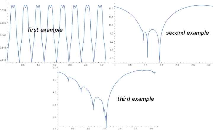
Figure 1. Graphs of the functions $\sum_{j=1}^{k}p_{j}\,\phi_{j}$

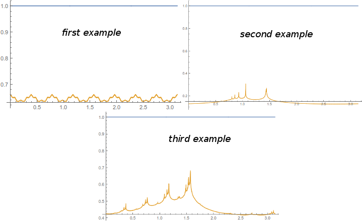
Figure 2. Graphs of the functions $H_{\alpha}(\underline{A})$

The numerics obtained are sinthesized in the following table. We stress again that these computations do not involve any kind of rigorous error control.

	$1^{{\rm st}}$ example	$2^{{\rm nd}}$ example	$3^{{\rm th}}$ example
$\alpha$	$0.5$	$0.1$	$0.1$
$\sigma_{\alpha}:=\max H_{\alpha}(\underline{A})$	$0.661033$	$0.67282$	$0.796829$
$N=\left|{\mathcal{F}}\right|$	$1000$	$512$	$512$
$\Delta_{\alpha}:=\Delta_{\alpha}(\underline{A},\mathcal{F})$	$0.0285419$	$0.517986656$	$0.499914$
$V_{\alpha}:=\sum_{j=1}^{k}p_{j}\,v_{\alpha}(\psi_{j})$	$0.284198$	$0.0403991$	$0.0642972$
$L_{1}(\underline{A},\mathcal{F})$	$0.8489$	$10.7506$	$4.56736$
$\Delta_{\alpha}\,(1-\sigma_{\alpha})^{-1}\,V_{\alpha}$	$0.0239301$	$0.0639592$	$0.158207$

Table 1. Computed data for the three examples. The last two rows represent the approximate LE and the estimated upper bound on the error.

8. Appendix: some projective inequalities

Consider the metric

$$\delta(\hat{x},\hat{y}):=\frac{\left\|x\wedge y\right\|}{\left\|x\right\|\left\|y\right\|}$$

on the projective space $\mathbb{P}(\mathbb{R}^{d})$, where $\hat{x}$ and $\hat{y}$ stand for projective classes of non-zero vectors $x,y\in\mathbb{R}^{d}$.

Given a point $\hat{x}\in\mathbb{P}(\mathbb{R}^{d})$ define the orthogonal projection $\pi_{\hat{x}}\colon\mathbb{R}^{d}\to\mathbb{R}^{d}$,

$$\pi_{\hat{x}}(v):=v-\left(v\cdot x\right)\,x$$

onto the hyperplane $x^{\perp}$, where $x\in\hat{x}$ is any unit vector representative of $\hat{x}$. Define also the (non linear) projection $\nu_{\hat{x}}\colon\mathbb{R}^{d}\to\mathbb{R}^{d}$,

$$\nu_{\hat{x}}(v):=\frac{\pi_{\hat{x}}(v)}{\left\|\pi_{\hat{x}}(v)\right\|}.$$

Given a matrix $A\in{\rm GL}_{d}(\mathbb{R})$, let $\Phi_{A}\colon\mathbb{P}(\mathbb{R}^{d})\to\mathbb{P}(\mathbb{R}^{d})$ be its projective action.

With the previous notation one has the following formula for the derivative of $\Phi_{A}$. For any $\hat{x}\in\mathbb{P}(\mathbb{R}^{d})$ and $v\in x^{\perp}=T_{\hat{x}}\mathbb{P}(\mathbb{R}^{d})$,

$$(D\Phi_{A})_{\hat{x}}(v)=\frac{\pi_{\Phi_{A}(x)}(A\,v)}{\left\|Ax\right\|}.$$ (13)

Remark 7.

Form the definition of derivative, given unit vectors $x,v\in\mathbb{R}^{d}$,

$$\lim_{\hat{y}\to\hat{x}}\frac{\delta(\Phi_{A}(\hat{x}),\Phi_{A}(\hat{y}))}{\delta(\hat{x},\hat{y})}=(D\Phi_{A})_{\hat{x}}(v)$$

where the limit is taken over the projective line $\mathrm{span}\{x,v\}\subset\mathbb{P}(\mathbb{R}^{d})$.

Proposition 9.

Given $\alpha>0$ and unit vectors $x,y\in\mathbb{R}^{d}$,

$$\left[\frac{\delta(\Phi_{A}(\hat{x}),\Phi_{A}(\hat{y}))}{\delta(\hat{x},\hat{y})}\right]^{\alpha} \leq\frac{1}{2}\,\left\{\left\|(D\Phi_{A})_{\hat{x}}(\nu_{\hat{x}}(y))\right\|^{\alpha}+\left\|(D\Phi_{A})_{\hat{y}}(\nu_{\hat{y}}(x))\right\|^{\alpha}\right\}$$

$$\leq\frac{1}{2}\,\left\{\left\|(D\Phi_{A})_{\hat{x}}\right\|^{\alpha}+\left\|(D\Phi_{A})_{\hat{y}}\right\|^{\alpha}\right\}.$$

Proof.

Given unit vectors $x,y\in\mathbb{R}^{d}$,

$$\left[\frac{\delta(\Phi_{A}(\hat{x}),\Phi_{A}(\hat{y}))}{\delta(\hat{x},\hat{y})}\right]^{\alpha} =\left[\frac{\left\|Ax\wedge Ay\right\|}{\left\|Ax\right\|\left\|Ay\right\|}\,\frac{1}{\left\|x\wedge y\right\|}\right]^{\alpha}$$

$$=\left[\frac{\left\|Ax\wedge Ay\right\|}{\left\|x\wedge y\right\|}\right]^{\alpha}\,\frac{1}{\left\|Ax\right\|^{\alpha}}\,\frac{1}{\left\|Ay\right\|^{\alpha}}$$

$$\leq\left[\frac{\left\|Ax\wedge Ay\right\|}{\left\|x\wedge y\right\|}\right]^{\alpha}\,\frac{1}{2}\,\left\{\frac{1}{\left\|Ax\right\|^{2\alpha}}+\frac{1}{\left\|Ay\right\|^{2\alpha}}\right\}$$

$$=\frac{1}{2}\,\left\{\left[\frac{\left\|Ax\wedge Ay\right\|}{\left\|x\wedge y\right\|}\right]^{\alpha}\,\frac{1}{\left\|Ax\right\|^{2\alpha}}+\left[\frac{\left\|Ax\wedge Ay\right\|}{\left\|x\wedge y\right\|}\right]^{\alpha}\,\frac{1}{\left\|Ay\right\|^{2\alpha}}\right\}$$

where we have used that $\sqrt{a\,b}\leq\frac{1}{2}\,\left\{a+b\right\}$ with $a=\left\|Ax\right\|^{-2\alpha}$ and $b=\left\|Ay\right\|^{-2\alpha}$. On the other hand for any non-zero vector $u\in\mathbb{R}^{d}$, because $\left\|u\wedge w\right\|$ is the area of the parallelogram spanned by $u$ and $w$, we must have $\left\|u\wedge w\right\|=\left\|u\right\|\,\left\|\pi_{\hat{u}}(w)\right\|$. Hence

$$\left\|\pi_{\hat{u}}(w)\right\|=\frac{\left\|u\wedge w\right\|}{\left\|u\right\|}.$$

Using this relation one has

$$\left\|(D\Phi_{A})_{\hat{x}}(\nu_{\hat{x}}(y))\right\| =\left\|(D\Phi_{A})_{\hat{x}}\left(\frac{\pi_{\hat{x}}(y)}{\left\|x\wedge y\right\|}\right)\right\|$$

$$=\frac{\left\|\pi_{\Phi_{A}(\hat{x})}\left(A\,\pi_{\hat{x}}(y)\right)\right\|}{\left\|Ax\right\|\,\left\|x\wedge y\right\|}=\frac{\left\|Ax\wedge A\,\pi_{\hat{x}}(y)\right\|}{\left\|Ax\right\|^{2}\,\left\|x\wedge y\right\|}$$

$$=\frac{\left\|Ax\wedge Ay\right\|}{\left\|Ax\right\|^{2}\,\left\|x\wedge y\right\|}.$$

Similarly, exchanging the roles of $x$ and $y$,

$$\left\|(D\Phi_{A})_{\hat{y}}(\nu_{\hat{y}}(x))\right\|=\frac{\left\|Ax\wedge Ay\right\|}{\left\|Ay\right\|^{2}\,\left\|x\wedge y\right\|}.$$

This establishes the proposition. ∎

Proposition 10.

Let $(\Omega,\mathscr{F},\mathbb{P})$ be a probability space, and $A\colon\Omega\to{\rm GL}_{d}(\mathbb{R})$ a matrix valued random variable. Then for any $\alpha>0$,

$$\sup_{\hat{x}\neq\hat{y}}\,\mathbb{E}\left[\left(\frac{\delta(\Phi_{A}(\hat{x}),\Phi_{A}(\hat{y}))}{\delta(\hat{x},\hat{y})}\right)^{\alpha}\right]=\sup_{\hat{x}\in\mathbb{P}(\mathbb{R}^{d})}\,\mathbb{E}\left[\,\left\|(D\Phi_{A})_{\hat{x}}\right\|^{\alpha}\,\right].$$

Proof.

For the first inequality ($\leq$) just average the one in Proposition 10 and then take sup. The converse inequality ($\geq$) follows from Remark 7. ∎

References

- [1] Philippe Bougerol, Théorèmes limite pour les systèmes linéaires à coefficients markoviens, Probab. Theory Related Fields 78 (1988), no. 2, 193–221. MR 945109
- [2] Pedro Duarte and Silvius Klein, Lyapunov exponents of linear cocycles; continuity via large deviations, Atlantis Studies in Dynamical Systems, vol. 3, Atlantis Press, 2016.
- [3] H. Furstenberg and H. Kesten, Products of random matrices, Ann. Math. Statist. 31 (1960), 457–469. MR 0121828
- [4] Harry Furstenberg, Noncommuting random products, Trans. Amer. Math. Soc. 108 (1963), 377–428. MR 0163345
- [5] by same author, Noncommuting random products, Trans. Amer. Math. Soc. 108 (1963), 377–428. MR 0163345
- [6] Stefano Galatolo, Maurizio Monge, and Isaia Nisoli, Rigorous approximation of stationary measures and convergence to equilibrium for iterated function systems, J. Phys. A 49 (2016), no. 27, 274001, 22. MR 3512100
- [7] Stefano Galatolo and Isaia Nisoli, An elementary approach to rigorous approximation of invariant measures, SIAM J. Appl. Dyn. Syst. 13 (2014), no. 2, 958–985. MR 3216642
- [8] Hubert Hennion and Loïc Hervé, Limit theorems for Markov chains and stochastic properties of dynamical systems by quasi-compactness, Lecture Notes in Mathematics, vol. 1766, Springer-Verlag, Berlin, 2001. MR 1862393 (2002h:60146)
- [9] Michael-R. Herman, Une méthode pour minorer les exposants de Lyapounov et quelques exemples montrant le caractère local d’un théorème d’Arnold et de Moser sur le tore de dimension , Comment. Math. Helv. 58 (1983), no. 3, 453–502. MR 727713
- [10] Émile Le Page, Régularité du plus grand exposant caractéristique des produits de matrices aléatoires indépendantes et applications, Ann. Inst. H. Poincaré Probab. Statist. 25 (1989), no. 2, 109–142. MR 1001021
- [11] Yuval Peres, Analytic dependence of Lyapunov exponents on transition probabilities, Lyapunov exponents (Oberwolfach, 1990), Lecture Notes in Math., vol. 1486, Springer, Berlin, 1991, pp. 64–80. MR 1178947
- [12] Mark Pollicott, Maximal Lyapunov exponents for random matrix products, Invent. Math. 181 (2010), no. 1, 209–226. MR 2651384
- [13] Frigyes Riesz and Béla Sz.-Nagy, Functional analysis, Frederick Ungar Publishing Co., New York, 1955, Translated by Leo F. Boron. MR 0071727
- [14] D. Ruelle, Analycity properties of the characteristic exponents of random matrix products, Adv. in Math. 32 (1979), no. 1, 68–80. MR 534172
- [15] Barry Simon and Michael Taylor, Harmonic analysis on and smoothness of the density of states in the one-dimensional Anderson model, Comm. Math. Phys. 101 (1985), no. 1, 1–19. MR 814540
- [16] Shlomo Sternberg, Lectures on differential geometry, Prentice-Hall, Inc., Englewood Cliffs, N.J., 1964. MR 0193578
- [17] P. Walters, An introduction to ergodic theory, Graduate Texts in Mathematics, Springer New York, 2000.