Formulas for Radial Transport in Protoplanetary Disks

Abstract

Quantification of the radial transport of gaseous species and solid particles is important to many applications in protoplanetary disk evolution. An especially important example is determining the location of the water snow lines in a disk, which requires computing the rates of outward radial diffusion of water vapor and the inward radial drift of icy particles; however, the application is generalized to evaporation fronts of all volatiles. We review the relevant formulas using a uniform formalism. This uniform treatment is necessary because the literature currently contains at least six mutually exclusive treatments of radial diffusion of gas, only one of which is correct. We derive the radial diffusion equations from first principles, using Fick’s law. For completeness, we also present the equations for radial transport of particles. These equations may be applied to studies of diffusion of gases and particles in protoplanetary and other accretion disks.

1 Introduction

One of the outstanding issues in studies of protoplanetary disks is the issue of radial mixing, both of gaseous species and particles with a range of sizes from microns to meters. Just a few examples of problems illustrate the importance of quantifying such radial diffusion. The Stardust mission discovered high-temperature condensates resembling fragments of chondrules and calcium-rich, aluminum-rich inclusions (CAIs), objects that formed at high temperatures indicative of an origin in the inner solar system, in the sample return from comet Wild 2, which must have formed in the outer solar system (Zolensky et al. 2006). Oxygen isotopic anomalies in meteorites are quite possibly carried by isotopically distinctive water formed in the outer solar system, radially advected inward as icy particles to the asteroid belt region (Lyons et al. 2009). There is evidence that enstatite chondrites record formation in a part of the solar nebula with elevated sulfur composition, possibly related to a sulfur snow line in which sulfur vapor diffuses outward beyond a condensation front (Pasek et al. 2005; Petaev et al. 2011). Finally, ${\rm H}_{2}{\rm O}$ snow lines are very important in our solar system for determining the water content of asteroids and planets. Just beyond the snow lines, outwardly diffusing water vapor can be cold-trapped as ice, enhancing the density of solid ice there, possibly triggering Jupiter’s formation (Stevenson & Lunine 1988; Cuzzi & Zahnle 2004). In each of these problems it is important to quantify how water or other vapor diffuses relative to the gas, as well as how particles of various sizes drift and diffuse relative to the gas.

The flow of matter through the disk is described by a formula for the time evolution of the surface density of gas, $\Sigma(r,t)$, which is a function of heliocentric distance $r$ and time $t$. This evolution can be written as two first-order differential equations for the viscous evolution of an accretion disk (Lynden-Bell & Pringle 1974). The first one describes the change in surface density $\Sigma$ as mass flows into and out of each annulus:

$$\frac{\partial\Sigma}{\partial t}=\frac{1}{2\pi r}\,\frac{\partial\dot{M}}{\partial r}=-\frac{1}{r}\,\frac{\partial}{\partial r}\left(r\,\Sigma\,V_{r}\right),$$ (1)

where $V_{r}=-\dot{M}/(2\pi r)$ is the average gas velocity (positive if outward). The second one describes the flow of mass due to the exchange of angular momentum between two adjacent annuli, coupled by a viscous torque mediated by turbulent viscosity $\nu$:

$$\dot{M}=6\pi\,r^{1/2}\,\frac{\partial}{\partial r}\left(r^{1/2}\,\Sigma\nu\right)=3\pi\Sigma\nu\left(1+2Q\right),$$ (2)

where $Q\equiv\partial\ln(\Sigma\nu)/\partial\ln r$ and $\dot{M}>0$ if the flow is inward. An important quantity is the radial velocity of the gas,

$$V_{r}=-\frac{\dot{M}}{2\pi r\Sigma}=-\frac{3\nu}{2r}\,\left(1+2Q\right).$$ (3)

(Inward gas flow has $V_{r}<0$.) Boundary conditions placed on $\dot{M}$ at inner and outer edges of the disk suffice to close the equations. One can also write these equations as a single second-order differential equation for $\Sigma$:

$$\frac{\partial\Sigma}{\partial t}=\frac{3}{r}\,\frac{\partial}{\partial r}\,\left[r^{1/2}\,\frac{\partial}{\partial r}\left(r^{1/2}\,\Sigma\nu\right)\right].$$ (4)

Self-similar solutions have been presented by Lynden-Bell & Pringle (1974) and Hartmann et al. (1998), and this treatment is standard in the literature.

What is sought is an additional formula that describes the evolution of the surface density of a tracer volatile, $\Sigma_{\rm c}$, or the evolution of the concentration of the volatile, $c\equiv\Sigma_{\rm c}/\Sigma$. Sometimes the volatiles are in the form of gas (vapor), or sometimes in the form of solid particles (e.g., icy grains) of potentially any size. In Section 2 we show that the literature currently contains multiple mutually exclusive formulas for the radial transport of gaseous tracer species, which are defined to be dynamically well coupled to the gas. In Section 3 we derive the correct formula from first principles using Fick’s law. In Section 4, for completeness, we provide a similar formula for the radial transport of solid particles. Finally, in section 5 we discuss the different outcomes predicted by various treatments, to illustrate the importance of using the correct formula. Our goal is to clear up the discrepancies in the literature and provide a resource for other researchers studying radial transport in accretion disks.

2 Existing Treatments of Gas Diffusion

Reviewing the literature, we found at least nine separate, original derivations that include six mutually exclusive differential equations describing how the concentration $c$ of a gaseous tracer species changes in time due to diffusion relative to the main gas in a protoplanetary disk. What defines a gaseous tracer species is that it is dynamically well coupled to the gas. This definition includes gaseous vapor, but could also apply to very small particles, as well. Here we review the various formulas for radial transport of gaseous tracer species, using a standardized formalism in which the radial velocity of the main gas is $V_{r}$, due to a turbulent viscosity $\nu$, and in which the tracer species diffuses relative to the gas with diffusion coefficient ${\cal D}_{\rm g}$. The mass diffusion coefficient of gas, ${\cal D}_{\rm g}$, and the kinematic viscosity $\nu$ are related but need not be identical; their ratio is the Schmidt number ${\rm Sc}=\nu/{\cal D}_{\rm g}$. We consider ${\cal D}_{\rm g}$ and $\nu$ to both vary with heliocentric distance.

2.1 Clarke & Pringle (1988), Gail (2001), Bockelée-Morvan et al. (2002)

Clarke & Pringle (1988), Gail (2001), and Bockelée-Morvan et al. (2002) each studied the problem of radial mixing in the same manner, apparently independently. Each started with the following equation, given by Morfill & Völk (1984):

$$\frac{\partial(c\rho)}{\partial t}+\nabla\cdot\left(c\,\rho\,\mbox{\boldmath$v$}\right)=\nabla\cdot\left(\rho{\cal D}_{\rm g}\,\nabla c\right)$$ (5)

(Gail 2001 cited Hirschfelder et al. 1964). Assuming axisymmetry, integrating this over all $z$, assuming $\rho(z)$ vanishes far from the midplane, and assuming $c$ and ${\cal D}_{\rm g}$ are vertically uniform, one derives:

$$\frac{\partial\Sigma_{\rm c}}{\partial t}+\frac{1}{r}\frac{\partial}{\partial r}\left(r\,\Sigma_{\rm c}\,V_{r}\right)=\frac{1}{r}\frac{\partial}{\partial r}\left(r\,\Sigma\,{\cal D}_{\rm g}\,\frac{\partial c}{\partial r}\right).$$ (6)

Likewise, one can vertically integrate the continuity equation,

$$\frac{\partial\rho}{\partial t}+\nabla\cdot\left(\rho\mbox{\boldmath$v$}\right)=0,$$ (7)

to find

$$\frac{\partial\Sigma}{\partial t}+\frac{1}{r}\frac{\partial}{\partial r}\left(r\,\Sigma\,V_{r}\right)=0.$$ (8)

Multiplying this equation by $c$ and subtracting from the previous one yields

$$\frac{\partial c}{\partial t}+V_{\rm r}\,\frac{\partial c}{\partial r}=\frac{1}{r\,\Sigma}\frac{\partial}{\partial r}\left(r\,\Sigma\,{\cal D}_{\rm g}\,\frac{\partial c}{\partial r}\right),$$ (9)

which is equivalent to equation 2.1.4 of Clarke & Pringle (1988), equation 12 of Gail (2001), and equation 4 of Bockelée-Morvan et al. (2002). We note that it is equivalent also to equation 21 of Cuzzi et al. (2003), who based their derivation on that of Bockelée-Morvan et al. (2002). If one assumes ${\rm Sc}=1$, one can write

$$\frac{\partial c}{\partial t}=\nu\left[(\frac{5}{2}+4Q)\,\frac{1}{r}\frac{\partial c}{\partial r}+\frac{\partial^{2}c}{\partial r^{2}}\right].$$ (10)

2.2 Stevenson & Lunine (1988)

Stevenson & Lunine (1988) started with the equation

$$\frac{\partial c}{\partial t}+V_{\rm r}\,\frac{\partial c}{\partial r}=\frac{{\cal D}_{\rm g}}{r}\,\frac{\partial}{\partial r}\left(r\frac{\partial c}{\partial r}\right)$$ (11)

(their equation 6), then argued that $V_{\rm r}\approx-\nu/r\approx-{\cal D}_{\rm g}/r$ on dimensional grounds, to derive a simplified formula. Their treatment captures the physics of the problem but neglects the effects of any radial gradients in the density and the diffusion coefficient. Assuming ${\rm Sc}=1$, it is straightforward to show this equation can be rewritten:

$$\frac{\partial c}{\partial t}=\nu\left[(\frac{5}{2}+3Q)\,\frac{1}{r}\frac{\partial c}{\partial r}+\frac{\partial^{2}c}{\partial r^{2}}\right].$$ (12)

2.3 Drouart et al. (1999)

A different treatment was adopted by Drouart et al. (1999), who wrote:

$$\frac{\partial c}{\partial t}+\frac{1}{r}\,\frac{\partial}{\partial r}\,\left(r\,V_{r}\,c\right)=\frac{1}{r\,\Sigma}\,\frac{\partial}{\partial r}\,\left(r\,\Sigma\,{\cal D}_{\rm g}\,\frac{\partial c}{\partial r}\right)$$ (13)

(their equation 9). This can be rewritten as

$$\frac{\partial\Sigma_{\rm c}}{\partial t}+\frac{1}{r}\,\frac{\partial}{\partial r}\,\left(r\,V_{r}\,\Sigma_{\rm c}\right)+\Sigma_{\rm c}\,\frac{1}{r}\,\frac{\partial}{\partial r}\,\left(rV_{r}\right)=\frac{1}{r}\,\frac{\partial}{\partial r}\,\left(r\,\Sigma\,{\cal D}_{\rm g}\,\frac{\partial c}{\partial r}\right).$$ (14)

Assuming ${\rm Sc}=1$, we can also write this as

$$\frac{\partial c}{\partial t}=-c\,\left(\frac{V_{r}}{r}+\frac{\partial V_{r}}{\partial r}\right)+\nu\,\left[\left(\frac{5}{2}+4Q\right)\,\frac{1}{r}\frac{\partial c}{\partial r}+\frac{\partial^{2}c}{\partial r^{2}}\right].$$ (15)

This differs from other treatments by including a term proportional to the concentration and the divergence of the velocity field, erroneously implying that the concentration would increase if the density were to increase.

2.4 Cuzzi & Zahnle (2004)

The treatment of Cuzzi & Zahnle (2004) is similar but not quite identical. Setting $f_{\rm L}=0$ in their equations 1 and 2 yields

$$\frac{\partial c}{\partial t}=V_{{\rm r}}\,\frac{\partial c}{\partial r}+\frac{1}{r\Sigma}\,\frac{\partial}{\partial r}\,\left[{\cal D}_{\rm g}\,\frac{\partial}{\partial r}\left(c\Sigma\right)\right].$$ (16)

This resembles the equations derived by Clarke & Pringle (1988) and others, but includes several extra terms involving the gradients of $\Sigma$ and ${\cal D}_{\rm g}$.

2.5 Ciesla & Cuzzi (2006) and Guillot & Hueso (2006)

Two later treatments started with different equations but apparently a common starting assumption. Ciesla & Cuzzi (2006) wrote

$$\frac{\partial\Sigma_{\rm c}}{\partial t}=\frac{3}{r}\,\frac{\partial}{\partial r}\left[r^{1/2}\,\frac{\partial}{\partial r}\left(\Sigma_{\rm c}\,\nu\,r^{1/2}\right)\right]$$ (17)

(their equation 11), apparently deriving their equations by assuming $\Sigma_{\rm c}$ would evolve by the same differential equation as $\Sigma$. Guillot & Hueso (2006) wrote

$$\frac{\partial c}{\partial t}=3\nu\left[\left(\frac{3}{2}+2\frac{\partial\ln(\Sigma\nu)}{\partial\ln r}\right)\,\frac{1}{r}\frac{\partial c}{\partial r}+\frac{\partial^{2}c}{\partial r^{2}}\right]$$ (18)

(their equation 5). It is straightforward to show that these are equivalent, and both can be rewritten (again assuming ${\rm Sc}=1$) as

$$\frac{\partial c}{\partial t}=3\nu\left[(\frac{3}{2}+2Q)\,\frac{1}{r}\frac{\partial c}{\partial r}+\frac{\partial^{2}c}{\partial r^{2}}\right].$$ (19)

It is notable that in this treatment the diffusion coefficient is $3\nu$, not the value $\nu$ that should obtain in the limit of small spatial scales.

2.6 Ciesla (2009)

Ciesla (2009) derived a diffusion equation starting with the two-dimensional formula

$$\frac{\partial c}{\partial t}+\frac{1}{r\,\rho}\,\frac{\partial}{\partial r}\left(rV_{r}\rho c\right)+\frac{1}{\rho}\frac{\partial}{\partial z}\left(V_{z}\rho c\right)=\frac{1}{r\,\rho}\frac{\partial}{\partial r}\left(r\rho\nu\frac{\partial c}{\partial r}\right)+\frac{1}{\rho}\frac{\partial}{\partial z}\left(\rho\nu\frac{\partial c}{\partial z}\right)$$ (20)

(his equation 9), which is equivalent to

$$\frac{\partial c}{\partial t}+\frac{1}{\rho}\nabla\cdot\left(\rho c\mbox{\boldmath$v$}\right)=\frac{1}{\rho}\nabla\cdot\left(\rho\nu\nabla c\right),$$ (21)

assuming axisymmetry. In the same manner as before this can be converted to a one-dimensional form, by integrating over all $z$, and assuming $\nu$ and $c$ are vertically uniform. One finds

$$\frac{\partial c}{\partial t}+\frac{1}{r\,\Sigma}\frac{\partial}{\partial r}\left(r\,\Sigma\,V_{r}\,c\right)=\frac{1}{r\,\Sigma}\frac{\partial}{\partial r}\left(r\,\Sigma\,\nu\,\frac{\partial c}{\partial r}\right).$$ (22)

This differs from previous treatments in that the product $r\Sigma V_{\rm r}$ is inside the radial derivative on the left-hand side. This formula can be rewritten as

$$\frac{\partial c}{\partial t}=\frac{c}{\Sigma}\,\frac{\partial\Sigma}{\partial t}+\nu\left[\left(\frac{5}{2}+4Q\right)\,\frac{1}{r}\frac{\partial c}{\partial r}+\frac{\partial^{2}c}{\partial r^{2}}\right].$$ (23)

This is identical to the formula of Gail (2001) except for the term $(c/\Sigma)\,\partial\Sigma/\partial t$ on the left-hand side, which erroneously assumes that the concentration would change if the surface density were to change (as was also assumed by Drouart et al. 1999).

3 Derivation of Gas Diffusion Equation

To determine which (if any) of the above equations is correct, we derive the volatile radial diffusion equation from first principles. A tracer species will be advected with the gas, even as it diffuses relative to it. We assign an effective mass accretion rate to the species $c$, which is the sum of the flux due to its advection in the mean flow, and the diffusion flux due to concentration gradients, following Fick’s law:

$$\frac{\partial}{\partial t}\left(\rho c\right)=-\nabla\cdot\mbox{\boldmath$F$},$$ (24)

where the flux of the tracer species is

$$\mbox{\boldmath$F$}=\rho c\,\mbox{\boldmath$v$}-{\cal D}_{\rm g}\,\rho\,\nabla c,$$ (25)

the first term being an advective term and the second term capturing diffusion of the tracer relative to the gas. Again integrating over $z$ and assuming ${\cal D}_{\rm g}$, $c$ and $V_{r}$ are vertically uniform, we find

$$\frac{\partial}{\partial t}\,\left(\Sigma c\right)+\frac{1}{r}\,\frac{\partial}{\partial r}\,\left(r\,\Sigma\,c\,V_{r}\right)=\frac{1}{r}\,\frac{\partial}{\partial r}\,\left(r\,{\cal D}_{\rm g}\,\Sigma\,\frac{\partial c}{\partial r}\right).$$ (26)

Clarke & Pringle (1988) started with this equation [their equation 2.1.4], deriving it from the contaminant equation given by Morfill & Völk (1984). We believe that Morfill & Völk (1984) are the first to write this (correct) three-dimensional equation in the context of protoplanetary disks. This equation is equivalent to setting the mass flux of the tracer species to

$$\dot{M}_{\rm c}=c\,\dot{M}+2\pi r\,{\cal D}_{\rm g}\,\Sigma\,\frac{\partial c}{\partial r},$$ (27)

where ${\cal D}_{\rm g}$ is the diffusion coefficient of species $c$ through the main gas. The sign of the diffusion flux means that species $c$ diffuses inward (positive $\dot{M}_{\rm c}$) if $\partial c/\partial r>0$. We then write

$$\frac{\partial}{\partial t}\left(c\Sigma\right)=\frac{1}{2\pi r}\,\frac{\partial\dot{M}_{\rm c}}{\partial r},$$ (28)

or

$$c\frac{\partial\Sigma}{\partial t}+\Sigma\frac{\partial c}{\partial t}=\frac{1}{2\pi r}\,\frac{\partial}{\partial r}\left[c\dot{M}+2\pi r{\cal D}_{\rm g}\Sigma\frac{\partial c}{\partial r}\right].$$ (29)

If we impose $c\equiv 1$ we recover

$$\frac{\partial\Sigma}{\partial t}=\frac{1}{2\pi r}\,\frac{\partial\dot{M}}{\partial r},$$ (30)

as expected. Subtracting $c$ times this equation yields

$$\frac{\partial c}{\partial t}=\frac{1}{2\pi r}\frac{\dot{M}}{\Sigma}\,\frac{\partial c}{\partial r}+\frac{1}{r\,\Sigma}\frac{\partial}{\partial r}\left[r\,\Sigma{\cal D}_{\rm g}\,\frac{\partial c}{\partial r}\right].$$ (31)

We replace $\dot{M}$ with $3\pi\Sigma\nu(1+2Q)$ to find

$$\frac{\partial c}{\partial t}=\frac{3}{2}\frac{\nu}{r}(1+2Q)\,\frac{\partial c}{\partial r}+\frac{{\cal D}_{\rm g}}{r}\,(1+Q^{\prime})\,\frac{\partial c}{\partial r}+{\cal D}_{\rm g}\,\frac{\partial^{2}c}{\partial r^{2}},$$ (32)

where $Q^{\prime}\equiv\partial\ln(\Sigma{\cal D}_{\rm g})/\partial\ln r$. Substituting ${\cal D}_{\rm g}=\nu/{\rm Sc}$,

$$\frac{\partial c}{\partial t}=\nu\left[\left(\frac{3}{2}(1+2Q)+\frac{(1+Q^{\prime})}{{\rm Sc}}\right)\,\frac{1}{r}\frac{\partial c}{\partial r}+\frac{1}{\rm Sc}\,\frac{\partial^{2}c}{\partial r^{2}}\right].$$ (33)

Note that the roles of diffusion (dependent on ${\cal D}_{\rm g}$ and advection (affected by the gas velocity, and therefore $\nu$) are separated. Equation 33 is the proper equation to track the radial evolution of gas-phase volatiles in protoplanetary disks. We note that it is more general than many existing treatments, and clearly delineates the effect of the Schmidt number not equal to unity.

For most normal solar nebula turbulent flows, it is very likely that the Schmidt number is constant at ${\rm Sc}\approx 0.7$ (e.g., Launder 1976, McComb 1990; Johansen et al. 2007; Hughes & Armitage 2010). In the limit ${\rm Sc}=1$,

$$\frac{\partial c}{\partial t}=\nu\left[(\frac{5}{2}+4Q)\,\frac{1}{r}\frac{\partial c}{\partial r}+\frac{\partial^{2}c}{\partial r^{2}}\right],$$ (34)

which matches the equations derived by Clarke & Pringle (1988), Gail (2001), and Bockelée-Morvan et al. (2002).

In summary, we found six different, mutually exclusive equations in the literature to describe the diffusion of gas in protoplanetary disks. We advocate use of the most general form, Equation 33 above, which works for arbitrary Schmidt number. In the limit ${\rm Sc}=1$, this equation matches those of Clarke & Pringle (1988), Gail (2001), Bockelée-Morvan et al. (2002), and Cuzzi et al. (2003). Even in the limiting case ${\rm Sc}=1$, other treatments differ.

4 Radial Diffusion and Drift of Particles

Calculating the radial transport of solids is just as fundamental a problem as calculating the radial transport of gases. While very small ($\sim$ micron-sized) particles have the same transport properties as gas, the transport of larger particles is more complicated, because such particles not only are advected and diffuse relative to the gas, they also can drift relative to the gas. The basis for particle drift is that gas in a protoplanetary disk, being partially supported against gravity by a pressure gradient force, orbits the star with a velocity less than the Keplerian velocity; particles, which try to maintain an orbit at Keplerian velocity around the star, feel a headwind that makes them lose angular momentum and spiral in toward the star. For completeness, we discuss various approaches to the calculation of these effects.

The radial transport of particles is governed by the same general formulas as the gas is. Defining the concentration of solid particles as $c\equiv\Sigma_{\rm c}/\Sigma$, one again has

$$\frac{\partial}{\partial t}\left(c\Sigma\right)=\frac{1}{2\pi r}\,\frac{\partial\dot{M}_{\rm c}}{\partial r},$$ (35)

as in Equation 27 for the gas, but where the mass accretion rate associated with particles includes advection, diffusion, and drift. One approach is to treat particles exactly as a gaseous fluid, with $\dot{M}_{\rm c}$ defined as Equation 26, but with an additional term for drift at velocity $\delta u$ with respect to the gas, so that

$$\dot{M}_{\rm c}=c\dot{M}-2\pi r\,c\Sigma\,\left(\Delta u\right)+2\pi r\,{\cal D}_{\rm p}\,\Sigma\,\frac{\partial c}{\partial r}$$ (36)

(here we assume $\Delta u<0$ if particles drift inward, making $\dot{M}_{\rm c}$ more positive). Equivalently,

$$\dot{M}_{\rm c}=-2\pi r\,c\Sigma\,\left[-V_{r}+\Delta u\right]+2\pi r\,{\cal D}_{\rm p}\,\Sigma\,\frac{\partial c}{\partial r},$$ (37)

where $V_{r}+\Delta u$ represents the total radial velocity of the particles.

To calculate the total radial velocity of the particles, we favor the approach of Takeuchi & Lin (2002) [see also Nakagawa et al. (1986), Birnstiel et al. (2010), and Estrada et al. (2016)], which we reproduce here. Gas orbits the star with an angular velocity $\Omega=\Omega_{\rm K}\,\left(1-\eta\right)^{1/2}$, where $\eta=-(r\Omega_{\rm K}^{2})^{-1}\rho_{\rm g}^{-1}\,\partial P_{\rm g}/\partial r$ $\sim 10^{-3}$, $\rho_{\rm g}$ and $P_{\rm g}$ are the gas density and pressure, and $\Omega_{\rm K}$ the Keplerian orbital frequency. The gas has velocity $V_{{\rm g},\phi}=r\Omega$ in the azimuthal direction and $V_{{\rm g},r}$ in the radial direction. Particles have azimuthal velocity $V_{{\rm p},\phi}$ and radial velocity $V_{{\rm p},r}$ that differ from the gas velocity, and therefore paticles experience a drag force. The radial component of the force equation is

$$\frac{dV_{{\rm p},r}}{dt}=\frac{V_{\rm p,\phi}^{2}}{r}-\Omega_{\rm K}^{2}r-\frac{1}{t_{\rm stop}}\,\left(V_{{\rm p},r}-V_{{\rm g},r}\right),$$ (38)

where $t_{\rm stop}$ is the aerodynamic stopping time, defined by matching the acceleration from the drag force to the term above. Likewise, particles lose angular momentum due to the aziumthal drag force:

$$\frac{d}{dt}\,\left(rV_{{\rm p},\phi}\right)=-\frac{1}{t_{\rm stop}}\,\left(V_{{\rm p},\phi}-V_{{\rm g},\phi}\right).$$ (39)

Using $t_{\rm stop}$, we define the Stokes number as the product of orbital frequency and aerodynamic stopping time:

$${\rm St}=\Omega_{\rm K}\,t_{\rm stop}.$$ (40)

In the special case of particles smaller than the molecular mean free path (Epstein limit), the aerodynamic stopping time and Stokes number can be written in terms of particle properties as

$${\rm St}=\Omega_{\rm K}\,\frac{\rho_{\rm p}a}{\rho_{\rm g}C_{\rm s}},$$ (41)

where $\rho_{\rm p}$ and $a$ are the particle density and radius, and $C_{\rm s}$ the sound speed, appropriate for particles smaller than the molecular mean free path (Weidenschilling 1977; Cuzzi & Weidenschilling 2006). For particles with radius $a=1\,{\rm mm}$, at 1 AU, assuming $\rho_{\rm g}=10^{-9}\,{\rm g}\,{\rm cm}^{-3}$ and $C_{\rm s}\sim 1\,{\rm km}\,{\rm s}^{-1}$, ${\rm St}\sim 10^{-3}$. In the limit of small particles, such that ${\rm St}\ll 1$, Takeuchi & Lin (2002) find a solution; assuming $V_{{\rm g},\phi}\approx V_{{\rm p},\phi}\approx r\,\Omega_{\rm K}$, they find

$$V_{{\rm p},r}=\frac{V_{{\rm g},r}-\eta\,{\rm St}\,r\,\Omega_{\rm K}}{1+{\rm St}^{2}}.$$ (42)

The drift speed in this case is

$$\Delta u=V_{{\rm p},r}-V_{{\rm g},r}=\frac{-{\rm St}^{2}\,V_{{\rm g},r}-\eta\,{\rm St}\,r\,\Omega_{\rm K}}{1+{\rm St}^{2}},$$ (43)

which is generally negative (inward), and which vanishes for small particles. For millimeter-sized particles, with ${\rm St}\approx 10^{-3}$, the drift speed at 1 AU is $\approx\,V_{{\rm g},r}-\eta\,{\rm St}\,r\Omega_{\rm K}$, both terms being of order $\sim 10^{-6}\,{\rm AU}\,{\rm yr}^{-1}$.

Weidenschilling (1977) derived a formula for the drift speed starting with the same assumptions, but valid for particles of all sizes, not just small particles in the Epstein regime. He showed that meter-sized particles would drift inward very rapidly, at rates $\sim\,10^{-2}\,{\rm AU}\,{\rm yr}^{-1}$, orders of magnitude greater than the drift rate of millimeter-sized particles. Unfortunately, in the small-particle limit, the calculation of Weidenschilling (1977) does not reproduce that of Takeuchi & Lin (2002): when relating the loss of angular momentum to the radial velocity of particles (Weidenschilling’s Equation 19), it is assumed that particles have radial velocity $\Delta u$ instead of $\Delta u+V_{{\rm g},r}$. While this approximation is appropriate for rapidly drifting particles (or a disk with no radial flow), it is not appropriate for small particles for which $\left|\Delta u\right|\,\sim\,\left|V_{{\rm g},r}\right|$. We therefore prefer the formulation of Takeuchi & Lin (2002) to account for the particle advection and drift.

The last term to modify for radial transport of particles is the diffusion term. Vapor and very small particles diffuse relative to the gas with diffusion coefficient ${\cal D}_{\rm g}$ that differs from the turbulent viscosity $\nu$ by a factor equal to the Schmidt number: ${\cal D}_{\rm g}=\nu\,{\rm Sc}^{-1}$. Larger particles will diffuse a rate that differs from this value, depending on their aerodynamic stopping time and the level of turbulence. We adopt the relationship

$${\cal D}_{\rm p}=\frac{{\cal D}_{\rm g}}{1+{\rm St}^{2}}=\frac{\nu\,{\rm Sc}^{-1}}{1+{\rm St}^{2}}.$$ (44)

(Youdin & Lithwick 2007; Carballido et al. 2011). It will be convenient to define a new quantity

$$Q^{\prime}_{\rm p}\equiv\frac{r}{\Sigma{\cal D}_{\rm p}}\,\frac{\partial}{\partial r}\,\left(\Sigma{\cal D}_{\rm p}\right),$$ (45)

analogous to the similar quantity $Q^{\prime}$ involving ${\cal D}$.

Combining the above equations, we derive a differential equation for $c$, the concentration of particles:

$$\frac{\partial c}{\partial t}=\nu\,\left[\left(\frac{3}{2}\left(1+2Q\right)+\frac{\left(1+Q^{\prime}_{\rm p}\right)}{{\rm Sc}\,(1+{\rm St}^{2})}\right)\,\frac{1}{r}\frac{\partial c}{\partial r}+\frac{1}{{\rm Sc}(1+{\rm St}^{2})}\,\frac{\partial^{2}c}{\partial r^{2}}\right]-\frac{1}{r\Sigma}\,\frac{\partial}{\partial r}\,\left[r\,\left(\Delta u\right)\,c\Sigma\right]$$

Because the drift speed $\Delta u$ can vary in a complicated way with particle size and position in the disk, we do not attempt to generalize this equation further. For a more detailed discussion of the transport of particles with arbitrary stopping times, and the role of the Schmidt number, see Estrada et al. (2016), whose equation 11 is consistent with our Equations 33 and 46.

Among other treatments in the literature of the radial transport of particles, we find that the treatment of Birnstiel et al. (2010) is essentially identical to the treatment presented here. We note that the treatment of Brauer et al. (2008) follows essentially the same lines, but assumes the diffusion coefficient of particles is ${\cal D}_{\rm p}={\cal D}_{\rm g}\,(1+{\rm St})^{-1}$, following Völk et al. (1980), Cuzzi et al. (1993) and Schräpler & Henning (2004), instead of the form we prefer here, following Youdin & Lithwick (2007) and Carballido et al. (2011). Our treatment differs from that of Stepinski & Valageas (1996, their equation 18), which resembles the treatment of Guillot & Hueso (2002) and Ciesla & Cuzzi (2006) for gas diffusion, as described above.

5 Discussion

Radial transport of gaseous volatiles and solid particles is a problem that arises often in studies of accretion disks, especially in studies of snow lines in protoplanetary disks. Given the fundamental importance of volatile transport, it is unfortunate that so many discrepant treatments of it exist in the literature. The various formulas appear similar in form, but in fact they can predict quite different results. In this section we explore in detail some implications of the use of different volatile transport formulations in modeling disk evolution, using a simple $\alpha$ disk model to demonstrate disk behavior under varying turbulent strengths using three different volatile treatments. In addition, we also use water as our tracer species, and explore the effects that each treatment has on the total water abundance across the disk.

5.1 Effects of Diffusion in a Uniform $\alpha$-disk

To illustrate the effects of diffusion, we perform simulations of simple $\alpha$ disks that incorporate three different formulations for volatile transport: i) the treatment used in our work [also that of Clarke & Pringle (1988), Gail (2001), and Bockelée-Morvan et al. (2002)]; ii) the treatment of Guillot & Hueso (2006) and Ciesla & Cuzzi (2006) [hereafter GH06/CC06]; and iii) Stevenson & Lunine (1988) [hereafter SL88]. The results of the above simulations are shown with the evolution of a dye, initially placed in an annulus between 1 and 2 AU at time $t=0$, at times $t=0.1\,{\rm Myr}$ and $t=1\,{\rm Myr}$, using the three different formulations. Disk simulations are performed using the following values of $\alpha$: 10^-4, 10^-3 and 10^-2.

The underlying evolution of the disk is determined by assuming $\nu=\alpha c_{\rm s}^{2}\Omega^{-1}$, where $c^{2}_{\rm s}=(kT/\bar{m})$ is the sound speed, $T(r)=100\,(r/1\,{\rm AU})^{-1/2}\,{\rm K}$ the disk temperature, $r$ the heliocentric distance, and $\bar{m}=2.33\,m_{\rm p}$ the mean molecular weight. The initial surface density is $\Sigma(r)\approx 6000\,(r/1\,{\rm AU})^{-3/2}\,{\rm g}\,{\rm cm}^{-2}$, as per Kalyaan et al. (2015). Photoevaporation due to the minimum plausible irradiation by an external ultraviolet field ($G_{0}=0.1$) is assumed. We thereafter numerically calculate the evolution of the disk using the treatment of Kalyaan et al. (2015). For the alternate formulations tested here, we converted the original $\Sigma_{c}$ evolution equations of GH06/CC06 and SL88 to a mass accretion rate $\dot{M_{c}}$ for implementation into our code. This required us to assume that $(1/r)\partial(\Sigma D)/\partial r=0$ (i.e., $Q^{\prime}=0$) in order to make the differential equation easily solvable. Therefore in all cases of the alternative treatments, we use identical $\Sigma D$, fixed at value at 1 AU so that $Q^{\prime}=0$. These equations are as follows. For GH06/CC06,

$$\dot{M}_{\rm c}=c\,\dot{M}+6\pi r\,\left(\Sigma{\cal D}\right)\,\frac{\partial c}{\partial r};$$ (46)

for SL88,

$$\dot{M}_{\rm c}=c\,\dot{M}-\pi c\Sigma{\cal D}\,+2\pi r\,\left(\Sigma{\cal D}\right)\,\frac{\partial c}{\partial r};$$ (47)

and for comparison, the equation we use is

$$\dot{M}_{\rm c}=c\,\dot{M}+2\pi r\,\left(\Sigma{\cal D}\right)\,\frac{\partial c}{\partial r}.$$ (48)

Figures 1, 2 and 3 show results of our simulations for intermediate ($\alpha=10^{-3}$), low ($\alpha=10^{-4}$) and high ($\alpha=10^{-2}$) values of $\alpha$. Figure 1 ($\alpha=10^{-3}$) illustrates that the different treatments predict very different volatile concentrations in the outer protoplanetary disk for $\alpha=10^{-3}$. At 10 AU, after 0.1 Myr, the concentration should be $3\times 10^{-8}$, and at 1 Myr it should be $8\times 10^{-4}$. The treatment of Stevenson & Lunine (1988) predicts values of $2\times 10^{-7}$ and $\approx 1.5\times 10^{-3}$. The treatments of Guillot & Hueso (2006) and Ciesla & Cuzzi (2006) predict values of $2\times 10^{-4}$ and $\approx 3\times 10^{-3}$. Use of the incorrect equation can overestimate the volatile concentration by orders of magnitude. Figure 2 ($\alpha=10^{-4}$) illustrates that the GH06/CC06 equations show diffusion of vapor is enhanced by several orders of magnitude both inward and outward of the annulus, at both 0.1 and 1 Myr. At 4 AU, GH06/CC06 predicts $c$ = 1 $\times$ 10^-4 at 0.1 Myr and 8 $\times$ 10^-1 at 1 Myr. In contrast, SL88 and our work predict similar concentrations of 1 $\times$ 10^-8 at 0.1 Myr and $\sim$ 4 $\times$ 10^-3 at 1 Myr. In Figure 3 ($\alpha=10^{-2}$), it is seen that high $\alpha$ leads to greater turbulent mixing in disks, leading to largely similar profiles, deviating in only factors of a few. Our treatment predicts $c$ = 6 $\times$ 10^-3 at 0.1 Myr, and $\approx$ 3 $\times$ 10^-4 at 1 Myr, at 1 AU. For comparison, GH06/CC06 predict 6 $\times$ 10^-3 (same as ours) and $\approx$ 2 $\times$ 10^-3, and SL88 predict 1 $\times$ 10^-2 and 1 $\times$ 10^-3.

As expected, the choice of the treatment for volatile transport is more significant for disks with lower $\alpha$, but for reasonable values of $\alpha$, pertinent to weakly turbulent midplanes of protoplanetary disks, using the correct treatment is clearly critical to accurately predicting volatile transport.

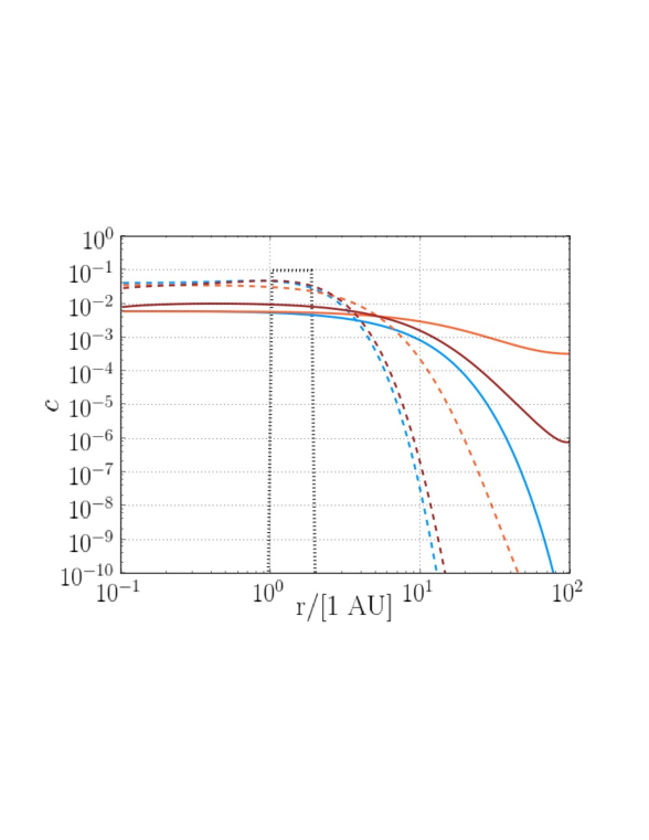
Figure 1: Simulated evolution over time of the concentration, $c(r)$, of a tracer volatile, using three different formulas to describe the radial transport. All three cases begin with the same initial concentration: $c(r)=0.1$ between 1 and 2 AU (dotted lines) and have turbulent viscosity $\alpha=10^{-3}$. The blue curves show the $c(r)$ at 0.1 Myr (dashed) and 1 Myr (solid) using the formula we suggest (cf. Gail 2001). The orange curves likewise show the evolution using the equation of Guillot & Hueso (2006) and Ciesla & Cuzzi (2006), and the brown curves show the evolution using the equation of Stevenson & Lunine (1988). These two formulations tend to overestimate the amount of diffusion that occurs.

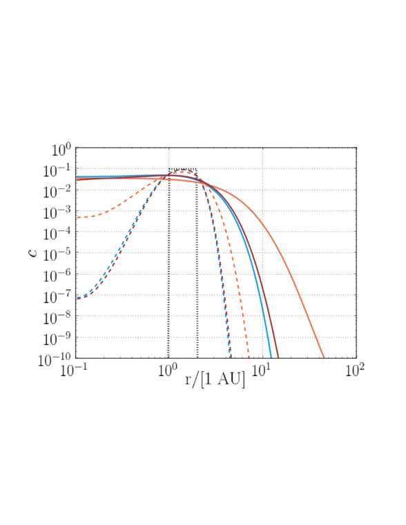
Figure 2: Simulated evolution over time of the concentration, $c(r)$, of a tracer volatile using different radial transport formulas. Same as Figure 1, but for disks with lower turbulent viscosity, $\alpha$ = 10^-4 . GH06/CC06 are seen to overestimate volatile diffusion in disks with low $\alpha$.

Figure 3: Simulated evolution over time of the concentration, $c(r)$, of a tracer volatile using different radial transport formulas. Same as Figure 1, but for disks with higher turbulent viscosity, $\alpha$ = 10^-2. GH06/CC06 and SL88 both predict slightly faster volatile diffusion in disks with high $\alpha$.

5.2 Radial Water Abundance Across the Snow Line

As a second illustration of the effects of the different formulas, for a case with particle transport, we build on the above disk model and include both volatile and particle transport, to determine the water ice-to-rock ratio across the disk. We use our multi-fluid code to track each of the following fluids: bulk disk gas ($\Sigma_{g}$); water vapor ($\Sigma_{\rm vap}$); ‘icy’ chondrules composed entirely of water ice ($\Sigma_{\rm icychondrules}$); ‘rocky’ chondrules composed of silicates ($\Sigma_{\rm rockychondrules}$); icy asteroids that grow by accreting icy chondrules ($\Sigma_{\rm icyast}$); and rocky asteroids that grow by accreting ‘rocky’ chondrules ($\Sigma_{\rm rockyast}$). Further details will be presented by Kalyaan et al. (2017 in prep.). Uniform tracer concentrations $c(r)\sim$ 10^-4 for each component are assumed initially throughout the disk. Both ‘icy’ and ‘rocky’ chondrules are assumed to be small solid particles of 1 mm diameter and have the same initial uniform surface density throughout the disk, $5\times 10^{-3}\,\Sigma_{\rm gas}$.

Throughout the disk’s evolution, both icy and rocky chondrules radially drift inwards in the disk according to Equation 43. Icy chondrules are additionally influenced by the change of phase of water ice to vapor at pressure and temperature conditions close to the snow line region. To determine what phase of water exists at a given location, we first use the following equations to determine the saturation water vapor pressure over ice at each radius $r$. For $T>169\,$K, we use the formulation from Marti & Mauersberger (1993),

$$P_{\rm vap}(R)=0.1\,\exp\,\left(28.868-\frac{6132.9\,{\rm K}}{T}\right)\,{\rm dyn}\,{\rm cm}^{-2}$$ (49)

while for $T<169\,{\rm K}$ we use the formulation from Mauersberger & Krankowsky (2003):

$$P_{\rm vap}(R)=0.1\,\exp\,\left(34.262-\frac{7044.0\,{\rm K}}{T}\right)\,{\rm dyn}\,{\rm cm}^{-2}.$$ (50)

We assume that the above formulation for $T\,<\,169\,$K (Mauersberger & Krankowsky, 2003) is sufficiently accurate when extrapolated to lower temperatures ($\sim$150K), as the authors suggest. The surface density equivalent of $P_{\rm vap}$ is then calculated as

$$\Sigma_{H_{2}O,{\rm eq}}(T)=\sqrt{2\pi}\,\left(\frac{P_{\rm vap}}{c_{s}^{2}}\right).$$ (51)

The densities of vapor and ice in this condensation-evaporation region are then determined as follows. If $\Sigma_{H_{2}O,{\rm vap}}(T)$ exceeds the total water content (excluding water already accreted into asteroids) at radius $r$ (i.e., $\Sigma_{\rm vap}$ $+$ $\Sigma_{\rm icy\,chondrules}$), we assume that all of the water is converted into vapor. If on the other hand, $\Sigma_{H_{2}O,vap}(T)$ is less than the total water content (excluding water in asteroids), then we assume that $\Sigma_{\rm vap}$ = $\Sigma_{H_{2}O,{\rm eq}}$, and the remaining water is in water ice. Asteroids are assumed to grow from chondrules at a timescale $t_{\rm growth}$ $\sim$ 1 Myr and behave as a sink for water beyond the snow line, as follows:

$$\frac{\partial\Sigma_{\rm icyast}}{\partial t}=\frac{\Sigma_{\rm icy\,chondrules}}{t_{\rm growth}}$$ (52)

Radial drift of asteroids and their migration is ignored in this study.

We have incorporated the different diffusion formulations into an $\alpha$-disk model as in §5.1, with radial particle transport and condensation-evaporation of volatiles as described above, along with accretional heating. Following Lesniak & Desch (2011), this model assumes that accretion is dominant only in the active surface layers of the disk, whose surface density is assumed to be $\Sigma_{\rm act}$ $\sim 10\,{\rm g}\,{\rm cm}^{-2}$, for which the optical depth through the active layer is $\tau=\kappa\,\Sigma_{\rm active}$, where $\kappa=10\,{\rm cm}^{2}\,{\rm g}^{-1}$. Thereafter, the midplane temperature is calculated as follows:

$$\sigma T^{4}_{\rm mid}\approx\sigma T^{4}_{\rm passive}+\frac{27}{32}\,\Sigma_{\rm act}\nu_{\rm act}\Omega^{2}\,\tau$$ (53)

Here, $\nu_{\rm act}=\alpha c_{s}H$, where $\alpha_{\rm act}$ is assumed to be 0.1.

Figure 4 traces the distribution of water across the disk, by plotting the total water content [i.e., ($\Sigma_{\rm vapor}+\Sigma_{\rm icychondrules}+\Sigma_{\rm icyasteroids})/\Sigma_{\rm gas}$] against heliocentric distance $r$, at 0.1 Myr (dashed) and 1 Myr (solid), in an accretionally heated disk. Water content with heliocentric distance is seen to change significantly with the diffusion treatment used, as both GH06/CC06 and SL88 predict faster volatile diffusion timescales than our work, and therefore show greater enhancement of icy-rocky material (in comparison to initial $\Sigma_{\rm rockychondrules}$ shown by black dashed line) just beyond the snowline, between 1-3 AU. We note that the greatest deviation from our work is with the GH06/CC06 profiles that show a sustained enhancement in ice-to-rock ratio by a factor of 2 just beyond the snow line at 0.1 and 1 Myr. As timescales for core growth are inversely proportional to solids-to-gas ratio (Kokubo & Ida 2002), an erroneous enhancement of icy and rocky material would seem to decrease core growth timescales significantly, overestimating rate of growth of planetesimals and eventually planets.

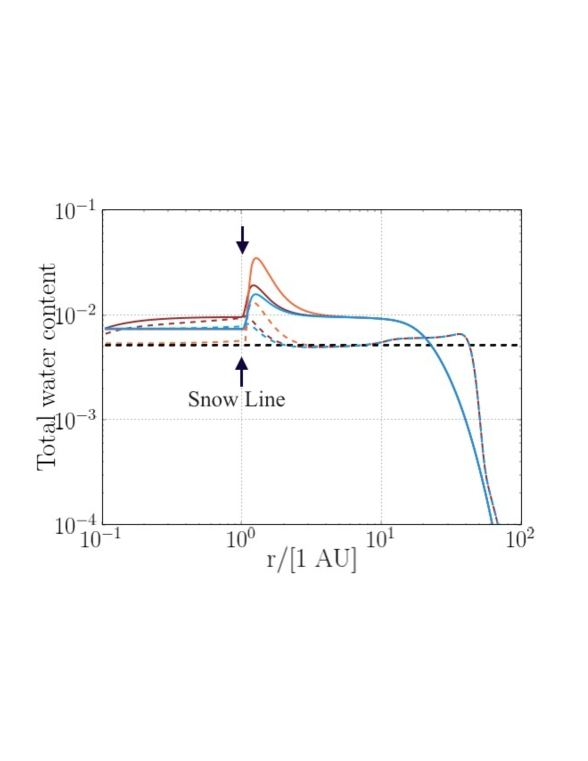
Figure 4: Simulated evolution over time of the total water abundance across disk radius $r$, i.e., ($\Sigma_{\rm vapor}+\Sigma_{\rm icychondrules}+\Sigma_{\rm icyasteroids}/\Sigma_{\rm gas}$) in a disk with accretional heating. Same as Figure 1: Blue profiles show 0.1 Myr (dashed) and 1 Myr (solid) with the formulation used here (cf. Gail 2001). Orange profiles similarly show formulations used by GH06/CC06, and brown profiles by SL88.

6 Summary

In the current literature, nine independent derivations have resulted in six mutually exclusive equations for volatile transport. These different treatments make significantly different predictions about the abundance of water and the surface density of ice. The large difference in predicted outcomes underscores how important it is to use the correct equation to calculate radial transport of volatiles. We have derived the volatile transport equations starting with Fick’s law and have identified the correct equations to use. With the discrepancies between existing treatments explained and the correct forms identified, we hope that this paper can serve as a resource for the disk modeling community.

References

- Birnstiel et al. (2010) Birnstiel, T., Dullemond, C. P., Brauer, F. 2010. Gas and dust evolution in protoplanetary disks. Astronomy and Astrophysics 513, A79.
- Bockelée-Morvan et al. (2002) Bockelée-Morvan, D., Gautier, D., Hersant, F., Huré, J.-M., Robert, F. 2002. Turbulent radial mixing in the solar nebula as the source of crystalline silicates in comets.. Astronomy and Astrophysics 384, 1107-1118.
- Brauer et al. (2008) Brauer, F., Dullemond, C. P., Henning, T. 2008. Coagulation, fragmentation and radial motion of solid particles in protoplanetary disks. Astronomy and Astrophysics 480, 859-877.
- Carballido et al. (2011) Carballido, A., Bai, X.-N., Cuzzi, J. N. 2011. Turbulent diffusion of large solids in a protoplanetary disc. Monthly Notices of the Royal Astronomical Society 415, 93-102.
- Ciesla (2009) Ciesla, F. J. 2009. Two-dimensional transport of solids in viscous protoplanetary disks. Icarus 200, 655-671.
- Ciesla and Cuzzi (2006) Ciesla, F. J., Cuzzi, J. N. 2006. The evolution of the water distribution in a viscous protoplanetary disk. Icarus 181, 178-204.
- Clarke and Pringle (1988) Clarke, C. J., Pringle, J. E. 1988. The diffusion of contaminant through an accretion disc. Monthly Notices of the Royal Astronomical Society 235, 365-373.
- Cuzzi and Weidenschilling (2006) Cuzzi, J. N., Weidenschilling, S. J. 2006. Particle-Gas Dynamics and Primary Accretion. Meteorites and the Early Solar System II 353-381.
- Cuzzi and Zahnle (2004) Cuzzi, J. N., Zahnle, K. J. 2004. Material Enhancement in Protoplanetary Nebulae by Particle Drift through Evaporation Fronts. The Astrophysical Journal 614, 490-496.
- Cuzzi et al. (1993) Cuzzi, J. N., Dobrovolskis, A. R., Champney, J. M. 1993. Particle-gas dynamics in the midplane of a protoplanetary nebula. Icarus 106, 102.
- Cuzzi et al. (2003) Cuzzi, J. N., Davis, S. S., Dobrovolskis, A. R. 2003. Blowing in the wind. II. Creation and redistribution of refractory inclusions in a turbulent protoplanetary nebula. Icarus 166, 385-402.
- Estrada et al. (2016) Estrada, P. R., Cuzzi, J. N., Morgan, D. A. 2016. Global Modeling of Nebulae with Particle Growth, Drift, and Evaporation Fronts. I. Methodology and Typical Results. The Astrophysical Journal 818, 200.
- Gail (2001) Gail, H.-P. 2001. Radial mixing in protoplanetary accretion disks. I. Stationary disc models with annealing and carbon combustion. Astronomy and Astrophysics 378, 192-213.
- Guillot and Hueso (2006) Guillot, T., Hueso, R. 2006. The composition of Jupiter: sign of a (relatively) late formation in a chemically evolved protosolar disc. Monthly Notices of the Royal Astronomical Society 367, L47-L51.
- Hartmann et al. (1998) Hartmann, L., Calvet, N., Gullbring, E., D’Alessio, P. 1998. Accretion and the Evolution of T Tauri Disks. The Astrophysical Journal 495, 385-400.
- Hirschfelder et al. (1964) Hirschfelder, J. O., Curtiss, C. F., & Bird, R. B. 1964. Molecular Theory of Gases and Liquids (Wiley, New York).
- Hughes and Armitage (2010) Hughes, A. L. H., Armitage, P. J. 2010. Particle Transport in Evolving Protoplanetary Disks: Implications for Results from Stardust. The Astrophysical Journal 719, 1633-1653.
- Johansen et al. (2007) Johansen, A., Oishi, J. S., Mac Low, M.-M., Klahr, H., Henning, T., Youdin, A. 2007. Rapid planetesimal formation in turbulent circumstellar disks. Nature 448, 1022-1025.
- Kalyaan et al. (2015) Kalyaan, A., Desch, S. J., Monga, N. 2015. External Photoevaporation of the Solar Nebula. II. Effects on Disk Structure and Evolution with Non-uniform Turbulent Viscosity due to the Magnetorotational Instability. The Astrophysical Journal 815, 112
- Kokubo & Ida (2002) Kokubo, E., & Ida, S. 2002. Formation of Protoplanet Systems and Diversity of Planetary Systems. The Astrophysical Journal 581, 666-680
- Launder (1976) Launder, B. E. 1976. Heat and mass transport. Turbulence. (A77-20355 07-34) Berlin and New York, Springer-Verlag, 1976, p. 231-287. 231-287.
- Lesniak & Desch (2011) Lesniak, M. V., & Desch, S. J. 2011, ApJ, 740, 118
- Lynden-Bell and Pringle (1974) Lynden-Bell, D., Pringle, J. E. 1974. The evolution of viscous discs and the origin of the nebular variables. Monthly Notices of the Royal Astronomical Society 168, 603-637.
- Lyons et al. (2009) Lyons, J. R., Bergin, E. A., Ciesla, F. J., Davis, A. M., Desch, S. J., Hashizume, K., Lee, J.-E. 2009. Timescales for the evolution of oxygen isotope compositions in the solar nebula. Geochimica et Cosmochimica Acta 73, 4998-5017.
- Marti & Mauersberger (1993) Marti, J., & Mauersberger, K. 1993. A Survey and New Measurements of Ice Vapor Pressure at Temperatures between 170 and 250K. Geophysical Research Letters 20, 363-366
- Mauersberger & Krankowsky (2003) Mauersberger, K., Krankowsky, D. 2003. Vapor pressure above ice at temperatures below 170K. Geophysical Research Letters 30, 1121 (21,1-3)
- McComb (1990) McComb, W. D. 1990. The physics of fluid turbulence. Chemical Physics .
- Morfill and Voelk (1984) Morfill, G. E., Voelk, H. J. 1984. Transport of dust and vapor and chemical fractionation in the early protosolar cloud. The Astrophysical Journal 287, 371-395.
- Nakagawa et al. (1986) Nakagawa, Y., Sekiya, M., Hayashi, C. 1986. Settling and growth of dust particles in a laminar phase of a low-mass solar nebula. Icarus 67, 375-390.
- Pasek et al. (2005) Pasek, M. A., Milsom, J. A., Ciesla, F. J., Lauretta, D. S., Sharp, C. M., Lunine, J. I. 2005. Sulfur chemistry with time-varying oxygen abundance during Solar System formation. Icarus 175, 1-14.
- Petaev et al. (2011) Petaev, M. I., Lehner, S. W., Buseck, P. R. 2011. Processing of Silicates in S-Rich Systems: Implications for the Origin of Enstatite Chondrites. Workshop on Formation of the First Solids in the Solar System 1639, 9095.
- Schräpler and Henning (2004) Schräpler, R., Henning, T. 2004. Dust Diffusion, Sedimentation, and Gravitational Instabilities in Protoplanetary Disks. The Astrophysical Journal 614, 960-978.
- Stepinski and Valageas (1996) Stepinski, T. F., Valageas, P. 1996. Global evolution of solid matter in turbulent protoplanetary disks. I. Aerodynamics of solid particles.. Astronomy and Astrophysics 309, 301-312.
- Stevenson and Lunine (1988) Stevenson, D. J., Lunine, J. I. 1988. Rapid formation of Jupiter by diffuse redistribution of water vapor in the solar nebula. Icarus 75, 146-155.
- Takeuchi and Lin (2002) Takeuchi, T., Lin, D. N. C. 2002. Radial Flow of Dust Particles in Accretion Disks. The Astrophysical Journal 581, 1344-1355.
- Voelk et al. (1980) Völk, H. J., Jones, F. C., Morfill, G. E., Roeser, S. 1980. Collisions between grains in a turbulent gas. Astronomy and Astrophysics 85, 316-325.
- Youdin and Lithwick (2007) Youdin, A. N., Lithwick, Y. 2007. Particle stirring in turbulent gas disks: Including orbital oscillations. Icarus 192, 588-604.
- Zolensky et al. (2006) Zolensky, M. E., and 74 colleagues 2006. Mineralogy and Petrology of Comet 81P/Wild 2 Nucleus Samples. Science 314, 1735.