Linear Additive Markov Processes

Abstract

We introduce LAMP: the Linear Additive Markov Process. Transitions in LAMP may be influenced by states visited in the distant history of the process, but unlike higher-order Markov processes, LAMP retains an efficient parameterization. LAMP also allows the specific dependence on history to be learned efficiently from data.

We characterize some theoretical properties of LAMP, including its steady-state and mixing time. We then give an algorithm based on alternating minimization to learn LAMP models from data.

Finally, we perform a series of real-world experiments to show that LAMP is more powerful than first-order Markov processes, and even holds its own against deep sequential models (LSTMs) with a negligible increase in parameter complexity.

1 Introduction

Markov processes [13] are arguably the most widely used and broadly known sequence modeling technique available. They are simple, elegant, and theoretically well understood. They have been extended in many directions, and form a useful building block for many more sophisticated approaches in machine learning and data mining. However, the Markovian assumption that transitions are independent of history given the current state is routinely violated in real-world data sequences, as the user’s full history provides powerful clues about the likely next state.

To address these longer-range dependencies, Markov processes have been extended from first-order models to $k$th-order models in which the next element depends on the previous $k$. Such models, however, have a parameter space that grows exponentially in $k$, so for large state spaces, even storing the most recent 5–6 elements of history may encounter data sparsity issues and impact generalization. Variable-order Markov processes [4] attempt to address these issues by retaining variable amounts of history, allocating more resources to remembering more important recent situations. Even here, a dependence on an element from the past can be used only if all intermediate sequences of states are remembered explicitly; there are exponentially many such sequences, and they may not impact the prediction in any way.

Beyond Markov processes, a wide range of more complex sequence models have been proposed. The last two decades have seen notable empirical success for models based on deep neural networks, particularly the Long Short-Term Memory (LSTM) architecture [12]. These LSTM models show state of the art performance in many domains, at the cost of low interpretability, long training times, and the requirement for significant parameter tuning.

Basic intuition. Our goal is to propose a model with the simplicity, parsimony, and interpretability of first-order Markov processes, but with ready access to possibly distant elements of history. The family of models we propose also has clean mathematical behavior, is easy to interpret, and comes equipped with an efficient learning algorithm.

The intuition behind our model is as follows. We select a sampled point from the user’s history, according to a learned time decay. We then assume that the user will adopt the same behavior as somebody in that prior context. Thus, if a recency-weighted sample of the user’s past shows significant time spent in the “parent” state and the “office worker” state, the model will offer next state predictions based on the current state, mixed with predictions that are appropriate for “parent” and “office worker.” The relative importance of the current state versus the historical norms will be learned from the data.

An overview of LAMP. Based on this intuition, we define a Linearly Additive Markov Process, or LAMP, based on a stochastic matrix $P$, and a distribution $w$ over positive integers. The matrix determines transitions from a given context, and the distribution captures how far back into history the process will look to select a context for the user. Given a user who has traversed a sequence of states $X=x_{1}x_{2}\ldots x_{t}$, the process first selects a past state $x_{i}$ with probability proportional to $w_{t-i+1}$, and then selects a next state $y$ using $P$ as a transition from $x_{i}$. Thus, the user chooses a next step by taking a step forward from some state chosen from the history. The matrix $P$ and the distribution $w$ are to be learned from data.

One may view LAMP as factoring the temporal effect from the contextual effect, resulting in a multiplicative model. When a state is chosen from the history, the behavior conditioned on that state is independent of how long ago the state was visited. This factoring keeps the model parsimonious.

We also consider a natural generalization of LAMP which we refer to as Generalized LAMP, or GLAMP. This extended model allows us to associate different matrices with different regions of history. For example, one matrix might capture transitions from the current state, taking into account geographic locality. Another matrix might capture transitions from past states, taking into account co-visitations. We define and characterize GLAMP.

Theoretical properties. LAMP is a generative sequence model related to Markov processes, but more expressive. It is therefore critical for us to understand the mathematical properties of the process, so we can evaluate whether LAMP is appropriate to model a particular dataset.

With this motivation in mind, we study the theoretical properties of LAMP. We show that LAMP models with $k$ elements of history cannot be approximated within any constant factor by Markov processes of order $k-1$, but can be captured completely by Markov processes of order $k$ (albeit with a parameterization that is exponentially larger in $k$). We show further that LAMP models under some mild regularity conditions do possess a limiting equilibrium distribution over states, and this distribution is equal to the steady state of the first-order Markov process defined by matrix $P$. However, beyond the steady state itself, the transition dynamics of the LAMP process are quite different from that of the Markov process on the same matrix, and are in general different from any first-order Markov Process. Finally, again under some mild conditions, we are able to characterize the convergence of LAMP to its steady state, in terms of properties of $P$ and $w$. In order to prove these results, we develop an alternate characterization of the process, dubbed the exponent process, which allows us to invoke the machinery of renewal processes in the analysis.

Learning and evaluation. Given data, the challenge for LAMP is to determine which stochastic matrix and distribution over positive integers will maximize likelihood of the observations. The learned matrix could in general be different from the empirical transition matrix, as the model might choose to “explain” certain transitions by reference to historical states rather than the current state.

To perform the learning, we show that the likelihood is convex in either $P$ or $w$ alone, and we give an alternating maximization procedure. We will discuss the optimization issues that arise in fitting this model accurately.

We then perform a series of experiments to evaluate the performance of LAMP. Our expectation is that LAMP will be useful in the same circumstances as Markov processes: as simple, interpretable, and extensible mathematical models, or as modules in larger statistical systems. We therefore begin by comparing LAMP to $k$th-order Markov processes, with and without smoothing. Of the four datasets we consider, our results show that for two of them, there is significant benefit to having the additional history provided by LAMP, and perplexity may be reduced by 20–40%. For the other two datasets we consider, the LAMP optimizer sets the weight distribution to place all mass on the most recent state, causing LAMP to fall back to a first-order Markov process. We therefore conclude that when benefits are attainable through long-distance dependencies, LAMP may show significant gains; otherwise, it degrades gracefully to a first-order Markov process. In this comparison LAMP and first-order Markov processes have similar parameter complexity: a large transition matrix in both cases, and optionally $k$ additional scalars for LAMP. To see any lift with such a modest additional parameterization is interesting. For completeness, we also compare LAMP with LSTMs. Our experiments show an intriguing outcome: neither LSTM nor LAMP is a clear winner on all datasets.

Overall, we find that LAMP represents an intriguing and valuable new point on the curve of accuracy versus complexity in finite-state sequence modeling.

2 Related Work

Markov processes have been studied for more than a century. The line of work most closely related to ours is that of Additive Markov processes, in which the Markovian assumption is relaxed to take some history into account. In particular, the probability of the next state is a sum of memory functions, where each function depends on the next state and the historical state. They were formally introduced as a probabilistic process by A. A. Markov [16], where versions of existing limit theorems for Markov processes were extended to this new framework. A first usage of these models to represent long range dependencies came in the context of physics and dynamical systems [29, 17, 28]. In all of these works, however, the state space is restricted to binary and the construction of the memory function is empirical.

Independent of our work and recently, Zhang et al. [35, 34] use a “gravity model”, which is similar to LAMP in that it is parameterized by a transition matrix and a history distribution. However, they make no attempt to learn the parameters in a robust manner. Instead, the transition matrix is estimated as the empirical transition matrix of a first-order Markov process from the data, and the history distribution is assumed to be from a particular family. We, in addition to providing a theoretical treatment of LAMP, also develop a principled method to learn the parameters without assumptions on the form of the history function.

There have been several lines of work that go beyond the Markovian assumption in order to capture user behavior in real-world settings. Higher-order and variable-order Markov processes [4, 25, 23] use the last few states in the history to determine the probability of transition to the next state. While they are strictly more powerful than the first-order Markov process, they suffer from two drawbacks. First, they are expensive to represent since the amount of space needed to store the transition matrix could be exponential in the order, and second, from a learning point of view they are particularly vulnerable to data sparsity. LAMP, on the other hand, is succinctly representable and has no data sparsity issues.

Motivated by web browsers, Fagin et al. [10] propose the ‘Back Button’ random walk in which users can revisit steps immediately prior in their history as the next state they transition to. However the back button model erases history when moving backwards, while LAMP retains it. Pemantle et al. [20] suggest a node-reinforced random walk, where popular nodes are re-visited with higher proportions. This is one method for utilizing user history while maintaining a small set of parameters. But the total number of visits to a node cannot be so easily adapted to take into account temporal relevance. LAMP, on the other hand, can easily incorporate recency via the history distribution. This notion of using summary statistics is also studied in Kumar et al. [15] in a different framework, with summary statistics used to infer facts about an underlying generative process, which is assumed to be Markovian.

Markov processes have been used in several web mining settings to model user behavior. PageRank [19] is a classic use of random walks to capture web surfing behavior. First and higher-order Markov processes have been used to model user browsing patterns [19, 24, 26, 36, 21] and variable-order Markov processes have been used to model session logs [2]. First-order Markov processes [1, 7] and variable-order hidden Markov processes [5] have often been applied to context-aware search, document re-ranking, and query suggestions. Chierichetti et al. [6] study the problem of using variable-order Markov processes to model user behavior in different online settings. Singer et al. [27] combine first-order Markov processes with Bayesian inference for comparing different prior beliefs about transitions between states and selecting the Dirichlet prior best supported by data. Our experiments suggest that LAMP can go well beyond first-order Markov processes, with negligible increase in space and learning complexities. We believe LAMP will be a powerful way to model user behavior for many of these applications.

3 LAMP

In this section we introduce the Linear Additive Markov Process (LAMP), and describe its properties.

3.1 Background

Let $[n]=\{1,2,\ldots,n\}$. Let ${\cal X}$ be a state space of size $n$. We use lower case $x,y,\ldots$ and its subscripted versions to denote elements of ${\cal X}$ and upper case $X,Y,\ldots$ and its subscripted versions to denote random variables defined on ${\cal X}$. Let $\{P(x,y)\}$ be an $n\times n$ stochastic matrix defined on ${\cal X}$, with $P(x,y)\geq 0$ and for all $x\in{\cal X}$, $\sum_{y\in{\cal X}}P(x,y)=1$.

The matrix $P$ naturally corresponds to a first-order Markov process on the state space ${\cal X}$ in which, given a current state $x$, the process jumps to state $y$ with probability $P(x,y)$. Formally, if $x_{0},\ldots,x_{t-1}$ are the states in the process so far, then

$$\Pr[X_{t}=x\mid x_{0},\ldots,x_{t-1}]=P(x_{t-1},x).$$ (1)

Let $P^{t}$ denote the matrix raised to the power $t$. Let $\mathrm{nnz}(P)$ denote the number of non-zero entries of $P$.

Let $\pi$ be the stationary distribution of $P$ satisfying

$$\sum_{x}P(x,y)\cdot\pi(x)=\pi(y),\mbox{ for all }y\in{\cal X}.$$

Equivalently, $\pi=\lim_{t\rightarrow\infty}\pi_{0}\cdot P^{t}$ for any starting distribution $\pi_{0}$. If $P$ is ergodic (see, e.g., [13] for formal definitions), then the stationary distribution $\pi$ of $P$ is well-defined and unique.

While the stationary distribution captures the asymptotic behavior of the Markov process, it does not quantify how fast it approaches this limit. The notion of mixing time captures this: it is the number of steps needed before the Markov process converges to its stationary distribution, regardless of the node from where it started. Formally, let $1_{z}$ denote the unit vector with $1$ in the $z$th position, and let

$$\Delta(P,t,z)=\frac{1}{2}\left|\pi-1_{z}\cdot P^{t}\right|=\frac{1}{2}\sum_{x}\left|\pi(x)-(1_{z}\cdot P^{t})(x)\right|,$$

denote the total variation distance between the stationary distribution and the distribution after $t$ steps when the Markov process starts at $z$. The mixing time, with respect to a parameter $\delta>0$, is then defined as:

$$t_{\mathrm{mix}}(P,\delta)=\max_{z}\left\{\min_{t}\left\{\Delta(P,t^{\prime},z)\leq\delta,\mbox{ for all }t^{\prime}\geq t\right\}\right\}.$$

A $k$th-order Markov process, $\mathsf{MC}_{k}$, for $k>1$, is defined as follows: let $P_{k}:{\cal X}^{k}\times{\cal X}\rightarrow\mathbb{R}$ be a stochastic matrix on ${\cal X}^{k}$, the space of $k$-tuples on ${\cal X}$. Then,

$$\Pr[X_{t}=x_{t}\mid x_{0},\ldots,x_{t-1}]=P(\left\langle x_{t-k},\ldots,x_{t-1}\right\rangle,x_{t}).$$ (2)

where $t>k$; we assume there is a starting distribution on tuples of length $k-1$.

Let $k$ be a non-negative integer. Let $w=(w_{1},\ldots,w_{k})$ be a distribution on $[k]$. The notation $W\sim w$ indicates that the random variable $W$ is chosen according to $w$, i.e., $\Pr[W=i]=w_{i}$.

3.2 Process definition

LAMP is parameterized by a matrix $P$ and a distribution $w$ on $[k]$. The process evolves similarly to a Markov process, except that at time $t$, the next state is chosen by drawing an integer $i$ according to $w$, and picking an appropriate transition from the state $i$ timesteps ago (or from the start state if $t-i<1$). Formally, we define it as follows.

Definition 1 (LAMP)

Given a stochastic matrix $P$ and a distribution $w$ on $[k]$, the $k$th-order linearly additive Markov process $\mathsf{lamp}_{k}(w,P)$ evolves according to the following rule:

$$\Pr[X_{t}=x_{t}\mid x_{0},\ldots,x_{t-1}]=\sum_{i=1}^{k}w_{i}\cdot P(x_{\max\{0,t-i\}},x_{t}).$$ (3)

When $k$ is implicit, we simply denote the process as $\mathsf{lamp}(w,P)$. We assume that the process starts in some state $\pi_{0}$. (As discussed later, the particular choice of starting state is unimportant.)

3.3 Key features

(i) LAMP is a superset of first-order Markov processes; just set $w_{1}=1$. We will show (Lemma 2) below that this is a strict containment, i.e., there are processes expressible with LAMP but provably not so with a first-order Markov process (despite the comparable number of parameters). We also explore other expressivity relations between Markov processes and LAMP (Section 3.4).

(ii) By controlling the distribution $w$, one can encode highly contextual transition behavior and long-range dependencies. The definition of $w$ determines how fast past history is “forgotten”, and allows a smooth transition from treating the recent past as a sequence, to treating the more distant past as a set, simply by flattening $w$.

(iii) While LAMP is a generative sequence model that allows long-range dependencies, the model complexity is only $\mathrm{nnz}(P)+k$. In contrast, the complexity of a $k$th-order Markov process is $\mathrm{nnz}(P_{k})$, which can be exponential in $k$. In natural extensions of LAMP, the distribution $w$ may be restricted to a family of distributions specified only by a constant number of shape parameters (e.g., power law, double Pareto, or log normal distributions).

(iv) An alternative characterization of LAMP provides a tractable and interpretable way to understand its behavior (Section 4).

(v) The LAMP model is easy to learn from data (Section 5). While LAMP is by construction intended to be a learned model with a tractable algorithm for the learning, the mathematical structure of the model belongs to a much larger and generally non-learnable Additive Markov processes (Section 7).

3.4 Expressivity

A natural starting point to understand LAMP is to compare it in terms of expressivity and approximability with Markov processes. We begin by asking how closely LAMP, which employs a stochastic matrix $P$, may be approximated by a first-order Markov process.

Lemma 2

There is a second-order LAMP that cannot be expressed by any first-order Markov process.

Proof 3.1.

Define $\mathsf{lamp}(w,P)$ as follows. The transition matrix $P$ consists of a cycle on ${\cal X}=[n]$, with $P(i,i+1)=1$ for $i\neq 1$, and $P(1,1)=\epsilon,P(1,2)=1-\epsilon$ for some small $\epsilon>0$ (this is to ensure mixing). Let $k=2$ and $w=(1/2,1/2)$. All the additions are modulo $n$.

By the definition of $w$ and (3), we can see that a sequence generated by $\mathsf{lamp}(w,P)$ can contain the pattern $\ldots,i-1,i,i,\ldots$ but can never contain the pattern $\ldots,i,i,i,\ldots$. I.e., $\mathsf{lamp}(w,P)$ can produce two repeats of a state but not three. However, if we try to represent this process with a first-order Markov process $P_{1}$, then consider $P_{1}(i,i)$. If $P_{1}(i,i)=0$, then the first-order process can never generate the first pattern and if $P_{1}(i,i)>0$, then the first-order process generates the second pattern with positive probability. Neither of them is correct compared to $\mathsf{lamp}(w,P)$.

This example can be easily extended to show that there is a $k$th-order LAMP that cannot be well approximated by any $(k-1)$st-order Markov process. In summary, though the additional parameters of a $\mathsf{lamp}(w,P)$ are few, they are sufficient to give LAMP more degrees of expressivity.

Of course, if the order of the Markov process is high enough, then it strictly contains all LAMPs of a particular order. The following statements make this precise.

Lemma 3.2.

$k$th-order LAMPs can be expressed by $k$th-order Markov processes.

Proof 3.3.

From (3), that the transitions of $\mathsf{lamp}_{k}(w,P)$ depend only on $k$ tuples, since $w$ has a support of size $k$. Therefore, one can trivially use a $k$th-order Markov process to (wastefully) represent the transition probabilities.

Lemma 3.4.

For $k\geq 2$, there is a $k$th-order Markov process that is not expressible by a $k$th-order LAMP.

Proof 3.5.

For sake of simplicity, we present the proof for $k=2$; the general case can be proved using similar ideas.

We consider a second-order Markov process on two states, ${\cal X}=\{x,y\}$. We explicitly construct the following $P_{2}$ that is not expressible as a second-order LAMP. Let $\beta\neq\gamma$ and $\alpha=1-\delta$.

$P_{2}$ $x$ $y$ $\left\langle x,x\right\rangle$ $\alpha$ $1-\alpha$ $\left\langle x,y\right\rangle$ $\beta$ $1-\beta$ $\left\langle y,x\right\rangle$ $\gamma$ $1-\gamma$ $\left\langle y,y\right\rangle$ $\delta$ $1-\delta$

Suppose $P_{2}$ is expressible by $\mathsf{lamp}_{2}(w,P)$ for some $w$ on $[2]$ and some stochastic matrix $P$. We first claim that $P(x,x)=\alpha$ and $P(y,y)=\delta$, i.e., the diagonals are fixed. This follows from the definition of $P_{2}$ and (3) since, for example,

$$\alpha=P_{2}(\left\langle x,x\right\rangle,x)=\Pr[x\mid\left\langle x,x\right\rangle]=\sum_{i=1}^{2}w_{i}P(x,x)=P(x,x).$$

For the non-diagonals, we can compute

$$\beta=P_{2}(\left\langle x,y\right\rangle,x)=w_{1}\alpha+(1-w_{1})(1-\delta),$$

$$\gamma=P_{2}(\left\langle y,x\right\rangle,x)=w_{1}(1-\delta)+(1-w_{1})\alpha.$$

It is easy to check that the above system is inconsistent with the imposed conditions $\beta\neq\gamma$ and $\alpha=1-\delta$.

Note that this result that $\mathsf{lamp}_{k}\ \lower 2.15277pt\hbox{$\stackrel{{\scriptstyle\subset}}{{\small{\tiny\mbox{$\neq$}}}}$}\ \mathsf{MC}_{k}$ is also intuitive, as a $k$th-order Markov Process has $O(n^{k})$ parameters, compared to a $k$th-order LAMP, which only has $n^{2}+k$ parameters. The surprising aspect is that incorporating a little more trail history with just a few more parameters leads to inapproximability by lower order Markov processes, i.e., $\mathsf{lamp}_{k}\not\subseteq\mathsf{MC}_{k-1}$.

4 Analysis of LAMP

Despite the differences in expressivity of LAMP and Markov processes, we show that under fairly general conditions they share the same limiting distribution over states, although the limiting distribution on paths of length more than 1 may be very different.

As LAMP’s evolution depends on history, we cannot simply characterize its limiting distribution as a fixed point distribution on the graph. Instead, we say that $\mathsf{lamp}(w,P)$ has a limiting distribution $\pi$ if $\pi$ is a probability distribution over all states and $\pi(x)$ is the probability of finding the LAMP at state $x\in{\cal X}$ in the limit. Next, we study the mixing time of $\mathsf{lamp}(w,P)$ and relate it to the mixing time of $P$ and the properties of $w$. Mixing time for LAMP is defined analogously to Markov processes; we denote this by $t_{\mathrm{mix}}(\mathsf{lamp}(w,P),\delta)$. This study also leads us to a connection between the evolution of $\mathsf{lamp}(w,P)$ and the theory of stochastic processes, particularly martingales and renewal theory. This enables us to invoke results from these areas, and precisely describe the long-term behavior of LAMP. Besides being of theoretical interest, knowing the mixing time of LAMP is important to make conclusions about the validity of the learned model on real data. In particular, we study the conditions under which mixing time of LAMP can significantly depart from that of a Markov process.

4.1 Exponent process

To shed light on $\mathsf{lamp}(w,P)$, we present a re-characterization of the process in terms of certain exponents and mixtures of powers of $P$. Suppose $\pi_{0}$ is an initial distribution on ${\cal X}$ and suppose we run $\mathsf{lamp}_{2}(w,P)$. After the first step, the state distribution is given by $\pi_{0}P$. After the second step, with probability $w_{1}$ we have the distribution $\pi_{0}P^{2}$ and with probability $1-w_{1}$ we moved forward from $\pi_{0}$ again, and have the distribution $\pi_{0}P$. After the third step, with probability $w_{1}w_{2}$ we have the distribution $\pi_{0}P^{3}$, with probability $(1-w_{1})w_{2}+w_{1}(1-w_{2})$ we have the distribution $\pi_{0}P^{2}$, and so on. In this interpretation, the distribution of a Markov process after $t$ steps will be as $\pi_{0}P^{t}$, while the distribution of LAMP will be the expectation of a random variable $\pi_{0}P^{e_{t}}$, where $e_{t}$ depends on the random choices made from the history distribution, and may grow and shrink over time. We focus on the evolution of this exponent.

More formally, let $e_{t}$ be the random variable denoting the exponent at time $t$. The next state of the process is determined by choosing an earlier state $t-i$ according to $w$, itself distributed as $\pi_{0}P^{e_{t-i}}$, and then advancing one step from this state. Once the choice has been made to copy from $i$ states earlier, The new exponent will therefore be $e_{t}=1+e_{t-i}$. From this intuition, we define the following stochastic process, which we use to analyze size of the exponents.

Definition 3 (Exponent process).

Let $W_{1},W_{2},\ldots$ be i.i.d. random variables where $W_{t}\sim w$. For $t\in\mathbb{Z}$, the exponent process is the sequence of random variables $e_{t}$, with $e_{t}=0$ for $t\leq 0$, $e_{1}=1$, and for $t>1$:

$$\Pr[e_{t}=e_{t-i}+1]=\Pr[W_{t}=i].$$

Note that for a first-order Markov process, the exponent process is deterministic and is simply $...,0,1,2,\ldots$. For LAMP, the exponent process is more complex. In the following sections, we explore this process further, and discover not only concrete statements about the limiting behavior and convergence to equilibrium, but also connections to the theory of renewal processes. As $e_{t}$ is pre-defined for $t\leq 0$, from henceforth we assume $t\geq 0$.

We begin with a simple observation on the growth rate.

Lemma 4.6.

$e_{t}\geq\lfloor t/k\rfloor$.

Proof 4.7.

We can break the exponent process into consecutive batches of length $k$, where batch $B_{i}=\{e_{ik+1},\ldots,e_{(i+1)k}\}$. Then $\min\{B_{i}\}\geq 1+\min\{B_{i-1}\}$, since $e_{t}=1+e_{j}$ for some $j$ in $\{t-k,\ldots,t-1\}$. Thus, the minimum exponent must grow by 1 every $k$ steps.

This immediately gives the limiting distribution of LAMP:

Theorem 4.

$\mathsf{lamp}(w,P)$ has a limiting distribution $\pi$ if and only if $P$ is ergodic. Furthermore, $\pi$ is also the stationary distribution for the first-order Markov process with transition matrix $P$.

Proof 4.8.

The distribution of LAMP is given by the product of the start state with a mixture of powers of the transition matrix $P$ of the underlying Markov process. Lemma 4.6 gives a lower bound on every exponent in the mixture, and this lower bound increases without bound.

Note that the proof above only addresses the finite $k$ case. A similar result can be stated, with probability almost surely, for the infinite $k$ case, using results similar to Section 4.2. Theorem 4 also has a direct proof, which can be used to show a similar limiting distribution result for a generalization of LAMP (details omitted).

Next, we study the mixing time of LAMP in more detail. Lemma 4.6 gives us a bound on the mixing time, but this bound characterizes the worst case. We now seek a stronger bound based on the average case evolution of the exponent process.

4.2 Analysis with renewal theory

Consider the exponent process at a particular time $t$, with exponent $e_{t}$. We may trace the origins of this exponent backwards through the evolution of the process. At time $t$, the process chose a point $t-i$ from $i$ steps in the past, and added 1 to the exponent at that time. Similarly, at time $t-i$, the process chose another point even farther in the past from which to step forward. This backward chaining process is depicted in Figure 1. The number of hops traversed backward at each step is selected i.i.d. from $w$. For any point $t$, we may therefore define a sequence of decreasing positions $t=t_{0}>t_{1}>\cdots>t_{H(t)}$, with

$$e_{t_{i}}=e_{t_{i+1}}+1,$$

and $H(t)$ a stopping time, with $t_{H(t)}$ the first term $\leq 0$. The total number of hops in this evolution is exactly $H(t)=e_{t}$, as each step increases the exponent by 1.

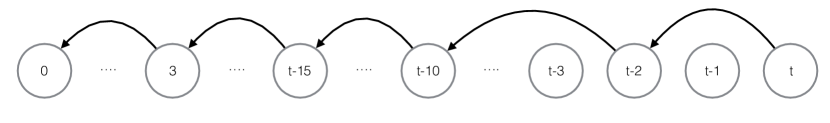
Figure 1: Recovering backward chain from time $t$: $t_{0}=t,t_{1}=t-2,t_{2}=t-10,\ldots,t_{5}=0$. Here, $H(t)=5$.

We now recall the definition of a renewal process, and show that the process defined above is a renewal process:

Definition 5 (Renewal process).

Let $S_{1},S_{2},\ldots$ be a set of positive i.i.d. random variables, and for $n\in\mathbb{Z}^{+}$ define the $n$th jump time $J_{n}=\sum_{i=1}^{n}S_{i}$. Then the random variable $(X_{t})_{t\geq 0}$ defined by $X_{t}=\sup\{n~{}\mid~{}J_{n}\leq t\}$ is called a renewal process.

The connection to LAMP is made explicit as follows:

(i) The gaps $t_{i}-t_{i+1}$, each drawn i.i.d. from $w$, correspond to the holding time variables $S_{i}$.

(ii) $H(t)$ correspond to the random variables $X_{t}$ forming the renewal process.

Based on this connection, we can employ the strong law of large numbers for renewal processes [22] to show the following theorem:

Theorem 6.

$$\lim_{t\rightarrow\infty}\frac{H(t)}{t}=\frac{1}{E[w]},\hskip 14.22636pt\mbox{almost surely}.$$

Note that this bound is much stronger than the bound of Lemma 4.6. Based on this bound, we see that the mixing time of LAMP is related to the mixing time of the underlying Markov process by a multiplicative factor of $E[w]$ as long as the renewal process has attained its limiting behavior.

One can then refer to the well-known central limit Theorem [22] for renewal processes to get concentration bounds.

Theorem 7.

If $W$ has finite mean and variance $\mu$ and $\sigma$, then

$$\lim_{t\rightarrow\infty}\Pr\left[\frac{H(t)-t/\mu}{\sigma\mu^{-3/2}\sqrt{t}}<\alpha\right]=\phi(\alpha),$$

where $\phi$ is the cdf of the standard Gaussian distribution.

However, with slightly stronger assumptions on the moments of $W$, we can also obtain growth rates for finite $t$.

4.3 Concrete growth rates and mixing time

To address our original question on mixing times, we derive the following concrete growth rate via Bernstein’s inequality [8].

Theorem 8.

For $k$ finite, for all $t\geq T$,

$$\Pr\left[e_{t}\geq\frac{t}{(1+\epsilon)E[w]}\right]\geq 1-\frac{e^{-C(\epsilon)\cdot T}}{1-e^{-C(\epsilon)}},$$

where $C(\epsilon)$ is a constant depending on $\epsilon,k$, and some of the moments of $w$.

this version.) This immediately bounds the mixing time.

Theorem 9.

For $w$ with finite support $[k]$, we have

$$t_{\mathrm{mix}}(\mathsf{lamp}(w,P),\delta)\leq\max\left\{T,(1+\epsilon)E[w]\cdot t_{\mathrm{mix}}(P,\delta)\right\},$$

with probability at least $1-\frac{e^{-C(\epsilon)\cdot T}}{1-e^{-C(\epsilon)}}$.

We can also establish similar results (formal statement and proofs omitted in this version) for infinite $k$ using the following:

Theorem 10.

Let $E[|w|^{4}]\leq\infty$. Then, for all $t\geq T$,

$$\Pr\left[e_{t}\geq\frac{t}{(1+\epsilon)E[w]}\right]\geq 1-O\left(\frac{1}{T}\right).$$

With these results, we conclusively establish long-term behavior of $\mathsf{lamp}(w,P)$, and next look at learning the model.

5 Learning the parameters

We now show how to learn the parameters of LAMP, given a sequence of observations. The input to the learning problem is a sequence $x_{0},\ldots,x_{t}$ of states, on a state space ${\cal X}$. The goal is to learn the transition matrix $P$ and the distribution $w$ that maximizes the likelihood of the observed data.

Given the sequence of states, by the definition of LAMP, we have

$$\Pr[x_{k+1}\mid x_{1},\ldots,x_{k}]=\sum_{i=1}^{k}w_{i}\cdot P(x_{k+1-i},x_{k+1}).$$

In particular, the likelihood function decomposes into a product of such terms and so the log likelihood is

$$L(x_{0},...,x_{t})=\sum_{j=0}^{t}\log\left(\sum_{i=1}^{k}w_{i}\cdot P(x_{j-i},x_{j})\right).$$

From here onwards we write $x_{0}$ in place of $x_{\max\{0,l\}}$ to simplify the notation.

To compute the gradient with respect to the entries of the transition matrix $P$, we compute the gradient with respect to each term in the above expression and put it together. Let $I(\cdot)$ denote the binary indicator function. We first have

$$\frac{\partial L}{\partial P(x,y)}=\sum_{x_{j}=y}\displaystyle{\frac{\sum_{i=1}^{k}I(x_{j-i}=x)\cdot w_{i}}{\sum_{i^{\prime}=1}^{k}w_{i^{\prime}}P(x_{j-i^{\prime}},x_{j})}}.$$

For the entries of $w$, we have

$$\frac{\partial L}{\partial w_{i}}=\sum_{j=0}^{t}\frac{P(x_{j-i},x_{j})}{\sum_{i^{\prime}=1}^{k}w_{i^{\prime}}P(x_{j-i^{\prime}},x_{j})}.$$

It is easy to show that the log likelihood is individually concave in $P(\cdot,\cdot)$ and $w$ but not jointly concave (proofs omitted). We run an alternating minimization to optimize for $P$ and $w$ holding the other parameters fixed. Recall that $w$ and every row of $P$ is non-negative and sums to $1$. Because of the latter constraint, generic unconstrained or box-constrained optimization algorithms such as L-BFGS(-B) cannot be applied to our problem directly.

Let us consider optimizing $w$ while holding $P$ fixed first. By the Karush–Kuhn–Tucker (KKT) optimality conditions we have that $w^{*}$ is optimum if and only if there exist $\lambda>0$, Lagrange-multiplier, such that $\frac{\partial L}{\partial w_{i}}(w^{*})=\lambda$ if $w_{i}^{*}>0$ and $\frac{\partial L}{\partial w_{i}}(w^{*})\leq\lambda$ if $w_{i}^{*}=0$. Generally, similar KKT conditions can be solved with complicated sequential quadratic programming or with interior-point methods [18]. Instead, we recognize that our KKT condition is a non-trivial extension of the water-filling problem [3, Example 5.2], that arises in information theory in allocating power to a set of communication channels. Starting from $\lambda=\infty$, attained by setting all $w_{i}^{*}=0$, we swipe with $\lambda$ towards $0$ until we find a $\lambda$ value satisfying the KKT conditions with corresponding $w^{*}$ that sums to one. To compute changes in $\frac{\partial L}{\partial w_{i}}$ we rely on the Hessian of $L$, i.e., we apply Newton’s method. Furthermore, we pretend that $H$ is diagonal. While this assumption is clearly false for $w$, the approximation is good enough that the resulting method works well in practice.

Then given an initial guess, $w^{0}$, our goal is to find an adjustment $u$ such that $w^{0}+u$ is still feasible, i.e., $\sum_{i}u_{i}=0$ and $0\leq w^{0}_{i}+u_{i}$ hold for all $i=1,\ldots,k$, and the KKT condition is satisfied by $w^{0}+u$. Such $u$ can be found with the aforementioned water-filling technique relying on the fact that each approximate $\frac{\partial L}{\partial w_{i}}$ becomes a linear function. We iteratively apply these adjustments until the KKT condition is satisfied up to a small error. Since our Hessian approximation introduces errors, it can happen that an adjustment would decrease the log likelihood. To combat this issue, we apply the well-known trust region method [18] and search for an adjustment $u$ with $\max_{i}{|u_{i}|}\leq r_{t}$, where $r_{t}$ is the size of the trust region in the $t$th adjustment step. Note that optimizing over $P$ decomposes over optimizing rows of $P(x,\cdot)$, where optimizing each row $P(x,\cdot)$ is analogous to optimizing $w$. Furthermore it is not hard to see that the Hessian is indeed diagonal in this case. Thus we optimize each row of $P(x,\cdot)$ while holding the rest fixed, i.e., we perform block coordinate descent.

Lastly we remark that Duchi et al.’s projected gradient method [9] is also applicable to our problem. We found it slow to converge as all gradients are equal and positive in optimum typically.

6 Experiments

In this section we present our experimental results on LAMP. The goal of these experiments is to model real-world sequences with LAMP and compare their performance with first- and higher-order Markov processes. For comparing the performance, we focus on standard notions such as perplexity. En route we also evaluate the performance of the learning algorithm based on alternative minimization, focusing on the number of iterations, convergence, etc. First we describe the datasets used for evaluation.

6.1 Data

We use the following datasets. Each dataset is a sequence of items over a particular domain. Since we are interested in modeling the transitions, the items will correspond to the states in LAMP (and in the Markov processes we will compare against) and we will not use any metadata about the items themselves. For repeatability purposes, we only focus on publicly available data.

Lastfm. This data is derived from the listening habits of users on the music streaming service last.fm [11]. In this service, users can select individual songs or listen to stations based on a genre or artist. We will focus on sequences, where each sequence corresponds to a user and each item in the sequence is the artist for the song (we focus on artists instead of individual songs). The data consists of 992 sequences with 19M items. The data is available at dtic.upf.edu/~ocelma/MusicRecommendationDataset/lastfm-1K.html.

BrightKite. BrightKite is a defunct location-based social networking website (brightkite.com) where users could publicly check-in to various locations. Each sequence corresponds to a user and each item in the sequence is the check-in location (i.e., the geographical coordinates) of the user. The data consists of 50K sequences with 4.7M check-ins. This dataset is available at snap.stanford.edu/data/loc-brightkite.html.

WikiSpeedia. This dataset is a set of navigation paths through Wikipedia, collected as part of a human computation game [31, 32]. In the game users were asked to navigate from a starting Wikipedia page to a particular target only by following document links. The dataset consists of 50K (source, destination) paths, which will form the sequences for our experiments; the items in a sequence will correspond to the Wikipedia pages. The dataset is available at snap.stanford.edu/data/wikispeedia.html.

Reuters. As an illustration of the performance of LAMP on a text dataset, we consider the Reuters-21578, Distribution 1.0 benchmark corpus (available at www.nltk.org/nltk_data/) as a baseline. Here, each newswire article is considered to be a single sequence and the items are the words in the sequence. The data consists of more than 1.2M words.

To mitigate data issues, we focus on non-consecutive reasonably frequent visits. Since consecutive repetitions for Lastfm might mean songs from the same CD and for BrightKite might mean being in the same place—yielding easy to learn, mundane first-order models with dominant self-loops as best fit,—we collapse consecutive repeated items into a single item. We then replace items that appear fewer than 10 times (in the original sequence) by a generic ‘rare’ item; this threshold is 50 for Lastfm.

6.2 Baselines

We compare LAMP to various baselines, defined as follows.

Naive $N$-gram. An order-$k$ Naive $N$-gram behaves as $\mathsf{MC}_{k}$, i.e., a $k$th-order Markov process, which employs counts of the previous $k$ elements to predict the next element. Since a second-order Markov process in fact uses statistics about 2 past and 1 future element, order-2 corresponds to 3-grams, and generally, order-$k$ corresponds to $k+1$-grams. We retain the notion of order so that order-1 Naive $N$-gram will be equivalent to order-1 LAMP.

Kneyser–Ney $N$-gram. This baseline employs state-of-the-art smoothing of $N$-grams using the Kneyser–Ney algorithm [14]. It corresponds to a variable-order Markov process, in that it employs as much as context as possible, given the available data, falling back to lower-order statistics as necessary.

LSTM. This baseline trains an LSTM (Long Short Term Memory) architecture on the datasets. The LSTM is a type of recurrent neural network [12], which has recently been very successful in modeling sequential data.

Weight-only LAMP. This baseline corresponds to running the LAMP algorithm with the matrix $P$ fixed to the empirical transition matrix, learning only the weights $w$.

Initial weights. This baseline corresponds to LAMP with the matrix $P$ fixed to the empirical transition matrix and the history distribution defined as $w_{i}\propto 0.8^{i}$. We always initialized the alternating minimization to these values and hence this baseline.

6.3 Results

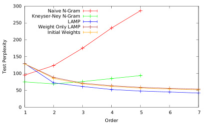
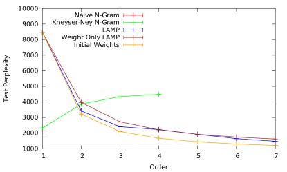
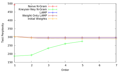
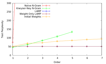
Figure 2: Order vs test perplexity for LAMP, weight-only LAMP, MLE and Kneyser–Ney N-grams. Top left: BrightKite, top right: Lastfm, bottom left: Reuters, bottom right: WikiSpeedia.

We compare LAMP to the $N$-gram variants and to the LSTM.

6.3.1 LAMP and $N$-grams

Perplexity. Figure 2 gives our main results on the perplexity of various order models, across our datasets. The first chart of the figure covers BrightKite data, and shows that all LAMP variants outperform the Markov models on test perplexity, with an order-7 LAMP showing around 19% improvements over the simpler variants at the same order.

For Lastfm, again LAMP variants outperform N-grams, producing text perplexity around 50% lower than smoothed N-grams, and far lower than naive N-grams, which overfit badly. In this case, among the LAMP variants, the exponential weights improve over the optimized by about 18% at order 7. The optimized weights perform better than exponential on training perplexity, so the algorithm could benefit from some additional regularization.

For Reuters, LAMP models perform similarly to one another, and the naive N-grams perform so poorly that they do not register on the chart. The smoothed N-grams outperform all LAMP variants. However, despite the smoothing, their performance on test worsens as the data becomes too sparse; this is a regime where the smoothing is not designed to operate. For this data, LAMP sets $w_{1}=1$, behaving as a first-order Markov process, and higher-order N-grams are able to perform better, albeit with the usual trade-off of higher numbers of parameters.

Finally, for WikiSpeedia, naive and smoothed N-grams perform substantially worse than LAMP variants, with LAMP and weight-only LAMP performing best.

As described in Lemma 3.2, $\mathsf{MC}_{k}$ is more expressive than $\mathsf{lamp}_{k}$, so one may wonder how it is possible that order-$k$ LAMP may show better performance than a $k$th-order Markov process. In fact, the Markov process performs significantly better in training perplexity, but despite our tuning of the Kneser–Ney smoothing, LAMP generalizes better.

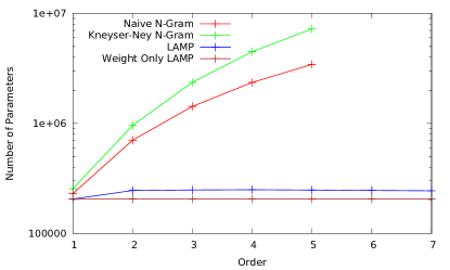
Figure 3: Order vs number of parameters for BrightKite. Other datasets are similar.

Number of parameters. Figure 3 shows how the actual number of parameters changes with order for the various models. For the LAMP models, the number of parameters could theoretically grow as order increases, because the optimizer will see possible transitions from earlier states, and might choose to increase the density of the learned matrix. For example, on an expander graph, a sparse transition matrix could even grow exponentially in density as a function of order until the matrix becomes dense. While this growth is possible in theory, it does not occur in practice. The BrightKite dataset shows a small increase in parameters from first to second order LAMP, and the remaining datasets show no significant increase in parameters whatsoever. The N-gram algorithms show in all cases a dramatic increase in parameters, to the extent that we could run these baselines only to order 5 (and order 3 for Lastfm).

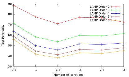
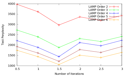
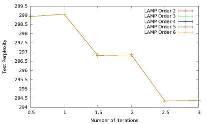
Figure 4: Number of iterations in alternating minimization vs test perplexity for LAMPs of various order. $i-0.5$ is the $i$th weigh optimization, $i$ is the $i$th transition matrix optimization. Top left: BrightKite, top right: Lastfm, bottom left: Reuters, bottom right: WikiSpeedia, error bars show standard deviation in $10$-fold cross validation; repeated for 2 datasets.

Number of rounds. Figure 4 shows how the performance of LAMP changes over the rounds of optimization. For BrightKite and Lastfm, the algorithm performs best at 1.5 rounds, meaning the weights are optimized, then the matrix, and then the weights are re-optimized for the new matrix. For Reuters, small improvements continue beyond this point, and performance for WikiSpeedia is flat across iterations. The appropriate stopping point can be determined from a small holdout set, but from our experiments, performing 1.5 rounds of optimizations seems effective.

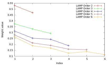
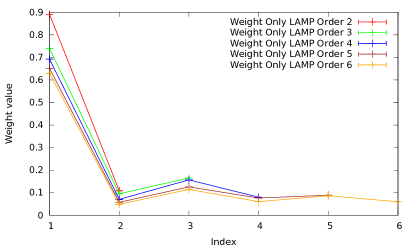
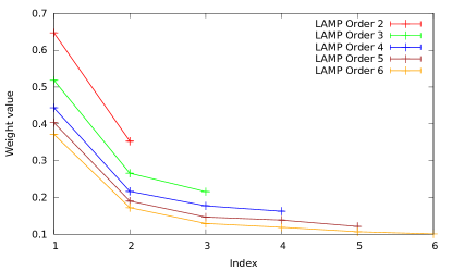
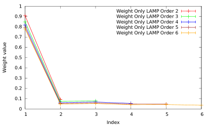
Figure 5: Estimated weight values for LAMPs of various order (left) and weight-only LAMPs (right), Top left: BrightKite, top right: Lastfm, bottom left: Reuters, and bottom right: WikiSpeedia set $w_{1}=1$.

Learned weights. We now turn to the weight values learned by the LAMP model; see Figure 5. BrightKite and Lastfm show a similar pattern: when the matrix is fixed to the empirical observed transitions (right column), the weights decay rapidly, putting most of their focus on the most recent state. This behavior is expected, as the matrix in this case has been selected to favor the most recent state. However, when LAMP is given control of the matrix, the optimizer selects a matrix for which a flatter weight distribution improves likelihood, making better use of history.

We also observe that the relative values of earlier weights in lower-order versus higher-order LAMP are similar. As order increases, all the weights are dropped slightly to allow some probability mass to be moved to higher weights corresponding to influence from more distant information.

Both Reuters and WikiSpeedia assign $w_{1}=1$, indicating that LAMP’s history is not beneficial in modeling these datasets.

6.3.2 LAMP and LSTM

To this point, we have considered LAMP as an alternative sequence modeling technique to Markov processes, appropriate for use in similar situations. In this section, we consider the performance of LAMP relative to LSTMs, which lie on the alternate end of the spectrum: they are highly expressive recurrent neural networks representing the best of breed predictor in multiple domains, with an enormous parameter space, high training latency, low interpretability, and some sensitivity to the specifics of the training regime. We use a slight variant of the ‘medium’-sized LSTM [33]. We perform comparisons for Lastfm, BrightKite, and Reuters; the WikiSpeedia dataset is too small to showcase the strengths of LSTMs, so we omit it. Table 1 shows the results.

Algorithm	BrightKite	Lastfm	Reuters
LAMP order 6, 1.5 iter	$38.4$	$1054.6$	$296.8$
LSTM, short training time	$85.8$	$1359.1$	$105.4$
LSTM, long training time	$51.0$	$525.7$	$60.4$

Table 1: Perplexity of LAMP and LSTM. Short training time for LSTM is same as LAMP; long training time is $20$x LAMP.

LAMP performs well on BrightKite relative to the LSTM. Even after 20x training time the LSTM’s perplexity is about 1/3 higher than LAMP, at which point the LSTM begins to overfit.

On Lastfm, the LSTM with similar training time to LAMP performs about 30% worse, but with additional training time, the LSTM performs significantly better, attaining about 50% of the test perplexity of LAMP, reducing from about 10 bits to about 9 bits of uncertainty in the prediction. We hypothesize this is because of additional structure within the music domain.

LSTMs are known to perform well on language data as in the Reuters corpus, and pure sequential modeling is unlikely to capture the nuance of language in the same way. The results are consistent with this expectation: LSTM with short training time already attains around $1/3$ the test perplexity of LAMP, and with more training, the LSTM improves to roughly $1/5$ of LAMP.

In summary, we expect that in general, LSTMs will outperform simpler techniques for complex sequential tasks such as modeling language, speech, etc. We expect that LAMPs will be more appropriate in settings in which Markov processes are typically used today: as simple, interpretable, extensible sequence modeling techniques that may easily be incorporated into more complex systems. Nonetheless, it is interesting that for datasets like BrightKite and Lastfm, LAMP performs on par with LSTMs, indicating that LAMP models represent a valuable new point on the complexity/accuracy tradeoff curve.

7 Discussion

So far, we have formulated LAMP by the history distribution $w$ and a transition matrix $P$, modeling temporal and contextual effects as multiplicative. But while this model performs well, with more data available, we might wish to relax this assumption.

The LAMP framework easily extends to a more general formulation in the following manner. Let $k$ be the support of $w$; we will assume $k$ is finite in this section.

Definition 11 (Generalized LAMP).

Given a distribution $w$ on a finite support of size $k$ and $\ell$ stochastic matrices ${\cal P}=\{P^{(1)},\ldots,P^{(\ell)}\}$, and a function $f:[k]\rightarrow[\ell]$, the Generalized Linear Additive Markov Process $\mathsf{glamp}(w,{\cal P},f)$ evolves according to the following transition rule:

$$\Pr[X_{t}=x_{t}\mid x_{0},\ldots,x_{t-1}]=\sum_{i=1}^{k}w_{i}P^{(f(i))}(x_{\max\{0,t-i\}},x_{t}).$$

This corresponds to a user transitioning from a previous state dependent on the state’s position in their history. In particular, the temporal and contextual aspects are combined directly in the stochastic matrices $P^{(i)}$, instead of only multiplicatively. Note that LAMP can be realized by making $\ell=1$ and $f\equiv 1$, the constant function. Another interesting case is when we wish to treat the state immediately prior to the current one with more emphasis than those following. In this case, $\ell=2$, $f(1)=1$, and $f(i)=2$, $i>1$.

Despite this generalization, we can still extend some of our results for LAMPs to GLAMPs. In particular, Theorem 4 holds.

Theorem 12.

$\mathsf{glamp}(w,{\cal P},f)$ has an equilibrium vector if and only if the matrix $P=\sum_{i=1}^{k}w_{i}P^{(f(i))}$ is ergodic. Furthermore, this equilibrium vector is the same as equilibrium vector for the first-order Markov process induced by $P$.

Note that the matrices $P^{(i)}$ may not necessarily commute, so there is no simple characterization via the exponent process as in the $\mathsf{lamp}(w,P)$ case. We prove from first principles (details omitted).

8 Conclusions

In this paper, we propose the linear additive Markov process, LAMP. LAMP incorporates history by utilizing a history distribution in conjunction with a stochastic matrix. While it is provably more general than a first-order Markov process, it inherits many nice properties of Markov processes, including succinct representation, ergodicity, and quantifiable mixing time. LAMPs can also be easily learned. Experiments validate that they go well beyond first-order Markov processes in terms of likelihood. Overall, LAMP is a powerful alternative to a first-order Markov process with only negligible additional cost in terms of space and parameter estimation.

There are several questions around LAMP that constitute interesting future work. They include obtaining more efficient and provably good parameter estimation algorithms, carrying over standard Markov process notions such as conductance, cover time, etc. to LAMP, and bringing LAMP to other application domains such as NLP. A particularly intriguing question is if $\mathsf{lamp}_{2}(w,P)$, which has just one more parameter compared to a first-order Markov process, has a closed-form parameter estimation.

Acknowledgments. The authors would like to thank Amr Ahmed and Jon Kleinberg for fruitful discussions.

References

- [1] P. Boldi, F. Bonchi, C. Castillo, D. Donato, A. Gionis, and S. Vigna. The query-flow graph: model and applications. In CIKM, pages 609–618, 2008.
- [2] J. Borges and M. Levene. Evaluating variable-length Markov chain models for analysis of user Web navigation sessions. TKDE, 19(4):441–452, 2007.
- [3] S. Boyd and L. Vandenberghe. Convex Optimization. Cambridge University Press, 2004.
- [4] P. Buhlmann and A. Wyner. Variable length Markov chains. Annals of Statistics, pages 480–513, 1999.
- [5] H. Cao, D. Jiang, J. Pei, E. Chen, and H. Li. Towards context-aware search by learning a very large variable length hidden Markov model from search logs. In WWW, pages 191–200, 2009.
- [6] F. Chierichetti, R. Kumar, P. Raghavan, and T. Sarlós. Are Web users really Markovian? In WWW, pages 609–618, 2012.
- [7] N. Craswell and M. Szummer. Random walks on the click graph. In SIGIR, pages 239–246, 2007.
- [8] D. Dubashi and A. Panconesi. Concentration of Measure for the Analysis of Randomized Algorithms. Cambridge University Press, 2012.
- [9] J. Duchi, S. Shalev-Shwartz, Y. Singer, and T. Chandra. Efficient projections onto the -ball for learning in high dimensions. In ICML, pages 272–279, 2008.
- [10] R. Fagin, A. R. Karlin, J. Kleinberg, P. Raghavan, S. Rajagopalan, R. Rubinfeld, M. Sudan, and A. Tomkins. Random walks with “back buttons”. In STOC, pages 484–493, 2000.
- [11] C. Herrada. Music Recommendation and Discovery in the Long Tail. PhD thesis, Universitat Pompeu Fabra, 2009.
- [12] S. Hochreiter and J. Schmidhuber. Long short-term memory. In Neural Computation, pages 1735–1780, 1997.
- [13] S. Karlin and H. M. Taylor. A First Course in Stochastic Processes. Academic Press, 1975.
- [14] R. Kneser and H. Ney. Improved backing-off for -gram language modeling. In ICASSP, pages 181–184, 1995.
- [15] R. Kumar, A. Tomkins, S. Vassilvitskii, and E. Vee. Inverting a steady-state. In WSDM, pages 359–368, 2015.
- [16] A. A. Markov. Extension of the limit theorems of probability theory to a sum of variables connected in a chain. Appendix B, Dynamic Probabilistic Systems: Markov Chains, 1, 1971.
- [17] S. Melnyk, O. Usatenko, and V. Yampol’skii. Memory functions of the additive Markov chains: applications to complex dynamic systems. Physica A: Statistical Mechanics and its Applications, 361(2):405–415, 2006.
- [18] J. Nocedal and S. Wright. Numerical Optimization. Springer Science & Business Media, 2006.
- [19] L. Page, S. Brin, R. Motwani, and T. Winograd. The PageRank citation ranking: Bringing order to the Web. Technical report, InfoLab, Stanford University, 1999.
- [20] R. Pemantle. Vertex-reinforced random walk. Probability Theory and Related Fields, 92(1):117–136, 1992.
- [21] P. L. T. Pirolli and J. E. Pitkow. Distributions of surfers’ paths through the World Wide Web: Empirical characterizations. World Wide Web, 2(1-2):29–45, 1999.
- [22] S. I. Resnick. Adventures in Stochastic Processes. Birkhauser, 2002.
- [23] J. Rissanen. A universal data compression system. IEEE TOIT, 29(5):656–664, 1983.
- [24] R. R. Sarukkai. Link prediction and path analysis using Markov chains. Computer Networks, 33(1-6):377–386, 2000.
- [25] M. H. Schulz, D. Weese, T. Rausch, A. Döring, K. Reinert, and M. Vingron. Fast and adaptive variable order Markov chain construction. In Algorithms in Bioinformatics, pages 306–317. Springer, 2008.
- [26] R. Sen and M. Hansen. Predicting Web users’ next access based on log data. Journal of Computational and Graphical Statistics, 12(1):143–155, 2003.
- [27] P. Singer, D. Helic, A. Hotho, and M. Strohmaier. HypTrails: A Bayesian approach for comparing hypotheses about human trails on the Web. In WWW, pages 1003–1013, 2015.
- [28] O. V. Usatenko. Random Finite-Valued Dynamical Systems: Additive Markov Chain Approach. Cambridge Scientific Publishers, 2009.
- [29] O. V. Usatenko, V. A. Yampol’skii, K. E. Kechedzhy, and S. S. Mel’nyk. Symbolic stochastic dynamical systems viewed as binary -step Markov chains. Physical Review E, 68(6):061107, 2003.
- [30] A. Wald. On cumulative sums of random variables. Annals of Mathematical Statistics, 15(3):283–296, 1944.
- [31] R. West and J. Leskovec. Human wayfinding in information networks. In WWW, pages 619–628, 2012.
- [32] R. West, J. Pineau, and D. Precup. Wikispeedia: An online game for inferring semantic distances between concepts. In IJCAI, pages 1598–1603, 2009.
- [33] W. Zaremba, I. Sutskever, and O. Vinyals. Recurrent neural network regularization. CoRR, abs/1409.2329, 2014.
- [34] J.-D. Zhang and C.-Y. Chow. Spatiotemporal sequential influence modeling for location recommendations: A gravity-based approach. TIST, 7(1):11:1–11:25, 2015.
- [35] J.-D. Zhang, C.-Y. Chow, and Y. Li. Lore: Exploiting sequential influence for location recommendations. In SIGSPATIAL, pages 103–112, 2014.
- [36] I. Zukerman, D. W. Albrecht, and A. E. Nicholson. Predicting users’ requests on the WWW. In UM, pages 275–284, 1999.