On the charge distribution of $d^{*}(2380)$

Abstract

We calculate the charge distributions of $d^{*}(2380)$. Two different interpretations of the $d^{*}$ are considered for a comparison. One is a compact explanation with coupled $\Delta\Delta+CC$ two-channel approximation in the chiral constituent quark model. Another is a resonance state of $D_{12}\pi$. The remarkable differences of the charge distributions in the two pictures are shown and it is expected that the future experiments may provide a clear test for the different theoretical interpretations.

I Introduction

$d^{*}(2380)$ is a new resonance recently observed by CELSIUS/WASA and WASA@COSY Collaborations CELSIUS-WASA ; CELSIUS-WASA1 . It was found in the analysis of double pionic fusion channels $pn\to d\pi^{0}\pi^{0}$ and $pn\to d\pi^{+}\pi^{-}$ when the ABC effect ABC and the analyzing power $A_{y}$ of the neutron-proton scattering data were studied. It is argued that the observed structure cannot be simply understood by either the intermediate Roper excitation contribution or by the t-channel $\Delta\Delta$ process, Refs. CELSIUS-WASA ; CELSIUS-WASA1 proposed an assumption of existing a $d^{*}$ resonance whose quantum number, mass, and width are $I(J^{P})=0(3^{+})$, $M\approx 2370$ MeV and $\Gamma\approx 70$ MeV (see also their recent paper Bashkanov , the averaged mass and width are $M\approx 2375$ MeV and $\Gamma\approx 75$ MeV, respectively). Since the baryon number of $d^{*}$ is 2, it would be treated as a dibaryon, and could be explained by either ”an exotic compact particle” or ”a hadronic molecule state” CERN . Moreover, since the observed mass of the $d^{*}$ is about 80 MeV below the $\Delta\Delta$ threshold and about $70~{}MeV$ above the $\Delta\pi N$ threshold, the threshold (or cusp) effect may not be so significant as that in the XYZ particles (see the review of XYZ particles  Chen:2016qju for example). Thus, understanding the internal structure of $d^{*}$ would be of great interest.

The existence of such a non-trivial six-quark configuration with $I(J^{P})=0(3^{+})$ (called $d^{*}$ lately) has triggered a great attention and has intensively been studied in the literature even before the COSY’s discovery Dyson ; Thomas ; Oka ; Wang ; Yuan ; Kukulin . In fact, after the experimental observation of the $d^{*}$, there are mainly three types of model explanation for its nature in the market. The first one Wang1 proposed a $\Delta\Delta$ resonance structure and obtained a binding energy of about 71 MeV (namely $M_{d^{*}}=2393$ MeV) and a width of about $150$ MeV. The second one Gal announced a broad resonant structure of $D_{12}\pi$ for $d^{*}$, whose resonant pole is around ($2363\pm 20$) +i ($65\pm 17$) MeV. The third one Huang , following our previous prediction Yuan , suggested a dominant hexaquark structure for $d^{*}$, with a mass of about $2380-2414$ MeV and a width of about $71$ MeV, respectively Huang ; Dong ; Dong1 ; Dong2017 . From the results of those models, one has three observations: (1) All proposed models can reproduce a right mass of $d^{*}$; (2) Only can last two models provide a total width for $d^{*}$ which compatible with the observed data; (3) only can the last model give all partial decay widths whose values agree with the observed data quite well. Even more, in terms of the third model (hexaquark dominant model), the predicted decay width of the single pion decay mode of $d^{*}\to NN\pi$ is about ”1 MeV” which is much smaller than the double-pion decay widths Dong2017 . Here, we would particularly mention that this value is much smaller than that with the second scenario of $D_{12}\pi$, but agrees with the experimental observation very recently Clement2017 . All the outcomes from the third scenario support the idea that $d^{*}$ is probably a compact six-quark dominated exotic state due to its large $CC$ component by Bashkanov, Brodsky and Clement Brodsky . Therefore, the model decay width of the $d^{*}\to NN\pi$ process could be one of the way to justify the structure of $d^{*}$, namely the width would be sensitive to the structure of $d^{*}$. Although we have this weapon in hand, we are now still facing the problem that there is any additional way to justify different structure models. The general review on the dibaryon studies can be found in Ref. Clement .

It is known that the electromagnetic probe is one of the most useful tools to test the internal structure of a complicated system. For example, the electromagnetic form factors of the nucleon show the charge and magnetron distributions of a nucleon. The slops of the charge and magnetic distributions at original gives the charge and magnetic radii of the system. The precise measurement of the proton charge radius provides a criteria for different model calculations. For the spin-1 particle, like a deuteron or a $\rho$- meson, the charge, magnetic and quadrupole form factors tell the intrinsic structures as well, like charge and magnetron distributions and the quadrupole deformation of the system. Therefore, the form factors of $d^{*}$, for instance the charge distribution, might also be a physical quantity for discriminating the structure of $d^{*}$. In this work, the charge distribution of the new resonance $d^{*}(2380)$ will be discussed with two different theoretical scenarios for comparison. One is a system with a single $\Delta\Delta$ structure or a coupled $\Delta\Delta+CC$ structure in our chiral constituent quark model. The other one is a resonant system of $D_{12}\pi$. Moreover, the $d^{*}(2380)$ is a spin-3 particle, it has $2S+1=7$ form factors. A detailed discussion of all the seven form factors is beyond the scope of this work and will be given elsewhere. Here we only concentrate on its charge distribution and the charge radius of the $d^{*}(2380)$ in the two scenarios.

This paper is organized as follows. In Sect. II, a brief discussion about the electromagnetic form factors of particles with spin-1/2, spin-1, and spin-3 will be shown. An explicit calculation of the charge distribution of $d^{*}$ with two scenarios is given in Sect. III. Sect. IV is devoted to a short summary.

II Electromagnetic form factors

The study of the electromagnetic form factors of the nucleon (spin-1/2) is of great interest because it can tell us the information about the charge and magnetron distributions of a nucleon. In the one-photon approximation, the electromagnetic current of a nucleon is

$$<N(p^{\prime})\mid J^{\mu}_{N}\mid N(p)>=\bar{U}_{N}(p^{\prime})\Big{[}F_{1}(Q^{2})\gamma^{\mu}+i\frac{\sigma^{\mu\nu}q_{\nu}}{2M_{N}}F_{2}(Q^{2})\Big{]}U(p),$$ (1)

where $M_{N}$ is nucleon mass, $q=p^{\prime}-p$ is momentum transfer, $Q^{2}=-q^{2}$, and $F_{1}(Q^{2})$ and $F_{2}(Q^{2})$ are the Dirac and Pauli form factors, respectively. These two form factors relate to the electric and magnetic form factors

$$G_{E}(Q^{2})=F_{1}(Q^{2})-\eta F_{2}(Q^{2}),~{}~{}~{}~{}~{}G_{M}(Q^{2})=F_{1}(Q^{2})+F_{2}(Q^{2}),$$ (2)

with $\eta=Q^{2}/4M_{N}^{2}$. The normalization conditions of the two form factors for the proton and neutron are $G_{E}^{p}(0)=1$, $G_{E}^{n}(0)=0$, $G_{M}^{p}=2.79$, and $G_{M}^{n}=-1.91$, respectively.

In the Breit frame, we have $q^{\mu}=(0,\vec{q})$, $p^{\prime 2}=p^{2}=M_{N}^{2}$, $\vec{p}=-\vec{p}^{~{}^{\prime}}=-\frac{1}{2}\vec{q}$, and $p_{0}=p_{0}^{\prime}=E=M_{N}(1+\eta)^{1/2}$. Then, we obtain Barik

$$<N(\vec{q}/2)\mid J^{0}_{N}\mid N(-\vec{q}/2)> = (1+\eta)^{-1/2}\chi_{s^{\prime}}^{+}\chi_{s}G_{E}(Q^{2})$$ (3)

$$<N(\vec{q}/2)\mid\vec{J}_{N}\mid N(-\vec{q}/2)> = (1+\eta)^{-1/2}\chi_{s^{\prime}}^{+}\frac{\vec{\sigma}\times\vec{q}}{2M_{N}}\chi_{s}G_{M}(Q^{2}).$$

Clearly, the electric form factor $G_{E}(Q^{2})$ is directly related to the matrix element of $J_{N}^{0}$.

For a spin-1 particle, like deuteron, it contains three form factors. In the one-photon approximation, the electromagnetic current is

$$J_{jk}^{\mu}(p^{\prime},p)={\epsilon}^{{}^{\prime}*\alpha}_{j}(p^{\prime})S^{\mu}_{\alpha\beta}{\epsilon}^{\beta}_{k}(p)$$ (4)

where $\epsilon$ and $\epsilon^{\prime}$ stand for the polarization vectors of the incoming and outgoing deuterons, $i$ and $k$ are the polarizations of the two deuterons, and

$$S_{\alpha\beta}^{\mu}=-\Big{[}G_{1}(Q^{2})g_{\alpha\beta}-G_{3}(Q^{2})\frac{Q_{\alpha}Q_{\beta}}{2m_{D}^{2}}\Big{]}P^{\mu}-G_{2}(Q^{2})(Q_{\alpha}g_{\beta}^{\mu}-Q_{\beta}g_{\alpha}^{\mu})\ ,$$ (5)

where $P=p^{\prime}+p$. The three form factors $G_{1,2,3}(Q^{2})$ relate to the charge $G_{C}(Q^{2})$, magnetic $G_{M}(Q^{2})$ and quadrupole form factors $G_{Q}(Q^{2})$ as Barik

$$G_{C}(Q^{2}) = G_{1}(Q^{2})+\frac{2}{3}{\eta}_{D}G_{2}(Q^{2})\ ,~{}~{}~{}~{}~{}G_{M}(Q^{2})=G_{2}(Q^{2})\ ,\$$ (6)

$$G_{Q}(Q^{2}) = G_{1}(Q^{2})-G_{2}(Q^{2})+(1+\eta_{D})G_{3}(Q^{2})\ ,\$$ (7)

with $\eta_{D}=Q^{2}/4m_{D}^{2}$ and $M_{D}$ is the deuteron mass. The charge, magnetic and quadrupole form factors are normalized to $G_{C}(0)=1$, $G_{M}(0)=\frac{m_{D}}{m_{N}}\mu_{d}=1.714$, and $G_{Q}(Q^{2})=m_{D}^{2}Q_{d}=25.83$, respectively. In the Breit frame, one may also see that the charge form factor of the deuteron $G_{C}(Q^{2})$ can be obtained by direct calculating the matrix element $\frac{1}{3}\sum_{\lambda}<p^{\prime},\lambda\mid J^{0}\mid p,\lambda>$.

For the $d^{*}(2380)$ particle, since its spin is 3, it has 2s+1=7 form factors. Its field can be expressed as $\epsilon_{\alpha\beta\gamma}$ a rank-3 tensor which is traceless. Clearly, $\epsilon_{\alpha\alpha\beta}=0$, $\epsilon_{\alpha\beta\gamma}=\epsilon_{\beta\alpha\gamma}$, and $p^{\alpha}\epsilon_{\alpha\beta\gamma}=0$. In the one-photon exchange approximation, the general form of the electromagnetic current of a $3^{+}$ particle is

$${\cal J}^{\mu}=\big{(}\epsilon^{*}\big{)}^{\alpha^{\prime}\beta^{\prime}\gamma^{\prime}}(p^{\prime}){\cal M}^{\mu}_{\alpha^{\prime}\beta^{\prime}\gamma^{\prime},\alpha\beta\gamma}\epsilon^{\alpha\beta\gamma}(p)$$ (8)

and the matrix element

$${\cal M}^{\mu}_{\alpha^{\prime}\beta^{\prime}\gamma^{\prime},\alpha\beta\gamma} = \Bigg{[}G_{1}(Q^{2}){\cal P}^{\mu}\Big{[}g_{\alpha^{\prime}\alpha}\Big{(}g_{\beta^{\prime}\beta}g_{\gamma^{\prime}\gamma}+g_{\beta^{\prime}\gamma}g_{\gamma^{\prime}\beta}\Big{)}+permutations\Big{]}$$

$$+G_{2}(Q^{2}){\cal P}^{\mu}\Big{[}q_{\alpha^{\prime}}q_{\alpha}\big{[}g_{\beta^{\prime}\beta}g_{\gamma^{\prime}\gamma}+g_{\beta^{\prime}\gamma}g_{\gamma^{\prime}\beta}\big{]}+permutations\Big{]}/(2M^{2})$$

$$+G_{3}(Q^{2}){\cal P}^{\mu}\Big{[}q_{\alpha^{\prime}}q_{\alpha}q_{\beta^{\prime}}q_{\beta}g_{\gamma^{\prime}\gamma}+permutations\Big{]}/(4M^{4})$$

$$+G_{4}(Q^{2}){\cal P}^{\mu}q_{\alpha^{\prime}}q_{\alpha}q_{\beta^{\prime}}q_{\beta}q_{\gamma^{\prime}}q_{\gamma}/(8M^{6})$$

$$+G_{5}(Q^{2})\Big{[}\Big{(}g_{\alpha^{\prime}}^{\mu}q_{\alpha}-g_{\alpha}^{\mu}q_{\alpha^{\prime}}\Big{)}\Big{(}g_{\beta^{\prime}\beta}g_{\gamma^{\prime}\gamma}+g_{\beta^{\prime}\gamma}g_{\beta^{\prime}\gamma}\Big{)}+permutations\Big{]}$$

$$+G_{6}(Q^{2})\Big{[}\Big{(}g_{\alpha^{\prime}}^{\mu}q_{\alpha}-g_{\alpha}^{\mu}q_{\alpha^{\prime}}\Big{)}\Big{(}q_{\beta^{\prime}}q_{\beta}g_{\gamma^{\prime}\gamma}+q_{\gamma^{\prime}}q_{\gamma}g_{\beta^{\prime}\beta}+q_{\beta^{\prime}}q_{\gamma}g_{\gamma^{\prime}\beta}+q_{\gamma^{\prime}}q_{\beta}g_{\gamma\beta^{\prime}}\Big{)}$$

$$~{}~{}~{}~{}~{}~{}~{}~{}~{}~{}~{}~{}~{}~{}+permutations\Big{]}/(2M^{2})$$

$$+G_{7}(Q^{2})\Big{[}\Big{(}g_{\alpha^{\prime}}^{\mu}q_{\alpha}-g_{\alpha}^{\mu}q_{\alpha^{\prime}}\Big{)}q_{\beta^{\prime}}q_{\beta}q_{\gamma^{\prime}}q_{\gamma}+permutations\Big{]}/(4M^{4})\Bigg{]}$$

where $M$ is the mass of $d^{*}$, ${\cal P}=p^{\prime}+p$, and $G_{1,2,3,4,5,6,7}(Q^{2})$ are the seven form factors, respectively. The gauge invariant condition

$$q_{\mu}{\cal M}^{\mu}_{\alpha^{\prime}\beta^{\prime}\gamma^{\prime},\alpha\beta\gamma}=0$$ (10)

is fulfilled as well as the time-reversal invariance. The combinations of the above seven form factors $G_{1,2,...7}(Q^{2})$ can give the physical form factors of $d^{*}$ such as the charge, magnetic, quadrupole as well as other higher-order multipole form factors. The normalization of all the form factors are unknown except for the charge form factor of $G_{c}(0)=1$. It should be mentioned that the discussion of all the seven form factors is beyond the scope of this paper, and it will appear elsewhere.

In analogy to the spin-1/2 nucleon and spin-1 deuteron cases, we assume that the charge distribution of the spin-3 particle, $d^{*}(2380)$, is also directly relate to the matrix element of ${J}^{0}$ in the Breit frame. For the six-quark system, we just consider the quark-quark-photon current

$$J^{0}=\sum_{i=1}^{6}e_{i}\bar{q}_{i}\gamma^{0}q_{i}=\sum_{i=1}^{6}j^{0}_{i}.$$ (11)

Thus, we may calculate the matrix element of $J^{0}$ and determine the charge distributions of the $d^{*}(2380)$ in the form of

$$G_{E}^{d^{*}}(Q^{2})=\frac{1}{7}\sum_{m_{d^{*}}=-3}^{3}<p^{\prime},m_{d^{*}}\mid J^{0}\mid p,m_{d^{*}}>.$$ (12)

III Calculations of the $d^{*}$ charge distribution in two scenarios

III.1 Scenario A: Hexaquark dominant structure

Here, we only concentrate on the charge distribution of $d^{*}(2380)$. As mentioned in Refs. Huang ; Dong , our model wave function for $d^{*}(2380)$ is obtained by dynamically solving the bound-state RGM equation of the six quark system in the framework of the extended chiral $SU(3)$ quark model, and then successively projecting the solution onto the inner cluster wave functions of the $\Delta\Delta$ and CC channels. The resultant wave function of $d^{*}$ can finally be abbreviated to a form of

$$|\Psi_{d^{*}(2380)}\rangle = ~{}\alpha|~{}\Delta\Delta~{}\rangle_{(SI)=(30)}~{}+~{}\beta|~{}CC~{}\rangle_{(SI)=(30)}$$

$$= |~{}[~{}\phi_{\Delta}(\vec{\xi}_{1},\vec{\xi}_{2})~{}\phi_{\Delta}(\vec{\xi}_{4},\vec{\xi}_{5})~{}\chi_{\Delta\Delta}(\vec{R})~{}\zeta_{\Delta\Delta}~{}+~{}\phi_{C}(\vec{\xi}_{1},\vec{\xi}_{2})~{}\phi_{C}(\vec{\xi}_{4},\vec{\xi}_{5})~{}\chi_{CC}(\vec{R}))~{}\zeta_{CC}~{}]~{}\rangle_{(SI)=(30)},$$

where $\alpha$ and $\beta$ are the fractions of the $\Delta\Delta$ and $CC$ components in $d^{*}(2380)$, $\phi_{\Delta}$ and $\phi_{C}$ denote the inner cluster wave functions of $\Delta$ and $C$ (color-octet particle) in the coordinate space, $\chi_{\Delta\Delta}$ and $\chi_{CC}$ represent the channel wave functions in the $\Delta\Delta$ and CC channels (in the single $\Delta\Delta$ channel case, the $CC$ component is absent), and $\zeta_{\Delta\Delta}$ and $\zeta_{CC}$ stand for the spin-isospin wave functions in the hadronic degrees of freedom in the corresponding channels, respectively Huang . It should be specially mentioned that in such a $d^{*}$ wave function, two channel wave functions are orthogonal to each other and contain all the totally anti-symmetrization effects implicitly Huang .

Unlike in calculations of the decay processes of $d^{*}\to d\pi\pi$, $d^{*}\to NN\pi\pi$, and $d^{*}\to NN\pi$ where the $CC$ component does not contribute to the widths, here in the calculation of the charge distribution of the $d^{*}$ both the $CC$ and $\Delta\Delta$ components contribute. Considering that $\Delta$ and $C$ are antisymmetric then the charge distribution is

$$G^{A}_{E}(Q^{2}) = <d^{*}({\cal P}^{\prime})\mid\sum_{i=1}^{6}j_{i}^{0}\mid d^{*}({\cal P})>$$

$$= 3<d^{*}({\cal P}^{\prime})\mid\big{(}e_{3}j_{3}^{0}+e_{6}j_{6}^{0}\big{)}\mid d^{*}({\cal P})>,$$

where the superscribe ”A” stands for the scenario A, $\vec{{\cal P}}^{\prime}-\vec{{\cal P}}=\vec{q}$, $Q^{2}=\vec{q}^{~{}2}$, and $e_{3,6}=\frac{1}{6}+\frac{\tau^{z}_{3,6}}{2}$. Then

$$G^{A}_{E}(Q^{2})=3\Bigg{[}\alpha^{2}(I_{3}^{\Delta}+I_{6}^{\Delta}){\cal{O}}_{\Delta}{\cal O}_{\chi_{\Delta}}+\beta^{2}(I_{3}^{C}+I_{6}^{C}){\cal{O}}_{C}{\cal O}_{\chi_{C}}\Bigg{]}.$$ (15)

where ${\cal{O}}_{\Delta,C}$ denote the overlaps of the wave functions of the 3-rd quark (or 6-th quark) which bombarded by photon in $\Delta$ and C, and ${\cal O}_{\chi_{\Delta}}$ and ${\cal O}_{\chi_{C}}$ represent the contributions from the $\Delta\Delta$ and $CC$ channel wave functions, respectively. $I_{3,6}^{\Delta,C}$ can be calculated by

$$I_{3,6}^{\Delta}~{} = ~{}_{(I,I_{z})}\langle~{}\Delta\Delta~{}|~{}e_{3,6}~{}|~{}\Delta\Delta~{}\rangle_{(I,I_{z})},$$ (16)

$$I_{3,6}^{C}~{} = ~{}_{(I,I_{z})}\langle~{}CC~{}|~{}e_{3,6}~{}|~{}CC~{}\rangle_{(I,I_{z})}.$$

Finally, one obtains

$$G^{A}_{E}(Q^{2})=\Bigg{[}{\alpha}^{2}\exp\Big{[}-\frac{b_{\Delta}^{2}q^{2}}{6}\Big{]}{\cal O}_{\chi_{\Delta}}+{\beta}^{2}\exp\Big{[}-\frac{b_{c}^{2}q^{2}}{6}\Big{]}{\cal O}_{\chi_{c}}\Bigg{]}.$$ (17)

where $b_{\Delta,C}$ are the size-parameters of the $\Delta$ and $C$ systems. As has been discussed explicitly in Ref. Dong , the channel wave function in the $\Delta\Delta$ channel is written in terms of Gaussian-like wave functions as

$$\chi(r)_{\Delta\Delta}=\sum_{m=1}^{4}\frac{c_{m}}{\sqrt{4\pi}}\exp\Big{(}-\frac{r^{2}}{2b_{m}^{2}}\Big{)},$$ (18)

where $c_{m}$ and $b_{m}$ can be determined by fitting the channel wave function in this form to our projected model wave function calculated before. The normalization condition of the wave function is $\int d^{3}r\mid\chi(r)\mid^{2}=1$. Thus

$${\cal O}_{\chi_{\Delta}}(Q^{2})=<\chi_{\Delta\Delta}(\vec{k}+\vec{q}/2)\mid\chi_{\Delta\Delta}(\vec{k})>=\sum_{mn}c_{m}c_{n}\frac{b_{m}^{3}b_{n}^{3}}{4\pi}\Big{(}\frac{2\pi}{b_{m}^{2}+b_{n}^{2}}\Big{)}^{3/2}exp\big{[}-\frac{b_{m}^{2}b_{n}^{2}}{8(b_{m}^{2}+b^{2}_{n})}\vec{q}^{2}\big{]}.$$ (19)

For the $CC$ component, the channel wave function is dominated by the single S-wave Gaussian function

$$\chi_{CC}(r)=\Big{(}b_{c}^{r}\sqrt{\pi}\Big{)}^{-3/2}\exp\Big{[}-r^{2}/2(b_{c}^{r})^{2}\Big{]}.$$ (20)

Similarly, the contribution from the $CC$ component can be calculated by

$${\cal{O}}_{\chi_{C}}(Q^{2})=<\chi_{CC}(\vec{k}+\vec{q}/2)\mid\chi_{CC}(\vec{k})>=\exp\Big{[}-\frac{(b_{c}^{r})^{2}}{16}\vec{q}^{2}\Big{]}.$$ (21)

III.2 Scenario B: $D_{12}\pi$ structure

We can also calculate the wave function of $D_{12}$ with (I=1, S=2) by using our chiral SU(3) constituent quark model. The obtained mass is about $M_{N}+M_{\Delta}-\epsilon\sim 2175-\epsilon~{}MeV$ ($\epsilon$ is binding energy). It may be very close to the threshold of $N\Delta$. Similar to eq. (18), the relative wave function between $N$ and $\Delta$ can also be expressed as

$$\chi(r)_{N\Delta}=\sum_{m=1}^{4}\frac{c^{\prime}_{m}}{\sqrt{4\pi}}\exp\Big{(}-\frac{r^{2}}{2b_{m}^{{}^{\prime}2}}\Big{)},$$ (22)

where $c^{\prime}_{m}$ and $b^{\prime}_{m}$ can be determined by fitting the relative wave function in this form to the resultant wave function of the $D_{12}$ in our model calculation.

We first calculate the charge distribution of $D_{12}$ by assuming it as a $N\Delta$ 6-quark system. The procedure is the same as that for the $\Delta\Delta$ system shown in Sec. IIIA. The obtained charge distribution can be written in the following form:

$$G_{E}^{B}(Q^{2};m_{t})=3\Big{[}\hat{\cal S}_{N}\hat{\cal E}^{m_{t}}_{3}+\hat{\cal S}_{\Delta}\hat{\cal E}^{m_{t}}_{6}\Big{]},$$ (23)

where $m_{t}$ stands for the third component of the isospin of $D_{12}$ and

$$\hat{\cal S}_{N,~{}\Delta}(Q^{2})=\exp\Big{[}-\frac{b^{2}_{N,~{}\Delta}\vec{q}^{~{}2}}{6}\Big{]}\times{\cal O}_{\chi_{N\Delta}}$$ (24)

with

$${\cal O}_{\chi_{N\Delta}}(Q^{2})=<\chi_{N\Delta}(\vec{k}+\vec{q}/2)\mid\chi_{N\Delta}(\vec{k})>=\sum_{mn}c^{\prime}_{m}c^{\prime}_{n}\frac{b_{m}^{{}^{\prime}3}b_{n}^{{}^{\prime}3}}{4\pi}\Big{(}\frac{2\pi}{b_{m}^{{}^{\prime}2}+b_{n}^{{}^{\prime}2}}\Big{)}^{3/2}exp\big{[}-\frac{b_{m}^{{}^{\prime}2}b_{n}^{{}^{\prime}2}}{8(b_{m}^{{}^{\prime}2}+b^{{}^{\prime}2}_{n})}\vec{q}^{2}\big{]},$$ (25)

and

$$\hat{\cal E}^{m_{t}}_{3} = \langle~{}1,m_{t}|~{}e_{3}~{}|~{}1,m_{t}~{}\rangle~{}=~{}\frac{1}{6}\Big{(}\frac{1}{2},~{}1,~{}\frac{3}{2}),~{}~{}~{}~{}~{}~{}~{}~{}~{}(m_{t}=1,0,-1)$$

$$\hat{\cal E}^{m_{t}}_{6} = \langle~{}1,m_{t}|~{}e_{6}~{}|~{}1,m_{t}\rangle~{}=~{}\frac{1}{6}\Big{(}\frac{7}{2},~{}1,~{}-\frac{3}{2}\Big{)},~{}~{}~{}~{}~{}(m_{t}=1,0,-1).$$ (26)

Now, we calculate the charge distribution of $d^{*}$ which is assumed to have a $D_{12}\pi$ structure. What we would like to see is that if such type of structure of $d^{*}$ has a distinguishable charge distribution compared with the one shown in Sec. IIIA. Since the $I(J)^{P}$ values of $D_{12}$ are $1(2)^{+}$, the relative motion between $D_{12}$ and $\pi$ has to be at least P-wave, and $D_{12}\pi$ in the isospin space should be decomposed as

$$\mid d^{*}>=\frac{1}{\sqrt{3}}\Big{[}D_{12}(I_{z}=1)\pi^{-}-D_{12}(I_{z}=0)\pi^{0}+D_{12}(I_{z}=-1)\pi^{+}\Big{]}.$$ (27)

The Jacobi momenta of $D_{12}$$-\pi$ system are

$$\vec{{\cal P}}=\vec{p}_{\pi}+\vec{p}_{{}_{D_{12}}},~{}~{}~{}~{}~{}\vec{\tilde{q}}=\frac{m_{\pi}\vec{p}_{{}_{D_{12}}}-M_{{}_{D_{12}}}\vec{p}_{\pi}}{m_{\pi}+M_{{}_{D_{12}}}}=a\vec{p}_{{}_{D_{12}}}-b\vec{p}_{\pi},$$ (28)

where $\vec{p}_{\pi}$ and $\vec{p}_{{}_{D_{12}}}$ are the momenta of $\pi$ and $D_{12}$, and $\vec{{\tilde{q}}}$ stands for the relative momentum between the two systems. From the above equation, one sees that the bombarding effect of photon on the relative momentum $\vec{\tilde{q}}$ is much smaller in the case where $D_{12}$ is stricken than that in the case where $\pi$ is hit. This is because of the factors of $a=m_{\pi}/\Big{(}M_{{}_{D_{12}}}+m_{\pi}\Big{)}\sim 6/100$ and $b=1-a=M_{{}_{D_{12}}}/\Big{(}M_{{}_{D_{12}}}+m_{\pi}\Big{)}\sim 94/100$.

Although the relative wave function between $D_{12}$ and $\pi$ is not strictly solved, one can still qualitatively see a general character of such a structure by assuming it being a $P-$wave function

$$\chi_{{}_{D_{12}\pi}}(\tilde{q}^{2},m_{l})~{}=~{}\frac{\sqrt{2}b^{5/2}}{\pi^{3/4}}{\mathcal{Y}}_{1m_{l}}(\Omega_{\tilde{q}})\exp(-\tilde{b}^{2}\vec{\tilde{q}}^{~{}2})/2$$ (29)

where $\mathcal{Y}_{1,m_{l}}(\Omega_{\tilde{q}})$ is a so-called solid harmonics with $(l,m_{l})=(1,m_{l})$, and ${\tilde{b}}$ denotes the size-parameter for the relative motion between the $D_{12}$ and $\pi$. The size-parameter $\tilde{b}$ can be adopted in a large range, for instance from $0.6\thicksim 6fm$, and the real relative $p-$wave function could be a combination of such a function with different size-parameters. Then the contribution of the relative wave function between $D_{12}$ and $\pi$ can be calculated by

$$\mathcal{O}^{rel}_{D_{12},\pi}(\tilde{q},m_{l})=\langle~{}\chi_{{}_{D_{12}}\pi}^{\star}(\vec{k}+\vec{\tilde{q}},m_{l})~{}|~{}\chi_{{}_{D_{12}}\pi}(\vec{k},m_{l})~{}\rangle,$$ (30)

where the subscript $D_{12}$ and $\pi$ in $\mathcal{O}^{rel}_{D_{12},\pi}$ denote the situations when a photon hits $D_{12}$ and $\pi$, respectively. The phenomenological monopole parametrization of the pion charge distribution can be borrowed from Ref. Ame86

$$\hat{S}_{\pi}=F_{\pi}(Q^{2})=\frac{1}{1+({Q^{2}}/{\Lambda_{\pi}^{2}})},~{}~{}~{}~{}\Lambda_{\pi}^{2}=0.462~{}GeV^{2}.$$ (31)

Then, the charge distribution of $d^{*}$ in the $D_{12}\pi$ scenario can be written as

$$G_{E,m_{d^{*}}}^{B}(Q^{2})~{}=~{}\frac{1}{3}\Big{[}\sum_{m_{t},m_{l}}~{}C_{s_{D_{12}}m_{D_{12}}~{}lm_{l}}^{J_{d^{*}}m_{d^{*}}}~{}~{}\Big{(}\mathcal{G}_{E}^{D_{12}}(m_{t})\mathcal{O}^{rel}_{D_{12}}(aq,m_{l})+\hat{\mathcal{S}}_{\pi}\mathcal{O}^{rel}_{\pi}((1-a)q,m_{l})\Big{)}\Big{]}.$$ (32)

It should be stressed that the pion contributions from the first and the third terms of eq. (27) canceled each other and the one from the second term vanishes since it relates to $\pi^{0}$. Therefore, the charge distribution of $d^{*}$ in this scenario only comes from the contributions by $D_{12}$ and the relative motion between $D_{12}\pi$. Averaging over the initial states with various magnetic quantum numbers of $d^{*}$, one finally obtain the charged distribution of $d^{*}$

$$G_{E}^{B}(Q^{2})=\frac{1}{2}f_{D_{12}}(a^{2}\vec{q}^{~{}2})\times{\cal O}_{\chi_{N\Delta}}\Big{[}\exp\big{(}-b_{N}^{2}\vec{q}^{~{}2}/6\big{)}+\exp\big{(}-b_{\Delta}^{2}\vec{q}^{~{}2}/6\big{)}\Big{]},$$ (33)

where

$$f_{D_{12}}(a^{2}\vec{q}^{~{}2})=\Big{(}1-\frac{a^{2}{\tilde{b}}^{2}}{5}q^{2}\Big{)}\exp\big{[}-\frac{a^{2}{\tilde{b}}^{2}}{16}\vec{q}^{~{}2}\big{]}.$$ (34)

III.3 Numerical results in the two scenarios

In our calculations, we take $b_{N}=b_{\Delta}=0.5~{}fm$, $b_{c}=0.45~{}fm$, $b^{r}_{c}=0.45~{}fm$, and $\tilde{b}=1.2~{}fm$ as inputs. The probabilities in eq. (13) are $\alpha^{2}\sim 0.31$ and $\beta^{2}\sim 0.69$. In Fig. 1 we plot the channel wave functions of the $\Delta\Delta$ in both the single $\Delta\Delta$ channel (Scenario A1) and coupled $\Delta\Delta+CC$ channel (Scenario A2) approximations, respectively. In terms of the same chiral SU(3) constituent quark model, the wave functions of the $N\Delta$ system with $(I,S)=(1,2)$ can also been obtained by performing a bound state RGM calculation with a set of slightly varied model parameters whose values are still in a reasonable region. It is shown that in such a wave function, the ${}^{5}S_{2}$ component dominates the $D_{12}$ state with a fraction of about $94.47$%, when the $N\Delta$ system is weakly bound with a binding energy of $\epsilon=4.17~{}MeV$. The wave function of $D_{12}$ is displayed in Fig. 1. In terms of the wave functions in the A1, A2, and $D_{12}$ cases, the root-mean-square radii ($rms$) of the $d^{*}$ can be straightforward calculated. The obtained $rms$ are listed in Table 1.

Table 1: The calculated $rms$ for $d^{*}(2380)$ in the scenarios A1 and A2 and for our $D_{12}$ (in units of $fm$).

Cases	$d^{*}(2380)$		$D_{12}$
	A1	A2
$rms~{}~{}~{}(fm)$	1.09	0.78	2.39

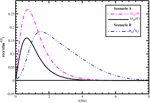
Figure 1: Wave functions. The pink dashed-dotted curve and the black solid curve represent the $\Delta\Delta$ components in the $d^{*}$ wave function in the framework of our chiral SU(3) constituent quark model with the single $\Delta\Delta$ (scenario A1) channel only and the coupled $\Delta\Delta+CC$ channel (scenario A2), respectively. The blue double-dotted-dashed curve shows the relative wave function of the ${}^{5}S_{2}$ component in $D_{12}$ with binding energy of $\epsilon=4.17~{}\rm{MeV}$.

In Fig. 1 and Table 1, one should notice that the $\Delta\Delta$ wave function in the coupled channel approximation is normalized to $0.31$. Clearly, we see that the wave function of $D_{12}$ is much more extended in radius in comparison with that of $\Delta\Delta$ does. This is reasonable, because the energy level of this state is fairly close to the $N\Delta$ threshold, the system is almost broken up, namely $N$ and $\Delta$ are ”almost free” and the separation between them becomes rather large. The smaller the binding energy is, the larger the size of the system would be. The root-mean-square radius of this component is $2.39~{}\rm{fm}$. This value is consistent with the prediction from Heisenberg uncertainty  Clement .

The charge distributions of the $d^{*}$ can be calculated by Eq. (17) in scenario A. The parameters $c_{m}$ and $b_{m}$ in Eq. (18) can be found in Refs. Dong ; Dong1 . The obtained charge distributions from $\Delta\Delta$ and $CC$ components are demonstrated in Fig. 2. The charge distribution of the single $\Delta\Delta$ model (scenario A1) is plotted in Fig. 2 by a pink dotted-dashed curve. The black solid and the red dashed curves denote the contributions from the $\Delta\Delta$ and $CC$ components (scenario A2), respectively, and the black dotted curve represents the total contribution by summing over former two curves. These curves tell us that the contribution from $CC$ component is larger than that from the $\Delta\Delta$ component, especially, in the larger momentum transfer region, the contribution is dominated by the $CC$ component. It implies that the quark contents in the $CC$ component tend to concentrate in a more compact region than that in the $\Delta\Delta$ component. This physics picture coincides with the radii of two components calculated in our previous paper Huang . Moreover, the curvature of the distribution curve of A1 is larger than that in the coupled channel case. It indicates that quarks here distribute in a larger region than that in the coupled channel case. The size information of $d^{*}$ can also be seen from the slope of the distribution curve at the origin, because such a slope is closely related to the radius of the system. The larger the slope at origin is, the larger the radius of the system would be. Comparing these slopes with the wave functions shown in Fig. 1, we find that the obtained slopes at the origin here coincide with the radii shown in Fig. 1. One sees that the radius resulted from the single channel wave function (A1) is larger than one from the two coupled-channel approximation (A2). Moreover, the radius contributed by the $CC$ component is smaller than the one from $\Delta\Delta$ component.

In order to see the size character of $d^{*}$ with a $D_{12}-\pi$ structure, the charge distribution of $d^{*}$ in the scenario B is calculated by Eq. (33). The obtained charge distribution curve, depicted by the blue double-dotted-dashed curve, is also drawn in Fig. 2 as well. It should be specially mentioned that in our numerical calculation, we do not solve the bound state problem for the $D_{12}\pi$ system, explicitly. However, since the requirement of the conservations of the total spin and parity, the relative motion between $D_{12}$ and $\pi$ must be at least a P-wave. Therefore, if we ignore the component with higher partial wave, which will be greatly suppressed, the true relative wave function would be a superposition of the P-wave wave functions with different size-parameters $\tilde{b}$. Thus, we calculate the charge distribution curves with a $\tilde{b}$ value from $0.6~{}fm$ to $6~{}fm$. The result shows that those curves almost overlap with each other, namely this curve is almost insensitive to the size-parameter $\tilde{b}$. This is because that the incoming photon is absorbed by the $D_{12}$ system, and the induced change of the relative momentum between the $D_{12}$ and $\pi$ is very small due to the factor of $m_{\pi}/\Big{(}M_{{}_{D_{12}}}+m_{\pi}\Big{)}\sim 6/100$. Comparing the curve of scenario B with others of scenario A, we see that the curves for the $D_{12}\pi$ scenario decrease and go to zero much faster than those for the scenario A. A much larger slope at the origin means that the radius of the $D_{12}\pi$ system is much larger in comparison with those in scenario A.

From our numerical calculation, we find that the ratios of the slopes of the curves at the origin in scenarios A1, A2, and B are

$$R=\Big{(}-\frac{\partial G_{E}^{A1}(Q^{2})}{\partial q^{2}}\Big{)}\Bigg{/}\Big{(}-\frac{\partial G_{E}^{A2}(Q^{2})}{\partial q^{2}}\Big{)}\Bigg{/}\Big{(}-\frac{\partial G_{E}^{B}(Q^{2})}{\partial q^{2}}\Big{)}\Bigg{/}\Bigg{|}_{Q^{2}=0}=2.30:1.45:6.86.$$ (35)

It should be mentioned that the contributions to $\frac{\partial G_{E}^{A1}(Q^{2})}{\partial q^{2}}$ from $\Delta\Delta$ and $CC$ components in the coupled channel approximation of Scenario A2 are 0.64 and 0.81, respectively. The above obtained ratios tell us that the slop of the charge distribution of the $d^{*}$ in scenario B at $Q^{2}=0$ is about 4.8 times larger than the one in Scenario A2, and the corresponding charge radius of scenario B is about 2.2 times larger than the one in scenario A2. This feature is compatable with that discussed in Ref. Gal1 . Finally, the very sharp charge distributions (or large charge radii) of $d^{*}(2380)$ in the scenario B is mainly dominated by the very broad wave function of the obtained $D_{12}$. Therefore, we conclude that the two scenarios, A2 and B for the $d^{*}(2380)$ give very different descriptions for its charge distribution and its charge radius.

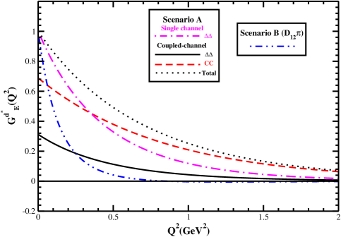
Figure 2: The obtained charge distributions of $d^{*}$. The solid(black), red(dashed), and black(dotted) curves stand for $\mid\Delta\Delta\chi_{\Delta}>$, $\mid cc\chi_{c}>$, and the $total$ contributions in the coupled channel approximation, respectively. The pink dotted-dashed curve represents the single channel case of scenario A. The blue double-dotted-dashed curves stand for the results of $D_{12}\pi$ scenario with $\epsilon\sim 4.17~{}\rm{MeV}$.

IV Summary

We have calculated the charge distribution of the $d^{*}$ in the two scenarios; one is a hexaquark dominant picture and another is a $D_{12}\pi$ resonant picture. In the first picture, we show the total charge distribution and both contributions from its $\Delta\Delta$ and $CC$ components. In order to make a comparison, the result of the single $\Delta\Delta$ channel is also shown. Comparing the predictions of the two scenarios, we see that the charge distribution from the $D_{12}\pi$ system is remarkably different from the scenario A2, and consequentially, the charge radius of the the scenario B is obviously larger than that of the scenario A2.

We now expect a series of experiments which may be able to test different interpretations of $d^{*}$ in future. Although the direct $ed^{*}$ scattering measurement may be hard to carry out, one may consider the $d^{*}$ form factors in the time-like region. For example, the production of the final $d^{*}\bar{d}^{*}$ pair in the $e^{+}e^{-}$ and $p\bar{p}$ annihilation processes. It is our hope that the future upgraded BEPC, Belle and Babar and experiment at $Panda$ with high luminosity may provide a test for different theoretical understandings.

- (1) M. Bashkanov et al., Phys. Rev. Lett. 102 052301 (2009).
- (2) P. Adlarson et al., Phys. Rev. Lett. 106, 242302 (2011); P. Adlarson et al., Phys. Lett. B 721, 229 (2013); P. Adlarson et al., Phys. Rev. Lett. 112, 202301 (2014).
- (3) A. Abashian, N. E. Booth, and K. W. Crowe, Phys. Rev. Lett. 5, 258 (1960); N. E. Booth, A. Abashian, and K. M. Crowe, Phys. Rev. Lett. 7, 35 (1961); F. Plouin et al., Nucl. Phys. A 302, 413 (1978), J. Banaigs et al., Nucl. Phys. B 105, 52 (1976).
- (4) M. Bashkanov, H. Clement, T. Skorodko, Eur. Phys. J. A51, 87 (2015).
- (5) COSY confirms existence of six-quark states, CERN COURIER, Vol. 54, No. 6, p6, July 23, 2014.
- (6) H. X. Chen, W. Chen, X. Liu and S. L. Zhu, Phys. Rept. 639, 1 (2016).
- (7) J. Dyson, Phys Rev. Lett. 13, 815 (1964).
- (8) A. W. Thomas, J. Phys. G 9, 1159 (1983).
- (9) M. Oka and K.Yazaki, Phys. Lett. B 90, 41 (1980).
- (10) T. Goldman et al., Phys. Rev. C 39, 1889 (1989).
- (11) X. Q. Yuan et al., Phys. Rev. C 60, 045203 (1999).
- (12) M. N. Platonova and V. I. Kukulin, Phys. Rev. C 87, 025202 (2013); Nucl. Phys. A 946, 117 (2016).
- (13) H. X. Huang et al. Phys. ReV. C 79, 024001 (2009); Phys. ReV. C 89, 034001 (2014).
- (14) A. Gal and H. Garcilazo, Phys Rev. Lett. 111, 172301 (2013); Nucl. Phys. A 928, 73 (2014); A. Gal, Acta Physica Polonica B 47, 471 (2016).
- (15) Fei Huang, Zongye Zhang, Pengnian Shen, and Wenling Wang, Chin. Phys. C39, 071001 (2015), Fei Huang, Pengnian Shen, Yubing Dong, and Zongye Zhang, Sci. China 59, 622002 (2016), and references therein.
- (16) Yubing Dong, Pengnian Shen, Fei Huang, and Zongye Zhang, Phys. Rev. C91, 064002 (2015).
- (17) Yubing Dong, Fei Huang, Pengnian Shen, and Zongye Zhang, Phys. Rev. C94, 014003 (2016).
- (18) Yubing Dong, Fei Huang, Pengnian Shen, and Zongye Zhang, ”Decay width of process in a chiral constituent quark model”, arXiv: 1702.03658v2 [nucl-th].
- (19) The WASA-at-COSY Collaboration, ”Isoscalar Single-Pion Production in the Region of Roper and Resonances” arXiv: 1702.07212V1 [nucl-ex].
- (20) M. Bashkanov, Stanley J. Brodsky, and H. Clement, Phys. Lett. B 727, 438 (2013).
- (21) H. Clement, ”On the History of Dibaryons and their Final Observation”, Progress in Particle and Nuclear Physics, 93, 195 (2017); arXiv:1610.0559v1 [Nucl-ex].
- (22) N. Barik, S. N. Jena, and D. P. Rath, Phys. Rev. D41, 1568 (1990).
- (23) S. R. Amendolia et al., Nucl. Phys. B277 (1986) 168.
- (24) A. Gal, ”The dibaryon resonance width and decay branching ratios”, arXiv:1612.05092, Phys. Lett. B, In Press.