On collisions times of ‘self-sorting’ interacting particles in one-dimension with random initial positions and velocities

Abstract

We investigate a one-dimensional system of $N$ particles, initially distributed with random positions and velocities, interacting through binary collisions. The collision rule is such that there is a time after which the $N$ particles do not interact and become sorted according to their velocities. When the collisions are elastic, we derive asymptotic distributions for the final collision time of a single particle and the final collision time of the system as the number of particles approaches infinity, under different assumptions for the initial distributions of the particles’ positions and velocities. For comparison, a numerical investigation is carried out to determine how a non-elastic collision rule, which conserves neither momentum nor energy, affects the median collision time of a particle and the median final collision time of the system.

1 Introduction

We consider a collection of $N$ ‘identical’ point-particles, with equal mass, moving on $\mathbb{R}$ and interacting through a linear binary collision rule given by

$$\begin{split}v_{i}^{\prime}&=(1-\epsilon)v_{j}\\ v_{j}^{\prime}&=(1-\epsilon)v_{i}.\\ \end{split}$$ (1)

Here $v_{i},v_{j}$ ($v_{i}^{\prime},v_{j}^{\prime}$) are the pre (post) collision velocities of particles $i$ and $j$ and the parameter $\epsilon<1$ controls conservation and dissipation of momentum and energy. Between collisions, particles undergo free flight. When $\epsilon=0$, a collision is elastic, preserving momentum and energy, and corresponds to an exchange of velocity between the two colliding particles. For $\epsilon\neq 0$, we refer to the collisions as non-elastic since Eq. (1) differs from the traditional construction of inelastic collisions which conserve momentum but not energy. In Section 1.2, we discuss the motivations for choosing Eq. (1) and its connection to standard inelastic collisions through a generalized linear collision framework. When $\epsilon<0$, collisions generate energy, and when $\epsilon\in(0,1)$ they dissipate energy. The case $\epsilon=1$ is degenerate, in the sense that particles stop their motion and remain ‘frozen’ together. For any $\epsilon<1$, as we show in Sections 1.1 and 1.2, each particle experiences a final collision, as eventually the velocities of all of the particles become sorted. In the above context, it is natural to ask (1) when a particle will experience its final collision, (2) when the final collision of the entire collection will occur, and (3) how these statistics depend on the initial position and velocity distributions, the number of particles in the system, and $\epsilon.$ The purpose of this article is to address these questions, analytically in the case of elastic collisions ($\epsilon=0$), and numerically for non-elastic collisions ($\epsilon\neq 0$).

The motivations for this work are twofold. First, in a recent article by Bardos et al [6], the long time limit of solutions to the Boltzmann equation over $\mathbb{R}^{d}$ was investigated. In the case of particles interacting through hard collisions, it was found that in unbounded domains, as opposed to bounded domains where the phenomenon is different, the dispersive effects of particle free flights were sufficient to quench the dissipative effects of collisions, thereby preventing the system from reaching a state of maximal entropy. Specifically, in terms of microscopic dynamics, one can envision a finite collection of particles in $\mathbb{R}^{d}$ with random initial positions and velocities. As time grows, the particles will likely spread out and interact with each other until a time when no more collisions occur. At this point, the system would be in a steady-state different from what might arise if the particles were kept confined to a bounded domain in $\mathbb{R}^{d}$. Therefore, from this view, understanding the final time of collision in the system is a natural question. Second, microscopic descriptions in terms of non-overlapping particles have proven to be central to the modeling of diffusion in single-file systems (see e.g. [13] and references therein), single-lane traffic flow [10], and self-organization in one-dimensional systems of self-propelled particles [9]. In this context, the system we study can be viewed as the microscopic equivalent of a one-dimensional gas of point particles, which interact through a generalized collision rule that is not necessarily subject to conservation of momentum or energy. A related example of dynamics on one-dimensional lattices includes the Stirring exclusion process [12].

Understanding the final collision time of a distinguished particle and the final collision time in a system of $N$ particles are questions about maximal order statistics for certain functions of the initial positions and velocities. Although we will assume the initial position and velocities of the particles are independent and identically distributed, when collisions are elastic, the collision times turn out to be an array of $\binom{N}{2}$ non-independent ‘exchangeable’ random variables without a finite mean. In this setting, we are able to analyze the collision times rigorously. When the collisions are non-elastic, however, an analytic approach is more difficult. As such, we use molecular dynamics simulations to assess the effects of non-elastic collisions on the collision times. In both non-elastic and elastic collisions, to avoid degeneracies, we will assume that the distributions of the initial positions and velocities are continuous random variables.

Informally, in the case of elastic collisions one set of our main results is that the final collision time of a distinguished particle, in the system of $N$ particles, depends on the moment properties of the position random variable (Theorems 1, 2, 3). That is, this final time scales with $N$ when the position r.v. has finite mean. It scales with $N^{1/\alpha}$ when the position r.v has the form of a symmetric stable law with parameter $0<\alpha<1$, and it scales with $N\log(N)$ when the position r.v. is a Cauchy distribution. In both of these cases, the limit distribution is a mixture of Fréchet distributions. Another set of our results concerns the final collision time $T^{(N)}$ for the whole system of $N$ particles. Here again, this time depends on how many moments the position r.v. possesses. In particular, when the latter has at least a $3/2$-moment, $T^{(N)}$ scales with $\binom{N}{2}$. When the position r.v. has the form of a stable symmetric law with parameter $0<\alpha<1$, $T^{(N)}$ scales with $N^{2/\alpha}$, and when the position r.v. is a Cauchy distribution, $T^{(N)}$ scales with $N^{2}\log N$. In each of these cases, the limit is of Fréchet type (Theorems 4, 5, 6). However, we also show that when the position r.v. has a first moment, the sequence of final collision times for $N\geq 2$ is tight in the scale $\binom{N}{2}$ (Proposition 2). Moreover, some numerical simulations are provided which indicate that the result of Theorem 4 should extend to the case when the position r.v. has a mean without further restrictions.

For non-elastic collisions, we present numerical results in the case where the initial positions are standard normal distributions. Numerical simulations indicate that, unlike elastic collisions, the final collision time of a distinguished particle does not scale with $N$, and the final collision time of the system does not scale with $N^{2}$. Instead, both times require an exponential correction depending on $N\epsilon$ ad the initial distribution of velocities. An ansatz is discussed which offers a limited explanation to the observed changes.

An outcome of this work is the formulation of a ‘sorting model’ through which the collision times under elastic interactions can be conveniently analyzed. In this elastic interaction framework, the $\binom{N}{2}$ collision times are understood through methods for exchangeable arrays. Various types of these arrays have been considered in [7, 5, 11, 14]. From the perspective of colliding particles, this work is related to a different collection of processes, where the initial positions are nonrandom, but the particles interact randomly, which was considered in [1, 2, 3, 4].

The rest of this article is organized as follows. We now state precisely, in the next subsection, the setting and the main quantities of interest, recast the space-time dynamics of the $N$ particles in terms of a ‘sorting process’, and formulate the questions studied with respect to elastic collisions. In subsection 1.2, we prove the existence of a final collision time under non-elastic collisions ($\epsilon\neq 0$). In Section 2, we state the main theorems for elastic collisions. In Section 3, we discuss numerical results for non-elastic collisions. Finally, the proofs of theorem 1, 2, 4, and 5 are given in Section 4. As the proofs of theorems 3 and 6 are similar in structure to those of theorems 2 and 5, we have elected to include them in an appendix.

1.1 Elastic collisions on the line as a sorting process

Consider $N$ point particles with equal mass and initial positions $\{X_{i}\}_{i=1}^{N}$, which are assumed to be independent, identically distributed random variables with density $f_{x}$. The initial velocities of the particles are denoted by $\{V_{i}\}_{i=1}^{N}$ and are also assumed to be independent, identically distributed random variables with continuous, bounded density $f_{v}$. In particular, almost surely, no two particles have the same position or velocity. Between collisions, particles undergo free flight.

We start by proving that all collisions occur within a finite time $T^{(N)}$, as long as $N$ remains finite. Since an elastic collision corresponds to an exchange of velocities between the colliding particles, switching particle labels during collisions turns each labelled trajectory into a straight line. This point of view gives a simple way of calculating all the collision times, past and present, in terms of the initial data only. Indeed, let $\ell_{i}(t)=X_{i}+tV_{i}$ denote the labelled trajectory of the $i$th particle, and $\tau_{i,j}$ denote the time of intercept of the paths $\ell_{i}(\cdot)$ and $\ell_{j}(\cdot)$ of particles $i$ and $j$. Then,

$$\tau_{i,j}=\frac{X_{j}-X_{i}}{V_{i}-V_{j}}$$

and the set of all the line intersection times, $\{\tau_{i,j}:1\leq i\neq j\leq N\}$ is in one-to-one correspondence with the set of all collision times of the particles undergoing elastic collisions if we consider both positive and negative times. We remark, since the distributions of the initial positions and velocity are continuous, these times are distinct almost surely. Also, although these intersection times are not independent random variables, for example $\tau_{1,2}$ and $\tau_{1,3}$ both depend on $(X_{1},V_{1})$, they are ‘exchangeable’ in the sense that if $\pi$ is a permutation of $\{1,\ldots,N\}$, then $\{\tau_{i,j}:1\leq i\neq j\leq N\}\mathop{=}\limits^{d}\{\tau_{\pi(i),\pi(j)}:1\leq i\neq j\leq N\}$. The intersection times, $\tau_{i,j}$, are examples of ratio distributions. One can construct an integral representation of the distribution of such a ratio, although evaluating the integral in closed form is often difficult. However, for example, if $\{X_{i}\}_{i=1}^{N}$ and $\{V_{i}\}_{i=1}^{N}$ are all iid $N(\mu,\sigma)$, then any $\tau_{i,j}$ follows a Cauchy distribution.

As the collection of collision times consists of $\binom{N}{2}$ terms, after the final (random) time $T{\color[rgb]{0,0,0}\definecolor[named]{pgfstrokecolor}{rgb}{0,0,0}\pgfsys@color@gray@stroke{0}\pgfsys@color@gray@fill{0}^{(N)}}:=\max_{i\neq j}\tau_{i,j}$, there will be no more collisions between particles. After this time, the labels of the lines have been sorted according to their velocities: in a vertical cross-section of the space time diagram, they are, from top to bottom, in order from the largest to the smallest initial velocities. Similarly, after time $T^{(N)}$, all particles are arranged on the one-dimensional line in order of increasing speed, moving only by free flight since no further collisions can occur.

Let $t_{i}^{(N)}$ be the last time the $i$th particle interacts with any other particle. Since the initial positions and velocities are independent and identically distributed, the random variables $\{t_{i}^{(N)}:1\leq i\leq N\}$ are exchangeable, although not independent. On the other hand, let $r_{i}^{(N)}:=\max_{j:j\neq i}\tau_{i,j}$ denote the last time another line intersects $\ell_{i}(\cdot)$. Then, as the last collision time of a particle must be the last intersection time of a line, we have $\{t_{i}^{(N)}:1\leq i\leq N\}\mathop{=}\limits^{d}\{r_{i}^{(N)}:1\leq i\leq N\}$. Moreover, as the initial positions and velocities are independent, $r^{(N)}_{i}$ equals any one of the $\{t_{i}^{(N)}:1\leq i\leq N\}$ with equal probability. In particular,

$$P(r_{i}^{(N)}\leq x)=N^{-1}\sum_{j=1}^{N}P(t_{j}^{(N)}\leq x)=P(t_{i}^{(N)}\leq x),$$

and so $t_{i}^{(N)}$ and $r_{i}^{(N)}$ have the same distribution. Also,

$$T^{(N)}=\max_{1\leq i\leq N}r_{i}^{(N)}=\max_{1\leq i\leq N}t_{i}^{(N)}.$$

Although not discussed here, we remark that it is also natural to consider, as an alternative, the minimum of the collision times. Given the symmetric distribution of $\tau_{i,j}$ it follows that

$$\min_{1\leq i<j\leq N}\tau_{i,j}\mathop{=}\limits^{d}-T^{(N)}.$$

1.2 Non-elastic collisions

Consider the more general, linear inelastic collision rule

$$\begin{split}v_{i}^{\prime}&=(1-\epsilon)v_{j}{\color[rgb]{0,0,0}\definecolor[named]{pgfstrokecolor}{rgb}{0,0,0}\pgfsys@color@gray@stroke{0}\pgfsys@color@gray@fill{0}+\beta v_{i},}\\ v_{j}^{\prime}&=(1-\epsilon)v_{i}{\color[rgb]{0,0,0}\definecolor[named]{pgfstrokecolor}{rgb}{0,0,0}\pgfsys@color@gray@stroke{0}\pgfsys@color@gray@fill{0}+\beta v_{j}}.\end{split}$$ (2)

Recall that $v_{i},v_{j}$ ($v_{i}^{\prime},v_{j}^{\prime}$) are the pre (post) collision velocities of particles $i$ and $j$. The parameters ${\color[rgb]{0,0,0}\definecolor[named]{pgfstrokecolor}{rgb}{0,0,0}\pgfsys@color@gray@stroke{0}\pgfsys@color@gray@fill{0}\beta\geq\ }0$ and $\epsilon<1$ control conservation and dissipation of momentum and energy. In the case $\beta=\epsilon\neq 0$, Eq. (2) corresponds to inelastic collisions with coefficient of restitution $C_{R}=1-2\epsilon$, which conserve momentum but not energy. In what follows we choose $\beta=0$ to reduce the computational cost of the simulations, thereby making the large numerical study from Sec. 3 possible. The simplicity of the collision rule obtained when $\beta=0$ allows for some analytic investigation as well. Moreover, since reversing the direction of time when a collision occurs amounts to changing $\epsilon$ into $1-\frac{1}{1-\epsilon}\simeq-\epsilon$ at leading order when $\epsilon$ is small, the distributions of collision times are, for small values of $\epsilon$, expected to be nearly symmetric under the transformation $\cal T$ sending $t\to-t$ and $\epsilon\to-\epsilon$. This is confirmed by the simulations of Fig. 1, which interestingly indicate that the symmetry under $\cal T$ is qualitatively observed, even for values of $\epsilon$ equal to 0.1. We also note that, the transformation $\cal T$ can be used to understand properties of the minimum order statistics of the collision times through study of $t_{i}^{(N)}$ and $T^{(N)}$. As already mentioned, the pairwise collision times display a system size dependency which is not present for elastic collisions. Together with the broken symmetry, this effect can be viewed as resulting from the cooling (heating) of the system in the case of energy dissipating (generating) collisions: a greater number of particles results in more collisions, which is compounded into increased cooling (or heating).

Figure 1: Histograms of collision times $\tau_{i,j}$ for positive (left) and negative (right) values of $\epsilon$ in the non-elastic collision rule (1) with $\beta=0$. The initial positions and velocities are sampled from a standard normal distribution. For comparison, the densities of collision times for elastic collisions are shown in dashed red. In this case, the elastic collision times follow a Cauchy distribution.

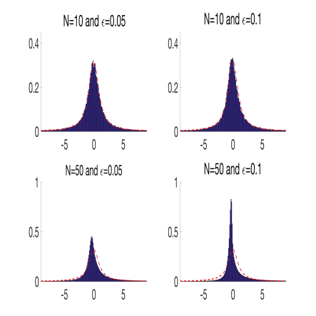
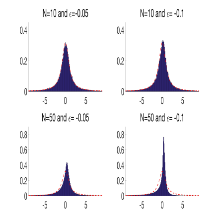
For elastic collisions, the one-to-one correspondence of path intersection times and collision times made the argument for the existence of a final collision time straightforward. For non-elastic collisions, the existence of a final collision time is less obvious. Nonetheless, the proposition below indicates there is almost surely a final collision time for a system of particles interacting with the collision rule from Eq. (1) when $\epsilon<1$.

Proposition 1.

Suppose $N$ point particles with equal mass have initial positions $\{X_{i}\}_{i=1}^{N}$ and velocities $\{V_{i}\}_{i=1}^{N}$ that are continuous random variables, so that $X_{i}\neq X_{j}$, $V_{i}\neq V_{j}$ for $i\neq j$ a.s. If the particles interact through the collision rule given in Eq. (1) with $\epsilon\neq 0,\ \epsilon<1$, there is a final collision time almost surely.

Proof .

Suppose at the time of a collision, in addition to the change in velocity, the labels of particles are also switched. Unlike the case of elastic collisions, the path of a particle in space-time is not a straight line. Instead, individual particles follow piecewise linear trajectories where the slope of each segment changes by a factor of $1-\epsilon$ after each intersection with another path. Again, let $\ell_{i}(t)$ denote the position of the $i$th particle and $\tau_{i,\star_{1}}<\tau_{i,\star_{2}}<\dots$ denote the times when the path of particle $i$ intercepts the path of another particle. Then

$$\ell_{i}(t)=\begin{cases}X_{i}+tV_{i}&0<t\leq\tau_{i,\star_{1}}\\ (X_{i}+\tau_{i,\star_{1}}V_{1})+(t-\tau_{i,\star_{1}})(1-\epsilon)V_{i}&\tau_{i,\star_{1}}<t\leq\tau_{i,\star_{2}}\\ \vdots\end{cases}$$

As was the case for elastic collisions, the collection of intersection times of the trajectories of particles (now piecewise linear) is in one-to-one correspondence with the collection of collision times. Therefore, for a system to have infinitely many collision times, there must be two paths which intersect infinitely many times. Since the initial velocities are continuous random variables, it follows that for all $1\leq i<j\leq N$ and $k,m\in\{0,1,2,\dots\}$, $(1-\epsilon)^{k}V_{i}\neq(1-\epsilon)^{m}V_{j}$ almost surely which ensures that any two paths which intersect do so by crossing one another a.s.

We now assume the paths $\ell_{1}$ and $\ell_{2}$ intersect infinitely often and derive a contradiction. Since the paths cross, we may choose two successive intersection times, $s_{1}^{(2)}<s_{2}^{(2)}$, such that $\ell_{1}(t)>\ell_{2}(t)$ for $t\in(s_{1}^{(2)},s_{2}^{(2)})=\mathbb{S}^{(2)}.$ It may be the case that a third path also intersects $\ell_{1}$ and $\ell_{2}$ at time $s_{1}^{(2)}$ or $s_{2}^{(2)}$. However, we may relabel the paths so that a ternary intersection does not alter the velocities of paths $\ell_{1}$ and $\ell_{2}$ on the open interval $\mathbb{S}^{(2)}.$

For example, suppose $\ell_{3}$ also intersects with $\ell_{1}$ and $\ell_{2}$ at $s_{1}^{(2)}$ or $s_{2}^{(2)}$. There are two possibilities. Firstly, $\ell_{3}$ does not intersect $\ell_{1}$ or $\ell_{2}$ on the interval $(s_{1}^{(2)},s_{2}^{(2)}).$ Thus, $\ell_{3}$ will not alter the velocities of $\ell_{1},\ell_{2}$ on this interval and so will not influence the time, $s_{2}^{(2)}$, when $\ell_{1}$ and $\ell_{2}$ intersect again.

Secondly, $\ell_{3}$ could intersect either $\ell_{1}$ or $\ell_{2}$ at a second time $s\in(s_{1}^{(2)},s_{2}^{(2)}).$ For instance, suppose $\ell_{3}$ intersects with $\ell_{1}$ at times $s$ and $s_{2}^{(2)}$, and that $\ell_{3}$ does not intersect $\ell_{2}$ on the interval $(s,s_{2}^{(2)}).$ We can then relabel the paths and times so that, $\ell_{1}$ and $\ell_{2}$ (formerly $\ell_{1}$ and $\ell_{3}$), intersect at successive times $s_{1}^{(2)}$ and $s_{2}^{(2)}$ (formerly $s$ and $s_{2}^{(2)}$). Then on the interval $(s_{1}^{(2)},s_{2}^{(2)})$, the path $\ell_{3}$ (formerly $\ell_{2}$) intersects with neither $\ell_{1}$ nor $\ell_{3}$. Other possibilities are handled similarly. As a result of this choice, on the closed interval $\overline{\mathbb{S}^{(2)}}$, any path which crosses both $\ell_{1}$ and $\ell_{2}$ does so an equal number of times.

Let us return to case where $\ell_{1}$ and $\ell_{2}$ intersect at successive times $s_{2}^{(1)}$ and $s_{2}^{(2)}$ and $\ell_{1}(t)>\ell_{2}(t)$ for $t\in\mathbb{S}^{(2)}$. Furthermore, assume these paths are chosen so that there is no other path which intersects both $\ell_{1}$ or $\ell_{2}$ at $s_{1}^{(2)}$ or $s_{2}^{(2)}$ and either $\ell_{1}$ or $\ell_{2}$ at another time in the interval $\mathbb{S}^{(2)}.$ Let

$$u_{i}^{+}=\lim_{h\to 0^{+}}\frac{\ell_{i}(s_{1}^{(2)}+h)-\ell_{i}(s_{1}^{(2)})}{h},\hskip 5.69054pti=1,2\\$$

be the velocities of particles $1$ and $2$ immediately after their collision at $s_{1}^{(2)}.$ Let

$$U_{i}^{-}=\lim_{h\to 0^{-}}\frac{\ell_{i}(s_{2}^{(2)}+h)-\ell_{i}(s_{2}^{(2)})}{h},\hskip 5.69054pti=1,2\\$$

be the velocities of particles $1$ and $2$ immediately before their collision at $s_{2}^{(2)}.$ Since $\ell_{1}(t)>\ell_{2}(t)$ for $t\in\mathbb{S}^{(2)}$ and the paths cross a.s., it follows that

$$u_{1}^{+}>u_{2}^{+}\hskip 5.69054pt\text{ and }\hskip 5.69054ptU_{1}^{-}<U_{2}^{-}\hskip 5.69054pt\text{ a.s}.$$ (3)

We note that the velocities of both paths $1$ and $2$ must be of the same sign since $U_{i}^{-}$ is related to $u_{i}^{+}$ by the equation $U_{i}^{-}=(1-\epsilon)^{k_{i}}u_{i}^{+}$ where $(1-\epsilon)^{k_{1}}>0$ and $k_{i}$ is the number of additional path intersections of $i$ during $\mathbb{S}^{(2)}$.

Consider the path intersections involving $\ell_{1}$ on the interval $\mathbb{S}^{(2)}$ (Fig. 2). There are two possibilities. (1) A path, (shown as a dotted, red line in Fig. 2), crosses both $\ell_{1}$ and $\ell_{2}$ (the dashed, blue lines in Fig. 2) $k$ times, and alters the velocities of both particles by a multiplicative factor of $(1-\epsilon)^{k}.$ Alternatively, (2) a path may only intersect $\ell_{1}$ leaving the velocity of particle 2 unchanged (the solid black line in Fig. 2).

Figure 2: Paths $\ell_{1}$ and $\ell_{2}$ are shown as dashed, blue lines. The dotted red line serves as an example of a path which intersects both $\ell_{1}$ and $\ell_{2}$. A path which intersects $\ell_{1}$ twice without hitting $\ell_{k}$ (shown as a solid black line) implies the existence of another ‘nested’ path, $\ell_{k+1}$, also crossing $\ell_{1}$ twice but between the times, $s_{1}^{(k)}<s_{2}^{(k)}$, when $\ell_{k}$ hits $\ell_{1}$.

If only $k_{1}$ intersections of the first type occur, then

$$U_{1}^{-}=u_{1}^{+}(1-\epsilon)^{k_{1}}>u_{2}^{+}(1-\epsilon)^{k_{1}}=U_{2}^{-}$$

which contradicts the assumption that $U_{1}^{-}<U_{2}^{-}.$ Indeed, $\ell_{1}$ and $\ell_{2}$ must experience a different number of intersections, $k_{1}$ and $k_{2}$ respectively, so that

$$U_{1}^{-}=(1-\epsilon)^{k_{1}}u_{1}^{+}<(1-\epsilon)^{k_{2}}u_{2}^{+}=U_{2}^{-}.$$

The details of the ordering of $k_{1}$ and $k_{2}$ depend on both the sign of $u_{1}^{+},u_{2}^{+}$ and on the sign of $\epsilon.$ However, we may assume without loss of generality that $k_{1}>k_{2}\geq 0.$

Thus, there must be a path which intersects $\ell_{1}$ at least twice without intersecting $\ell_{2}$. Call it $\ell_{3}$. Again, we may choose successive intersection times, $s_{1}^{(3)}<s_{2}^{(3)}$ in $\mathbb{S}^{(2)},$ such that $\ell_{1}(t)>\ell_{3}(t)$ and repeat the preceding argument (Fig. 2).

As such, the existence of a $k$th path with successive intersections of $\ell_{1}$ at times $s_{1}^{(k)}<s_{2}^{(k)}$ then implies the existence of a $(k+1)$th path which has successive intersections with $\ell_{1}$ on a subinterval $\mathbb{S}^{(k+1)}=(s_{1}^{(k+1)},s_{2}^{(k+1)})\subset(s_{1}^{(k)},s_{2}^{(k)})=\mathbb{S}^{(k)}$. By construction, $\ell_{2},\dots,\ell_{k}$ cannot collide with $\ell_{1}$ on $\mathbb{S}^{(k+1)}$. Through induction we reach a contradiction as this requires an $(N+1)$th path in a system with only $N$ paths.

∎

Like in the system with elastic collisions discussed above, collisions stop once particles become sorted in order of increasing velocity. However, the distribution of velocities of the particles is no longer independent of collisions, but instead depends on the number of collisions that each particle experiences.

2 Results for Elastic Collisions

2.1 Final Collision Time for a Single Particle

The first theorem concerns the setting where $E|X_{1}|<\infty$. In this case, the initial position of the center of mass of the system of particles converges to a constant value a.s. as $N$ tends towards infinity.

Theorem 1.

Let $t_{i}^{(N)}=\max_{i\neq j}\tau_{i,j}$ be the final path intersection time for a single particle in a system of $N$ particles with iid initial position $\{X_{i}\}_{i=1}^{N}$ with density $f_{x}$ and iid initial velocities $\{V_{i}\}{\color[rgb]{0,0,0}\definecolor[named]{pgfstrokecolor}{rgb}{0,0,0}\pgfsys@color@gray@stroke{0}\pgfsys@color@gray@fill{0}_{i=1}^{N}}$ with density $f_{v}$. Suppose $E|X_{1}|<\infty$ and that $f_{v}$ is continuous and bounded. Then, for $\mu>0$,

$$\lim_{N\to\infty}P\bigg{(}\frac{t_{i}^{(N)}}{N}<\mu\bigg{)}=\int_{\mathbb{R}^{2}}f_{x}(X)f_{v}(V)e^{-\frac{C(X,V)}{\mu}}dXdV$$

where

$$C(X,V)=f_{v}(V)\int_{\mathbb{R}}|X-y|f_{x}(y)dy.$$

In other words, the period of time during which each point particle undergoes elastic collisions scales linearly with the size $N$ of the system, as long as the position of the center of mass of the system remains finite. For example, if the positions and velocities are iid $U[-1/2,1/2]$, then

$$\lim_{N\to\infty}P\bigg{(}\frac{t_{i}^{(N)}}{N}<\mu\bigg{)}=\begin{cases}e^{-\frac{1}{4\mu}}\int_{-1/2}^{1/2}e^{-x^{2}/\mu}dx&\mu>0\\ 0&\mu\leq 0.\end{cases}$$

Theorems 2 and 3 consider when $X_{1}$ does not have mean, or, when the initial position of the center of mass of the system of particles does not converge a.s. as $N$ tends towards infinity. In this case, we require different rescalings of $t_{i}^{(N)}$ depending on the behavior of the tail of the distribution of $X_{1}.$

Theorem 2.

Let $t_{i}^{(N)}$ and $f_{v}$ be as in Thm. 1. Suppose $\{X_{i}\}_{i=1}^{N}$ are iid with density $f_{x}(X)=\frac{C_{\alpha}}{1+|x|^{1+\alpha}}$ for some $\alpha\in(0,1)$. Then, for $\mu>0,$

$$\lim_{N\to\infty}P\bigg{(}\frac{t_{i}^{(N)}}{N^{1/\alpha}}<\mu\bigg{)}=\int_{\mathbb{R}}f_{v}(V)\exp\bigg{(}-\frac{C(V)}{\mu^{\alpha}}\bigg{)}dV$$

where

$$C(V)=\frac{C_{\alpha}}{\alpha}\int_{\mathbb{R}}f_{v}(V+w)\frac{1}{|w|^{\alpha}}dw.$$

Theorem 3.

Let $t_{i}^{(N)}$ and $f_{v}$ be as in Thm. 1. Suppose $\{X_{i}\}_{i=1}^{N}$ are iid Cauchy random variables. Then, for $\mu>0,$

$$\lim_{N\to\infty}P\bigg{(}\frac{t_{i}^{(N)}}{N\log N}\leq\mu\bigg{)}=\int_{\mathbb{R}}f_{v}(V)\exp\bigg{(}-\frac{2f_{v}(V)}{\pi\mu}\bigg{)}dV.$$

We remark, in passing, that in the event $f_{x}(z)$ has different scalings as $z\to\pm\infty$, one can still construct asymptotic distributions of $t_{i}^{(N)}$. The more slowly decaying tail will dominate the asymptotic behavior and the distribution will look similar to the result from Thm. 2 or Thm. 3 depending on the details of $f_{x}.$ The proofs of the above theorems are provided in Section 4.1.

2.2 Final Collision Time of the System

We now turn to the scaling properties of $T^{(N)}$. Again, the first theorem presented concerns the situation when $X_{1}$ has a finite mean. We will in fact require that the position distribution has at least a $3/2$-moment for technical reasons; details of this proof are discussed in Sec. 4.2.

Theorem 4.

Let $T^{(N)}=\max\limits_{1\leq i<j\leq N}\tau_{i,j}$ be the final collision time of a collection of $N$ particles. Suppose $E|X_{1}|^{3/2}<\infty$ and that $f_{v}$ is continuous and bounded. Then, for $t>0$,

$${\color[rgb]{0,0,0}\definecolor[named]{pgfstrokecolor}{rgb}{0,0,0}\pgfsys@color@gray@stroke{0}\pgfsys@color@gray@fill{0}\lim_{N\to\infty}}P\bigg{(}\frac{T^{(N)}}{\binom{N}{2}}\leq t\bigg{)}{\color[rgb]{0,0,0}\definecolor[named]{pgfstrokecolor}{rgb}{0,0,0}\pgfsys@color@gray@stroke{0}\pgfsys@color@gray@fill{0}=\ }e^{-C/t},$$

where

$$C=\int_{\mathbb{R}^{2}}|x-y|\,f_{x}(x)\,f_{x}(y)\,dx\,dy\cdot\int_{\mathbb{R}}f_{v}^{2}(v)\,dv.$$

This indicates that the final collision time of the system scales like the total number of particle pairs. The numerical simulation of Figure 3 illustrates the convergence of the cumulative distribution of $T^{(N)}/\binom{N}{2}$ towards its asymptotic value on the interval $t\in(0,5)$ when both $\{X_{i}\}_{i=1}^{N}$ and $\{V_{i}\}_{i=1}^{N}$ are iid $N(0,1)$. The Silverman-Brown limit law used in the proof shown in Section 4.2 indicates that the rate of convergence is $O(N^{-1})$, which is consistent with the numerical results. In order to numerically observe this rate of convergence, a total of $N^{4}$ trials had to be conducted to reconstruct the cumulative distribution of $T^{(N)}$.

Figure 3: The maximum difference between the empirical cumulative distribution function and theoretical asymptotic cumulative distribution function of $T^{(N)}/\binom{N}{2}$ over all values $t$ in the interval $(0,5)$ when both $\{X_{i}\}_{i=1}^{N}$ and $\{V_{i}\}_{i=1}^{N}$ are iid $N(0,1)$ with system sizes, $N$, between 5 and 100. For reference, the dashed line has slope negative one.

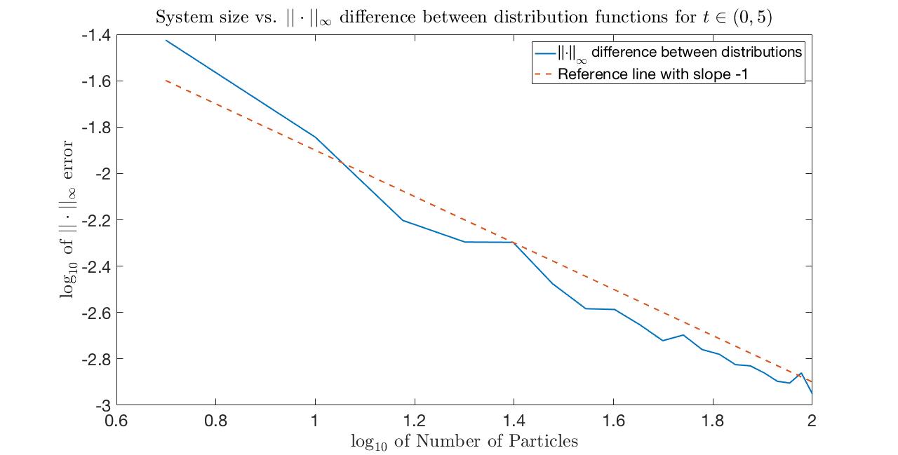
Two points are worth noting regarding the proof of Thm. 4. First, since both $\{X_{i}\}_{i=1}^{N}$ and $\{V_{i}\}_{i=1}^{N}$ are identically distributed, the intersection times $\tau_{i,j}$ are also identically distributed. However, they are not independent. Nonetheless, if one assumes they are independent, then through the usual construction of the maximal order statistics of i.i.d. random variables, one recovers the same distribution as in Thm. 4 as $N\to\infty.$ Second, although the proof of the theorem requires that $E|X_{1}|^{3/2}<\infty$ for technical reasons, it is natural to wonder if $T^{(N)}/\binom{N}{2}$ is still converging weakly to some random variable if the requirements of the moment of $X_{1}$ are lessened.

Proposition 2.

Suppose $E|X_{1}|<\infty$ and $f_{v}$ is continuous and bounded, then the sequence of random variables $\{T^{(N)}/\binom{N}{2}\}_{N=2}^{\infty}$ is tight.

A proof of this proposition is given in Sec. 4.2. Since the sequence, $\{T^{(N)}/\binom{N}{2}\}_{N=2}^{\infty}$ is tight, there is a random variable $T$ and subsequence $N_{j}$ such that

$$\frac{T^{(N_{j})}}{\binom{N_{j}}{2}}\Rightarrow T.$$

In the case of Thm. 4, the asymptotic distribution of $T^{(N)}/\binom{N}{2}$ is known. However, the tightness of the sequence $\{T^{(N)}/\binom{N}{2}\}$ requires only that $E|X_{1}|<\infty$, a condition which also guarantees the constant $C$ of Thm. 4 is well-defined.

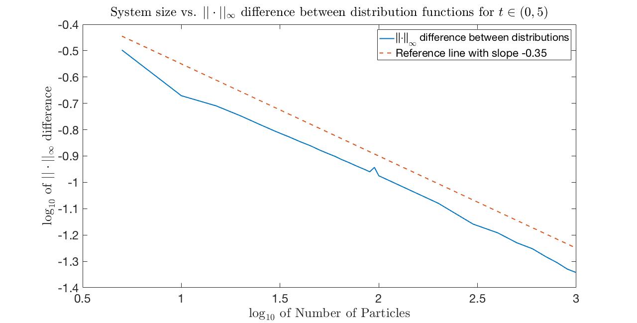
It is natural to ask whether the limiting distribution given in Thm. 4 still holds if the requirement that $E|X_{1}|^{3/2}{\color[rgb]{0,0,0}\definecolor[named]{pgfstrokecolor}{rgb}{0,0,0}\pgfsys@color@gray@stroke{0}\pgfsys@color@gray@fill{0}<\infty}$ is removed. Even though we do not provide a definite answer to this question, the following example gives some insight. We simulated systems of increasing size $N$, with random initial positions $\{X_{i}\}_{i=1}^{N}$ generated, via inverse sampling, from the density

$$f_{x}(x)=\frac{9\cos(\pi/18)}{8\pi(1+|x|^{9/4})},$$ (4)

for which $E|X_{1}|<\infty$ but $E|X_{1}|^{\alpha}$ is infinite for $\alpha\geq 5/4$. Random initial velocities were sampled from a $N(0,1)$ distribution. Figure 4 shows a comparison between the empirical and theoretical cumulative distribution functions, similar to the example of Fig. 3, but for a larger range of values of $N$. The distribution of $T^{(N)}/\binom{N}{2}$ appears to be converging to the same theoretical limit as Thm. 4, but at a much slower rate, of order $O(N^{-0.35})$. This suggests that an argument for the convergence of $T^{(N)}$ to the same limiting distribution may exist for this example. However, we show in the appendix that the method of proof we use cannot apply in this case.

Figure 4: The maximum difference between the empirical cumulative distribution function and theoretical asymptotic cumulative distribution function of $T^{(N)}/\binom{N}{2}$ in the infinity norm over the interval $\mu\in(0,5)$. Here, $\{X_{i}\}_{i=1}$ are iid with density given in Eq. (4), $\{V_{i}\}_{i=1}^{N}$ are iid $N(0,1)$, and the size of the system, $N$, ranges between 5 and 1000. For reference, the dashed line has slope of -0.35. For $N$ between 5 and 100, $N^{4}$ trials were conducted. Over that interval the observed convergence rate was $N^{-0.35}$. As such, only $N^{2}$ trials were conducted for systems sizes between 100 and 1000.

We now discuss asymptotic distributions for $T^{(N)}$ when the initial position r.v. does not have a first moment. Similar to Theorems 2 and 3 an alternate scaling is required.

Theorem 5.

Let $T^{(N)}$ be the final collision time of a collection of $N$ particles. Suppose the initial positions are iid with density $\displaystyle f_{x}(x)=\frac{C_{\alpha}}{1+{\color[rgb]{0,0,0}\definecolor[named]{pgfstrokecolor}{rgb}{0,0,0}\pgfsys@color@gray@stroke{0}\pgfsys@color@gray@fill{0}|x|}^{1+\alpha}}$ for $\alpha\in(0,1)$ and that $f_{v}$ is continuous and bounded. Then for $t>0$,

$${\color[rgb]{0,0,0}\definecolor[named]{pgfstrokecolor}{rgb}{0,0,0}\pgfsys@color@gray@stroke{0}\pgfsys@color@gray@fill{0}\lim_{N\to\infty}}P\bigg{(}\frac{T^{(N)}}{N^{2/\alpha}}\leq t\bigg{)}{\color[rgb]{0,0,0}\definecolor[named]{pgfstrokecolor}{rgb}{0,0,0}\pgfsys@color@gray@stroke{0}\pgfsys@color@gray@fill{0}=\ }e^{-C/t^{\alpha}}$$

where

$$C=\frac{C_{\alpha}}{2\alpha}\int_{\mathbb{R}^{2}}f_{v}(V)\frac{f_{v}(V+w)}{|w|^{\alpha}}dw\,dV.$$

Theorem 6.

Let $T^{(N)}$ be the final collision time of a collection of $N$ particles. Suppose the initial positions are iid Cauchy and that $f_{v}$ is continuous and bounded. Then for $t>0$,

$${\color[rgb]{0,0,0}\definecolor[named]{pgfstrokecolor}{rgb}{0,0,0}\pgfsys@color@gray@stroke{0}\pgfsys@color@gray@fill{0}\lim_{N\to\infty}}P\bigg{(}\frac{T^{(N)}}{N^{2}\log N}\leq t\bigg{)}{\color[rgb]{0,0,0}\definecolor[named]{pgfstrokecolor}{rgb}{0,0,0}\pgfsys@color@gray@stroke{0}\pgfsys@color@gray@fill{0}=\ }e^{-C/t}$$

where

$$C=\frac{{\color[rgb]{0,0,0}\definecolor[named]{pgfstrokecolor}{rgb}{0,0,0}\pgfsys@color@gray@stroke{0}\pgfsys@color@gray@fill{0}2}}{\pi}\int_{\mathbb{R}}f_{v}^{2}(V)dV.$$

Like Theorem 4, the limiting distributions in Theorems 5 and 6 are of Fréchet type. Additionally, as was the case for Theorem 4, one recovers the same asymptotic distribution if the pairwise collision times are assumed to be independent. The proofs of these theorems follow from the same asymptotic arguments employed in the proofs of Theorems 2 and 3 which are discussed in detail in Section 4.1 and in the Appendix.

In summary, the asymptotic properties of $T^{(N)}$ depend on the moment properties of the initial position r.v. In the simple case where the initial velocity r.v. has a continuous density and the initial position r.v. has a density of the form $f_{x}(x)=\frac{C_{\alpha}}{1+|x|^{1+\alpha}}$, we have the following results: for $\alpha\in(0,1)$, Theorem 5 holds and $T^{(N)}$ scales like $N^{2/\alpha}$; for $\alpha=1$, Theorem 6 holds and $T^{(N)}$ scales like $N^{2}\log N$; and for $\alpha>3/2$ Theorem 4 holds and $T^{(N)}$ scales like $N^{2}$. As mentioned earlier, the case for $\alpha\in(1,3/2]$ is open, but the numerical study of Fig. 4 suggests the result of Theorem 4 still holds and $T^{(N)}$ scales like $N^{2}$.

3 Results for Non-elastic Collisions

The presence of non-elastic collisions ($\epsilon\neq 0$) significantly affects the asymptotic behavior of the system. First, due in part to the heating/cooling effects observed in Sec. 1.2, the asymptotic properties of $t_{i}^{(N)}$ and $T^{(N)}$ are modified. Importantly, the initial velocity distribution plays a role, which was not the case for elastic collisions, whose asymptotic behavior was solely determined by the distribution of initial positions. Second, the analytic framework we used to determine the correct asymptotic behavior of $t_{i}^{(N)}$ and $T^{(N)}$ is no longer viable. As a consequence, we do not have the means to rigorously derive the asymptotic distributions of these quantities at this time. Instead, we describe how their medians scale through a numerical study using molecular dynamics (MD) simulations.

Since under elastic collisions, neither the limiting distribution of $t_{i}^{(N)}/N$ nor that of $T^{(N)}/N^{2}$ has a mean, we assume this is also the case under non-elastic collisions. We thus investigate how the medians of $t_{i}^{(N)}$ and $T^{(N)}$ scale for large $N$. We restrict our focus to $N(0,1)$ initial position distributions, and study separate cases when the initial velocities are iid $N(0,1)$, $N(1,1)$, $U(-1,1)$, and $U(0,2).$ Due to numerical constraints, we limit our investigation to systems no larger than $N=500$ and to values of $\epsilon\in(-5\times 10^{-3},5\times 10^{-3}).$ We generate $10^{4}$ simulations for each value of $N$ and $\epsilon$ studied, and use bootstrapping to estimate confidence intervals for $M_{t}$, the median of the final collision time of a particle, and for $M_{T}$, the median of the final collision time of the system.

We begin with a review of the properties of the sampling distribution of the sample median, highlighting consistency with known properties of the sample median under elastic collisions. We then discuss the effects of non-elastic collisions on $t_{i}^{(N)}$ and $T^{(N)}$. Consider initial velocities and positions which are standard normal random variables. Under elastic collisions, we know that the final collision time for a single particle scales linearly with the number of particles in the system (Thm. 1) while the final collision time for the system scales linearly with $N^{2}$ (Thm. 4). Thus, the median of the final collision time of a particle is of the form $M_{t}=C_{t}N$ at leading order as $N\to\infty$ where $C_{t}$ is the value of $\mu$ satisfying the equation

$$\frac{1}{2}=\frac{1}{2\pi}\int_{\mathbb{R}^{2}}\exp\bigg{(}-\frac{X^{2}+V^{2}}{2}-\frac{1}{2\pi\mu}e^{-v^{2}/2}\int_{\mathbb{R}}|X-y|e^{-y^{2}/2}dy\bigg{)}dXdV.$$

A numerical calculation indicates $C_{t}\approx 0.412.$ Similarly, the median of the final collision time of the system behaves like $M_{T}=C_{T}N^{2}$ at leading order as $N\to\infty$, where $C_{T}={\color[rgb]{0,0,0}\definecolor[named]{pgfstrokecolor}{rgb}{0,0,0}\pgfsys@color@gray@stroke{0}\pgfsys@color@gray@fill{0}1/\big{(}}{\pi\log 4}{\color[rgb]{0,0,0}\definecolor[named]{pgfstrokecolor}{rgb}{0,0,0}\pgfsys@color@gray@stroke{0}\pgfsys@color@gray@fill{0}\big{)}}$, which one can calculate directly from the asymptotic distribution provided in Thm. 4.

Figure 5: Statistical properies of sample medians when initial positions and velocities are iid $N(0,1).$ (a) Numerical reconstruction of the sampling distribution of the median final collision time of a particle for increasing sample size in a system of 400 particle under elastic collisions. The vertical dashed line in black corresponds to a sample median generated from a sample of size $10^{4}.$ The line in green corresponds to the leading order behavior $M_{t}\approx C_{t}N.$ (b) Numerical reconstruction of the sampling distribution of the median final collision time of the system for increasing sample size in a system of 400 particle under elastic collisions. The vertical dashed line in black corresponds to a sample median generated from a sample of size $10^{4}.$ The line in green corresponds to the leading order behavior $M_{T}\approx C_{T}N^{2}.$

Figure 6: (a) The sample standard deviation of final collision time medians is $O(1/\sqrt{k})$ consistent with the results of [8]. (b) The average relative error of the sample medians when compared to the true median is $O(1/k)$ and less than 1% for both $\tilde{M_{t}}$ and $\tilde{M_{T}}$ when the sample size $k\geq 200.$

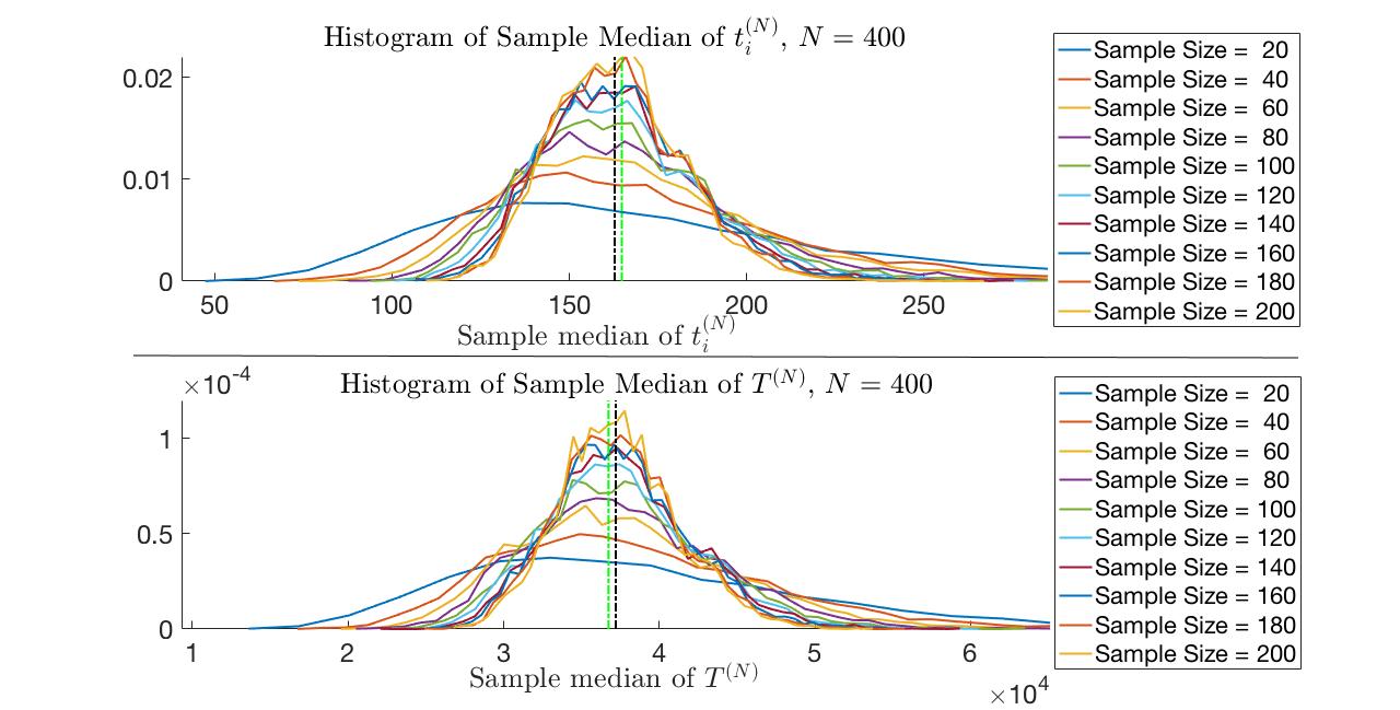
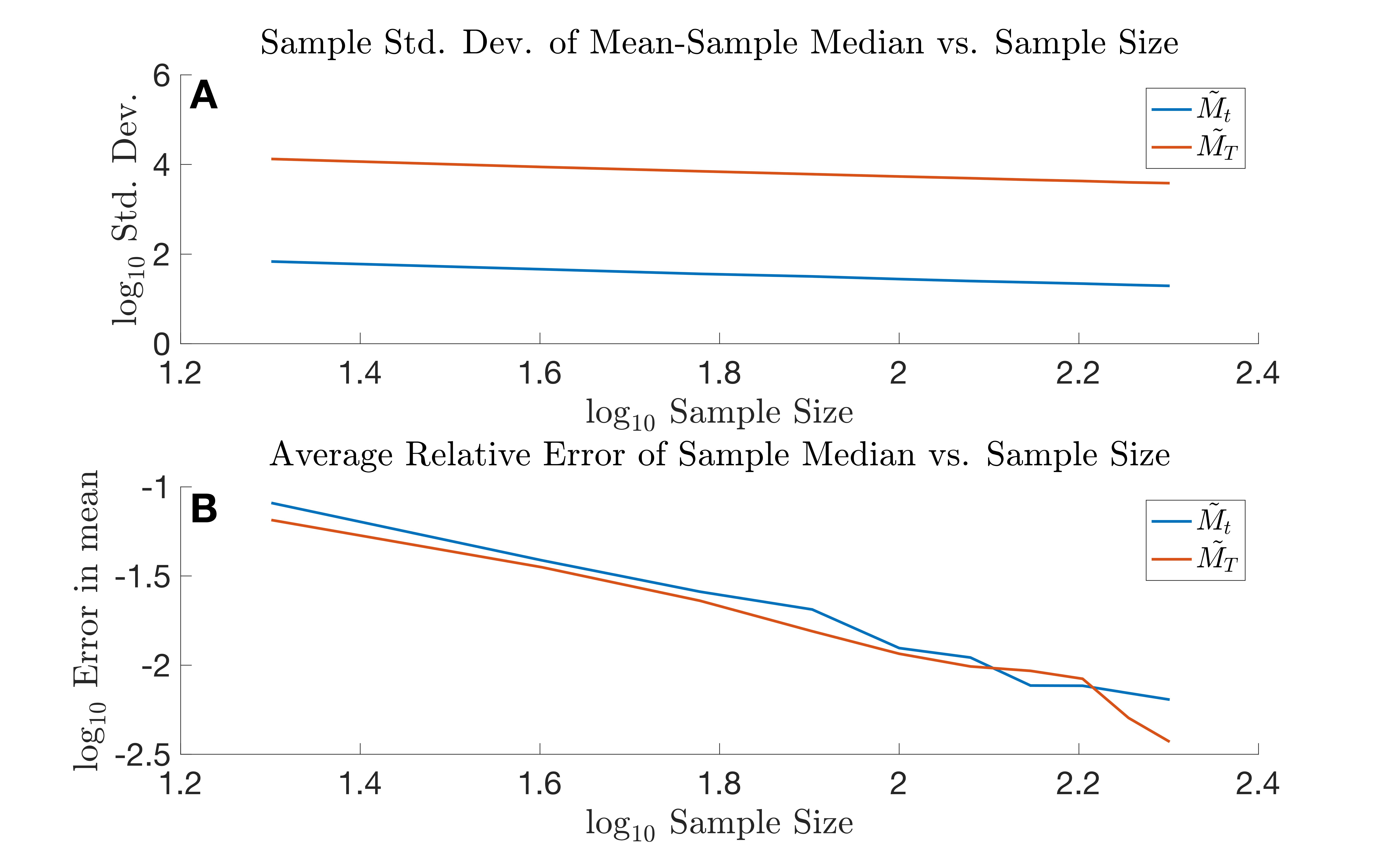
For a general random variable, $Y$, with density $f_{Y}$ and median $M_{Y}$, the sampling distribution of the sample median of $k$ iid samples from $Y$ converges to a normal distribution as the sample size approaches infinity. The mean of the normal distribution is $M_{Y}$ and its variance ${\color[rgb]{0,0,0}\definecolor[named]{pgfstrokecolor}{rgb}{0,0,0}\pgfsys@color@gray@stroke{0}\pgfsys@color@gray@fill{0}1/\big{(}}4k\,[f_{Y}(M_{Y})]^{2}{\color[rgb]{0,0,0}\definecolor[named]{pgfstrokecolor}{rgb}{0,0,0}\pgfsys@color@gray@stroke{0}\pgfsys@color@gray@fill{0}\big{)}}$ [8]. Histograms generated from sample medians under increasing sample sizes suggest this result extends to the sample median of both $t_{i}^{(N)}$ and $T^{(N)}$ (Fig. 5). Indeed, the $O(1/k)$ decay in the variance is observed across all particle numbers simulated. Additionally, if one uses the sample median of $10^{4}$ simulations as an approximation for the true medians, $M_{t}$ and $M_{T}$, then the mean of the sample medians converges to the true median at a rate which is $O(1/k)$ (Fig. 6). Specifically, for $k\geq 200$, the relative error between the mean sample median and the true median approximated from $10^{4}$ simulations was less than 1% for both $M_{t}$ and $M_{T}$ across all values of particle number simulated.

3.1 Median of $t_{i}^{(N)}$ under non-elastic collisions

We first present results on the behavior of the final collision time of a particle, $t_{i}^{(N)}.$ The median $M_{t}$ was approximated by selecting at random the final collision time of one particle from each of $10^{4}$ simulations and taking the median of these values. This process was repeated 100 times and the results were used to construct the 99% confidence intervals for the true median. This construction of the confidence intervals assumes the approximately normal distribution of the sample medians observed for elastic collisions persists under non-elastic collisions. We use $M_{t}^{elas}$ to denote the median final collision time under elastic collisions and $M_{t}^{inel}$ to denote the median final collision time under non-elastic collisions.

Before discussing the results, we propose an ansatz which relates path intersection times under elastic collisions to those under non-elastic collisions. Let $\epsilon=0$ and suppose that the path of particle 1 first intersects the path of particle 2, and then proceeds to intersect the path of particle 3. Let $\tau_{1,j}=\frac{X_{1}-X_{j}}{V_{j}-V_{1}}$, $j=2,3$ be the path intersection times between particle 1 and particles $j=2,3$, and let $\tau_{1,3}^{\prime}$ be the time at which the paths of particles 1 and 3 intersect under non-elastic collisions. If we assume particle 3 experiences a path intersection at approximately the same time that the paths of particles 1 and 2 coincide, then

$$\tau_{1,3}^{\prime}\approx\tau_{1,2}+\frac{(X_{1}+\tau_{1,2}V_{1})-(X_{3}+\tau_{1,2}V_{3})}{(1-\epsilon)(V_{3}-V_{1})}=\frac{1}{1-\epsilon}\tau_{1,3}.$$

Figure 7: The sample mean of the proportion of path intersections, $\overline{\alpha(\epsilon,N)},$ exhibits a clear dependence in $\epsilon N$, which is influenced by the initial velocity distribution.

Figure 8: Confidence intervals (95%) of the relative change in the median single particle final collision time. This quantity exhibits a clear dependence on $\epsilon N$, which is influenced by the velocity distribution. The coefficients of the regression $D_{1}(\epsilon N)+D_{2}(\epsilon N)^{2}$ applied to each of the four velocity distributions are displayed in Table 1.

Thus, under non-elastic collisions, the second path intersection time differs from the elastic path intersection time by a factor of $\frac{1}{1-\epsilon}.$ Generalizing this argument to the the $j^{th}$ interaction of particle 1,

$$\tau_{1,j}^{\prime}\approx\frac{1}{(1-\epsilon)^{j-1}}\tau_{1,j}.$$

This extension implicitly assumes that particle 1 has experienced an (approximately) equal number of path intersection as every other particle with which it interacts. Furthermore, the interactions should have occurred at approximately the same time. As such, it is not reasonable to expect the ansatz to apply to the longest intersection times, i.e. those which correspond to the final collision time of the system. However, assuming that one can extend this ansatz to the final collision time of a given particle, then non-elasticity alters $t_{i}^{(N)}$ by a multiplicative factor of the form

$$\frac{1}{(1-\epsilon)^{N\alpha(\epsilon,N)}}=e^{-\log(1-\epsilon){\color[rgb]{0,0,0}\definecolor[named]{pgfstrokecolor}{rgb}{0,0,0}\pgfsys@color@gray@stroke{0}\pgfsys@color@gray@fill{0}N}\alpha(\epsilon,N)}$$

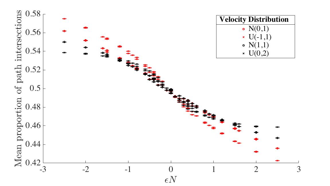
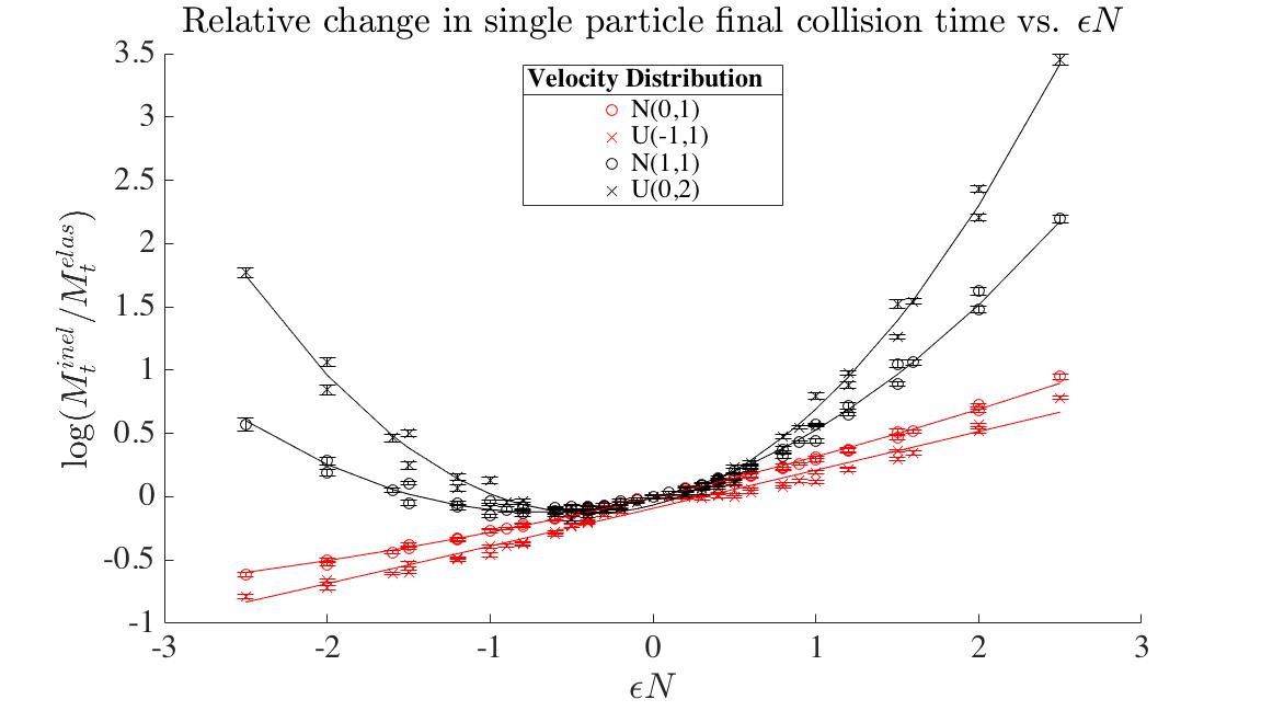
where $\alpha(\epsilon,N)$ represents the proportion of path intersections experienced by particle $i$. Since for $|\epsilon|\ll 1$, the multiplicative correction is approximately $\exp(\epsilon N\alpha(\epsilon,N))$, we expect $\log(M_{t}^{inel}{\color[rgb]{0,0,0}\definecolor[named]{pgfstrokecolor}{rgb}{0,0,0}\pgfsys@color@gray@stroke{0}\pgfsys@color@gray@fill{0}/}M_{t}^{elas})$ to depend on $\epsilon N$ at leading order. Furthermore, numerical simulations indicate that the mean proportion of path intersections, $\overline{\alpha(\epsilon,N)}$, is a function of $\epsilon N$ (Fig. 7), with leading order contribution equal to $1/2$. This is consistent with the sorting process interpretation of elastic collisions: each particle experiences $N-1$ path intersections, including both positive and negative times; given the symmetric distribution of $\tau_{i,j}$ about zero, half of these path intersections are expected to occur for $t>0$ on average. Therefore, one would expect $\log(M_{t}^{inel}/M_{t}^{elas})\sim\frac{\epsilon N}{2}$ at leading order. While the general structure of this relationship is correct, including the dependence on $\epsilon N$, a numerical reconstruction of $\log(M_{t}^{inel}/M_{t}^{elas})$ indicates this assumption is quantitatively inaccurate (Fig. 8). Indeed, applying a regression of the form $D_{1}(\epsilon N)+D_{2}(\epsilon N)^{2}$ to the median final collision results indicates that ${\color[rgb]{0,0,0}\definecolor[named]{pgfstrokecolor}{rgb}{0,0,0}\pgfsys@color@gray@stroke{0}\pgfsys@color@gray@fill{0}D_{1}}\approx 1/3$ rather than the value of $1/2$ predicted by the ansatz (Table 1). The difference is likely due to the assumption that particles experience equal path intersections, which is only reasonable for small times. A more rigorous study of the number of path intersections experienced by colliding particles could shed some light on this issue.

Distribution	$D_{1}$	$D_{2}$
$N(0,1)$	0.299364165261241	0.023741992291113
$U(-1,1)$	0.299564298338677	-0.0284407509187195
$N(1,1)$	0.315410496892726	0.221319632974651
$U(0,2)$	0.333999962446071	0.403837320001947

Table 1: Coefficients of the regression $D_{1}\epsilon N+D_{2}(\epsilon N)^{2}$ applied to $\log(M_{t}^{inel}/M_{t}^{elas})$. The linear term has a slope $D_{1}$ approximately equal to $1/3$ across all velocity distributions studied. The quadratic coefficient $D_{2}$ is much larger for the distributions centered about $1$.

This study highlights an important difference between elastic and non-elastic collisions. While the velocity distribution plays no role in determining the scaling of $t_{i}^{(N)}$ when $\epsilon=0$, it clearly affects the value of $C_{2}$ when $\epsilon\neq 0$, although the effect is weaker for those velocity distributions that are symmetric about zero.

3.2 Median of $T^{(N)}$ under non-elastic collisions

The median $M_{t}$ considered in the previous section captures the final collisions time of a randomly selected particle within the system, and therefore reflects the behavior of ‘typical’ particles. On the other hand, the final collision time of the system, $T^{(N)}$, arises from those particles that exhibit the largest final collision times, whose behavior is thus atypical. As such, the ansatz proposed in the previous section cannot be expected to adequately describe the behavior of $T^{(N)}$. Nonetheless, the numerical results of Fig. 9 confirm that $\log(M_{T}^{inel}/M_{T}^{elas})$ still depends on $\epsilon N$ and on the velocity distribution. Table 2 shows the coefficients obtained by applying a regression of the form $D_{1}(\epsilon N)+D_{2}(\epsilon N)^{2}$ to this quantity. As before, the effect on the quadratic term is stronger for distributions centered about $1$.

Distribution	$D_{1}$	$D_{2}$
$N(0,1)$	0.316098755619495	0.353122072713743
$U(-1,1)$	0.294877488559631	0.440060818253797
$N(1,1)$	0.270061962096432	1.65459638500048
$U(0,2)$	0.184011367253361	2.53476516441542

Table 2: Coefficients of the regression $D_{1}\epsilon N+D_{2}(\epsilon N)^{2}$ applied to $\log(M_{T}^{inel}/M_{T}^{elas})$. As in the study of $t_{i}^{(N)}$, the quadratic term is much larger for the distributions centered about $1$.

Figure 9: Confidence intervals for $\log(M_{T}^{inel}/M_{T}^{elas})$. The coefficients of the regression $D_{1}(\epsilon N)+D_{2}(\epsilon N)^{2}$ applied to each of the four velocity distributions are displayed in Table 2.

Figure 10: Confidence intervals for $\log(M_{T}^{inel}/NM_{t}^{elas})$ are symmetric about $\epsilon N=0.$ The coefficients of the regression $D_{0}+D_{1}(\epsilon N)+D_{2}(\epsilon N)^{2}$ applied to each of the four velocity distributions are displayed in Table 3.

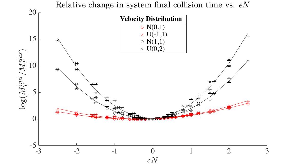
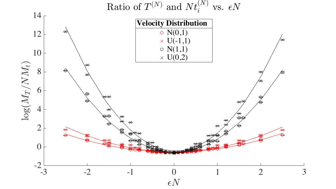
The asymmetry of $\log(M_{T}^{inel}/M_{T}^{elas})$ about $\epsilon N=0$ observed in Fig. 9 is due to the linear dependence of $t^{(N)}$ on $\epsilon N$. We checked that the ratio $M_{T}/NM_{t}$ behaves like $e^{O(1)+D_{2}(\epsilon N)^{2}}$(Figure 10 and Table 3). The $O(1)$ term arises from differences in the coefficients $C_{t}$ and $C_{T}$ that appear in the scaling of the medians, $M_{t}\sim{\color[rgb]{0,0,0}\definecolor[named]{pgfstrokecolor}{rgb}{0,0,0}\pgfsys@color@gray@stroke{0}\pgfsys@color@gray@fill{0}C}_{t}N$ and $M_{T}\sim C_{T}N^{2}$, under elastic collisions.

Distribution	$D_{0}$	$D_{1}$	$D_{2}$
$N(0,1)$	-0.542655411094044	0.0171180888904638	0.312943997391057
$U(-1,1)$	-0.517690994670863	-0.00466592391659517	0.424631130596750
$N(1,1)$	-0.512993538107585	-0.0466014260783037	1.40886890163564
$U(0,2)$	-0.419236799598809	-0.153106277504774	2.05627305470200

Table 3: Coefficients of the regression $D_{0}+D_{1}\epsilon N+D_{2}(\epsilon N)^{2}$ applied to $\log(M_{T}^{inel}/NM_{t}^{elas})$. The values of $C_{1}$ are much smaller than in the previous tables.

3.3 Discussion of Non-elastic Collisions

The rescaling of velocities by the factor $(1-\epsilon)>0$ each time a collision occurs results in an increase (decrease) in kinetic energy when $\epsilon<0$ ($\epsilon>0)$. While the overall increase (decrease) in the speed of particles is likely to increase (decrease) the rate at which collisions occur, surprisingly, the final collision times do not respond accordingly. For $|\epsilon N|\ll 1$, both $t_{i}^{(N)}$ and $T^{(N)}$ are decreasing functions of $\epsilon N$, consistent with the heating/cooling effects of the non-elastic collisions. However, as $|\epsilon N|$ moves away from zero, $T^{(N)}$ increases until it reaches values larger than that of elastic collisions. In the present simulations, this behavior is independent from the value, $0$ or $1$, of the average initial particle velocity. However, under non-elastic collisions, $t_{i}^{(N)}$ increases to values larger than that of elastic collisions only when the average initial velocity is $1$.

The numerical investigations discussed in this section lay out a possible path towards a rigorous construction of the asymptotic behavior of the final collision times by identifying three central questions: (i) does the proposed ansatz fail to accurately capture the effects of non-elastic collisions due to differences in path intersection counts and if so, to what extent? (ii) How do properties of the initial velocity distribution affect the scaling of the (median) collision times? And (iii), what aspects of the collision dynamics give rise to the observed increase in the median collision time? This last question is perhaps most difficult to answer for $T^{(N)}$, which is influenced largely by rare events (large collision times). We believe connections with the sorting processes outlined in Sections 1.1 and 1.2 may be able to offer some insight, although a preliminary numerical investigation (which is beyond the scope of this article) has proven inconclusive to this point.

4 Proofs of theorems

4.1 Proofs of Theorems Regarding $t_{i}^{(N)}$

We begin the proofs concerning Thms. 1 - 3 by deriving a formula for the exact distribution of $t_{i}^{(N)}=\max_{j\neq i}\tau_{i,j}$. Using independence of $\{(X_{i},V_{i})\}_{i=1}^{N}$ and by conditioning on the initial velocity and position of particle $i$, we can express the conditional probability of the event $\{t_{i}^{(N)}<\mu_{N}|(x_{i},v_{i})=(X,V)\}$ as follows.

$$\begin{split}P(t_{i}^{(N)}<\mu_{N}|(x_{i},v_{i})=(X,V))&=P(\tau_{i,1}<\mu_{N},\dots\color[rgb]{0,0,0}\definecolor[named]{pgfstrokecolor}{rgb}{0,0,0}\pgfsys@color@gray@stroke{0}\pgfsys@color@gray@fill{0},\tau_{i,i-1}<\mu_{N},\tau_{i,i+1}<\mu_{N}{\color[rgb]{0,0,0}\definecolor[named]{pgfstrokecolor}{rgb}{0,0,0}\pgfsys@color@gray@stroke{0}\pgfsys@color@gray@fill{0},}\dots\color[rgb]{0,0,0}\definecolor[named]{pgfstrokecolor}{rgb}{0,0,0}\pgfsys@color@gray@stroke{0}\pgfsys@color@gray@fill{0},\tau_{i,N}<\mu_{N}|(x_{i},v_{i})=(X,V))\\ &=[P(\tau_{i,1}<\mu_{N}|(x_{i},v_{i})=(X,V))]^{N-1}\\ &=\bigg{[}P\bigg{(}\frac{x_{1}-X}{V-v_{1}}<\mu_{N}\bigg{)}\bigg{]}^{N-1}.\end{split}$$ (5)

Integrating Eq. (5) with respect to the distribution of $(X,V)$ yields the unconditional probability of $\{t_{i}^{(N)}<\mu_{N}\}$,

$$\begin{split}P(t_{i}^{(N)}<\mu_{N})&=\int\int f_{x}(X)f_{v}(V)P(\tau_{i,j}<\mu_{N}|(x_{i},v_{i})=(X,V))dXdV\\ &=\int\int f_{x}(X)f_{v}(V)\bigg{[}P\bigg{(}\frac{x_{1}-X}{V-v_{1}}<\mu_{N}\bigg{)}\bigg{]}^{N-1}dXdV.\end{split}$$ (6)

Note that the integrand in Eq. (6) is dominated by $f_{x}(X)f_{v}(V)$. Thus, by dominated convergence, one can determine the asymptotic behavior $P(t_{i}^{(N)}<\mu_{N})$ by studying the large $N$ limit of Eq. (5). We search for a scaling of $\mu_{N}$ depending on $N$ such that

$$\bigg{[}P(t_{i}^{(N)}<\mu_{N}|(x_{i},v_{i})=(X,V))\bigg{]}^{N-1}=\bigg{[}P\bigg{(}\frac{x_{1}-X}{V-v_{1}}<\mu_{N}\bigg{)}\bigg{]}^{N-1}$$

has a non-trivial limit. We begin by constructing an integral representation of $\displaystyle P\bigg{(}\frac{x_{1}-X}{V-v_{1}}<\mu_{N}\bigg{)}$ by conditioning on the value of $v_{1}$.

$$\begin{split}P\bigg{(}\frac{x_{1}-X}{V-v_{1}}<\mu_{N}\bigg{)}&=P\bigg{(}x_{1}>X+(V-v_{1})\mu_{N},V<v_{i}\bigg{)}+P\bigg{(}x_{i}<X+(V-v_{1})\mu_{N},V\geq v_{i}\bigg{)}\\ &=\int_{V}^{\infty}\int_{X+\mu_{N}(V-v_{1})}^{\infty}f_{x}(x_{1})f_{v}(v_{1})dx_{1}dv_{1}+\int_{-\infty}^{V}\int_{-\infty}^{X+\mu_{N}(V-v_{1})}f_{v}(v_{1})f_{x}(x_{1})dx_{1}dv_{1}\\ &=\int_{V}^{\infty}f_{v}(v_{1})[1-F_{x}(X+\mu_{N}(V-v_{1})]dv_{1}+\int_{-\infty}^{V}f_{v}(v_{1})F_{X}(X+\mu_{N}(V-v_{1}))dv_{1}\end{split}$$ (7)

Applying the change of variables $w=v_{1}-V$ gives a more useful representation of Eq. (7).

$$\begin{split}P\bigg{(}\frac{x_{1}-X}{V-v_{1}}<\mu_{N}\bigg{)}&=\int_{0}^{\infty}f_{v}(w+V)[1-F_{x}(X-\mu_{N}w)]dw+\int_{-\infty}^{0}f_{v}(w+V)F_{x}(X-\mu_{N}w)dw\\ &=1-\int_{0}^{\infty}f_{v}(w+V)F_{x}(X-\mu_{N}w)dw-\int_{-\infty}^{0}f_{v}(w+V)[1-F_{x}(X-\mu_{N}w)]dw\end{split}$$ (8)

Inputting the result from Eq. (8) in Eq. (6) gives an integral representation of the distribution of $t_{i}^{(N)}.$

$$\begin{split}P(t_{i}^{(N)}<\mu_{N})&=\int_{\mathbb{R}^{2}}f_{x}(X)f_{v}(V)\bigg{[}1-\int_{0}^{\infty}f_{v}(w+V)F_{x}(X-\mu_{N}w)dw\\ &\hskip 113.81102pt-\int_{-\infty}^{0}f_{v}(w+V)[1-F_{x}(X-\mu_{N}w)]dw\bigg{]}^{N-1}dXdV\end{split}$$ (9)

The results of Thms. 1 - 3 depend on the pointwise limit of

$$g(X,V,N)=\bigg{[}1-\int_{0}^{\infty}f_{v}(w+V)F_{x}(X-\mu_{N}w)dw-\int_{-\infty}^{0}f_{v}(w+V)[1-F_{x}(X-\mu_{N}w)]dw\bigg{]}^{N-1}$$ (10)

as $N\to\infty$ under a suitable choice of $\mu_{N}.$ In particular, as $g(X,V,N)$ is a probability, hence bounded by one, we have the following proposition.

Proposition 3.

Suppose that $\lim_{N\to\infty}g(X,V,N)$ exists. Then,

$$\begin{split}\lim_{N\to\infty}P\bigg{(}t_{i}^{(N)}<\mu_{N}\bigg{)}&=\lim_{N\to\infty}\int_{\mathbb{R}^{2}}f_{x}(X)f_{v}(V)g(X,V,N)dXdV=\int_{\mathbb{R}^{2}}f_{x}(X)f_{v}(V)\bigg{(}\lim_{N\to\infty}g(X,V,N)\bigg{)}dXdV\end{split}$$ (11)

The details of the proofs of Thms.1 - 3 consider the pointwise limit of $g(X,V,N)$ as $N\to\infty.$ Since the proof of Theorem 3 is similar to that of Theorem 2, we have placed it in the appendix.

Proof of Theorem 1.

Suppose that $E|X_{1}|<\infty$ and $f_{v}$ is continuous and bounded. Let $\mu_{N}=\mu N$ with $\mu>0.$ Consider the pointwise limit of $g(X,V,N)$ as $N\to\infty.$

$$\begin{split}g(X,V,N)&=\bigg{[}1-\int_{0}^{\infty}f_{v}(w+V)F_{x}(X-\mu Nw)dw-\int_{-\infty}^{0}f_{v}(w+V)[1-F_{x}(X-\mu Nw)]dw\bigg{]}^{N-1}\\ &=\bigg{[}1-\frac{1}{N}\int_{0}^{\infty}f_{v}(w/N+V)F_{x}(X-\mu w)dw-\frac{1}{N}\int_{-\infty}^{0}f_{v}(w/N+V)[1-F_{x}(X-\mu w)]dw\bigg{]}^{N-1}\\ &=\exp\bigg{\{}(N-1)\ln\bigg{(}1-\frac{1}{N}\int_{0}^{\infty}f_{v}(w/N+V)F_{x}(X-\mu w)dw\\ &\hskip 142.26378pt-\frac{1}{N}\int_{-\infty}^{0}f_{v}(w/N+V)[1-F_{x}(X-\mu w)]dw\bigg{)}\bigg{\}}\end{split}$$ (12)

Recall that $E|X|<\infty$, so both $\displaystyle\int_{0}^{\infty}F_{x}(X-\mu w)dw$ and $\displaystyle\int_{-\infty}^{0}[1-F_{x}(X-\mu w)]dw$ are finite. Additionally,

$$\begin{split}0&<f_{v}(w/N+V)F_{x}(X-\mu w)\leq M_{v}F_{x}(X-\mu w)\\ 0&<f_{v}(w/N+V)[1-F_{x}(X-\mu w)]<M_{v}[1-F_{x}(X-\mu w)]\\ \end{split}$$

where $M_{v}=\sup|f_{v}|$. By dominated convergence, it follows that

$$\begin{split}\lim_{N\to\infty}\int_{0}^{\infty}f_{v}(w/N+V)F_{x}(X-\mu w)dw&=\int_{\mathbb{R}}f_{v}(V)F_{x}(X-\mu w)dw\\ \lim_{N\to\infty}\int_{-\infty}^{0}f_{v}(w/N+V)[1-F_{x}(X-\mu w)]dw&=\int_{-\infty}^{0}f_{v}(V)[1-F_{x}(X-\mu w)]dw\end{split}$$

Hence, by the relation $\ln(1-x)=-x+o(x)$ for small $x$, then as $N$ tends to $\infty$,

$$\begin{split}g(X,V,N)&=\exp\bigg{\{}-\frac{N-1}{N}\bigg{(}\int_{0}^{\infty}f_{v}(V)F_{x}(X-\mu w)dw+\int_{-\infty}^{0}f_{v}(V)[1-F_{x}(X-\mu w)]\bigg{)}+o(1)\bigg{\}}\\ &\to\exp\bigg{\{}-f_{v}(V)\bigg{(}\int_{0}^{\infty}F_{x}(X-\mu w)dw+\int_{-\infty}^{0}[1-F_{x}(X-\mu w)]dw\bigg{)}\bigg{\}}.\\ \end{split}$$ (13)

Furthermore,

$$\begin{split}&\int_{0}^{\infty}F_{x}(X-\mu w)dw+\int_{-\infty}^{0}[1-F_{x}(X-\mu w)]dw=\frac{1}{\mu}\int_{0}^{\infty}F_{x}(X-y)dy+\frac{1}{\mu}\int_{-\infty}^{0}[1-F_{x}(X-y)]dy\\ &=\frac{1}{\mu}\bigg{(}\int_{0}^{\infty}yf_{x}(X-y)dy-\int_{-\infty}^{0}yf_{x}(X-y)dy\bigg{)}=\frac{1}{\mu}\bigg{(}\int_{-\infty}^{X}(X-y)f_{x}(y)dy-\int_{X}^{\infty}(X-y)f_{x}(y)dy\bigg{)}\\ &=\frac{1}{\mu}\int_{\mathbb{R}}|X-y|f_{x}(y)dy\end{split}$$ (14)

So that for $\mu>0$, $\mu_{N}=\mu\cdot N$, and with the representation of $P(\frac{t_{i}^{(N)}}{N}\leq\mu)$ from Eq. (11), we have the desired result:

$$\lim_{N\to\infty}g(X,V,N)=\exp\bigg{\{}-\frac{1}{\mu}f_{v}(V)\int_{\mathbb{R}}|X-y|f_{x}(y)dy\bigg{\}}.$$

Thus, by Proposition 3,

$$\lim_{N\to\infty}P\bigg{(}\frac{t_{i}^{(N)}}{N}<\mu\bigg{)}=\int_{\mathbb{R}^{2}}f_{x}(X)f_{v}(V)\exp\bigg{\{}-\frac{1}{\mu}f_{v}(V)\int_{\mathbb{R}}|X-y|f_{x}(y)dy\bigg{\}}dXdV.$$

∎

Proof of Theorem 2.

As in the proof of Thm. 1, we proceed by investigating the large $N$ behavior of $g(X,V,N)$. However, unlike Thm. 1, we assume that $\{X_{i}\}_{i=1}^{N}$ have density $f_{x}(x)=\frac{C_{\alpha}}{1+|x|^{1+\alpha}}$ for $0<\alpha<1$, so that $E|X_{i}|=\infty$ and

$$\int_{0}^{\infty}F_{x}(X-w)dw=\int_{-\infty}^{0}[1-F_{x}(X-w)]dw=\infty.$$

Now for $\mu>0$, we take $\mu_{N}=\mu\cdot N^{1/\alpha}$ and begin with the form of $g(X,V,N)$ from Eq. (10).

$$\begin{split}g(X,V,N)&=\bigg{[}1-\int_{0}^{N^{\alpha-2}}f_{v}(w+V)F_{x}(X-\mu N^{1/\alpha}w)dw-\int_{-{N^{\alpha-2}}}^{0}f_{v}(w+V)[1-F_{x}(X-\mu N^{1/\alpha}w)]dw\\ &\hskip 17.07182pt-\int_{{N^{\alpha-2}}}^{\infty}f_{v}(w+V)F_{x}(X-\mu N^{1/\alpha}w)dw-\int_{-\infty}^{-{N^{\alpha-2}}}f_{v}(w+V)[1-F_{x}(X-\mu N^{1/\alpha}w)]dw\bigg{]}^{N-1}\end{split}$$ (15)

We now investigate the large $N$ behavior of the different integrals within Eq. (15). The following statements follow from the boundedness of $f_{v}$. For fixed $(X,V)$,

$$\begin{split}\int_{0}^{{N^{\alpha-2}}}f_{v}(w+V)F_{x}(X-\mu N^{1/\alpha}w)dw&=O(1)N^{\alpha-2}=o\bigg{(}\frac{1}{N}\bigg{)}\\ \int_{-{N^{\alpha-2}}}^{0}f_{v}(w+V)[1-F_{x}(X-\mu N^{1/\alpha}w)]dw&=O(1){N^{\alpha-2}}=o\bigg{(}\frac{1}{N}\bigg{)}\end{split}$$

For the remaining integrals in $g(X,V,N)$, we need some bounds on $F_{x}(-z)$ and $1-F_{x}(z)$ for large $z$. Note that,

$$F_{x}(-z)=\int_{-\infty}^{-z}\frac{C_{\alpha}}{1+|t|^{1+\alpha}}dt=C_{\alpha}\int_{-\infty}^{-z}\frac{1}{|t|^{1+\alpha}}\frac{1}{1+\frac{1}{|t|^{1+\alpha}}}dt\\$$ (16)

Thus, by the symmetry of $f_{x}$ we have the following bounds of $F_{x}(-z)=1-F_{x}(z)$

$$\frac{1}{1+\frac{1}{|z|^{1+\alpha}}}\frac{C_{\alpha}}{\alpha}|z|^{-\alpha}=\frac{C_{\alpha}}{1+\frac{1}{|z|^{1+\alpha}}}\int_{-\infty}^{-z}\frac{1}{|t|^{1+\alpha}}dt\leq F_{x}(-z)=1-F_{x}(z)\leq C_{\alpha}\int_{-\infty}^{-z}\frac{1}{|t|^{1+\alpha}}dt=\frac{C_{\alpha}}{\alpha}|z|^{-\alpha}.$$ (17)

The upper and lower bounds converge as $z\to\infty$ so we have the following scaling laws for large $z$,

$$F_{x}(-z)=1-F_{x}(z)=\frac{C_{\alpha}}{\alpha}|z|^{-\alpha}+O\bigg{(}\frac{1}{|z|^{1+2\alpha}}\bigg{)}\\$$ (18)

Note that $N^{\alpha-2}\cdot N^{1/\alpha}=N^{(1-\alpha)^{2}/\alpha}.$ Thus, we can take $N$ large, depending on $\mu$ and $X$, so that $\mu N^{1/\alpha}w-X\geq\mu N^{(1-\alpha)^{2}/\alpha}-X>>1$ for all $w\geq N^{\alpha-2}$ allowing us to make use of the bounds from Eq. (17) in the remaining integrals in $g(X,V,N).$ Then, for fixed $(X,V)$,

$$\int_{N^{\alpha-2}}^{\infty}f_{v}(w+V)F_{x}(X-\mu N^{1/\alpha}w)dw=\int_{N^{\alpha-2}}^{\infty}f_{v}(w+V)\bigg{(}\frac{C_{\alpha}}{\alpha}\frac{1}{|X-\mu N^{1/\alpha}w|^{\alpha}}+O\bigg{(}\frac{1}{|X-\mu N^{1/\alpha}w|^{1+2\alpha}}\bigg{)}\bigg{)}dw\\$$ (19)

Recall that $f_{v}$ is bounded. Let $M_{v}=\sup|f_{v}|$. We observe that the correction in the preceding integral is $o(1/N)$ as follows.

$$\begin{split}\int_{N^{\alpha-2}}^{\infty}\frac{f_{v}(w+V)}{|X-\mu N^{1/\alpha}w|^{1+2\alpha}}dw&\leq\int_{N^{\alpha-2}}^{\infty}\frac{M_{v}}{|X-\mu N^{1/\alpha}w|^{1+2\alpha}}dw\\ &=\frac{M_{v}}{2\alpha\mu N^{1/\alpha}}\cdot\frac{1}{|\mu N^{(1-\alpha)^{2}/\alpha}-X|^{2\alpha}}=O\bigg{(}\frac{1}{N^{1/\alpha+2(1-\alpha)^{2}}}\bigg{)}\end{split}$$ (20)

The quantity $2(1-\alpha)^{2}\geq 0$. Therefore, $\alpha\in(0,1)$ implies $1/\alpha+2(1-\alpha)^{2}>1$. Hence,

$$\begin{split}\int_{N^{\alpha-2}}^{\infty}f_{v}(w+V)F_{x}(X-\mu N^{1/\alpha}w)dw&=\frac{1}{N}\frac{C_{\alpha}}{\alpha\mu^{\alpha}}\int_{N^{\alpha-2}}^{\infty}f_{v}(w+V)\frac{1}{w^{\alpha}}\frac{1}{|X/(\mu wN^{1/\alpha})-1|^{\alpha}}dw+o\bigg{(}\frac{1}{N}\bigg{)}\\ &=\frac{1}{N}\frac{C_{\alpha}}{\alpha\mu^{\alpha}}\int_{0}^{\infty}\frac{f_{v}(w+V)}{w^{\alpha}}dw+o\bigg{(}\frac{1}{N}\bigg{)}\end{split}$$ (21)

Finally, for the final integral in Eq. (15). We make the following change of variables.

$$\int_{-\infty}^{-{N^{\alpha-2}}}f_{v}(w+V)[1-F_{x}(X-\mu N^{1/\alpha}w)]dw=\int_{N^{\alpha-2}}^{\infty}f_{v}(V-w)[1-F_{x}(X+\mu N^{1/\alpha}w)]dw.$$

To which we apply the same arguments as above to show

$$\int_{-\infty}^{-{N^{\alpha-2}}}f_{v}(w+V)[1-F_{x}(X-\mu N^{1/\alpha}w)]dw=\frac{C_{\alpha}}{\alpha\mu^{\alpha}N}\int_{0}^{\infty}{\color[rgb]{0,0,0}\definecolor[named]{pgfstrokecolor}{rgb}{0,0,0}\pgfsys@color@gray@stroke{0}\pgfsys@color@gray@fill{0}\frac{f_{v}(V-w)}{w^{\alpha}}}dw+o\bigg{(}\frac{1}{N}\bigg{)}$$

Thus,

$$\begin{split}&\lim_{N\to\infty}g(X,V,N)={\color[rgb]{0,0,0}\definecolor[named]{pgfstrokecolor}{rgb}{0,0,0}\pgfsys@color@gray@stroke{0}\pgfsys@color@gray@fill{0}\lim_{N\to\infty}}\bigg{(}1-\frac{C_{\alpha}}{\alpha\mu^{\alpha}N}\int_{0}^{\infty}\frac{f_{v}(V+w)+f_{v}(V-w)}{w^{\alpha}}dw+o(1/N)\bigg{)}^{N-1}\\ &=\exp\bigg{\{}-\frac{C_{\alpha}}{\alpha\mu^{\alpha}}\int_{0}^{\infty}\frac{f_{v}(V+w)+f_{v}(V-w)}{w^{\alpha}}dw\bigg{\}}=\exp\bigg{\{}-\frac{C_{\alpha}}{\alpha\mu^{\alpha}}\int_{-\infty}^{\infty}\frac{f_{v}(V+w)}{|w|^{\alpha}}dw\bigg{\}}\end{split}$$ (22)

which in turns gives the desired result.

$$\lim_{N\to\infty}P\bigg{(}\frac{t_{i}^{(N)}}{N^{1/\alpha}}<\mu\bigg{)}=\int_{\mathbb{R}^{2}}f_{x}(X)f_{v}(V)\exp\bigg{(}-\frac{C(V)}{\mu^{\alpha}}\bigg{)}dXdV$$

where

$$C(V)=\frac{C_{\alpha}}{\alpha}\int_{\mathbb{R}}f_{v}(V+w)\frac{1}{|w|^{\alpha}}dw.$$

∎

4.2 Proofs of Theorems Regarding $T^{(N)}$

The key observation in the proofs of Theorems 4, 5, and 6 and Propositions 2 is that for any time $z_{N}(t)\in\mathbb{R}$, the final collision time $T^{(N)}$ does not exceed $z_{N}(t)$ if and only if the random variable $A_{N,z_{N}(t)}=\sum_{1\leq i<j\leq N}\mathbf{1}_{\tau_{i,j}>z_{N}(t)}$ does not exceed one. The distribution of $A_{N,z_{N}(t)}$ can be approximated by a Poisson distribution [11, 14, 5]. We state Corollary 2.1 from [11].

Silverman-Brown Limit Law [11].

Let $\xi_{1},\dots,\xi_{N}$ be $\mathbb{S}$-valued random variables and $h:\mathbb{S}^{k}\to\mathbb{R}$ be a symmetric Borel function. Let

$$\begin{split}p_{N,z}&=P(h(\xi_{1},\dots,\xi_{k})>z),\\ \lambda_{N,z}&=\binom{N}{k}p_{N,z}\end{split}$$

If for some sequence of transformations, $z_{N}:\mathbb{T}\to\mathbb{R}$ with $\mathbb{T}\subset\mathbb{R}$, the conditions

$$\lim_{N\to\infty}\lambda_{N,z_{N}(t)}=\lambda_{t}>0$$

and

$$\lim_{N\to\infty}N^{2k-1}P\bigg{(}h(\xi_{1},\dots,{\color[rgb]{0,0,0}\definecolor[named]{pgfstrokecolor}{rgb}{0,0,0}\pgfsys@color@gray@stroke{0}\pgfsys@color@gray@fill{0}\xi_{k}})>z_{N}(t),h(\xi_{1+k-r},\dots,\xi_{2k-r})>z_{N}(t)\bigg{)}={\color[rgb]{0,0,0}\definecolor[named]{pgfstrokecolor}{rgb}{0,0,0}\pgfsys@color@gray@stroke{0}\pgfsys@color@gray@fill{0}0}$$

hold for all $t\in\mathbb{T}$ and $r=1,2,\dots,k-1$, then

$$\lim_{N\to\infty}P(H_{N}\leq z_{N}(t))=\exp(-\lambda_{t})$$

for all $t\in\mathbb{T}$ where $H_{N}=\max\limits_{1\leq j_{1}\leq\dots\leq j_{k}\leq N}h(\xi_{j_{1}},\dots,\xi_{j_{k}}).$

Returning to our problem, let $\xi_{i}=(X_{i},V_{i})$ be the initial position and velocity of particle $i$ and $h:\mathbb{S}^{2}\to\mathbb{R}$ be the function which gives the path intersection time of two particles

$$h(\xi_{i},\xi_{j})=h\bigg{(}(X_{i},V_{i}),(X_{j},V_{j})\bigg{)}=\frac{X_{i}-X_{j}}{V_{j}-V_{i}}=\tau_{i,j}.$$

Then $H_{N}$ from the Silverman-Brown Limit Law stated above is the maximum collision time of the system, $T^{(N)}$. To prove Theorems 4, 5, and 6, we need to find a time scale $z_{N}(t)$ such that

$$\binom{N}{2}P(\tau_{1,2}>z_{N}(t)) \to\lambda_{t}>0$$ (23)

$$N^{3}P(\tau_{1,2}>z_{N}(t),\tau_{2,3}>z_{N}(t)) \to 0.$$ (24)

The random variable $A_{N,z_{N}(t)}$ previously introduced is a summation of the $\binom{N}{2}$ dependent, Bernoulli random variables, $\mathbf{1}_{\tau_{i,j}>z_{N}(t)}$. Recounting the idea of the proof of the Silverman-Brown law, when Eq. (24) is satisfied, these random variable become sufficiently uncorrelated as $N\to\infty$ so that the distribution of $A_{N,z_{N}(t)}$ is approximately $Bin(\binom{N}{2},p_{N,z_{N}(t)})$. The choice of $z_{N}(t)$ which gives a non-trivial limit in Eq. (23) allows one to approximate the distribution of $A_{N,z_{N}(t)}$ as $Poisson(\lambda_{t})$. We mention that detailed error bounds for the Poisson approximation can be found in [5].

Proof of Theorem 4.

Let $z_{N}(t)=\binom{N}{2}t$ and consider the behavior of $\lambda_{N,z_{N}(t)}$ as $N\to\infty.$

$$\begin{split}\lambda_{N,z_{N}(t)}&=\binom{N}{2}P(\tau_{1,2}>z_{N}(t))=\binom{N}{2}\bigg{(}1-P(\tau_{1,2}\leq z_{N}(t))\bigg{)}\\ &=\binom{N}{2}\bigg{(}\int_{\mathbb{R}^{2}}\int_{0}^{\infty}f_{x}(X)f_{v}(V)f_{v}(w+V)F_{x}(X-z_{N}(t)w)dwdXdV\\ &\hskip 71.13188pt+\int_{\mathbb{R}^{2}}\int_{-\infty}^{0}f_{x}(X)f_{v}(V)f_{v}(w+V)(1-F_{x}(X-z_{N}(t)w))dwdXdV\bigg{)}\end{split}$$ (25)

where the last equality follows from Eq. (9) taking $N=2$ and noting that $t_{1}^{(2)}=\tau_{1,2}$ ( recall that ${\color[rgb]{0,0,0}\definecolor[named]{pgfstrokecolor}{rgb}{0,0,0}\pgfsys@color@gray@stroke{0}\pgfsys@color@gray@fill{0}t_{1}^{(2)}}$ is the (first and) last collision time in a system of two particles). Making use of the change of variable $y=\binom{N}{2}w$ we have the following representation for $\lambda_{N,z_{N}(t)}$

$$\begin{split}\lambda_{N,z_{N}(t)}&=\int_{\mathbb{R}^{2}}\int_{0}^{\infty}f_{x}(X)f_{v}(V)f_{v}\bigg{(}V+\frac{y}{\binom{N}{2}}\bigg{)}F_{x}(X-ty)dydXdV\\ &\hskip 56.9055pt+\int_{\mathbb{R}^{2}}\int_{-\infty}^{0}f_{x}(X)f_{v}(V)f_{v}\bigg{(}V+\frac{y}{\binom{N}{2}}\bigg{)}(1-F_{x}(X-ty))dydXdV\end{split}$$ (26)

Under the assumption that $f_{v}$ is bounded and $E|X_{1}|<\infty$, we can evaluate $\lim_{N\to\infty}\lambda_{N,z_{N}(t)}$ by use of the dominated convergence theorem.

$$\begin{split}\lim_{N\to\infty}\lambda_{N,z_{N}(t)}&=\int_{\mathbb{R}^{2}}\int_{0}^{\infty}f_{x}(X)(f_{v}(V))^{2}F_{x}(X-ty)dydXdV\\ &\hskip 56.9055pt+\int_{\mathbb{R}^{2}}\int_{-\infty}^{0}f_{x}(X)(f_{v}(V))^{2}(1-F_{x}(X-ty))dydXdV\\ &=\bigg{(}\int_{-\infty}^{\infty}f_{v}^{2}(V)dV\bigg{)}\int_{-\infty}^{\infty}f_{x}(X)\bigg{(}\int_{0}^{\infty}F_{x}(X-ty)dy+\int_{-\infty}^{0}(1-F_{x}(X-ty))dy\bigg{)}dX\\ &=\frac{1}{t}\int_{-\infty}^{\infty}f_{v}^{2}(V)dV\cdot\int_{\mathbb{R}^{2}}|X-y|f_{x}(X)f_{x}(y)dydX\end{split}$$ (27)

where the last equality follows from the same argument as in Eq. (14). We have now determined the appropriate scaling to use in the Silverman-Brown limit law. All that remains to be shown is that

$$N^{3}P(\tau_{1,2}>z_{N}(t),\tau_{2,3}>z_{N}(t))\to 0$$

as $N\to\infty.$ To prove this limit we first note the event $\{\tau_{1,2}>z_{N}(t),\tau_{2,3}>z_{N}(t)\}$ is equivalent to the event $\{t_{2}^{(3)}>z_{N}(t)\}$. We can construct an integral representation for $P(t_{2}^{(3)}>z_{N}(t))$ following a similar argument used in the construction of Eq. (9).

$$\begin{split}&N^{3}P(\tau_{1,2}>z_{N}(t),\tau_{2,3}>z_{N}(t))\\ =\ &N^{3}\int_{\mathbb{R}^{2}}f_{x}(X)f_{v}(V)P\bigg{(}\frac{x_{1}-X}{V-v_{1}}>z_{N}(t),\frac{x_{3}-X}{V-v_{3}}{\color[rgb]{0,0,0}\definecolor[named]{pgfstrokecolor}{rgb}{0,0,0}\pgfsys@color@gray@stroke{0}\pgfsys@color@gray@fill{0}>z_{N}(t)}\bigg{|}(x_{2},v_{2})=(X,V)\bigg{)}dXdV\\ =\ &N^{3}\int_{\mathbb{R}^{2}}f_{x}(X)f_{v}(V)\bigg{[}P\bigg{(}\frac{x_{1}-X}{V-v_{1}}>z_{N}(t)\bigg{)}\bigg{]}^{2}dXdV\end{split}$$ (28)

From Eq. (8), it follows that

$$P\bigg{(}\frac{x_{1}-X}{V-v_{1}}>z_{N}(t)\bigg{)} =1-P\bigg{(}\frac{x_{1}-X}{V-v_{1}}\leq z_{N}(t)\bigg{)}$$

$$=\int_{0}^{\infty}f_{v}(w+V)F_{x}(X-z_{N}(t)w)dw+\int_{-\infty}^{0}f_{v}(w+V)(1-F_{x}(X-z_{N}(t)w))dw$$

Substituting the above equality into Eq. (28), we continue the calculation.

$$\begin{split}&N^{3}P(\tau_{1,2}>z_{N}(t),\tau_{2,3}>z_{N}(t))\\ &=N^{3}\int_{\mathbb{R}^{2}}f_{x}(X)f_{v}(V)\bigg{(}\int_{0}^{\infty}f_{v}(w+V)F_{x}(X-z_{N}(t)w)dw+\int_{-\infty}^{0}f_{v}(w+V)(1-F_{x}(X-z_{N}(t)w))dw\bigg{)}^{2}dXdV\\ &=N^{3}\int_{\mathbb{R}^{2}}f_{x}(X)f_{v}(V)\bigg{(}\int_{0}^{\infty}f_{v}(w+V)P(X^{\prime}\leq X-z_{N}(t)w)dw+\int_{0}^{\infty}f_{v}(V-w)P(X^{\prime}>X+z_{N}(t)w)dw\bigg{)}^{2}dXdV\end{split}$$ (29)

where $X^{\prime}$ has the same distribution as $X_{1}$. We now make use of the assumption that $E|X_{1}|^{3/2}<\infty$ . Also, recall $z_{N}(t)=\binom{N}{2}t.$

$$\begin{split}&N^{3}P(\tau_{1,2}>z_{N}(t),\tau_{2,3}>z_{N}(t))\\ &\leq N^{3}\int_{\mathbb{R}^{2}}f_{x}(X)f_{v}(V)\bigg{(}\int_{0}^{\infty}f_{v}(w+V)P(|X-X^{\prime}|\geq z_{N}(t)w)dw\\ &\hskip 113.81102pt+\int_{0}^{\infty}f_{v}(V-w)P(|X^{\prime}-X|>z_{N}(t)w)dw\bigg{)}^{2}dXdV\\ &=N^{3}\int_{\mathbb{R}^{2}}f_{x}(X)f_{v}(V)\bigg{(}\int_{0}^{\infty}[f_{v}(V-w)+f_{v}(V+w)]P(|X^{\prime}-X|\geq z_{N}(t)w)dw\bigg{)}^{2}dXdV\\ &\leq N^{3}\int_{\mathbb{R}^{2}}f_{x}(X)f_{v}(V)\bigg{(}\int_{0}^{\infty}[f_{v}(V-w)+f_{v}(V+w)]\frac{E_{X^{\prime}}(|X^{\prime}-X|^{3/4}\mathbbm{1}_{|X^{\prime}-X|>z_{N}(t)w})}{(z_{N}(t)w)^{3/4}}dw\bigg{)}^{2}dXdV\\ &=C_{N}(t)\int_{\mathbb{R}^{2}}f_{x}(X)f_{v}(V)\bigg{(}\int_{0}^{\infty}\frac{f_{v}(V-w)+f_{v}(V+w)}{w^{3/4}}E_{X^{\prime}}(|X^{\prime}-X|^{3/4}\mathbbm{1}_{|X^{\prime}-X|>z_{N}(t)w}){\color[rgb]{0,0,0}\definecolor[named]{pgfstrokecolor}{rgb}{0,0,0}\pgfsys@color@gray@stroke{0}\pgfsys@color@gray@fill{0}dw}\bigg{)}^{2}dXdV\end{split}$$ (30)

where $E_{X^{\prime}}[\cdot]$ is expectation with respect to $X^{\prime}$ and $C_{N}(t)=\frac{N^{3}}{(N^{2}-N)^{3/2}}\frac{2^{3/2}}{t^{3/2}}\to\big{(}\frac{2}{t}\big{)}^{3/2}$ as $N\to\infty.$ Thus, to show $N^{3}P(\tau_{1,2}>z_{N}(t),\tau_{2,3}>z_{N}(t))\to 0$ as $N\to\infty$, we need to show the final integral in Eq. (30) approaches zero as $N\to\infty.$ The integrand can be dominated as follows.

$$\begin{split}&f_{x}(X)f_{v}(V)\bigg{(}\int_{0}^{\infty}\frac{f_{v}(V-w)+f_{v}(V+w)}{w^{3/4}}E_{X^{\prime}}(|X^{\prime}-X|^{3/4}\mathbbm{1}_{|X^{\prime}-X|>z_{N}(t)w}){\color[rgb]{0,0,0}\definecolor[named]{pgfstrokecolor}{rgb}{0,0,0}\pgfsys@color@gray@stroke{0}\pgfsys@color@gray@fill{0}dw}\bigg{)}^{2}\\ &\leq f_{x}(X)f_{v}(V)\bigg{(}\int_{0}^{\infty}\frac{f_{v}(V-w)+f_{v}(V+w)}{w^{3/4}}dw\bigg{)}^{2}\bigg{(}E_{X^{\prime}}(|X^{\prime}-X|^{3/4})\bigg{)}^{2}\\ &\leq f_{x}(X)f_{v}(V)\bigg{(}\int_{1}^{\infty}(f_{v}(V-w)+f_{v}(V+w)){\color[rgb]{0,0,0}\definecolor[named]{pgfstrokecolor}{rgb}{0,0,0}\pgfsys@color@gray@stroke{0}\pgfsys@color@gray@fill{0}dw}+\int_{0}^{1}\frac{2M_{v}}{w^{3/4}}dw\bigg{)}^{2}E_{X^{\prime}}|X^{\prime}-X|^{3/2}\\ &\leq f_{x}(X)f_{v}(V)(1+8M_{v})^{2}E_{X^{\prime}}(|X^{\prime}|+|X|)^{3/2}\end{split}$$ (31)

where $M_{v}=\max\limits_{y}f_{v}(y).$ The final equation in Eq. (31) is integrable since $X_{1}$ has a 3/2 moment. Using dominated convergence twice,

$$\begin{split}&\lim_{N\to\infty}\int_{\mathbb{R}^{2}}f_{x}(X)f_{v}(V)\bigg{(}\int_{0}^{\infty}\frac{f_{v}(V-w)+f_{v}(V+w)}{w^{3/4}}E_{X^{\prime}}(|X^{\prime}-X|^{3/4}\mathbbm{1}_{|X^{\prime}-X|>z_{N}(t)w}){\color[rgb]{0,0,0}\definecolor[named]{pgfstrokecolor}{rgb}{0,0,0}\pgfsys@color@gray@stroke{0}\pgfsys@color@gray@fill{0}dw}\bigg{)}^{2}dXdV\\ &=\int_{\mathbb{R}^{2}}f_{x}(X)f_{v}(V)\bigg{(}\lim_{N\to\infty}\int_{0}^{\infty}\frac{f_{v}(V-w)+f_{v}(V+w)}{w^{3/4}}E_{X^{\prime}}(|X^{\prime}-X|^{3/4}\mathbbm{1}_{|X^{\prime}-X|>z_{N}(t)w}){\color[rgb]{0,0,0}\definecolor[named]{pgfstrokecolor}{rgb}{0,0,0}\pgfsys@color@gray@stroke{0}\pgfsys@color@gray@fill{0}dw}\bigg{)}^{2}dXdV\\ &=\int_{\mathbb{R}^{2}}f_{x}(X)f_{v}(V)\bigg{(}\int_{0}^{\infty}\frac{f_{v}(V-w)+f_{v}(V+w)}{w^{3/4}}\lim_{N\to\infty}E_{X^{\prime}}(|X^{\prime}-X|^{3/4}\mathbbm{1}_{|X^{\prime}-X|>z_{N}(t)w}){\color[rgb]{0,0,0}\definecolor[named]{pgfstrokecolor}{rgb}{0,0,0}\pgfsys@color@gray@stroke{0}\pgfsys@color@gray@fill{0}dw}\bigg{)}^{2}dXdV\end{split}$$ (32)

Since $E|X^{\prime}|^{3/2}<\infty$, it follows that

$$\lim_{N\to\infty}E{\color[rgb]{0,0,0}\definecolor[named]{pgfstrokecolor}{rgb}{0,0,0}\pgfsys@color@gray@stroke{0}\pgfsys@color@gray@fill{0}\bigg{(}}|X^{\prime}-X|^{3/4}\mathbbm{1}_{|X^{\prime}-X|>z_{N}(t)w}{\color[rgb]{0,0,0}\definecolor[named]{pgfstrokecolor}{rgb}{0,0,0}\pgfsys@color@gray@stroke{0}\pgfsys@color@gray@fill{0}\bigg{)}=}\ 0$$

for all $w>0.$ Thus, we can conclude that

$$N^{3}P\big{(}\tau_{1,2}>z_{N}(t),\tau_{2,3}>z_{N}(t)\big{)}\to 0$$

as $N\to\infty$. The final requirement of the Silverman-Brown limit law is satisfied, therefore

$$P\bigg{(}\frac{T^{(N)}}{\binom{N}{2}}\leq\mu\bigg{)}\to e^{-C/\mu}$$

where

$$C=\int_{\mathbb{R}^{2}}|x-y|f_{x}(x)f_{x}(y)dxdy\cdot\int_{\mathbb{R}}f_{v}^{2}(v)dv.$$

∎

Proof of Theorem 5.

Applying the Silverman-Brown limit law used in the proof of Theorem 4 again with $z_{N}(t)=N^{2/\alpha}t$, we need only verify the following two requirements:

$$\binom{N}{2}P(\tau_{1,2}>N^{2/\alpha}t)\to\frac{C_{\alpha}}{2at^{\alpha}}\int_{\mathbb{R}^{2}}f_{v}(V)\frac{f_{v}(V+w)}{|w|^{\alpha}}dwdV$$

$$N^{3}P(\tau_{1,2}>N^{2/\alpha}t,\tau_{2,3}>N^{2/\alpha}t)\to 0.$$

We begin by making use of Eq. (25)

$$\begin{split}\binom{N}{2}P(\tau_{1,2}>N^{2/\alpha}t)&=\binom{N}{2}\bigg{(}\int_{\mathbb{R}^{2}}f_{x}(X)f_{v}(V)\int_{0}^{\infty}f_{v}(w+V)F_{x}(X-N^{2/\alpha}tw)dwdXdV\\ &\hskip 71.13188pt+\int_{\mathbb{R}^{2}}f_{x}(X)f_{v}(V)\int_{-\infty}^{0}f_{v}(w+V)(1-F_{x}(X-N^{2/\alpha}tw))dwdXdV\bigg{)}\end{split}$$ (33)

In the proof of Thm. 2, it was shown that for large $N$,

$$\begin{split}\int_{0}^{\infty}f_{v}(w+V)F_{x}(X-N^{1/\alpha}tw)dw&=\frac{C_{\alpha}}{\alpha t^{\alpha}N}\int_{0}^{\infty}\frac{f_{v}(V+w)}{|w|^{\alpha}}dw+o(N^{-1})\\ \int_{-\infty}^{0}f_{v}(w+V)(1-F_{x}(X-N^{{\color[rgb]{0,0,0}\definecolor[named]{pgfstrokecolor}{rgb}{0,0,0}\pgfsys@color@gray@stroke{0}\pgfsys@color@gray@fill{0}1}/\alpha}tw))dw&=\frac{C_{\alpha}}{\alpha t^{\alpha}N}\int_{0}^{\infty}\frac{f_{v}(V-w)}{|w|^{\alpha}}dw+o(N^{-1})\end{split}$$ (34)

Replacing $N$ with $N^{2}$, we have the following relationship for large $N$.

$$\begin{split}\binom{N}{2}P(\tau_{1,2}>N^{2/\alpha}t)&=\binom{N}{2}\int_{\mathbb{R}^{2}}f_{x}(X)f_{v}(V)\bigg{(}\frac{C_{\alpha}}{\alpha t^{\alpha}N^{2}}\int_{\mathbb{R}}\frac{f_{v}(V+w)}{|w|^{\alpha}}dw+o(N^{-2})\bigg{)}dXdV\\ &\to\frac{C_{\alpha}}{2\alpha t^{\alpha}}\int_{\mathbb{R}^{2}}f_{v}(V)\frac{f_{v}(V+w)}{|w|^{\alpha}}dwdV{\color[rgb]{0,0,0}\definecolor[named]{pgfstrokecolor}{rgb}{0,0,0}\pgfsys@color@gray@stroke{0}\pgfsys@color@gray@fill{0}\qquad\text{as }N\to\infty.}\end{split}$$ (35)

For the second requirement, we make use of the same asymptotic expansion as in Eq. (34).

$$\begin{split}&N^{3}P(\tau_{1,2}>N^{2/\alpha}t,\tau_{2,3}>N^{2/\alpha})\\ &=N^{3}\int_{\mathbb{R}^{2}}f_{x}(X)f_{v}(V)\bigg{(}\int_{0}^{\infty}f_{v}(w+V)F_{x}(X-N^{2/\alpha}tw)dw+\int_{-\infty}^{0}f_{v}(w+V)(1-F_{x}(X-N^{2/\alpha}tw))dw\bigg{)}^{2}dXdV\\ &=N^{3}\int_{\mathbb{R}^{2}}f_{x}(X)f_{v}(V)\bigg{(}\frac{C_{\alpha}}{\alpha t^{\alpha}N^{2}}\int_{\mathbb{R}}\frac{f_{v}(V+w)}{|w|^{\alpha}}dw+o(N^{-2})\bigg{)}^{2}dXdV\\ &=\frac{C_{\alpha}^{2}}{\alpha^{2}{\color[rgb]{0,0,0}\definecolor[named]{pgfstrokecolor}{rgb}{0,0,0}\pgfsys@color@gray@stroke{0}\pgfsys@color@gray@fill{0}t^{2\alpha}}N}\int_{\mathbb{R}}f_{v}(V)\bigg{(}\int_{\mathbb{R}}\frac{f_{v}(V+w)}{|w|^{\alpha}}dw\bigg{)}^{2}dV+o(N^{-1})\to 0{\color[rgb]{0,0,0}\definecolor[named]{pgfstrokecolor}{rgb}{0,0,0}\pgfsys@color@gray@stroke{0}\pgfsys@color@gray@fill{0}\qquad\text{as }N\to\infty.}\end{split}$$ (36)

Having satisfied the requirements of the limit law, the desired result follows and the proof is complete. ∎

Proof of Proposition 2.

It is sufficient to show

$$\lim_{A\to\infty}\limsup_{N\to\infty}P\bigg{(}\bigg{|}\frac{T^{(N)}}{\binom{N}{2}}\bigg{|}>A\bigg{)}=0.$$

Fix $A>0$, then

$$\begin{split}P\bigg{(}\frac{T^{(N)}}{\binom{N}{2}}>A\bigg{)}&=P\bigg{(}\max_{i,j}\tau_{i,j}>\binom{N}{2}A\bigg{)}=P\bigg{(}\sum_{i,j}\mathbbm{1}_{\tau_{i,j}>\binom{N}{2}A}\geq 1\bigg{)}\\ &\leq E\bigg{(}\sum_{i,j}\mathbbm{1}_{\tau_{i,j}>\binom{N}{2}A}\bigg{)}=\binom{N}{2}P\bigg{(}\tau_{1,2}>\binom{N}{2}A\bigg{)}\\ &\xrightarrow{N\to\infty}\frac{1}{A}\int_{\mathbb{R}}f_{v}^{2}(v)dv\cdot\int_{\mathbb{R}^{2}}|x-y|f_{x}(x)f_{x}(y)dxdy\end{split}$$ (37)

The convergence in the final line follows from arguments made in the proof of Thm. 4. Thus,

$$\lim_{A\to\infty}\lim_{N\to\infty}P\bigg{(}\frac{T^{(N)}}{\binom{N}{2}}>A\bigg{)}=0.$$

Also, for any $A>0$,

$$\begin{split}P\bigg{(}\frac{T^{(N)}}{\binom{N}{2}}<-A\bigg{)}&\leq P(T^{(N)}<0)\\ &\leq P(\tau_{1,2}<0,\tau_{3,4}<0,\dots,\tau_{2\left\lfloor N/2\right\rfloor-1,2\left\lfloor N/2\right\rfloor}<0)\\ &=\bigg{[}P(\tau_{1,2}<0)\bigg{]}^{\left\lfloor N/2\right\rfloor}\xrightarrow{N\to\infty}0.\end{split}$$ (38)

Thus, $\displaystyle\lim_{A\to\infty}\limsup_{N\to\infty}P\bigg{(}\bigg{|}\frac{T^{(N)}}{\binom{N}{2}}\bigg{|}>A\bigg{)}=0.$ ∎

Appendix A Proof of Theorem 3

In this case, let $\mu_{N}=\mu N\log(N)$. We now proceed by splitting the integrals $g(X,V,N)$, again with the aim of extracting the $O(1/N)$ components of the integrals within $g(X,V,N)$ as $N\to\infty$.

$$\begin{split}g(X,V,N)&=\bigg{[}1-\int_{0}^{\infty}f_{v}(V+w)F_{x}(X-\mu N\log Nw)dw-\int_{-\infty}^{0}f_{v}(V+w)[1-F_{x}(X-\mu N\log Nw)]dw\bigg{]}^{N-1}\\ &=\bigg{[}1-\int_{0}^{\infty}\bigg{(}f_{v}(V+w)F_{x}(X-\mu N\log Nw)+f_{v}(V-w)[1-F_{x}(X+\mu N\log Nw)]\bigg{)}dw\bigg{]}^{N-1}\\ &=\bigg{[}1-\int_{0}^{\frac{1}{N\sqrt{\log N}}}\bigg{(}f_{v}(V+w)F_{x}(X-\mu N\log Nw)+f_{v}(V-w)[1-F_{x}(X+\mu N\log Nw)]\bigg{)}dw\\ &\hskip 25.6073pt{\color[rgb]{0,0,0}\definecolor[named]{pgfstrokecolor}{rgb}{0,0,0}\pgfsys@color@gray@stroke{0}\pgfsys@color@gray@fill{0}-}\int_{\frac{1}{N\sqrt{\log N}}}^{\infty}\bigg{(}f_{v}(V+w)F_{x}(X-\mu N\log Nw)+f_{v}(V-w)[1-F_{x}(X+\mu N\log Nw)]\bigg{)}dw\bigg{]}^{N-1}\end{split}$$ (39)

The first integral in Eq. (39) over the interval $(0,\frac{1}{N\sqrt{\log N}})$ is $O(\frac{1}{N\sqrt{\log N}})$. In the remaining integral, we first make the change of variables $w\mapsto N\log Nw.$

$$\begin{split}&\int_{\frac{1}{N\sqrt{\log N}}}^{\infty}\bigg{(}f_{v}(V+w)F_{x}(X-\mu N\log Nw)+f_{v}(V-w)[1-F_{x}(X+\mu N\log Nw)]\bigg{)}dw\\ &=\frac{1}{N\log N}\int_{\sqrt{\log N}}^{\infty}\bigg{[}f_{v}\big{(}V+\frac{w}{N\log N}\big{)}F_{x}(X-\mu w)+f_{v}\big{(}V-\frac{w}{N\log N}\big{)}[1-F_{x}(X+\mu w)]\bigg{]}dw\end{split}$$ (40)

Since $w>\sqrt{\log N}$, we can make use of the scalings from Eq. (18) for $F_{x}(X-\mu w)$ and $1-F_{x}(X+\mu w)$ valid for $\alpha=1$ and continue the preceding calculation. [I removed factors of $\pi$ in the $O(1)$ terms below]

$$\begin{split}&\frac{1}{N\log N}\int_{\sqrt{\log N}}^{\infty}\bigg{[}f_{v}\big{(}V+\frac{w}{N\log N}\big{)}F_{x}(X-\mu w)+f_{v}\big{(}V-\frac{w}{N\log N}\big{)}[1-F_{x}(X+\mu w)]\bigg{]}dw\\ &=\frac{1}{N\log N}\int_{\sqrt{\log N}}^{\infty}\bigg{[}\frac{f_{v}\big{(}V+\frac{w}{N\log N}\big{)}}{\pi(\mu w-X)}\bigg{(}1+\frac{O(1)}{(\mu w-X)^{2}}\bigg{)}+\frac{f_{v}\big{(}V-\frac{w}{N\log N}\big{)}}{\pi(\mu w+X)}\bigg{(}1+\frac{O(1)}{(\mu w+X)^{2}}\bigg{)}\bigg{]}dw\\ &=\frac{1}{N\log N}\int_{\sqrt{\log N}}^{N\sqrt{\log N}}\bigg{[}\frac{f_{v}\big{(}V+\frac{w}{N\log N}\big{)}}{\pi(\mu w-X)}\bigg{(}1+\frac{O(1)}{(\mu w-X)^{2}}\bigg{)}+\frac{f_{v}\big{(}V-\frac{w}{N\log N}\big{)}}{\pi(\mu w+X)}\bigg{(}1+\frac{O(1)}{(\mu w+X)^{2}}\bigg{)}\bigg{]}dw\\ &\hskip 14.22636pt+\frac{1}{N\log N}\int_{N\sqrt{\log N}}^{\infty}\bigg{[}\frac{f_{v}\big{(}V+\frac{w}{N\log N}\big{)}}{\pi(\mu w-X)}\bigg{(}1+\frac{O(1)}{(\mu w-X)^{2}}\bigg{)}+\frac{f_{v}\big{(}V-\frac{w}{N\log N}\big{)}}{\pi(\mu w+X)}\bigg{(}1+\frac{O(1)}{(\mu w+X)^{2}}\bigg{)}\bigg{]}dw\end{split}$$ (41)

We now bound the integral over the interval $(N\sqrt{\log N},\infty)$.

$$\begin{split}&\frac{1}{N\log N}\int_{N\sqrt{\log N}}^{\infty}\frac{f_{v}\big{(}V\pm\frac{w}{N\log N}\big{)}}{\pi(\mu w\mp X)}\bigg{(}1+\frac{O(1)}{(\mu w\mp X)^{2}}\bigg{)}dw\\ &\leq\frac{1}{\pi(\mu N\sqrt{\log N}\mp X)}\bigg{(}1+\frac{O(1)}{(\mu N\sqrt{\log N}\mp X)^{2}}\bigg{)}\cdot\frac{1}{N\log N}\int_{N\sqrt{\log N}}^{\infty}f_{v}\big{(}V\pm\frac{w}{N\log N}\big{)}dw\\ &=\frac{1}{\pi(\mu N\sqrt{\log N}\mp X)}\bigg{(}1+\frac{O(1)}{(\mu N\sqrt{\log N}\mp X)^{2}}\bigg{)}\bigg{(}\pm F_{v}(\infty)\mp F_{v}\big{(}V\pm\frac{1}{\sqrt{\log N}}\big{)}\bigg{)}\\ &=O\bigg{(}\frac{1}{N\sqrt{\log N}}\bigg{)}\end{split}$$ (42)

To review, at this point we have shown that as $N$ tends to infinity

$$g(X,V,N) =\bigg{[}1-\frac{1}{N\log N}\int_{\sqrt{\log N}}^{N\sqrt{\log N}}\frac{f_{v}\big{(}V+\frac{w}{N\log N}\big{)}}{\pi(\mu w-X)}\bigg{(}1+\frac{C}{(\mu w-X)^{2}}\bigg{)}dw$$

$$\hskip 25.60747pt{\color[rgb]{0,0,0}\definecolor[named]{pgfstrokecolor}{rgb}{0,0,0}\pgfsys@color@gray@stroke{0}\pgfsys@color@gray@fill{0}-}\frac{1}{N\log N}\int_{\sqrt{\log N}}^{N\sqrt{\log N}}\frac{f_{v}\big{(}V-\frac{w}{N\log N}\big{)}}{\pi(\mu w+X)}\bigg{(}1+\frac{C^{\prime}}{(\mu w+X)^{2}}\bigg{)}dw+O\bigg{(}\frac{1}{N\sqrt{\log N}}\bigg{)}\bigg{]}^{N-1}$$

The remaining integrals over the interval $(\sqrt{\log N},N\sqrt{\log N})$ account for $O(1/N)$ terms which give rise to the exponential, $e^{-\frac{2f_{v}(V)}{\pi\mu}}$ from the theorem. Note that the correction terms, $C/(\mu w\pm X)^{2}$, from the scaling in Eq. (18) give rise to corrections of the order $C/\log N$ in the following display.

$$\begin{split}\int_{\sqrt{\log N}}^{N\sqrt{\log N}}\frac{f_{v}\big{(}V+\frac{w}{N\log N}\big{)}}{\pi(\mu w-X)}\bigg{(}1+\frac{O(1)}{(\mu w-X)^{2}}\bigg{)}dw&=\bigg{(}1+\frac{O(1)}{\log N}\bigg{)}\int_{\sqrt{\log N}}^{N\sqrt{\log N}}\frac{f_{v}\big{(}V+\frac{w}{N\log N}\big{)}}{\pi(\mu w-X)}\\ \int_{\sqrt{\log N}}^{N\sqrt{\log N}}\frac{f_{v}\big{(}V-\frac{w}{N\log N}\big{)}}{\pi(\mu w+X)}\bigg{(}1+\frac{O(1)}{(\mu w+X)^{2}}\bigg{)}dw&=\bigg{(}1+\frac{O(1)}{\log N}\bigg{)}\int_{\sqrt{\log N}}^{N\sqrt{\log N}}\frac{f_{v}\big{(}V-\frac{w}{N\log N}\big{)}}{\pi(\mu w+X)}dw.\end{split}$$ (43)

The correction in Eq. (43) therefore will be of order $O(1/\log N)$. Now focus on the integrals

$$\frac{1}{N\log N}\int_{\sqrt{\log N}}^{N\sqrt{\log N}}\frac{f_{v}\big{(}V\pm\frac{w}{N\log N}\big{)}}{\pi(\mu w\mp X)}dw$$

and deduce a limit. We apply the change of variable $w\mapsto\frac{1}{N\sqrt{\log N}}w$.

$$\frac{1}{N\log N}\int_{\sqrt{\log N}}^{N\sqrt{\log N}}\frac{f_{v}\big{(}V\pm\frac{w}{N\log N}\big{)}}{\pi(\mu w\mp X)}dw=\frac{1}{\sqrt{\log N}}\int_{\frac{1}{N}}^{1}\frac{f_{v}\big{(}V\pm\frac{w}{\sqrt{\log N}}\big{)}}{\pi({\color[rgb]{0,0,0}\definecolor[named]{pgfstrokecolor}{rgb}{0,0,0}\pgfsys@color@gray@stroke{0}\pgfsys@color@gray@fill{0}\mu}N\sqrt{\log N}w\mp X)}dw$$ (44)

By the assumption that $f_{v}$ is continuous, it is uniformly continuous on the interval $[V,V+1]$. Thus $f_{v}\big{(}V\pm\frac{w}{\sqrt{\log N}}\big{)}=f_{v}(V)+o(1)$ as $N\to\infty.$ Then,

$$\begin{split}\frac{1}{\sqrt{\log N}}\int_{\frac{1}{N}}^{1}\frac{f_{v}\big{(}V\pm\frac{w}{\sqrt{\log N}}\big{)}}{\pi(\mu N\sqrt{\log N}w\mp X)}dw&=\frac{1}{\sqrt{\log N}}\int_{\frac{1}{N}}^{1}\frac{f_{v}(V)+o(1)}{\pi({\color[rgb]{0,0,0}\definecolor[named]{pgfstrokecolor}{rgb}{0,0,0}\pgfsys@color@gray@stroke{0}\pgfsys@color@gray@fill{0}\mu}N\sqrt{\log N}w\mp X)}dw\\ &=\frac{f_{v}(V)+o(1)}{\pi\mu N\log N}\log|\pi\mu N\sqrt{\log N}w\mp X|\bigg{|}_{w=1/N}^{w=1}\\ &=\frac{f_{v}(V)}{\pi\mu N}+o(1/N)\end{split}$$ (45)

Thus, as $N\to\infty$

$$g(X,V,N)=\bigg{[}1-\frac{2f_{v}(V)}{\pi\mu N}+o\bigg{(}\frac{1}{N}\bigg{)}\bigg{]}^{N-1}\to\exp\bigg{(}-\frac{2f_{v}(V)}{\pi\mu}\bigg{)}{\color[rgb]{0,0,0}\definecolor[named]{pgfstrokecolor}{rgb}{0,0,0}\pgfsys@color@gray@stroke{0}\pgfsys@color@gray@fill{0}\qquad\text{as }N\to\infty,}$$ (46)

which concludes the proof.

Appendix B Proof of Theorem 6

In this case, we take $z_{N}(t)=tN^{2}\log N$. We need only show the following two requirements of the limit law are satisfied:

$$\binom{N}{2}P(\tau_{1,2}>tN^{2}\log N)\to\frac{2}{\pi t}\int_{\mathbb{R}}f_{v}^{2}(V)dV$$

$$N^{3}P(\tau_{1,2}>tN^{2}\log N,\tau_{2,3}>tN^{2}\log N)\to 0$$

The previous statements follow naturally from the asymptotic results derived in the proof of Thm. 3. Again, from Eq. (25) with $z_{N}(t)=tN^{2}\log N.$

$$\begin{split}\binom{N}{2}P(\tau_{1,2}>tN^{2}\log N)&=\binom{N}{2}\bigg{(}\int_{\mathbb{R}^{2}}f_{x}(X)f_{v}(V)\int_{0}^{\infty}f_{v}(w+V)F_{x}(X-twN^{2}\log N)dwdXdV\\ &\hskip 28.45274pt+\int_{\mathbb{R}^{2}}f_{x}(X)f_{v}(V)\int_{-\infty}^{0}f_{v}(w+V)(1-F_{x}(X-twN^{2}\log N))dwdXdV\bigg{)}\end{split}$$ (47)

In the proof of Thm. 3, it was shown that for large $N$,

$$\begin{split}\int_{0}^{\infty}f_{v}(w+V)F_{x}(X-tN\log Nw)dw&=\frac{f_{v}(V)}{\pi t{\color[rgb]{0,0,0}\definecolor[named]{pgfstrokecolor}{rgb}{0,0,0}\pgfsys@color@gray@stroke{0}\pgfsys@color@gray@fill{0}N}}+o(N^{-1})\\ \int_{-\infty}^{0}f_{v}(w+V)(1-F_{x}(X-tN\log Nw))dw&=\frac{f_{v}(V)}{\pi tN}+o(N^{-1})\end{split}$$ (48)

Replacing $N\log N$ with ${\color[rgb]{0,0,0}\definecolor[named]{pgfstrokecolor}{rgb}{0,0,0}\pgfsys@color@gray@stroke{0}\pgfsys@color@gray@fill{0}2}N^{2}\log N$ and $t$ with $t/2$ in the previous statement, we have the following relationship for large $N$.

$$\begin{split}\binom{N}{2}P(\tau_{1,2}>tN^{2}\log N)&=\binom{N}{2}\int_{\mathbb{R}^{2}}f_{x}(X)f_{v}(V)\bigg{(}\frac{{\color[rgb]{0,0,0}\definecolor[named]{pgfstrokecolor}{rgb}{0,0,0}\pgfsys@color@gray@stroke{0}\pgfsys@color@gray@fill{0}4}f_{v}(V)}{\pi tN^{2}}+o(N^{-2})\bigg{)}dXdV\\ &\to\frac{{\color[rgb]{0,0,0}\definecolor[named]{pgfstrokecolor}{rgb}{0,0,0}\pgfsys@color@gray@stroke{0}\pgfsys@color@gray@fill{0}2}}{\pi t}\int_{\mathbb{R}}f_{v}^{2}(V)dv{\color[rgb]{0,0,0}\definecolor[named]{pgfstrokecolor}{rgb}{0,0,0}\pgfsys@color@gray@stroke{0}\pgfsys@color@gray@fill{0}\qquad\text{as }N\to\infty.}\end{split}$$ (49)

For the second requirement, we make use of the same asymptotic expansion as in Eq. (48).

$$\begin{split}&N^{3}P(\tau_{1,2}>N^{2}\log Nt,\tau_{2,3}>N^{2}\log Nt)\\ &=N^{3}\int_{\mathbb{R}^{2}}f_{x}(X)f_{v}(V)\bigg{(}\int_{0}^{\infty}f_{v}(w+V)F_{x}(X-twN^{2}\log N)dw\\ &\hskip 170.71652pt+\int_{-\infty}^{0}f_{v}(w+V)(1-F_{x}(X-twN^{2}\log N))dw\bigg{)}^{2}dXdV\\ &=N^{3}\int_{\mathbb{R}^{2}}f_{x}(X)f_{v}(V)\bigg{(}\frac{{\color[rgb]{0,0,0}\definecolor[named]{pgfstrokecolor}{rgb}{0,0,0}\pgfsys@color@gray@stroke{0}\pgfsys@color@gray@fill{0}4}}{\pi tN^{2}}f_{v}(V)+o(N^{-2})\bigg{)}^{2}dXdV\\ &=\frac{{\color[rgb]{0,0,0}\definecolor[named]{pgfstrokecolor}{rgb}{0,0,0}\pgfsys@color@gray@stroke{0}\pgfsys@color@gray@fill{0}16}}{\pi{\color[rgb]{0,0,0}\definecolor[named]{pgfstrokecolor}{rgb}{0,0,0}\pgfsys@color@gray@stroke{0}\pgfsys@color@gray@fill{0}^{2}}t{\color[rgb]{0,0,0}\definecolor[named]{pgfstrokecolor}{rgb}{0,0,0}\pgfsys@color@gray@stroke{0}\pgfsys@color@gray@fill{0}^{2}}N}\int_{\mathbb{R}}f_{v}{\color[rgb]{0,0,0}\definecolor[named]{pgfstrokecolor}{rgb}{0,0,0}\pgfsys@color@gray@stroke{0}\pgfsys@color@gray@fill{0}^{3}}(V)dV+o(N^{-1})\to 0{\color[rgb]{0,0,0}\definecolor[named]{pgfstrokecolor}{rgb}{0,0,0}\pgfsys@color@gray@stroke{0}\pgfsys@color@gray@fill{0}\qquad\text{as }N\to\infty,}\end{split}$$ (50)

which completes the proof.

Appendix C Counterexample to the proof of Thm. 4 when $E|X|<\infty$, $E|X|^{3/2}=\infty$

In the proof of Thm. 4, we verified the two requirements

$$\binom{N}{2}P\bigg{(}\tau_{1,2}>\binom{N}{2}t\bigg{)}\to\frac{1}{t}\bigg{(}\int_{\mathbb{R}}f_{v}{\color[rgb]{0,0,0}\definecolor[named]{pgfstrokecolor}{rgb}{0,0,0}\pgfsys@color@gray@stroke{0}\pgfsys@color@gray@fill{0}^{2}}(V)dV\bigg{)}\int_{\mathbb{R}^{2}}|X-y|f_{x}(X)f_{x}(y)dXdy$$ (51)

$$N^{3}P\bigg{(}\tau_{1,2}>{\color[rgb]{0,0,0}\definecolor[named]{pgfstrokecolor}{rgb}{0,0,0}\pgfsys@color@gray@stroke{0}\pgfsys@color@gray@fill{0}\binom{N}{2}t},\tau_{2,3}>\binom{N}{2}t\bigg{)}\to 0$$ (52)

as $N\to\infty$. Recall that Eq. (51) followed from the assumption that $E|X_{1}|<\infty$ and the continuity and boundedness of $f_{v}$. However, Eq. (52) required the additional assumption that $E|X_{1}|^{3/2}<\infty.$

Suppose the initial positions of particles are distributed with a density

$$f_{x}(x)=\frac{C_{\alpha}}{1+|x|^{1+\alpha}}$$

for $\alpha\in(1,3/2]$. In this case, $E|X_{1}|<\infty$, but $E|X_{1}|^{3/2}$ does not exist. We now proceed to show Eq. (52) is not satisfied for this choice of density for the initial position. From the proof of Thm. 4, recall

$$N^{3}P\bigg{(}\tau_{1,2}>z_{N}(t),\tau_{2,3}>\binom{N}{2}t\bigg{)}$$

$$=N^{3}\int_{\mathbb{R}^{2}}f_{x}(X)f_{v}(V)\bigg{(}\int_{0}^{\infty}f_{v}(w+V)F_{x}\bigg{(}X-\binom{N}{2}tw\bigg{)}dw$$

$$\hskip 170.71652pt+\int_{0}^{\infty}f_{v}(V-w)\bigg{[}1-F_{x}\bigg{(}X+\binom{N}{2}tw\bigg{)}\bigg{]}dw\bigg{)}^{2}dXdV$$

which is bounded below by

$$N^{3}\int_{\mathbb{R}^{2}}f_{x}(X)f_{v}(V)\bigg{(}\int_{0}^{\infty}f_{v}(V-w)\bigg{[}1-F_{x}\bigg{(}X+\binom{N}{2}tw\bigg{)}\bigg{]}dw\bigg{)}^{2}dXdV$$

$$=N^{3}\int_{\mathbb{R}}f_{v}(V)\int_{0}^{\infty}f_{v}(V-w_{1})\int_{0}^{\infty}f_{v}(V-w_{2})$$

$$\hskip 85.35826pt\times\int_{\mathbb{R}}f_{x}(X)\bigg{[}1-F_{x}\bigg{(}X+\large{\binom{N}{2}}tw_{1}\bigg{)}\bigg{]}\bigg{[}1-F_{x}\bigg{(}X+\binom{N}{2}tw_{2}\bigg{)}\bigg{]}dXdw_{1}dw_{2}dV$$

Furthermore, we can restrict the region of integration to $w_{1},w_{2}\in(1,2)$ and $X<-N(N-1)t$. In this case, $X+\binom{N}{2}tw\leq 0$. Thus, by the symmetry of $f_{x}$, it follows that $1-F_{x}(X+\binom{N}{2}tw)\geq 1/2$. Then,

$$N^{3}P\bigg{(}\tau_{1,2}>z_{N}(t),\tau_{2,3}>\binom{N}{2}t\bigg{)}$$

$$\geq N^{3}\int_{\mathbb{R}}f_{v}(V)\int_{0}^{\infty}f_{v}(V-w_{1})\int_{0}^{\infty}f_{v}(V-w_{2})$$

$$\hskip 85.35826pt\times\int_{\mathbb{R}}f_{x}(X)\bigg{[}1-F_{x}\bigg{(}X+\large{\binom{N}{2}}tw_{1}\bigg{)}\bigg{]}\bigg{[}1-F_{x}\bigg{(}X+\binom{N}{2}tw_{2}\bigg{)}\bigg{]}dXdw_{1}dw_{2}dV$$

$$\geq N^{3}\int_{-\infty}^{-N(N-1)t}f_{x}(X)\cdot\frac{1}{2}\cdot\frac{1}{2}dX\cdot\int_{\mathbb{R}}f_{v}(V)\int_{1}^{2}f_{v}(V-w_{1})dw_{1}\int_{1}^{2}f_{v}(V-w_{2})dw_{2}dV$$

$$=CN^{3}\int_{-\infty}^{-N(N-1)t}f_{x}(X)dX$$

For $z\ll-1$, $\int_{-\infty}^{z}f_{x}(z)dz\approx\frac{1}{|z|^{\alpha}}.$ In this case, we have assumed $\alpha\in(1,3/2]$ so that as $N\to\infty$,

$$CN^{3}\int_{-\infty}^{-N(N-1)t}f_{x}(X)dX\to\frac{C}{t^{\alpha}}\frac{N^{3}}{N^{2\alpha}}>0.$$

Thus, Eq. (52) is not satisfied. As such, the proof of Thm. 4 does not apply for this choice of density for the initial position of particles.

References

- [1] Amir, G., Omer Angel, O. and Valko, B., The TASEP Speed Process, Annals of Probability, 39, 4, 2011
- [2] Angel, O., Gorin, V. and Holroyd, A.E., A pattern theorem for random sorting networks, Electron. J. Probab, 17, 99, 2012
- [3] Angel, O., Holroyd, A. E., Romik, D., and Virág, Bálint, Random sorting networks, Adv. Math. (N. Y.), 215, 2, 2007
- [4] Angel, O., Holroyd, A.E. and Romik, D., The oriented swap process, Ann. Probab., 37, 5, 2009
- [5] Barbour, A.D. and Eagleson, G.K., Poisson approximation for some statistics based on exchangeable trials, Advances in applied probability, 1983
- [6] Bardos, C., Gamba, I.M., Golse, F., and Levermore, C.D., Global solutions of the Boltzmann Equation Over near Global Maxwellians with Small Mass, Commun. Math. Phys., 346, 2, 435–467, 2016
- [7] Berman, S.M., Limiting distributions of the maximum term in sequences of dependent random variables, Ann. Math. Stat., 33, 3, 1962
- [8] Chu, J. T., On the distribution of the sample median, Ann. Math. Statist., 26, 1, 112-116, 1955
- [9] Czirók, A., Barabási, A.-L., and Vicsek, T., Collective Motion of Self-Propelled Particles: Kinetic Phase Transition in One Dimension, Phys. Rev. Lett., 82, 209-212, 1999.
- [10] Helbing, D., Gas-kinetic derivation of Navier-Stokes-like traffic equations, Phys. Rev. E, 53, 2366-2381, 1996
- [11] Lao, W. and Mayer, M., U-max-statistics, Journal of Multivariate Analysis, 99, 2008
- [12] Ligget, T., Interacting Particle Systems: The Exclusion Process, Springer, Berlin, 1985
- [13] Rödenbeck, C., Kärger J., and Hahn, K., Calculating exact propagators in single-file systems via the reflection principle, Phys. Rev. E, 57, 4382-4397, 1998
- [14] Silverman, B. and Brown, T., Short Distances, Flat Triangles, and Poisson Limits, Journal of Applied Probability, 15, 4, 1978