Qubit dynamics at tunneling Fermi-edge singularity in a.c. response.

Abstract

We consider tunneling of spinless electrons from a single-channel emitter into an empty collector through an interacting resonant level of the quantum dot. When all Coulomb screening of sudden charge variations of the dot during the tunneling is realized by the emitter channel, the system is described with an exactly solvable model of a dissipative qubit. To study manifestations of the coherent qubit dynamics in the collector a.c. response we derive solution to the corresponding Bloch equation for the model quantum evolution in the presence of the oscillating voltage of frequency $\omega$ and calculate perturbatively the a.c. response in the voltage amplitude. We have shown that in a wide range of the model parameters the coherent qubit dynamics results in the non-zero frequencies resonances in the amplitudes dependence of the a.c. harmonics and in the jumps of the harmonics phase shifts across the resonances. In the first order the a.c. response is directly related to the spectral decomposition of the corresponding transient current and contains only the first $\omega$ harmonic, whose amplitude exhibits resonance at $\omega=\omega_{I}$, where $\omega_{I}$ is the qubit oscillation frequency. In the second order we have obtained the $2\omega$ harmonic of the a.c. response with resonances in the frequency dependence of its amplitude at $\omega_{I}$, $\omega_{I}/2$ and zero frequency and also have found the frequency dependent shift of the average steady current.

I Introduction

The generic response of conduction electrons in a metal to the sudden appearance of a local perturbation results in the Fermi-edge singularity (FES) initially predicted in 1 ; 2 and also studied at finite temperature oth and more recently in the non-equilibrium Fermi systems 2muz ; 2a . It was observed experimentally as a power-law singularity in X-ray absorption spectra3 ; 4 . Later, a possible occurrence of the FES in transport of spinless electrons through a quantum dot (QD) was considered 5 in the regime when a localized QD level is above the Fermi level of the collector in its proximity and the emitter is filled up to the high energies. In the equivalent through the particle-hole symmetry formulation realized in some experiments gei ; 6 ; 7 , which we follow in this work, the collector is effectively empty and the localized QD level is close to the Fermi level of the emitter. The Coulomb interaction with the charge of the local level acts as a one-body scattering potential for the electrons in the emitter. Then, in the perturbative approach assuming a sufficiently small tunneling rate of the emitter, the separate electron tunnelings from the emitter change the level occupation and generate sudden changes of the scattering potential leading to the FES in the I-V curves at the voltage threshold corresponding to the resonance. Direct observation of these perturbative results in experiments, however, is difficult because of the finite life time of electrons in the localized state of the QD, and in many experiments gei ; 6 ; 7 ; 9 the FES’s have been identified simply by appearance of the threshold peaks in the I-V dependence. According to the FES theory 1 ; 2 such a peak could occur when the exchange effect of the Coulomb interaction in the tunneling channel exceeds the Anderson orthogonality catastrophe effects in the screening channels and, therefore, it signals the formation of an exciton electron-hole pair in the tunneling channel at the QD. This pair can be considered as a two-level system or qubit which undergoes dissipative dynamics. In the absence of the collector tunneling and, if the Ohmic dissipation produced by the emitter is weak enough, its dynamics are characterized L ; Sch by the oscillating behavior of the level occupation as a consequence of the qubit coherent dynamics, which is beyond the perturbative description. The recent shot noise measurements 8 ; noise at the FES have raised a new interest novotny to the qubit dynamics, though direct realization of its coherency in the shot noise should be further clarified.

Therefore, in this work we study the qubit dynamics and manifestation of its coherency in the collector a.c. response to a periodic time dependent voltage. We consider this in the same simplified, but still realistic system we used earlier epl to examine the transient tunneling current behavior. In this system all sudden variations in charge of the QD are effectively screened by a single tunneling channel of the emitter. It can be realized, in particular, if the emitter is represented by a single edge-state in the integer quantum Hall effect. This system is described by a model permitting an exact solution in the absence of the time dependent voltage. Making use of this solution it has been demonstrated epl that the FES in the tunneling current vs. the constant bias voltage should be accompanied by oscillations of the time-dependent transient tunneling current in a wide range of the model parameters. Although the predicted oscillations could be the most direct evidence of the qubit coherent dynamics, their experimental observation involves measurement of the time dependent transient current averaged over its quantum fluctuations, which is a challenging experimental task. Therefore in this work we consider a more practical way for experimental observation of the coherent qubit dynamics through the measurement of the a.c. tunneling into the collector. In order to explore this approach we derive the general solution to this model in the form which distinguishes the transient qubit dynamics dependent on the initial condition for the qubit evolution from its steady behavior in the long time limit in the presence of a periodic time dependent voltage. From this solution we find the qubit Bloch vector time dependence in the steady regime as a perturbative series in the a.c. voltage amplitude and further use this expression to demonstrate how the oscillatory behavior of the transient tunneling current emerges in the frequency dependence of the parameters of the steady a.c. response. In particular, we find that the oscillatory behavior of the transient current results in the non-zero frequency resonances in the amplitudes dependence of the a.c. harmonics including the frequency dependent shift of the average current and in the jumps of the a.c. harmonics phase shifts across the resonances. This confirms that the observation of the a.c. tunneling into the collector opens a realistic way for the experimental demonstration of the coherent qubit dynamics and should be useful for further identification of the FES in tunneling experiments. Note, that being controlled by the tunneling into the empty collector, the a.c. response in this model remains independent of temperature.

The paper is organized as follows. In Sec. II we introduce the model and formulate those conditions, which make it solvable through a standard mapping onto the dissipative two-level system or qubit. In Sec. III we apply the non-equilibrium Keldysh technique to derive Bloch equations describing the dissipative evolution of the Bloch vector of the qubit density matrix in the presence of a time-dependent voltage.

In Sec. IV their general solution is found, which in the case of a periodic time dependent voltage permits us to describe the steady dynamics of the qubit in the limit of the long time evolution and in the case of a constant voltage reduces to the earlier developed description epl of its transient dynamics. Making use of this solution we introduce the main characteristics of the transient dynamics including the Bloch vectors of the qubit stationary states and their dependence on the experimentally adjustable parameters of the setup, the decaying modes of the transient qubit evolution, and connection between their corresponding amplitudes and the qubit initial condition. The found expressions for these characteristics are further used to establish the direct relation of the qubit transient dynamics to its steady behavior.

In Sec. V we specify the steady behavior of the Bloch vector and the a.c. tunneling response in the presence of a weakly oscillating voltage of frequency $\omega$ perturbatively with respect to the voltage oscillation amplitude and calculate the general term of the perturbative series. Next, we analyze analytically and numerically the two lowest orders of this expansion in details. In the first order of the perturbation expansion we have only the first $\omega$ harmonic of the a.c. response. Its amplitude exhibits resonant behavior at $\omega=\omega_{I}$ for a wide range of the model parameters, where $\omega_{I}$ is the frequency of the oscillating transient current. In this order the a.c. response is directly related to the spectral decomposition of the transient current produced by the specific initial disturbance of the qubit stationary state by the applied voltage. This particular choice of the disturbance of the stationary qubit state results in the suppression of the non-zero frequency resonances of the a.c. amplitude at the resonant QD level position.

In the second order of the Bloch vector expansion with respect to the voltage amplitude we obtain its $2\omega$ harmonic. It shows resonances in the frequency dependence of the a.c. amplitude at $\omega_{I}$, $\omega_{I}/2$ and zero frequency. We also find that in this expansion order the frequency dependent shift of the average steady current exhibits resonance at $\omega_{I}$ as a consequence of the transient current oscillations.

The results of the work are summarized in Conclusion, where we also compare parameters of the system we consider with those realized in the recent experiments.

II Model

In the system we consider below, the tunneling occurs from a single-channel emitter into an empty collector through a single interacting resonant level of the QD located between them. It is described with the Hamiltonian $\mathcal{H}=\mathcal{H}_{res}+\mathcal{H}_{C}$ consisting of the one-particle Hamiltonian of resonant tunneling of spinless electrons and the Coulomb interaction between instant charge variations of the dot and electrons in the emitter. The resonant tunneling Hamiltonian takes the following form

$$\mathcal{H}_{res}=\epsilon_{0}d^{+}d+\sum_{a=e,c}\mathcal{H}_{0}[\psi_{a}]+w_{a}(d^{+}\psi_{a}(0)+h.c.)\ ,$$ (1)

where the first term represents the resonant level of the dot, whose energy is $\epsilon_{d}$. Electrons in the emitter (collector) are described with the chiral Fermi fields $\psi_{a}(x),a=e(c)$, whose dynamics is governed by the Hamiltonian $\mathcal{H}_{0}[\psi]=-i\!\!\int\!dx\psi^{+}(x)\partial_{x}\psi(x)\ (\hbar=1)$ with the Fermi level equal to zero or drawn to $-\infty$, respectively, and $w_{a}$ are the corresponding tunneling amplitudes. The further application of the additional ac voltage $-\delta V$ to the emitter can be accounted for in the Hamiltonian (1) with the time dependent bias of the resonant level energy $\epsilon_{D}(t)=\epsilon_{d}+\delta V(t)$ in the case of the empty collector.

The Coulomb interaction in the Hamiltonian $\mathcal{H}$ is introduced as

$$\mathcal{H}_{C}=U_{C}\psi_{e}^{+}(0)\psi_{e}(0)(d^{+}d-1/2)\ .$$ (2)

Its strength parameter $U_{C}$ defines the scattering phase variation $\delta$ for the emitter electrons passing by the dot and therefore the screening charge in the emitter produced by a sudden electron tunneling into the dot is equal to $\Delta n=\delta/\pi\ \ (e=1)$ according to Friedel’s sum rule. Below we assume that the dot charge variations are completely screened by the emitter tunneling channel and $\delta=-\pi$.

Next we implement bosonization and represent the emitter Fermi field as $\psi_{e}(x)=\sqrt{\frac{D}{2\pi}}\eta e^{i\phi(x)}$, where $\eta$ denotes an auxiliary Majorana fermion and $D$ is the large Fermi energy of the emitter. The chiral Bose field $\phi(x)$ satisfies $[\partial_{x}\phi(x),\phi(y)]=i2\pi\delta(x-y)$ and permits us to express

$$\mathcal{H}_{0}[\psi_{e}]=\int\frac{dx}{4\pi}(\partial_{x}\phi)^{2},\ \ \psi_{e}^{+}(0)\psi_{e}(0)=\frac{1}{2\pi}\partial_{x}\phi(0)\ .$$ (3)

Substituting these expressions into Eqs. (1,2) we find the alternative form for the Hamiltonian $\mathcal{H}$. By applying the unitary transformation $\mathcal{U}=\exp[i\phi(0)(d^{+}d-1/2)]$ to this form we come to the Hamiltonian of the dissipative two-level system or qubit:

$$\mathcal{H}_{Q}(t)=\epsilon_{D}(t)d^{+}d+\mathcal{H}_{0}+w_{c}(\psi^{+}_{c}(0)e^{i\phi(0)}d+h.c.)$$

$$+\Delta\eta(d-d^{+})+(\frac{U_{C}}{2\pi}-1)\partial_{x}\phi(0)(d^{+}d-\frac{1}{2})\ ,$$ (4)

$$\mathcal{H}_{0}=\mathcal{H}_{0}[\phi]+\mathcal{H}_{0}[\psi_{c}]\ ,$$

where $\Delta=\sqrt{\frac{D}{2\pi}}w_{e}$. This Hamiltonian is further simplified. Since in the bosonization technique the relation schotte between the scattering phase and the Coulomb strength parameter is linear $\delta=-U_{C}/2$, the last term of the Hamiltonian on the right-hand side of Eq. (4) vanishes and also the bosonic exponents in the third term can be removed because the time dependent correlator of the collector electrons is $<\psi_{c}(t)\psi^{+}_{c}(0)>=\delta(t)$.

III Bloch equations for the qubit evolution

We use this Hamiltonian to describe the dissipative evolution of the qubit density matrix $\rho_{a,b}(t)$, where $a,b=0,1$ denote the empty and filled levels, respectively. In the absence of the tunneling into the collector at $w_{c}=0$, $\mathcal{H}_{Q}$ in Eq. (4) transforms through the substitutions of $\eta(d-d^{+})=\sigma_{1}$ and $d^{+}d=(\sigma_{3}+1)/2$ ( $\sigma_{1,3}$ are the corresponding Pauli matrices) into the Hamiltonian $\mathcal{H}_{S}$ of a spin $1/2$ rotating in the magnetic field $\mathbf{h}(t)=(2\Delta,0,\epsilon_{D}(t))^{T}$. Then the evolution equation follows from

$$\partial_{t}\rho(t)=-i[\rho(t),\mathcal{H}_{S}(t)]\ .$$ (5)

To incorporate in it the dissipation effect due to tunneling into the empty collector we apply the diagrammatic perturbative expansion of the S-matrix defined by the Hamiltonian (4) in the tunneling amplitudes $w_{e,c}$ in the Keldysh technique. This permits us to integrate out the collector Fermi field in the following way. At an arbitrary time $t$ each diagram ascribes indexes $a(t_{+})$ and $b(t_{-})$ of the qubit states to the upper and lower branches of the time-loop Keldysh contour. This corresponds to the qubit state characterized by the $\rho_{a,b}(t)$ element of the density matrix. The expansion in $w_{e}$ produces two-leg vertices in each line, which change the line index into the opposite one. Their effect on the density matrix evolution has been already included in Eq. (5). In addition, each line with index $1$ acquires two-leg diagonal vertices produced by the electronic correlators $<\psi_{c}(t_{\alpha})\psi_{c}^{+}(t_{\alpha}^{\prime})>,\ \alpha=\pm$. They result in the additional contribution to the density matrix variation: $\Delta\partial_{t}\rho_{10}(t)=-\Gamma\rho_{10}(t),\ \Delta\partial_{t}\rho_{01}(t)=-\Gamma\rho_{01}(t),\ \Delta\partial_{t}\rho_{11}(t)=-2\Gamma\rho_{11}(t),\ \Gamma=w_{c}^{2}/2$. Then there are also vertical fermion lines from the upper branch to the lower one due to the non-vanishing correlator $<\psi_{c}(t_{-})\psi_{c}^{+}(t_{+}^{\prime})>$, which lead to the variation $\Delta\partial_{t}\rho_{00}(t)=2\Gamma\rho_{11}(t)$. Incorporating these additional terms into Eq. (5) and making use of the density matrix representation $\rho(t)=[1+\sum_{l}a_{l}(t)\sigma_{l}]/2$, we find the evolution equation for the Bloch vector $\mathbf{a}(t)$ as

$$\partial_{t}\mathbf{a}(t)=M(t)\cdot\mathbf{a}(t)+\mathbf{b}\ ,\ \mathbf{b}=[0,0,2\Gamma]^{T}\ ,$$ (6)

where $M(t)$ stands for the matrix:

$$M(t)=\left(\begin{array}[]{lll}-\Gamma&-\epsilon_{D}(t)&0\\ \epsilon_{D}(t)&-\Gamma&-2\Delta\\ 0&2\Delta&-2\Gamma\end{array}\right)\ .$$ (7)

It is divided into its stationary and time dependent parts: $M(t)=M_{0}+\Delta M(t),\ \Delta M(t)=\delta V(t)\Lambda$, where the only non-zero matrix elements of the $\Lambda$ matrix are $\Lambda_{1,2}=-\Lambda_{2,1}=-1$.

IV Solution of the Bloch equations

We find the general solution to Eq. (6) describing the evolution of the Bloch vector starting from its value $\mathbf{a}(0)$ at zero time in the following form

$$\mathbf{a}(t)=S(t,0)[\mathbf{a}(0)+M_{0}^{-1}\mathbf{b}]-M_{0}^{-1}\mathbf{b}$$

$$-\int_{0}^{t}dt^{\prime}S(t,t^{\prime})\Delta M(t^{\prime})M_{0}^{-1}\mathbf{b}\ .$$ (8)

Here the evolution operator $S(t,t^{\prime})=T_{t}\exp\{\int^{t}_{t^{\prime}}d\tau M(\tau)\}$, where $T_{t}$ stands for the time-ordering, generalizes the one $S_{0}(t)=\exp\{M_{0}t\}$ for the time independent evolution. It can be calculated perturbatively in $\Delta M$ in the interaction representation, where

$$S(t,t_{0})=S_{0}(t)T_{t}\left\{e^{\int^{t}_{t^{\prime}}d\tau\Delta M_{i}(\tau)}\right\}S_{0}(-t_{0})$$ (9)

and $\Delta M_{i}(t)=S_{0}(-t_{0})\Delta M(t)S_{0}(t)$.

The time independent evolution operator takes the following form through a Laplace transformation:

$$S_{0}(t)=\int_{C}\frac{dz\ e^{zt}}{2\pi i}\left[z-M_{0}\right]^{-1}\ ,$$ (10)

where the integration contour $C$ coincides with the imaginary axis shifting to the right far enough to have all poles of the integral on its left side. These poles are defined by inversion of the matrix $[z-M_{0}]$ and are equal to three roots of its determinant $\det\left[z-M_{0}\right]\equiv P(z)$, which is

$$P(z)=x^{3}+\Gamma x^{2}+(4\Delta^{2}+\epsilon_{d}^{2})x+\Gamma\epsilon_{d}^{2}\ ,\ x=z+\Gamma\ .$$ (11)

From their explicit expressions below we conclude that all roots $z_{l},\ l=\left\{0,1,2\right\}$ have their real parts negative and, in the absence of the ac voltage, the evolution of the Bloch vector converges to the second term on the right-hand side of Eq. (8).

IV.1 Stationary state of the qubit

Therefore, in the absence of the ac voltage the stationary state of the qubit is characterized by the Bloch vector:

$$\mathbf{a}(\infty)=-M_{0}^{-1}\mathbf{b}=\frac{[2\epsilon_{d}\Delta,-2\Delta\Gamma,(\epsilon_{d}^{2}+\Gamma^{2})]^{T}}{\left(\epsilon_{d}^{2}+\Gamma^{2}+2\Delta^{2}\right)}\ .$$ (12)

In general, an instant tunneling current $I(t)$ into the empty collector directly measures the diagonal matrix element of the qubit density matrix us through their relation

$$I(t)=2\Gamma\rho_{11}(t)=\Gamma[1-a_{3}(t)]$$ (13)

It gives us the stationary tunneling current as $I_{0}=2\Gamma\Delta^{2}/(2\Delta^{2}+\Gamma^{2}+\epsilon_{d}^{2})$. At $\Gamma\gg\Delta$ this expression coincides with the perturbative results of 5 ; lar . Another important characteristic is the qubit entanglement entropy $S_{e}=-\mbox{tr}\{\rho\ln\rho\}$, which is just a function of the Bloch vector length:

$$S_{e}=\ln 2-\ln(1-a^{2})/2-\frac{a}{2}\ln\left[\frac{1+a}{1-a}\right]\ ,$$ (14)

where $a=|\mathbf{a}|$. The length of the stationary Bloch vector in Eq. (12) is $a(\infty)=\sqrt{1-(I_{0}/\Gamma)^{2}}$. Therefore, measurement of the tunneling current gives us also the entropy of the stationary state of the qubit. This entropy changes from zero for the qubit pure state of empty QD with $a=1$ far from the resonance to its entanglement maximum approaching $\ln 2$ at the resonance with $a\approx 0$, if $\Gamma\ll\Delta$.

IV.2 Qubit transient dynamics

The first term on the right-hand side of Eq. (8) describes the transient evolution of the Bloch vector, which is caused by the deviation of the initial vector $\mathbf{a}(0)$ at zero time from its stationary state. In the absence of the ac voltage we find this vector $\mathbf{a}(t)$ at positive time through substitution of $S_{0}$ from Eq. (10) into Eq. (8) and closing the contour $C$ in the left half-plane as follows

$$\mathbf{a}(t)=\mathbf{a}(\infty)+\sum\limits_{l=0}^{2}\mathbf{r}_{l}\cdot\exp[z_{l}t]$$ (15)

where the residues $\mathbf{r}_{l,\alpha}=\mathbf{l}_{R,\alpha}(\mathbf{l}_{L}|\mathbf{a}(0)-\mathbf{a}(\infty))$ are expressed in terms of the right and left normalized eigenvectors, $\mathbf{l}_{R}$ and $\mathbf{l}_{L}$, corresponding to the $z_{l}$ eigenvalue of $M_{0}$. The three roots $z_{l}$ of $P(z)$ in Eq. (11) are defined by its coefficients through the two parameters:

$$Q=12\Delta^{2}-\Gamma^{2}+3\epsilon_{d}^{2},\ \ \ R=\left(18\Delta^{2}-9\epsilon_{d}^{2}-\Gamma^{2}\right)\Gamma,$$ (16)

in the following way

$$z_{0} =-G_{0}=\gamma_{1}-\frac{4}{3}\Gamma,\ \gamma_{1}=\frac{1}{3}(S+T)$$ (17)

$$z_{1,2} =-G_{1}\pm i\omega_{I},\ \omega_{I}=\frac{\sqrt{3}}{6}(S-T),\ G_{1}=\frac{4}{3}\Gamma+\frac{\gamma_{1}}{2}\ ,$$

where

$$S=\left(R+\sqrt{Q^{3}+R^{2}}\right)^{1/3}\text{ and }T=-\frac{Q}{S}\ .$$ (18)

Here the function $\ Z^{1/3}$ of the complex variable $Z$ is determined in the conventional way with the cut $Z\in\{-\infty,0\}$. At the resonance position of the level energy $(\epsilon_{d}=0)$ these eigenvectors and the eigenvalues take particular simple form, since the evolution of the first component of the Bloch vector in Eq. (6) becomes independent of the two other components.

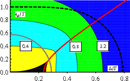
Figure 1: Contour plot of the positive imaginary part of the dimensionless root Im$[y_{1}]/\Gamma=\frac{\sqrt{3}}{2\Gamma}(S-T)$. The black area corresponds to the region where all three roots are real. The red (light gray) line corresponds to $R=0$ and the gray line to $Q=0$. The black dashed curve shows $Im[z_{1}]=-Re[z_{1}]$.

If the discriminant is positive: $Q^{3}+R^{2}>0$, $S$ and $T$ are real positive and negative, respectively. Therefore, the root $z_{0}$ is real and the two others $z_{1,2}$ are complex conjugates of each other. In the case of $Q^{3}+R^{2}<0$, $S$ and $T$ are also complex conjugate. Hence, all three roots are real negative. In this case the oscillatory behavior of the Bloch vector in Eq. (15) does not occur. This parametric area of triangular form is depicted as black in Fig.1. Its three vertices have coordinates (0,0), (1/4,0) and ($\sqrt{2/27},\sqrt{1/27}$). In the parametric area above the red line $R=0$ in Fig.1 both $R$ and $\gamma_{1}$ are negative. The $z_{0}$ non-oscillating mode of the Bloch vector in Eq. (15) decays quicker than the oscillating modes and the transient current is an infinitely oscillating function of time. Below this line $\gamma_{1}$ is positive, the amplitude of the oscillations vanishes more quickly than the first term, and the additional condition epl on the initial state of the QD should be fulfilled to observe oscillations of the transient current. Below we consider manifestations of these oscillations in the frequency dependent current response to the applied a.c. voltage of a small amplitude.

V Current response to the time dependent voltage

The change in the Bloch vector evolution by the applied a.c. voltage is described in Eq. (8) by the first and third term on its right-hand side with the evolution operator defined by Eq.(9) with $\Delta M(t^{\prime})=v\cos(\omega t^{\prime})\Lambda$. Below we will be interested in the steady regime of the evolution, when $\Gamma t\gg 1$ and the starting time of the evolution can be drawn in Eq. (8) from zero to $-\infty$. Then, contrary to the transient qubit dynamics, only the third term contributes. The evolution operator in this term can be calculated through expansion of the time-ordered exponent in Eq. (9) with respect to $\Delta M_{i}$ and we find the Bloch vector variation by the ac voltage application as a perturbative series in $v$: $\Delta\mathbf{a}(t)=\sum_{n=1}\Delta_{n}\mathbf{a}(t)$. The general term of this series $\Delta_{n}\mathbf{a}(t)$ contains multiple $m\omega$ frequency components, where $m$ is of the same parity as $n$ and runs from zero to $n$. Below we calculate explicitly the first two terms $\Delta_{1}\mathbf{a}(t)$ and $\Delta_{2}\mathbf{a}(t)$ of this series.

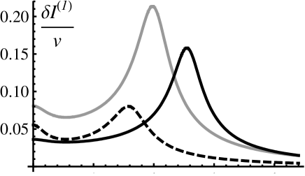
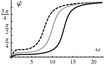
Figure 2: Normalized amplitude (upper panel) and phase shift (lower panel) of the first harmonic of the ac current $\delta I^{(1)}/v$ defined by Eqs. 20, 21 when $\Gamma=1$, $\Delta=4$. The black lines correspond to the resonant level energy $\epsilon_{d}=-10$, the gray lines to $\epsilon_{d}=-6$, and the black dashed lines to $\epsilon_{d}=-1$ .

V.1 Linear current response

In the first order of the perturbation expansion in $v$ we substitute the $S_{0}$ operator from Eq. (10) for the evolution operator in the last term on the right-hand side of Eq. (8). Choosing the contour $C$ in Eq. (10) to go from $(-0-i\infty)$ to $(-0+i\infty)$ and performing integration over $t^{\prime}$ in the last term, we further close the contour in the right half-plane and express the result through the poles contributions as

$$\frac{\Delta_{1}\mathbf{a}(t)}{v} = Re\frac{e^{i\omega t}}{i\omega-M_{0}}\Lambda\mathbf{a}(\infty)=$$

$$Re\sum\limits_{l=0}^{2}\mathbf{l}_{R}\frac{e^{i\omega t}}{i\omega-z_{l}}(\mathbf{l}_{L}|\Lambda\mathbf{a}(\infty))\ .$$

From comparison of the last part of Eq. (V.1) with Eq. (15) we conclude that in the $v$ linear response of the a.c. Bloch vector response $\Delta_{1}\mathbf{a}(t)$ coincides at times $t=\mbox{integer}\times 2\pi/\omega$ and $t=(\mbox{integer}-1/4)\times 2\pi/\omega$ with the real and imaginary parts of the spectral decomposition of the transient Bloch vector, originating from its initial state $\mathbf{a}(0)-\mathbf{a}(\infty)=\Lambda\mathbf{a}(\infty)$. The spectral decomposition of the corresponding transient current $I_{tr}(t)$ can be found from the oscillating current $\Delta_{1}I(t)=-\Gamma\Delta_{1}a_{3}(t)=\delta I^{(1)}\cos(\omega t-\varphi)$ in the following way

$$\int_{0}^{\infty}dte^{-i\omega t}[I_{tr}(t)-I_{0}]=\delta_{1}I\cdot e^{-i\varphi}\ ,$$ (20)

where $\delta I^{(1)}$ and $\varphi$ are the amplitude and the phase shift of $\Delta_{1}I(t))$. The oscillating behavior of the transient current defined by Eq. (15) emerges as a resonance in the frequency dependence of the amplitude $\delta I^{(1)}$ and as an abrupt change of the phase $\varphi$ of the first $\omega$ harmonic of the oscillating current at $\omega=\omega_{I}$ if the coefficient $\mathbf{r}_{1,3}$ at the resonant term in Eq. (V.1) is non zero.

By inversion of the matrix denominator in the first part of Eq. (V.1) we find the oscillating current as follows

$$\Delta_{1}I(t)=-2I_{0}vRe[\epsilon_{d}(i\omega+2\Gamma)e^{i\omega t}/P(i\omega)]\\$$ (21)

The amplitude of its oscillations $\delta I^{(1)}(\omega,\epsilon_{d})$ and the phase shift $\varphi(\omega,\epsilon_{d})$ are depicted in Fig. 2 for the several choices of the parameters. Here we have defined $\varphi$ so that it is positive at $\epsilon_{d}<0$ and $\omega>0$ and zero at $\omega=0$. Then it expands as $\varphi(\omega,\epsilon_{d})=-\varphi(-\omega,\epsilon_{d})$ to negative $\omega$ and through $\varphi(\omega,\epsilon_{d})=-\pi\,\mbox{sgn}(\omega)+\varphi(\omega,-\epsilon_{d})$ for $\epsilon_{d}>0$. The amplitude $\delta_{1}I(\omega,\epsilon_{d})$ is even function of both $\omega$ and $\epsilon_{d},$ namely, $\delta_{1}I(\omega,\epsilon_{d})=\delta_{1}I(\pm\omega,-\epsilon_{d}).$ The coefficient $\mathbf{r}_{1,3}$ characterizing the strength of the $\delta I^{(1)}$ resonance follows from Eq. (21) as

$$\mathbf{r}_{1,3}=-\frac{vI_{0}}{\Gamma^{2}}\frac{\epsilon_{d}(2\Gamma/3+\gamma_{1}/2+i\omega_{I})}{\omega_{I}(3\gamma_{1}-2i\omega_{I})}$$ (22)

It vanishes at the resonance $\epsilon_{d}=0$, where the deviation of the Bloch vector initial condition from its stationary value $v\Lambda\mathbf{a}(\infty)=vI_{0}/(\Gamma\Delta)[-\Gamma,\epsilon_{d},0]^{T}$ does not produce the transient current.

At small $\Gamma\ll\sqrt{\epsilon_{d}^{2}+4\Delta^{2}}$ the $\delta I^{(1)}$ resonance in Fig. 2 has Lorentzian shape centered at $\omega_{I}\approx\sqrt{\epsilon_{d}^{2}+4\Delta^{2}}$ with the width $G_{1}\approx\Gamma(1+2\Delta^{2}/\omega_{I}^{2}).$ Since the poles $z_{1,2}$ are close to the imaginary axis, if Re[$z_{1,2}]\ll\omega_{I}$, the phase shift at $\omega=\omega_{I}$ is $\varphi\approx{\small\mp}\pi/2$.

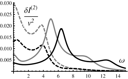
Figure 3: Normalized amplitude of the second harmonic of the ac current $\delta I^{(2)}/v^{2}$ from Eq. 24 when $\Gamma=1$, $\Delta=4$. The black line corresponds to the resonant level energy $\epsilon_{d}=10$, the gray line to $\epsilon_{d}=6$, and the black dashed line to $\epsilon_{d}=2,$ and the gray dashed line to $\epsilon_{d}=0$ .

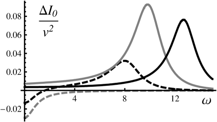
Figure 4: The frequency dependent variation of the average current $\Delta I_{0}/v^{2}$ from Eq. 26 when $\Gamma=1$, $\Delta=4$. The black line corresponds to the resonant level energy $\epsilon_{d}=10$, the gray line to $\epsilon_{d}=6$, and the black dashed line to $\epsilon_{d}=2,$ and the gray dashed line to $\epsilon_{d}=0$ .

V.2 Second-order current response

Substitution of the first $\Delta M_{I}$ order expansion of the expression for the evolution operator $S(t,t_{0})$ in Eq. (9) into the last term on the right-hand side of Eq. (8) gives us

$$\Delta_{2}\mathbf{a}(t) =$$ (23)

$$\int_{-\infty}^{t}\!\!\!\!\!\!d\tau\int_{-\infty}^{\tau}\!\!\!dt^{\prime}S_{0}(t-\tau) \Delta M(\tau)S_{0}(\tau-t^{\prime})\Delta M(t^{\prime})\mathbf{a}(\infty)\ .$$

Making use of the representation of $S_{0}$ in Eq. (10) and performing successive integration over $t^{\prime}$ and $\tau$ we find $\Delta_{2}\mathbf{a}(t)$ in Eq. (23) after closing both contours $C$ of the Laplace transformation in the right half-plane as follows

$$\Delta_{2}\mathbf{a}(t) = \frac{v^{2}}{2}Re\left\{\frac{e^{i2\omega t}}{i2\omega-M_{0}}\Lambda\frac{1}{i\omega-M_{0}}\Lambda\mathbf{a}(\infty)\right\}$$ (24)

$$-\frac{v^{2}}{2M_{0}}\Lambda Re\left\{\frac{1}{i\omega-M_{0}}\Lambda\mathbf{a}(\infty)\right\}\ .$$

The first term here describes the Bloch vector variation resulting in the second $\omega$ harmonic of the oscillating current $\Delta_{2}I(t)$, whose amplitude $\delta I^{(2)}(\omega)$ as depicted in Fig. 3 exhibits two resonances at $\omega=\omega_{I}/2$ and $\omega=\omega_{I}$ if $\Gamma$ small enough. The second term contributes to the frequency dependent deviation $\Delta I_{0}$ due the a.c. voltage of the average steady current from the stationary current $I_{0}$. From comparison of this term with the right side of Eq. (V.1) we express this current shift through the first order variation of the Bloch vector:

$$\Delta I_{0}=-\frac{vI_{0}}{2\Gamma\Delta}(\mathbf{x}|\Delta_{1}\mathbf{a}(0)),$$ (25)

where $\mathbf{x}=[\Gamma,\epsilon_{d},0]^{T}$. Therefore, it combines the spectral decompositions of the transient dynamics of the first two components of the Bloch vector. We use its explicit form:

$$\Delta I_{0}=-\frac{v^{2}I_{0}^{2}}{2\Gamma\Delta^{2}}Re\left[\frac{P_{1}(i\omega)}{P(i\omega)}\right],$$ (26)

where

$$P_{1}(z) = \left(\Gamma^{2}-\epsilon_{d}^{2}\right)x^{2}+\left(\Gamma^{3}-3\Gamma\epsilon_{d}^{2}\right)x+2\Gamma^{2}\left(2\Delta^{2}-\epsilon_{d}^{2}\right)$$

$$\ \ \ x = z+\Gamma$$ (27)

to demonstrate in Fig. 4 that at finite $\epsilon_{d}\neq 0$ it exhibits a single resonance at $\omega=\omega_{I}$ with the width $G_{1}\approx\Gamma(1+2\Delta^{2}/\omega_{I}^{2})$. It transforms into the negative Lorentz function $\Delta I_{0}/v^{2}=-I_{0}^{2}\Gamma/(\omega^{2}+\Gamma^{2})/(2\Delta^{2})$ at the resonant level position as a consequence of the pure exponential decay dynamics of the first Bloch vector component.

VI Conclusion

The tunneling of spinless electrons through an interacting resonant level of a QD into an empty collector has been studied in the especially simple, but realistic system, in which all sudden variations in charge of the QD are effectively screened by a single tunneling channel of the emitter. As a result the time evolution of the system in question has been reduced to the dynamics of a dissipative two-level model. Its off-diagonal coupling parameter $\Delta$ is equal to the bare emitter tunneling rate $\Gamma_{e}$ renormalized by the large factor $\sqrt{D/(\pi\Gamma_{e})},$ whereas the dumping parameter $\Gamma$ coincides with the tunneling rate of the collector. For a constant bias voltage the short time transient behavior of this model was studied in epl and it has been shown that the FES in the tunneling current dependence on the voltage should be accompanied by oscillations of the time-dependent transient tunneling current in the wide range of the model parameters. In particular, they occur if the emitter tunneling coupling $\Delta$ or the absolute value of the resonant level energy $|\epsilon_{d}|$ are large enough in comparison with the collector tunneling rate $\Gamma$ and either $\Delta>\Gamma/4$ or $\epsilon_{d}^{2}>\Gamma^{2}/27$ holds.

Although these oscillations should confirm the emergence of the qubit composed of an electron-hole pair at the QD and its coherent dynamics in agreement with the FES theory it could be difficult to observe them directly, since this involves measurement of the time dependent transient current averaged over its quantum fluctuations. Therefore, in this work we have studied manifestations of the coherent qubit dynamics in the collector a.c. response to a periodic time dependent voltage of the frequency $\omega$.

We have calculated the steady long time dependence of the qubit Bloch vector and the tunneling current perturbatively in any order in the a.c. voltage amplitude and further have used this expansion to describe the frequency dependence of the parameters of the steady a.c. response. In particular, we have found that the oscillatory behavior of the transient current results in the non-zero frequency resonances in the amplitudes dependence of the a.c. harmonics and in the jumps of the a.c. harmonics phase shifts across the resonances. In the first order of this expansion only the first $\omega$ harmonic arises in the a.c. response. Its amplitude exhibits resonant behavior at $\omega=\omega_{I}$ for a wide range of the model parameters, where $\omega_{I}$ is the frequency of the oscillating transient current. In this order the a.c. response is directly related to the spectral decomposition of the transient current produced by the specific initial disturbance of the qubit stationary state by the applied voltage. In the higher orders of the a.c. expansion also the higher harmonics emerge and the corresponding resonances occur at the fractions of $\omega_{I}$. The found results confirm that the observation of the a.c. tunneling into the collector opens a realistic way for the experimental demonstration of the coherent qubit dynamics and should be useful for further identification of the FES in tunneling experiments.

We have performed our calculations in dimensionless units with $\hbar=1$ and $e=1,$ therefore, the unit of the a.c. admittance in Fig. 2 is $e^{2}/\hbar\approx 2.43\cdot 10^{-4}$S. In the experiments lar ; lar1 the collector tunneling rate is $\Gamma\approx 0.1\,meV$ and the coupling parameter $\Delta\approx 0.016\,meV$. This corresponds to the stationary current equal to $I_{0}\approx 1.2\,nA$ at $\epsilon_{d}=0$. To observe the regime of the induced oscillations shown in Fig. 2 one can increase the collector barrier width to obtain the heterostructure with $\Delta=4\Gamma$. Then, with $\Delta=0.016\,meV$ and $\Gamma\approx 4\mu eV$, the stationary current at the resonant level position is $I_{0}=0.94\,nA$. The unit of frequency $\omega$ in Figs. 2-4 for this value of $\Gamma$ is $6.08\cdot 10^{9}s^{-1}$. With the amplitude of the oscillating voltage equal to $v=1\mu V$ we find that the peak of the a.c. amplitude of its first harmonic is $\delta I_{mx}^{(1)}=53\,pA$. It occurs at $\nu_{I}=\omega_{I}/(2\pi)=9.6\,GHz$ for $\epsilon_{d}=-0.024\,meV$ (gray curves in Fig. 2). At the same parameters $v$ and $\epsilon_{d}$ the resonance of the a.c. second harmonic (gray curve in Fig. 3) takes place at $\nu_{I}/2=4.8\,GHz$ and its amplitude is $\delta I_{mx}^{(2)}=1.4\,pA$.

VII Acknowledgment

The work was supported by the Foundation for Science and Technology of Portugal and by the European Union Seventh Framework Programme (FP7/2007-2013) under grant agreement n^o PCOFUND-GA-2009- 246542 and Research Fellowship SFRH/BI/52154/2013. It was also funded (V.P.) by a Leverhulme Trust Research Project Grant RPG-2016-044.

References

- (1) G. D. Mahan, Phys. Rev. 163, 612 (1967).
- (2) P. Nozieres and C. T. de Dominicis, Phys. Rev. 178, 1097 (1969).
- (3) K. Ohtaka and Y. Tanabe, Phys. Rev. B 30, 4235 (1984).
- (4) B. Muzykantskii, N. d Ambrumenil, and B. Braunecker, Phys. Rev. Lett. 91, 266602, (2003).
- (5) D. A. Abanin, L. S. Levitov, Phys. Rev. Lett. 94,186803, (2005).
- (6) P. H. Citrin, Phys. Rev. B 8, 5545 (1973).
- (7) P. H. Citrin, G. K. Wertheim, and Y. Baer, Phys. Rev. B 16, 4256 (1977).
- (8) K. A. Matveev and A. I. Larkin, Phys. Rev. B 46, 15337 (1992).
- (9) A. K. Geim, P. C. Main, N. La Scala Jr., L. Eaves, T. J. Foster, P. H. Beton, J. W. Sakai, F. W. Sheard, M. Henini., G. Hill and M. A. Pate, Phys. Rev. Lett. 72, 2061 (1994)
- (10) I. Hapke-Wurst, U. Zeitler, H. Frahm, A. G. M. Jansen, R. J. Haug, and K. Pierz, Phys. Rev. B 62, 12621 (2000).
- (11) H. Frahm, C. von Zobeltitz, N. Maire, and R. J. Haug, Phys. Rev. B 74, 035329 (2006).
- (12) M. Ruth, T. Slobodskyy, C. Gould, G. Schmidt, and L. W. Molenkamp, Applied Physics Letters 93, 182104 (2008).
- (13) A. J. Leggett et al., Rev. Mod. Phys. 59, 1 (1987).
- (14) O. Katsuba and H. Schoeller, Phys. Rev. B 87, 201402(R) (2013).
- (15) N. Maire, F. Hohls, T. Lüdtke, K. Pierz, and R. J. Haug, Phys. Rev. B 75, 233304 (2007).
- (16) N. Ubbelohde et al., Sci. Rep. 2, 374 (2012).
- (17) K. Roszak and T. Novotný, Phys. Scr. T151 014053 (2012).
- (18) V.V. Ponomarenko and I. A. Larkin, EPL 113, 67004 (2016).
- (19) K. Schotte and U. Schotte, Phys. Rev. 182, 479 (1969).
- (20) H.T. Imam, V.V. Ponomarenko, and D.V. Averin, Phys. Rev. 50, 18288 (1994).
- (21) I.A. Larkin, E.E. Vdovin, Yu.N. Khanin, S. Ujevic and M. Henini, Phys. Scripta, 82, 038106, (2010).
- (22) N. Jacobson, Basic algebra 1 (2nd ed.), Dover, (2009), ISBN 978-0-486-47189-1
- (23) I.A. Larkin, Yu.N. Khanin, E.E. Vdovin, S. Ujevic and M. Henini, J. Phys.: Conf. Ser. 456, 012024, ( 2013).