Exact solutions and phenomenological constraints from massive scalars in a Gravity’s Rainbow spacetime

Abstract

We obtain the exact (confluent Heun) solutions to the massive scalar field in a Gravity’s Rainbow Schwarzschild metric. With these solutions at hand, we study the Hawking radiation resulting from the tunneling rate through the event horizon. We show that the emission spectrum obeys non-extensive statistics and is halted when a certain mass remnant is reached. Next, we infer constraints on the rainbow parameters from recent LHC particle physics experiments and Hubble STIS astrophysics measurements. Finally, we study the low frequency limit in order to find the modified energy spectrum around the source.

Key words: Rainbow gravity, Hawking radiation, microscopic black holes, fine structure constant.

I Introduction

The meaning of the theory of General Relativity (GR) has been brilliantly resumed by J. A. Wheeler in a simple and celebrated sentence: “Matter tells spacetime how to curve, and spacetime tells matter how to move”. This aphorism emphasizes the fulcrum of the Einstein’s theory, according to which the gravitational field reveals itself as a curvature of spacetime Wheeler . This picture works very well for a massive body curving the spacetime where a (not very high-energy) particle is moving in. However, at ultra high-energies the theory needs serious revision for the concept of spacetime coordinates itself has to be reconsidered.

Indeed, the formal necessity of a tiny-scale (so-called UV) modification of GR arises from the non-renormalizability of a quantum field theory of gravity. This can be seen from the high-energy divergent diagrams in Feynman loop-expansion stelle . A way to deal with this issue is to insert higher-order derivative terms in the Lagrangian which modify the UV graviton propagator stelle . But the problem is that higher-order time derivatives in the equations of motion lead to ghosts. In order to keep the good and remove the bad, P. Horava introduced a asymmetric Lifshitz scaling between space and time Horava such that higher order spatial-derivatives are not accompanied by higher order time- ones in the UV regime. This particular Lorentz symmetry violation allows power-counting renormalizability while avoids ghosts and GR arises as an infrared fixed point.

An alternative approach is to modify the metric instead of reshaping the action. This so-called Rainbow Gravity scenario MS2004 radically changes the GR framework since, according to it, the UV deformed metric introduces the asymmetry between space and time but now it is done through the energy of the probe. This correction has been shown to fix one loop divergences, avoiding the need of a renormalization scheme garattini . This is a great advantage which makes the rainbow proposal a source of constant investigation, e.g.2017 (a connection with the Horava-Lifshitz gravity can be found in garattini2 ).

Rainbow gravity can be obtained as a generalization to curved spacetimes of the so-called Doubly Special Relativity (DSR) MSmolin1 ; MSmolin2 ; Camelia . In DSR the transformation laws in energy-momentum space are nonlinear. The dual space, $(x,t)$, is thus endowed with a nontrivial quadratic invariant, namely, an energy-dependent metric tensor. It means that if a given observer measures a particle (or wave) with energy $E$, then he concludes that this probe feels a metric $\mathrm{g}_{ab}(E)$. But, on the other hand, a different observer will measure instead $E^{\prime}\neq E$, and will therefore assign to the particle’s motion different metric tensor elements $\mathrm{g}_{ab}(E^{\prime})$. This argument, valid in flat spacetime, carries over locally to curved spacetimes using the equivalence principle. As a consequence, the invariant norm is no longer bilinear and leads to modified dispersion relations.

In DSR the laws of energy-momentum conservation still hold in all inertial frames but then again they are non-linear. One important reason for the DSR proposal is that the energy scale which establishes the boundary between the quantum and classical characterization of spacetime, $E_{P}$, can be assumed as an invariant in the sense that all inertial observers agree on whether a particle has more, or less, than this energy. Interestingly, this works out an otherwise inconvenience; namely, that the threshold between the quantum and the classical description can depend on the speed of the observer MS2004 .

The first accomplishment in DSR Amati implies a deformed Lorentz symmetry such that the standard energy-momentum relations in flat spacetime are modified by Planck scale corrections of the form

$$E^{2}\,f^{2}(\omega/\omega_{P})-(pc)^{2}\,g^{2}(\omega/\omega_{P})=m^{2}c^{4},$$ (1)

where $m$ is the rest frame mass of the particle with energy-frequency $\omega$ as seen by an inertial observer, and $\omega_{P}$ is the Planck energy-frequency $E_{P}=\hbar\omega_{P}$. Global Lorentz invariance is in fact an accidental symmetry related to a particular solution of General Relativity. Thus, whether it is broken or modified it is only a symmetry emerging at low energies from a quantum theory of gravity and is just approximate.

It is generally accepted that at sufficiently high energies the geometry of spacetime should be described by a quantum theory in which General Relativity is replaced by a quantum mechanical description of the spacetime coordinates. It is also believed that the Planck energy $E_{P}=\sqrt{\hbar c^{5}/G}$ establishes the threshold that separates the classical description from the quantum description of gravity. Above the Planck scale a continuous spacetime manifold loses consistency for quantum effects become uncontrollable and a metric approach becomes impracticable. Thus, rainbow gravity is concerned with the effects on the propagation of particles with energies below $E_{P}$ but whose wavelengths are much shorter than the local radius of curvature of spacetime. Of course, to be consistent with the standard theory, the functions $f(\omega/\omega_{P})$ and $g(\omega/\omega_{P})$ which appear in Eq. (1) must tend to unity near $E_{P}$. In this context, a generalized uncertainty principle (GUP) is often introduced in order to account for this fuzzy microscopic structure of spacetime and to avoid the singularities of the general relativity Maggiore1 ; Maggiore2 .

In this work we will adopt a semiclassical approach inspired in loop quantum gravity Smolin0 to study an uncharged scalar field placed in a spherically symmetric spacetime characterized by the aforementioned MDR functions defined as

$$f(\omega/\omega_{P})=1,\ \ \ \ \ \ g(\omega/\omega_{P})=\sqrt{1-\xi(\omega/\omega_{P})^{s}},$$ (2)

where $\xi>0$, and $s$ is a positive integer of order one. We will obtain the exact wave solutions to the scalar field and later on analyze them near the event horizon in order to compute the Hawking radiation via quantum tunneling through this frontier. Constraints on these rainbow parameters will be obtained by considering particle physics experiments related to negative results regarding the creation of microscopic black holes in the LHC as well as galactic measurements of the fine-structure constant made by the Hubble Space Telescope (STIS) from a white dwarf spectrum.

The paper is organized as follows: In section II we obtain the exact solutions of a massive scalar field in the rainbow Schwarzschild metric, then study the Hawking radiation, and thereafter calculate the energy eigenspectrum and infer new constraints on the rainbow parameters. Finally, in section III, we draw the conclusions.

II Massive Scalar Field in Rainbow Schwarzschild Spacetime

Although it has been a long-studied subject, the massive scalar field in a Schwarzschild spacetime (see Frolov and references therein) lacked of an exact solution until recently Fiziev3 . Now, it is known that its whole space spectrum is formally given in terms of Heun’s functions Ronveaux combined with elementary functions. Here we will employ an analytic approach in order to solve such a problem, this time considering a gravity’s rainbow metric.

II.1 Solutions

Our task is solving the rainbow gravity covariant Klein-Gordon equation of massive scalars minimally coupled to the Schwarzschild gravitational field

$$\left[\frac{1}{\sqrt{-\mathrm{g}}}\partial_{\mu}\left(\mathrm{g}^{\mu\nu}\sqrt{-\mathrm{g}}\partial_{\nu}\right)+m^{2}\right]\Psi=0\ ,$$ (3)

(where natural units $c\equiv\hbar\equiv 1$ are used).

The gravitational background generated by a static uncharged compact object is given by the Schwarzschild metric now depending on the rainbow functions $f(\omega/\omega_{P})$ and $g(\omega/\omega_{P})$. In spherical coordinates the square line-element invariant reads JMathPhys.8.265

$$ds^{2}=f^{-2}(\omega/\omega_{P})h(r)dt^{2}-g^{-2}(\omega/\omega_{P})[h(r)^{-1}dr^{2}-r^{2}d\Omega^{2}],$$ (4)

where $h(r)=\left(1-\frac{r_{s}}{r}\right)$, $r_{s}=2MG$ is the Schwarzschild radius, $d\Omega^{2}=d\theta^{2}+\sin^{2}\theta\ d\phi^{2}$, $G=G(0)$ is the Newton’s universal gravitational constant and $M$ is the mass of the source. By symmetry arguments we assume that solutions of Eq. (3) can be factored as follows

$$\Psi(\mathbf{r},t)=R(r)Y_{l}^{m_{l}}(\theta,\phi)\mbox{e}^{-i\omega t},$$ (5)

where $Y_{l}^{m_{l}}(\theta,\phi)$ are the spherical harmonic functions. Inserting Eq. (5) and the metric given by Eq. (4) into (3), we obtain the following radial equation

$$\frac{d}{dr}\left[r(r-2GM)\frac{dR}{dr}\right]+\left(\frac{r^{3}\tilde{\omega}^{2}}{r-2GM}-\tilde{m}^{2}r^{2}-\lambda_{lm_{l}}\right)R=0,$$ (6)

where $\lambda_{lm_{l}}=l(l+1)$ and

$$\tilde{\omega} = \frac{\omega}{g(\omega/\omega_{P})},$$ (7)

$$\tilde{m} = \frac{m}{g(\omega/\omega_{P})}.$$

The expression given by Eq. (6) has singularities at $r=(a_{1},a_{2})=(0,2GM)$ and $\infty$, and can be transformed into a Heun equation by using

$$x=\frac{r-a_{1}}{a_{2}-a_{1}}=\frac{r-2GM}{2GM}\ .$$ (8)

Let us introduce the function $Z(x)$ such that

$$R(x)=Z(x)[x(x-1)]^{-1/2},$$ (9)

and set henceforth $G=1$. Then, differential Eq. (6) transforms into

$$\frac{d^{2}Z}{dx^{2}}+\left[A_{1}+\frac{A_{2}}{x}+\frac{A_{3}}{x-1}+\frac{A_{4}}{x^{2}}+\frac{A_{5}}{(x-1)^{2}}\right]Z=0,$$ (10)

where the coeficients $A_{1}$, $A_{2}$, $A_{3}$, $A_{4}$, and $A_{5}$ are given by

$$A_{1}=-4M^{2}\left(\tilde{m}^{2}-\tilde{\omega}^{2}\right)\ ;$$ (11)

$$A_{2}=\frac{1}{2}+\lambda_{lm_{l}}+4M^{2}\left(\tilde{m}^{2}-2\tilde{\omega}^{2}\right)\ ;$$ (12)

$$A_{3}=-\frac{1}{2}-\lambda_{lm_{l}}\ ;$$ (13)

$$A_{4}=\frac{1}{4}+4M^{2}\tilde{\omega}^{2}\ ;$$ (14)

$$A_{5}=\frac{1}{4}\ .$$ (15)

The general solution to Eq. (10) over the entire range $0<x\leq\infty$ is given by Horacio2

$$R(x) = C_{1}\mbox{e}^{\frac{1}{2}\alpha x}x^{\frac{1}{2}\beta}\mbox{HeunC}(\alpha,\beta,\gamma,\delta,\eta;x)$$ (16)

$$+ C_{2}\mbox{e}^{\frac{1}{2}\alpha x}\ x^{-\frac{1}{2}\beta}\mbox{HeunC}(\alpha,-\beta,\gamma,\delta,\eta;x)\ ,$$

where $C_{1}$ and $C_{2}$ are constants, and the parameters $\alpha$, $\beta$, $\gamma$, $\delta$, and $\eta$ explicitly written in terms of the rainbow’s function are given by:

$$\alpha=-4M\sqrt{\frac{m^{2}-\omega^{2}}{1-\xi(\omega/\omega_{P})^{s}}};$$ (17a)

$$\beta=\frac{i4M\omega}{\sqrt{1-\xi(\omega/\omega_{P})^{s}}}\ ;$$ (17b)

$$\gamma=0\ ;$$ (17c)

$$\delta=\frac{4M^{2}\left(m^{2}-2\omega^{2}\right)}{1-\xi(\omega/\omega_{P})^{s}};$$ (17d)

$$\eta=-l(l+1)-\frac{4M^{2}\left(m^{2}-2\omega^{2}\right)}{1-\xi(\omega/\omega_{P})^{s}}.$$ (17e)

This is the sum of two linearly independent solutions of the confluent Heun differential equation provided $\beta$ is not an integer Ronveaux .

It is also worth mentioning some pioneering work done in this direction japan3 , where analytic solutions to the (massless) Regge-Wheeler and Teukolsky equations are found as a series of hypergeometric and Coulomb wavefunctions with different regions of convergence. This has been used in binidamour to compute the post-Minkowskian expansion of Regge-Wheeler-Zerilli black hole perturbation theory to calculate a fourth order post-Newtonian approximation of the main radial potential describing the gravitational interaction of two bodies. For a massive scalar particle, the effects of the self-force upon the orbits of a Schwarzschild black hole have been computed in detweiler .

II.2 Uncompleted Hawking Radiation

The exterior outgoing wave solutions at the event horizon of a Schwarzschild black hole are obtained by taking $x\rightarrow 0^{+}$ in Eq. (16) for positive frequencies. If we also consider the temporal part of the wave function, the result is

$$\Psi_{out}(r\simeq 2M^{+})\simeq C_{1}e^{-i\omega t}(r-2M)^{2iM\tilde{\omega}}.$$ (18)

Let us now examine the variable

$$r_{*}=g^{-1}\,(\omega/\omega_{P})\left[r+2M\log{\left|\frac{r-2M}{2M}\right|}\right]$$ (19)

inspired in the conventional $(\xi=0)$ tortoise coordinate (which approaches $-\infty$ when $r\rightarrow r_{s}$), appropriate to analyze perturbations in the spherically symmetric gravitational field Frolov . Considering Eddington-Finkelstein coordinates, we define $v=t+r_{*}$ yielding

$$\Psi_{out}(r\simeq 2M^{+})=C_{1}e^{-i(\omega v-\tilde{\omega}r)}(2M)^{-2iM\tilde{\omega}}(r-2M)^{4iM\tilde{\omega}}.$$ (20)

Following Damour we now consider the analytic extension of the solution to the interior region ($r\simeq 2M^{-}$) by means of a rotation in the complex plane $(r-2M)\rightarrow(2M-r)e^{-i\pi}$ in Eq.(20). Thus, one has

$$\Psi_{out}(r\simeq 2M^{-})=C_{1}e^{-i(\omega v-\tilde{\omega}r)}(2M)^{-2iM\tilde{\omega}}(2M-r)^{4iM\tilde{\omega}}e^{4\pi M\tilde{\omega}}.$$ (21)

With these two expressions we can calculate the transmission coefficient through the horizon, namely the tunneling rate, defined as

$$\Gamma_{ev}=\left|\frac{\Psi_{out}(r\simeq 2M^{+})}{\Psi_{out}(r\simeq 2M^{-})}\right|^{2}=\exp{\left[-\frac{8\pi M\omega}{g(\omega/\omega_{P})}\right]}.$$ (22)

It is worth noting that rainbow gravity black holes never evaporate completely. Unlike the ordinary Schwarzschild black hole, the rainbow one halts outwards tunneling when it reaches a certain nonzero minimal value which equals the critical mass (i.e. the mass which avoids the BH temperature turning imaginary) remnant . This remnant mass can be calculated by making $\Gamma_{ev}=0$ in Eq. 22 assuming a generalized position-momentum uncertainty principle.

This GUP can be motivated on general grounds by the intuition that the solution of the quantum gravity problem would need an absolute planckian limit of the size of the collision region Amelino_IJMP ; Amelino_CQG . So far, it is consensual both in String Theory and Loop Quantum Gravity that a GUP compatible with a (leading order correction) logarithmic-area growth of BH entropy should be of the the form

$$\delta x\geq\frac{1}{\delta p}+\lambda L_{P}^{2}\delta p+O(L_{P}^{3}\delta p^{2})$$ (23)

where the coefficient $\lambda$ should take a value of roughly the ratio between the square of the string length and the square of the Planck length $L_{P}$. While in nonrelativistic quantum mechanics a particle of any energy can always be sharply localized (at the price of losing any information on the conjugate momentum), within quantum field theory it can only happen in the infinite-energy limit. However, at the quantum gravity level the intuition is that such a sharp localization should disappear and uncertainty could be recoded in a relation of the type

$$E\geq\frac{1}{\delta x}[1-\Delta(L_{P},\delta x)]$$ (24)

where $\Delta(L_{P},\delta x)$ should be such that $E\rightarrow\infty$ at some nonzero $\delta x$. According to the usual argument of quantum mechanics, when the position of a particle of mass $M$ (at rest) is being measured by a procedure involving a collision with a photon of momentum $p_{\gamma}$, we have $\delta p_{\gamma}\geq 1/\delta x$ where $\delta p_{\gamma}$ is the photon momentum uncertainty and $\delta x$ is the position uncertainty of the $M$ particle. Using the special relativity Heisenberg’s uncertainty principle, it also means that $\delta E_{\gamma}\geq 1/\delta x$ which yields naturally $M\geq 1/\delta x$ since we need $\delta E_{\gamma}\leq M$ in order not to disturb completely the system being measured. Applying a boost the relation results in $E\geq 1/\delta x$, which on a rainbow gravity basis carries into $E\geq[1+\sum a_{k}(L_{P}/\delta x)^{k}]/\delta x$, as stated in Eq. (24).

In our context, assuming that the test particle is a massless scalar localized within the BH event horizon $r_{s}=2M$, its frequency uncertainty results $\delta\omega\geq(2M)^{-1}$ which at leading order implies then again $\omega\geq(2M)^{-1}$ Ali . The remnant mass of the BH, $M_{r}$, can be therefore obtained by making $g(\omega/\omega_{P})=0$ in Eq. (22), i.e. considering null evaporation rate for the minimal $\omega$ value. After some straightforward calculation, we obtain the following expression for $M=M_{r}$ as a function of the rainbow parameters

$$M_{r}=\frac{\xi^{1/s}}{2}M_{P},$$ (25)

where $M_{P}$ is the Planck mass.

Should we know the phenomenological mass value of the remnant, we could calculate a lower bound to the rainbow parameters. From recent negative results regarding microscopic black holes in the CMS experiment at CERN’s Large Hadron Collider we can so far exclude BH masses below 6.2 TeV Sirunyan . This allows establishing a constraint in the parameters given by

$$6.2\mathrm{TeV}<\frac{\xi^{1/s}}{2}2\times 10^{16}\mathrm{TeV}\Rightarrow\xi^{1/s}>6.2\times 10^{-16},$$ (26)

which for a conservative (simple) assumption of $s=1$ and $s=2$, result in $\xi>6.2\times 10^{-16}$ and $\xi>3.8\times 10^{-31}$, respectively. Other constraints on this parameter calculated from data obtained in the ATLAS experiment were pointed out in Ali2 , including those related to extra-dimensional considerations.

Let us now focus on the grey-body spectrum emitted from the rainbow black hole. Its distribution function, or occupation number $n_{\omega}$, is given by Horacio3

$$n_{\omega}=\frac{\Gamma_{ev}}{1-\Gamma_{ev}}=\frac{1}{e^{{}^{q}(\omega)8\pi M\omega}-1},$$ (27)

where $q(\omega)=g^{-1}(\omega/\omega_{P})$ happens to be the Tsallis parameter associated with an incomplete non-extensive entropy (see Wang and references therein) and ${8\pi M}$ is the inverse of the usual Hawking temperature associated with a blackbody (Planck) spectrum, ${T}^{-1}_{H}$.

Nonextensivity has already been found in astrophysical contexts associated with the dynamics of systems under long range interactions at long and short distances tsallis ; japan ; chaos ; cbpf ; PLB2016 . The nonextensive statistical parameters have been shown to have important physical meaning in dictating the final mass of the formed black hole through the scaling laws found in the asymptotic regimes of strong and weak rates of mass loss, respectively cbpf .

At ultra high energies, there is an alternative to the GUP above discussed. Since gravitational back reaction dodge testing spacetime, its description as a smooth manifold appears as a practical mathematical hypothesis. It comes then natural to soften this assumption and conceive a more general noncommutative discretized spacetime endowed with uncertainty relations among the spacetime coordinates themselves. Thus, noncommutative geometry gets into matter also. A possible connection between results in these two scenarios is found in chaos by means of a relation between the parameters of the corresponding theories through nonextensive thermodynamics outcomes.

Note that differently from previous work on the subject, the expression found above, Eq. (27), shows a significant deviation from the usual spectrum, particularly because the parameter now depends on the particle’s energy. Indeed, from Eq. (27) we can see that the Hawking temperature in rainbow gravity can be defined by

$$\tilde{T}_{H}=\frac{1}{8\pi M\,\,q(\omega)}=\frac{1}{8\pi M}\sqrt{1-\xi\left(\frac{\omega}{\omega_{P}}\right)^{s}},$$ (28)

which as expected returns the standard ${T}_{H}$ value for $\xi=0$. In Fig.1 below we show (a magnification of) the dependence of the emitted energy density per frequency unit, $\rho(\omega)=\omega^{3}n_{\omega}$ for some values of $\xi$. Notice that the resulting UV energy density (above 0.2) gets lower as the rainbow parameter grows. It might be interpreted as a shift resulting from the fact that the particle’s energy is being partially spent in deforming the spacetime otherwise unaffected, as in ordinary GR. On the other hand, the spectral emissivity grows in the middle region, near the maximum. As expected, the curves are practically indistinguishable at low non-planckian energies.

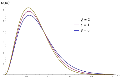
Figure 1: Energy density $\rho(\omega)=\omega^{3}n_{\omega}$ emitted by a rainbow black hole for growing values of the rainbow parameter, $\xi$, as a function of the frequency. We set $s=2$ and $T=0.1$ in Planck units.

II.3 Variable Fine Structure Constant

Now, our aim is setting an upper bound on $\xi$ from current astrophysical measurements. Making explicit the linear dependence of $\tilde{T}_{H}$ with $\hbar$ in eq.(28), we can ascribe all the rainbow dependence to a modified Planck constant, and define

$$\tilde{\hbar}=\hbar g(\omega/\omega_{P})=\hbar\sqrt{1-\xi\left(\frac{\omega}{\omega_{P}}\right)^{s}}.$$ (29)

Now, since the fine structure constant ${\alpha}$ is inversely proportional to $\hbar$ we can define a modified fine structure $\tilde{\alpha}$

$$\tilde{\alpha}=\frac{\alpha}{\sqrt{1-\xi\left(\frac{\omega}{\omega_{P}}\right)^{s}}}\approx\alpha\left[1+\frac{\xi}{2}\left(\frac{\omega}{\omega_{P}}\right)^{s}\right]$$ (30)

to take place in strong gravitational scenarios.

Hence, considering the most recent data on the relative fine structure constant in the gravitational field of a white dwarf, one verifies that $\Delta\alpha/\alpha\approx 10^{-5}$ Barrow as registered by the Hubble Space Telescope STIS from the absorbtion spectra of metal lines of G191-B2B. From this we can get a constraint on $\xi$ given by

$$10^{-5}\gtrsim\frac{\xi}{2}\left(\frac{\omega}{\omega_{P}}\right)^{s}\Rightarrow\xi\lesssim 2\times 10^{-5}\left(\frac{\omega_{P}}{\omega}\right)^{s}.$$ (31)

For a surface temperature of 60,000$-$70,000 K Rauch , this yields $\xi\lesssim 4\times 10^{22}$ for $s=1$. This upper bound gets of course higher for higher values of $s$ (see Steinhardt for a discussion of some theoretical models). A comprehensive investigation in Ref. MNRAS2012 suggests that a spatial variation of $|\Delta\alpha/\alpha|$ is in general compatible with $10^{-5}$ which puts the same upper bound on $\xi$. Finally, in the domain of atomic physics the authors of rubidio obtain a bound to the uncertainty in the gravitational gradient in an experiment involving the recoil velocity of ${}^{87}Rb$ atoms in a vertical lattice. In this case it yields $\xi\lesssim 2.8\times 10^{23}$ for $s=1$. Constraints on $s$ are also exhibited in Table I below, for these scenarios.

II.4 Gravitational Quantum Energy Levels

In this subsection, we will determine the energy eigenvalues of the massive scalar in a strong gravitational field by setting boundary conditions at the asymptotic region. In order to annul the general solution at infinity we impose a necessary condition in Eq. (16) which guarantees $R(x)$ to be a finite polynomial.

We start considering the confluent solution in the disk $|z|<1$ defined by the series expansion

$$\text{HeunC}(\alpha,\beta,\gamma,\delta,\eta,z)=\sum_{n=0}^{\infty}v_{n}(\alpha,\beta,\gamma,\delta,\eta)z^{n},$$ (32)

together with the condition $\text{HeunC}(\alpha,\beta,\gamma,\delta,\eta,0)=1$. The coefficients $v_{n}(\alpha,\beta,\gamma,\delta,\eta)$ are determined by a three-term recurrence relation

$$A_{n}v_{n}=B_{n}v_{n-1}+C_{n}v_{n-2}$$ (33)

with initial conditions $v_{-1}=0,\,\,v_{0}=1$ Fiziev . Here

$$\hskip 0.0ptA_{n} = 1+{\frac{\beta}{n}}$$ (34)

$$\hskip 0.0ptB_{n} = 1+{\frac{-\alpha+\beta+\gamma-1}{n}}+{\frac{\eta-(-\alpha+\beta+\gamma)/2-\alpha\beta/2+\beta\gamma/2}{n^{2}}}$$ (35)

$$\hskip 0.0ptC_{n} = {\frac{\alpha}{n^{2}}}\left({\frac{\delta}{\alpha}}+{\frac{\beta+\gamma}{2}}+n-1\right).$$ (36)

Thus, in order to have a polynomial confluent Heun function (16), we must impose the so called $\delta_{N}$ and $\Delta_{N+1}$ conditions

$$\frac{\delta}{\alpha}+\frac{\beta+\gamma}{2}+1 = -N$$ (37)

$$\Delta_{N+1} = 0$$ (38)

where $N$ is a non-negative integer Ronveaux . For further details see also Fiziev . From Eq. 37, we obtain the following expression for the energy levels

$$n+g^{-1}(\omega/\omega_{P})\left[2iM\omega-\frac{M\left(2\omega^{2}-m^{2}\right)}{\sqrt{m^{2}-\omega^{2}}}\right]=0,$$ (39)

where $n=N+1$.

Let us now consider the low energy regime $\omega M\ll 1$, in which the particle probe is not absorbed by the black hole. According to Eq. (22), in the limit there will be no tunneling into the event horizon of the rainbow black hole since

$$\lim_{\omega M\rightarrow 0}e^{-8\pi M\tilde{\omega}}=1$$ (40)

and therefore $\Gamma_{abs}=1-\Gamma_{ev}\rightarrow 0.$

Stationary bound-state solutions are formed by waves that propagate in opposite directions, with $\omega\in\Re$. In the present case, these are sums of outward matter waves coming from the event horizon superposed with inward matter waves moving towards the horizon, thereafter tunneling in through the Regge-Wheeler barrier Fiziev4 . Interestingly, the condition of no waves coming out from (nor going into) the horizon introduces complex valued frequencies which correspond to quasi-bound states BhabaniGrain .

Rewriting Eq. 39 for $\omega M\ll 1$, we obtain

$$\xi\omega^{s+2}-\xi m^{2}\omega^{s}-\omega^{2}+2m\omega^{(0)}_{n}+m^{2}=0,$$ (41)

where $\omega_{n}^{(0)}=-m^{3}M^{2}/2n^{2}$, with $n=1,2,3...$, are the gravitational Bohr levels (recall that in the present units, $\omega_{P}=1$).

Interestingly, for $s=1$ equation (41) has two complex omega solutions and a real one but it diverges as $\xi$ approaches zero which we also disregard. For $s=2$ there is only one relevant solution and it is given by

$$\omega_{n}=\sqrt{\frac{m^{2}}{2}+\frac{1}{2\xi}-\frac{\sqrt{m^{4}\xi^{2}-2m^{2}\xi-8m\xi\omega_{n}^{(0)}+1}}{2\xi}}.$$ (42)

For $\xi\rightarrow 0$ the corresponding bound state energies coincide with the energy spectrum given in Barranco ; CelioEPL . At first order in $\xi$, the gravitational Bohr levels are given by

$$\omega_{n}^{2}\approx m^{2}+2m\omega_{n}^{(0)}+\;\xi(2m^{3}\omega_{n}^{(0)}+4m^{2}\omega_{n}^{(0)^{2}})+\dots.$$ (43)

III Closing remarks

In this paper, we have presented the analytic solution to the Klein-Gordon equation of a massive scalar in the gravity’s rainbow Schwarzschild spacetime. Analyzing both the exterior and interior outgoing wavefunctions at the event horizon of a black hole we calculated the tunneling rate of test particles through this boundary. We have demonstrated that black hole evaporation is incomplete and stops at a remnant mass compatible with a generalized uncertainty principle. Next, we have evinced that the scalar emission spectrum (emitted particle occupation number) is associated with an incomplete non-extensive statistics where the Tsallis parameter is the rainbow function $g^{-1}(E/E_{P})$. Remarkably, non-extensivity is here not merely realized through some constant $q\neq 1$, as in the available literature on BH, but by means of a function of the particle’s energy and the rainbow parameters. The Hawking temperature is thereby modified as exhibited in Eq. 28. Using this connection, a lower constraint on $\xi$ was obtained by means of recent LHC negative results related to microscopic black holes.

Thereafter, we calculated the gravity deformed fine structure constant $\tilde{\alpha}$ in terms of the rainbow function $g(\omega/\omega_{P})$. Astrophysical measurements of $\Delta\alpha/\alpha$ allowed us setting an upper constraint on the rainbow parameters. Finally, we computed the stationary eigenenergy modes of the massive scalar field in the low energy regime $M\omega\ll 1$ in which the particle probe does not tunnel through the horizon. Whence, we obtained the rainbow gravity corrected analog of the Bohr levels for the hydrogen atom. We have solved the corresponding equation for $s=1$ and $s=2$ and found that no meaningful solution exists in the first case. The second case has just one physically relevant solution which converges to the ordinary levels as $\xi\rightarrow 0$ and whose rainbow first order correction is given in Eq. (43).

The table below resumes our results on the constraints to the gravity’s rainbow parameters, as compared with others registered in the literature and collected from entirely different experiments.

Table 1: Rainbow’s gravity parameter constraints

Experiment	On $\xi$ ($s=1$)	On $\xi$ ($s=2$)	On $s$ ($\xi=0.5$)
Black holes in LHC	$>6\times 10^{-16}$	$>4\times 10^{-31}$	$<0.02$
Variable $\alpha$ (white dwarfs)	$<4\times 10^{22}$	$<10^{43}$	$>0.16$
Photon time delay Ali3	$<10^{20}$	$-$	$-$
Weak equivalence principle (rotating torsion balance) Ali3	$<10^{5}$	$-$	$-$

References

- (1) C. W. Misner, K. S. Thorne, and J. A. Wheeler, Gravitation, W. H. Freeman and Company, New York (1973).
- (2) K.S. Stelle, Phys. Rev. D16, 953-969 (1977).
- (3) P. Horava, Phys. Rev. Lett. 102, 161301 (2009); Id. Phys. Rev. D79 084008 (2009).
- (4) J. Magueijo, L. Smolin, Class. Quantum Grav. 21, 7, 1725-1736 (2004).
- (5) R. Garattini, G. Mandanici, Phys. Rev. D83, 084021 (2011); R. Garattini, JCAP 1306, 017 (2013).
- (6) F. Brighenti, G. Gubitosi, J. Magueijo, Phys. Rev. D95, 063534 (2017). S. H. Hendi, S. Panahiyan, S. Upadhyay, B. Eslam Panah, Phys. Rev. D95, 084036 (2017).
- (7) R. Garattini, E.N. Saridakis, Eur. Phys. J. C75, 343 (2015).
- (8) J. Magueijo and L. Smolin, Phys. Rev. Lett. 88, 190403 (2002).
- (9) J. Magueijo and L. Smolin, Phys. Rev. D67, 044017 (2003).
- (10) G. Amelino-Camelia, Symmetry 2, 230 (2010).
- (11) D. Amati, M. Ciafaloni and G. Veneziano, Phys. Lett. B216, 41-47 (1989).
- (12) M. Maggiore, Phys. Lett. B304, 65-69 (1993).
- (13) M. Maggiore, Phys. Rev. D49, 5182 (1994).
- (14) L. Smolin, Nucl. Phys. B742, 142-157 (2006).
- (15) V. P. Frolov and I. D. Novikov, Black Hole Physics: Basic Concepts and New Developments, (Springer, 1998).
- (16) P. P. Fiziev, Class. Quantum Grav. 23, 2447 (2006); ibid. 27, 135001 (2010); P. Fiziev and D. Staicova, Phys. Rev. D84, 127502 (2011).
- (17) A. Ronveaux, Heun s differential equations, Oxford University Press, New York, (1995).
- (18) S. Mano, H. Suzuki, E. Takasugi, Prog. Theor. Phys. 95 (1996) 1079; ibid 96 (1996) 549.
- (19) D. Bini and T. Damour, Phys.Rev. D87 (2013) 121501.
- (20) L. M. Diaz-Rivera, E. Messaritaki, B. F. Whiting, S. L. Detweiler, Phys.Rev. D70 (2004) 124018.
- (21) R. H. Boyer and R. W. Lindquist, J. Math. Phys. 8, 265 (1967).
- (22) P. Fiziev, J. Phys. A: Math. Theor. 43, 035203 (2010).
- (23) T. Damour, R. Ruffini, Phys. Rev. D14, 332 (1976).
- (24) S. Gangopadhyay, A. Dutta, M. Faizal, Europhys. Lett. 112, 2, 20006 (2015).
- (25) G. Amelino-Camelia, M. Arzano and A. Procaccini, Int. J. Mod. Phys. D13, 2337 (2004).
- (26) G. Amelino-Camelia, M. Arzano, Yi Ling, G. Mandanici, Class. Q. Grav. 23 2585 (2006).
- (27) A. F. Ali, Phys. Rev. D89, 10, 104040 (2014).
- (28) The CMS collaboration, S. Chatrchyan, et al. J. High En. Phys. 07 (2013) 178.
- (29) A. F. Ali, M. Faizal, and M. M. Khalil, Phys.Lett. B743, 295 (2015).
- (30) H. S. Vieira and V. B. Bezerra, Ann. Phys. 373, 28 (2016).
- (31) Q. A. Wang, Euro. Phys. J. B26, 357 (2002).
- (32) C. Tsallis and L. J. L. Cirto, Eur. Phys. J. C73 (2013) 2487.
- (33) N. Komatsu and S. Kimura, Phys. Rev. D88 (2013) 083534
- (34) K. Nozari and H. Mehdipour, Chaos, Solitons & Fractals, 39 (2009) 956.
- (35) H. P. de Oliveira and I. D. Soares, Phys. Rev. D71, 124034 (2005). Int. J. Mod. Phys. 17 (2008) 541.
- (36) V. G. Czinner and H. Iguchi, Phys.Lett. B752, 306 (2016).
- (37) J. Barranco, A. Bernal, et al. Phys. Rev. D89, 083006 (2014).
- (38) V. B. Bezerra, M. S. Cunha, C. R. Muniz, M. O. Tahim, H. S. Vieira, Europhys. Lett. 115, 40004 (2016).
- (39) J. C. Berengut, V. V. Flambaum, A. Ong, J. K. Webb, J. D. Barrow, M. A. Barstow, S. P. Preval, and J. B. Holberg, Phys. Rev. Lett. 111, 010801 (2013).
- (40) T. Rauch, K. Werner, P. Quinet, and J. W. Kruk, Astron. Astroph. 566, A10 (2014).
- (41) C. L. Steinhardt, Phys. Rev. D71, 043509 (2005). see also J. K. Webb, et al. Phys. Rev. Lett. 87, 091301 (2001).
- (42) J. A. King, et al., Mon Not R Astron Soc 422, 4, 3370-3414 (2012).
- (43) P. Clade, E. de Mirandes, M. Cadoret, S. Guellati-Khelifa, C. Schwob, F. Nez, L. Julien, F. Biraben, Phys. Rev. Lett. 96, 033001 (2006).
- (44) P. P. Fiziev, Phys. Rev. D80, 124001 (2009).
- (45) N. Panchapakesan, B. Majumdar, Astrophysics and Space Science 136, 251 (1987). J. Grain and A. Barrau, Eur. Phys. J. C53, 641 (2008).
- (46) F. A. Ali and M. M. Khalil, Europhys. Lett. 110, 20009 (2015).