Open 2D Electrical Impedance Tomography data archive
Abstract
This document reports an Open 2D Electrical Impedance Tomography (EIT) data set. The EIT measurements were collected from a circular body (a flat tank filled with saline) with various choices of conductive and resistive inclusions. Data are available at http://fips.fi/EIT_dataset.php and can be freely used for scientific purposes with appropriate references to them, and to this document at https://arxiv.org. The data set consists of (1) current patterns and voltage measurements of a circular tank containing different targets, (2) photos of the tank and targets and (3) a MATLAB-code for reading the data. A video report of the data collection session is available at https://www.youtube.com/watch?v=65Zca_qd1Y8.
1 Introduction
Electrical Impedance Tomography (EIT) is a diffusive imaging modality in which the spatial distribution of electric conductivity (or its reciprocal, resistivity) is reconstructed from a set of current injections and potential measurements from electrodes attached on its surface.
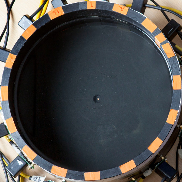
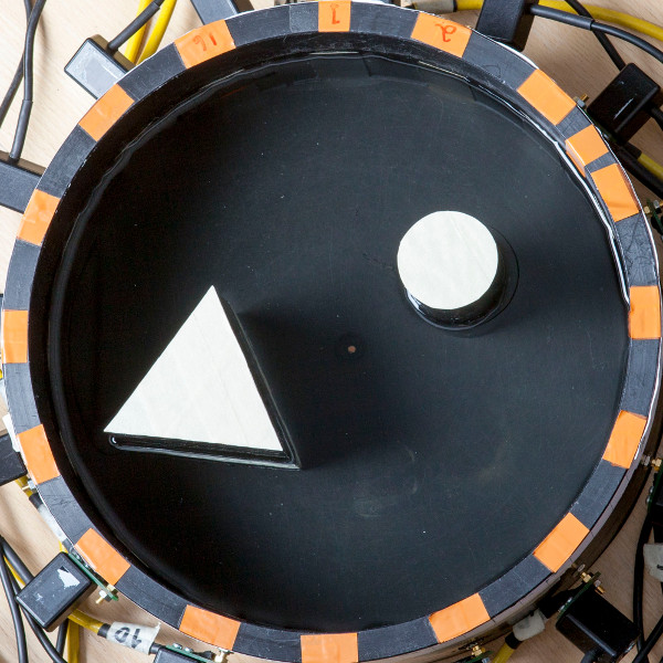
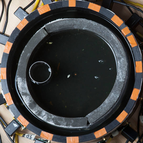
The purpose of this project is to disseminate EIT measurement data from simple experimental setups for the use of testing and development of image reconstruction methods. The experiments were carried out using a flat cylindrical tank filled with saline. Electrically conductive and resistive inclusions were inserted inside the tank, so that they extended from the bottom of the tank to the saline top surface (For two examples, see Figure 1(b).). As also the electrodes on the inner surface of the tank extended from top to bottom, the geometry was essentially two-dimensional (2D) and the measurement data is suitable for 2D EIT.
The rest of this report is organized as follows. In Section 2, we briefly describe the EIT measurements and the target objects used in the experiments. In Section 3, we provide instructions for downloading the Open EIT data, and briefly describe the contents of the data files. Finally, in Section 4, we show example reconstructions computed based on the data.
2 Test cases and data collection
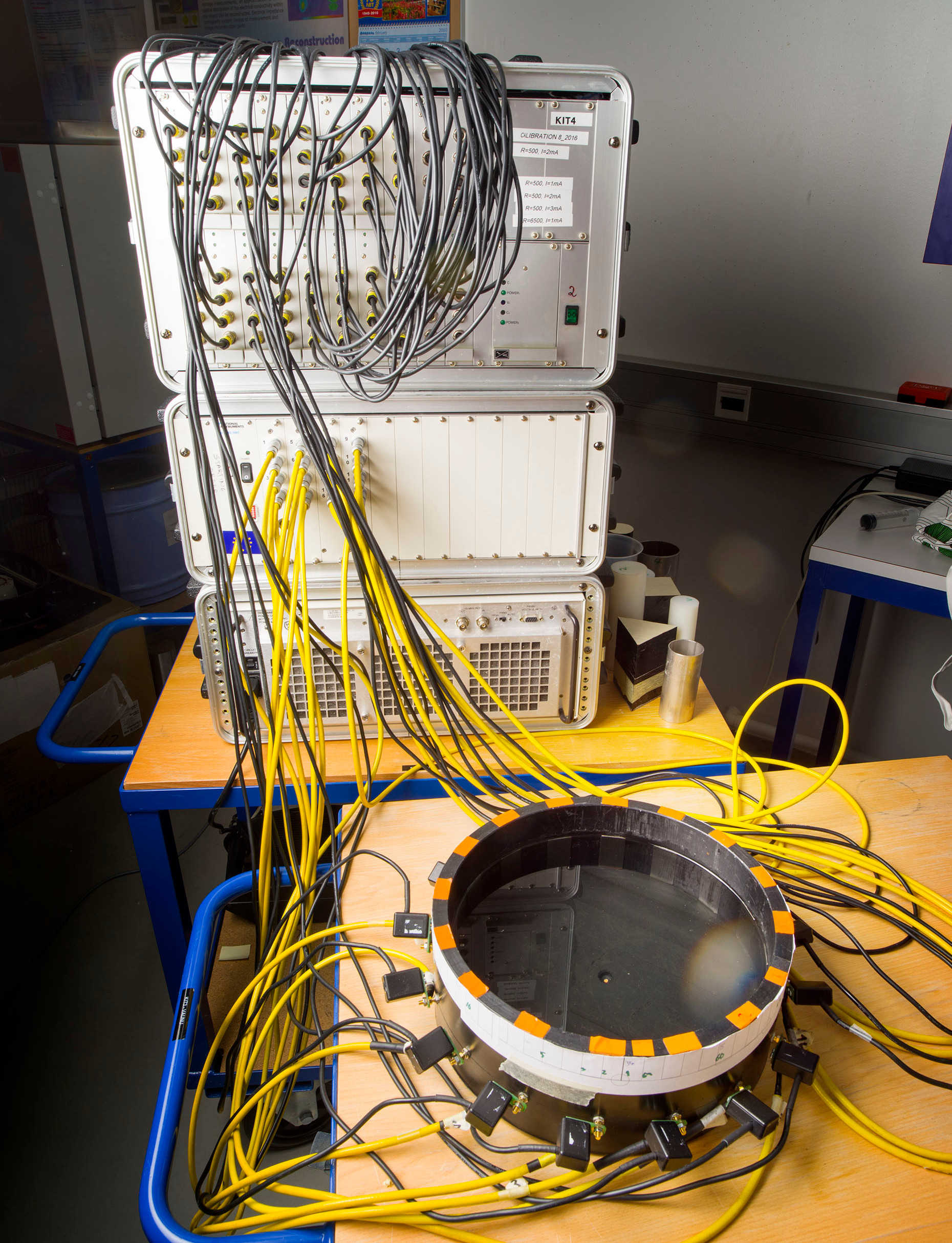
The EIT data set was measured using the KIT4 (Kuopio Impedance Tomography) measurement system (Figure 2). The system consists of three parts. The top part shown in the figure is the voltage measurement module with channels. Up to voltage signals can be simultaneously transferred from the electrodes to the module through the black cables. The middle part is the current injection module with independent current injection channels connected with electrodes via the yellow cables. The lowest part is the controller module. The reader is referred to [2] for detailed description of the KIT4 system.
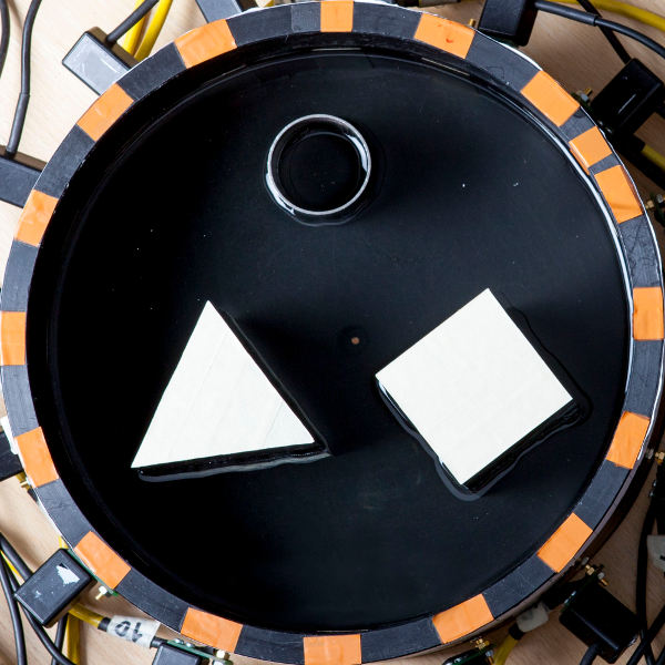
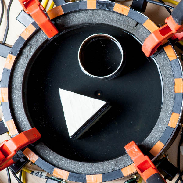
The experiments were conducted using a tank of circular cylinder shape. The diameter of the tank was cm. Sixteen rectangular electrodes (height cm, width cm) made of stainless steel were attached equidistantly on the inner surface of the tank. The electrodes were marked with orange tapes on the tank wall, and they were numbered in clockwise order, see Figure 1(b). In this and in the remaining figures of this document, the topmost electrode is labeled as Electrode .
The tank was filled with saline up to the height of 7 cm, i.e., to the top level of the electrodes. The measured value of the conductivity was S and temperature was °C. Various inclusions were added to the tank in the set of experiments. These inclusions are briefly described along their photographs in Figures 3 – 8.
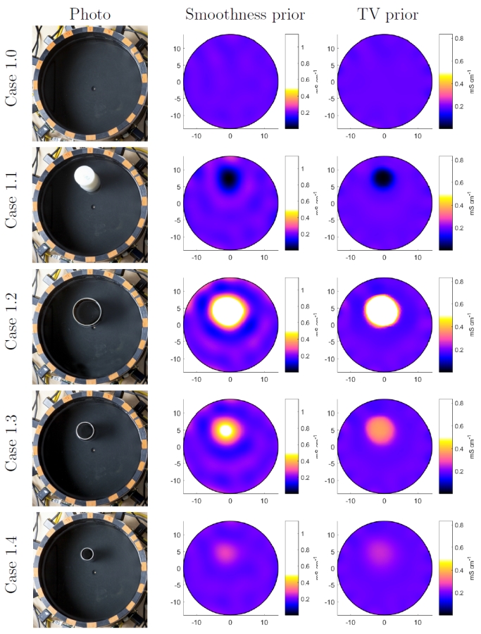
Case 1.0: Homogeneous target
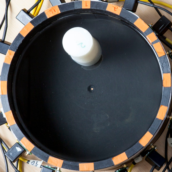
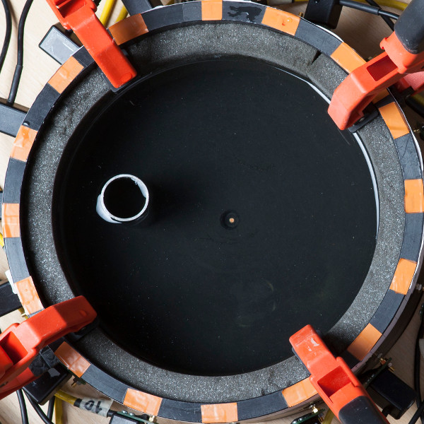
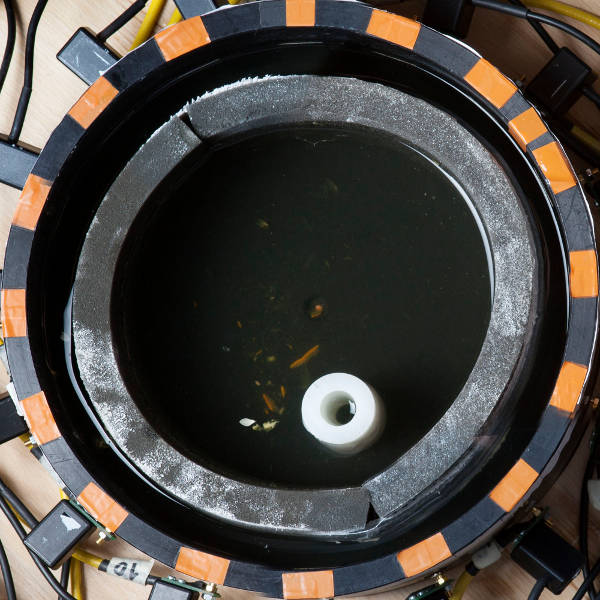
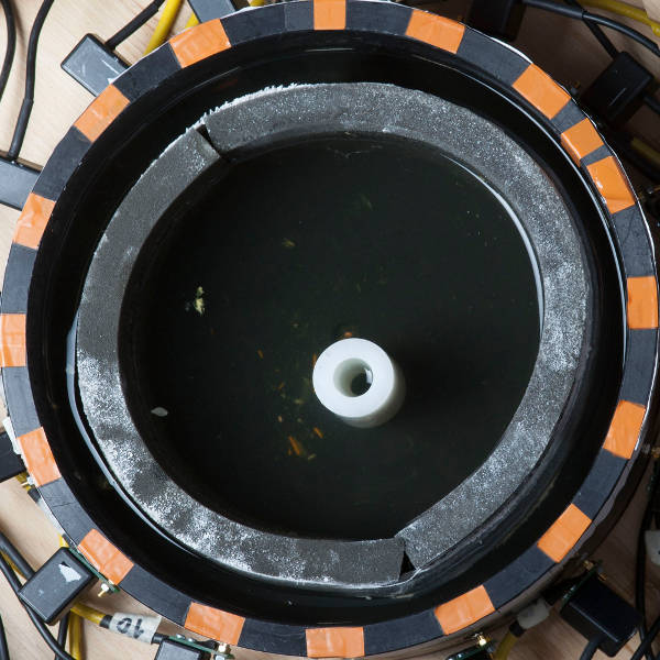
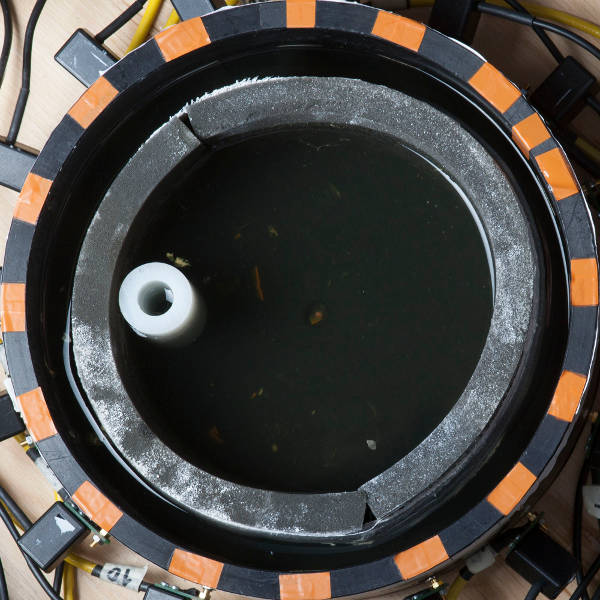
Case 1.1: 1 plastic inclusion (circular)
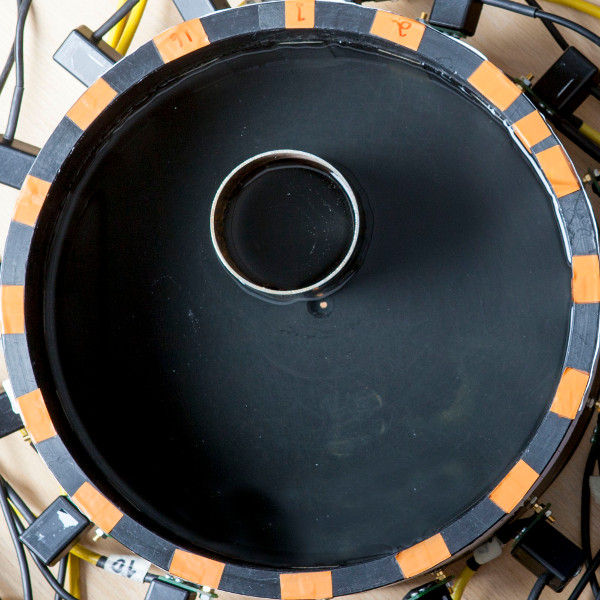
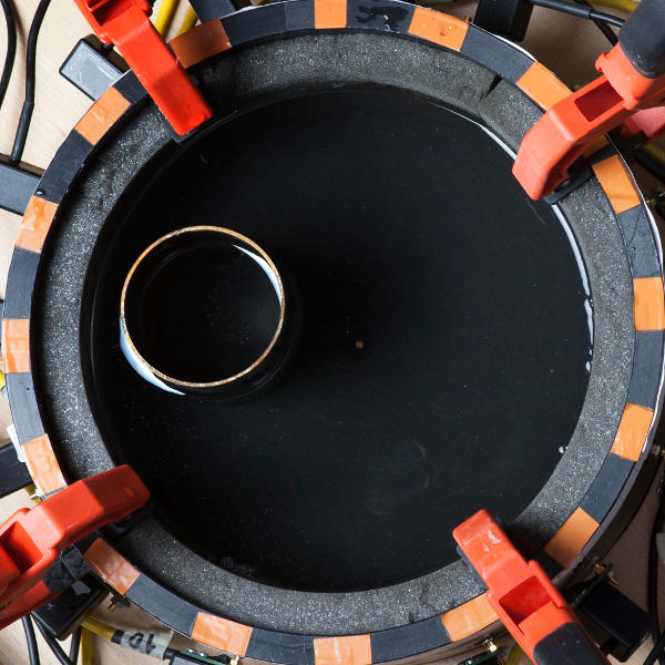
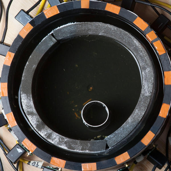
Case 1.2: 1 metallic inclusion (circular, hollow)
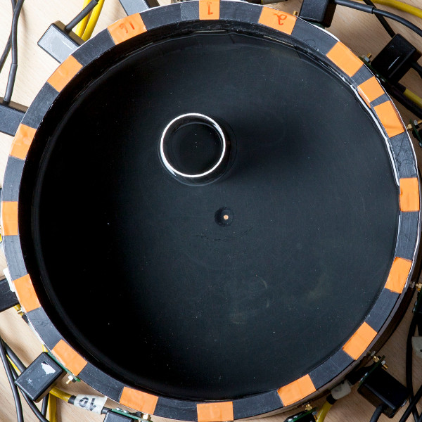
Case 1.3: 1 metallic inclusion (circular, hollow)
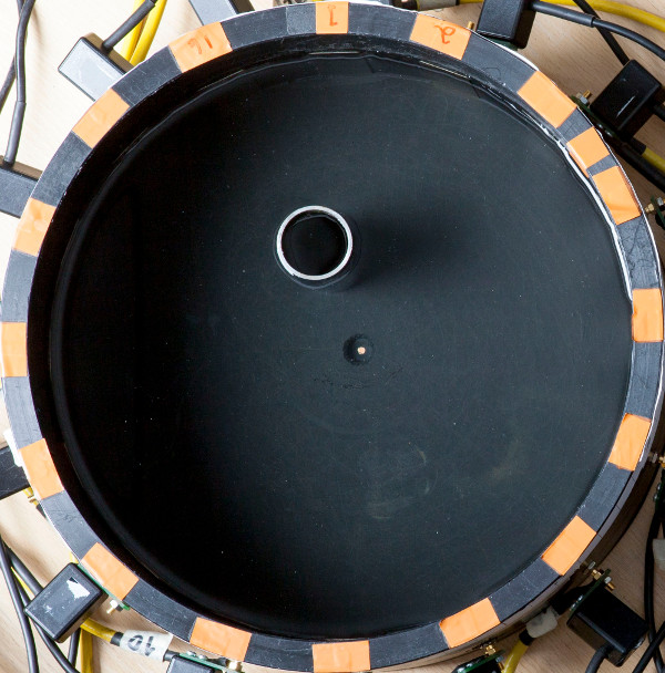
Case 1.4: 1 metallic inclusion (circular, hollow)
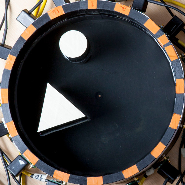
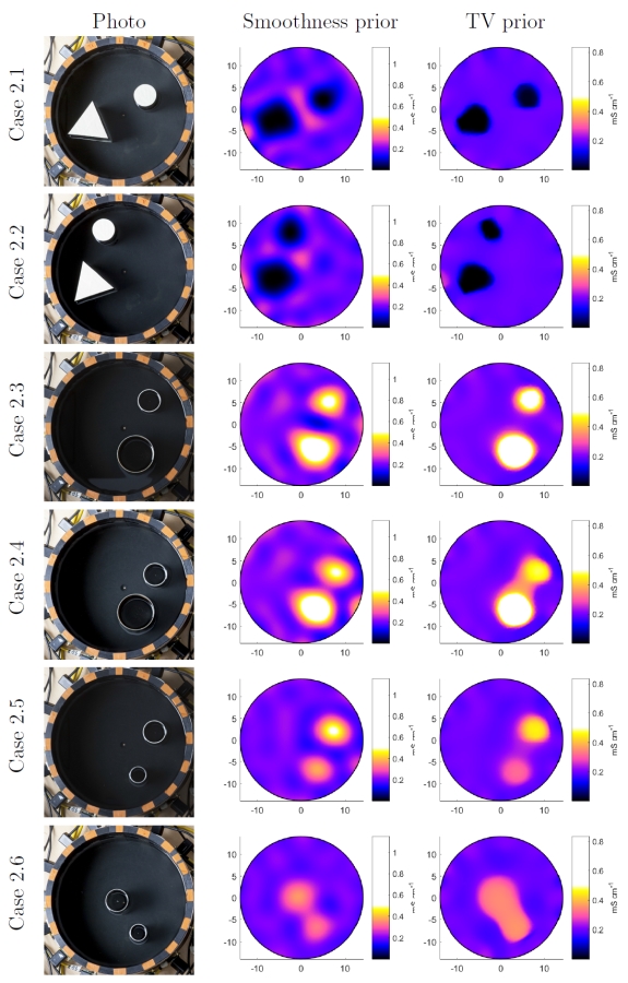
Case 2.1: 2 plastic inclusions (triangular & circular)
Case 2.2: 2 plastic inclusions (triangular & circular)
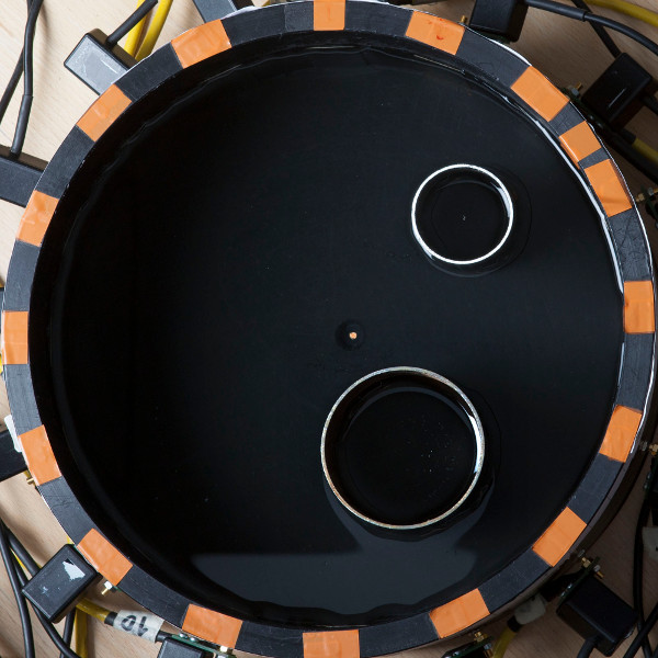
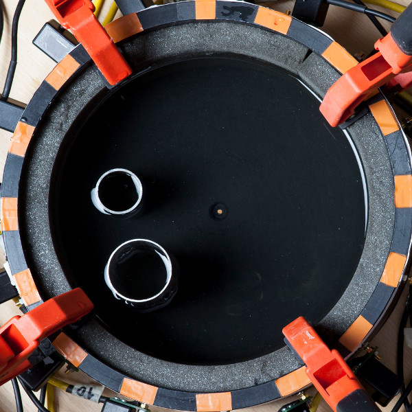
Case 2.3: 2 metallic inclusions (circular, hollow)
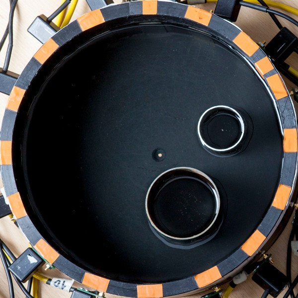
Case 2.4: 2 metallic inclusions (circular, hollow)
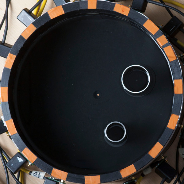
Case 2.5: 2 metallic inclusions (circular, hollow)
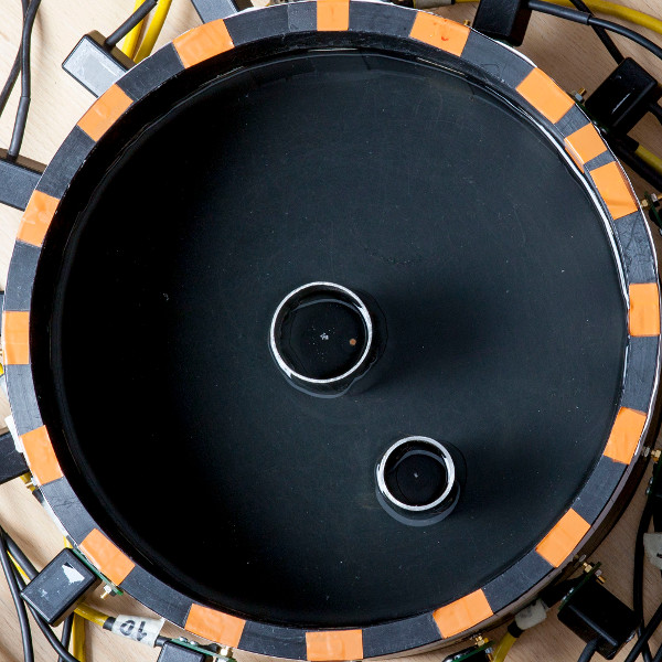
Case 2.6: 2 metallic inclusions (circular, hollow)
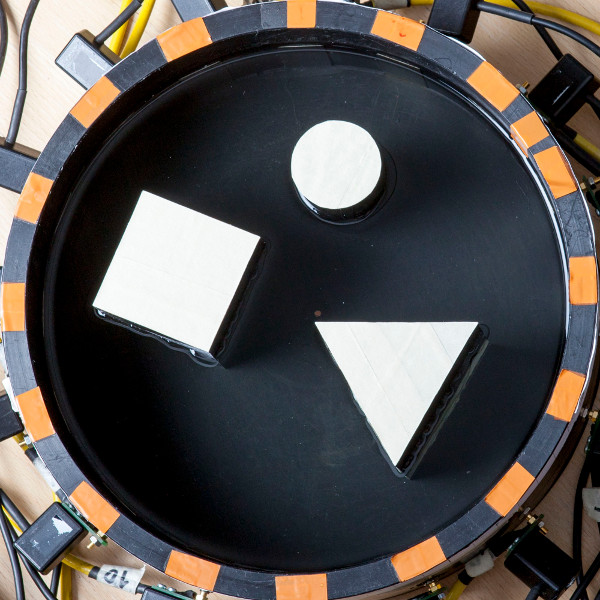
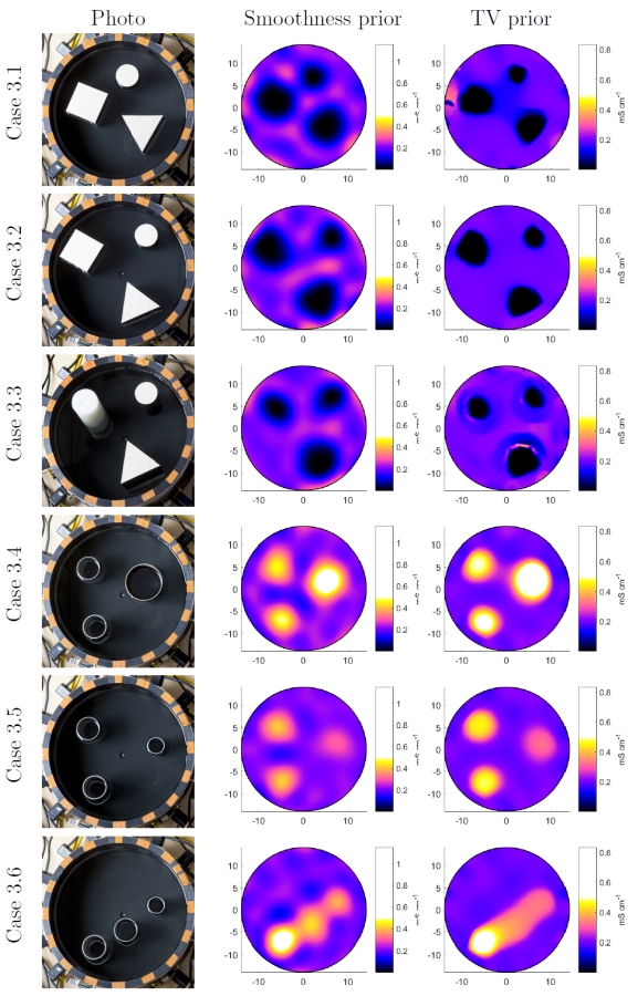
Case 3.1: 3 plastic inclusions (rectangular, triangular & circular)
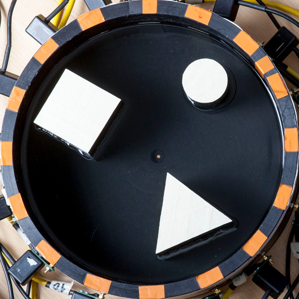
Case 3.2: 3 plastic inclusions (rectangular, triangular & circular)

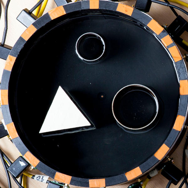
Case 3.3: 3 plastic inclusions (triangular & 2 circular)
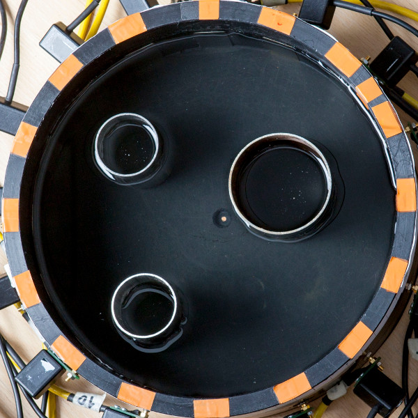
Case 3.4: 3 metallic inclusions (circular, hollow)
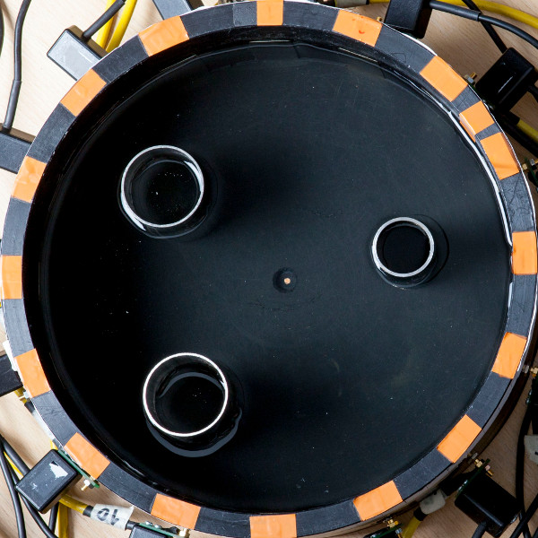
Case 3.5: 3 metallic inclusions (circular, hollow)
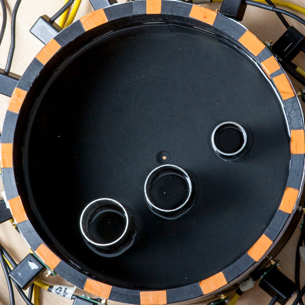
Case 3.6: 3 metallic inclusions (circular, hollow)
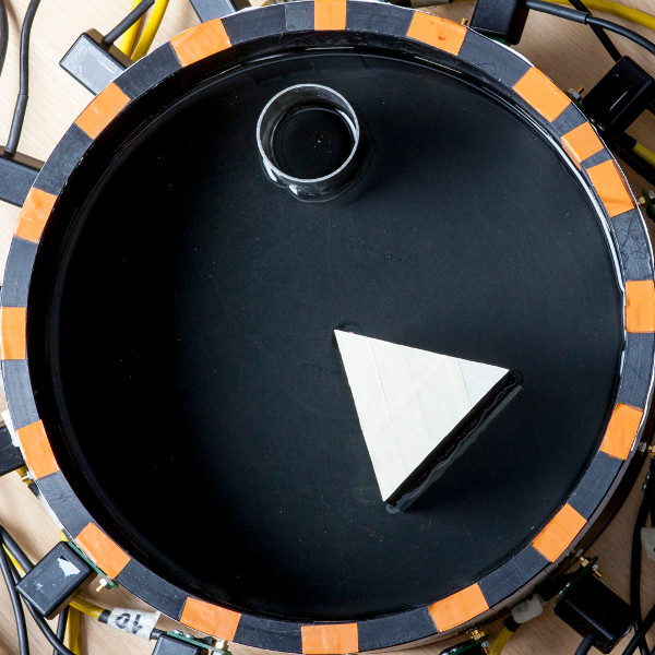
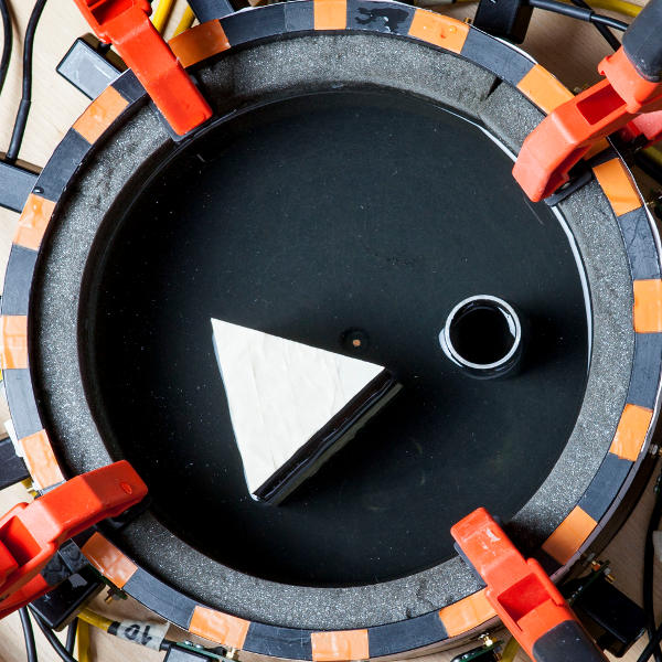
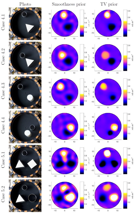
Case 4.1: metallic (circular, hollow) and plastic (triangular) inclusion

Case 4.2: metallic (circular, hollow) and plastic (triangular) inclusion
Case 4.3: metallic (circular, hollow) and plastic (circular) inclusion
Case 4.4: metallic (circular, hollow) and plastic (circular) inclusion
Case 5.1: metallic (circular, hollow) and 2 plastic (triangular and rectangular) inclusions
Case 5.2: 2 metallic (circular, hollow) and 1 plastic (triangular) inclusion
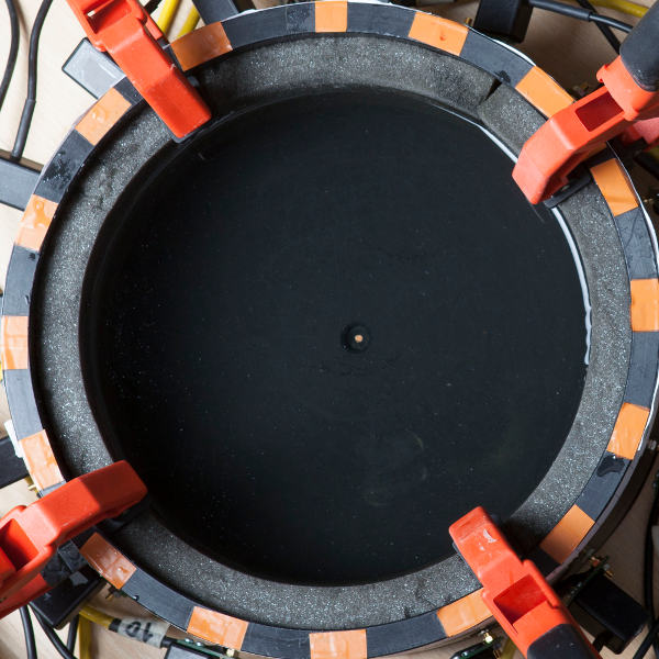
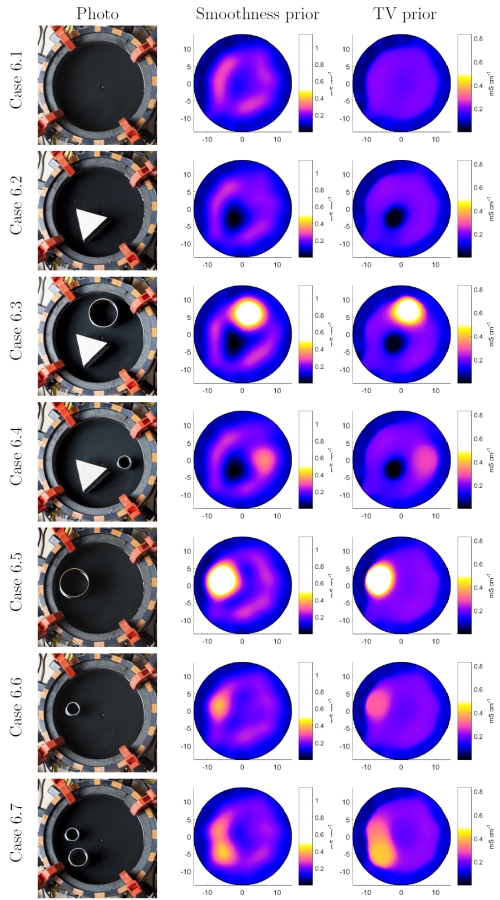
Case 6.1: Annular foam layer on the boundary
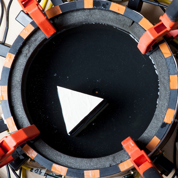
Case 6.2: Foam on the boundary. Plastic inclusion (triangular)
Case 6.3: Foam on the boundary. Plastic (triangular) and metallic (circular, hollow) inclusion
Case 6.4: Foam on the boundary. Plastic (triangular) and metallic (circular, hollow) inclusion
Case 6.5: Foam on the boundary. Metallic (circular, hollow) inclusion
Case 6.6: Foam on the boundary. Metallic (circular, hollow) inclusion
Case 6.7: Foam on the boundary. 2 metallic (circular, hollow) inclusions
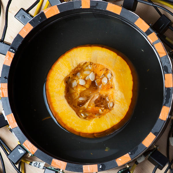
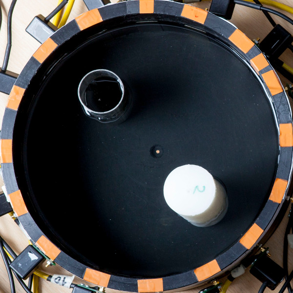
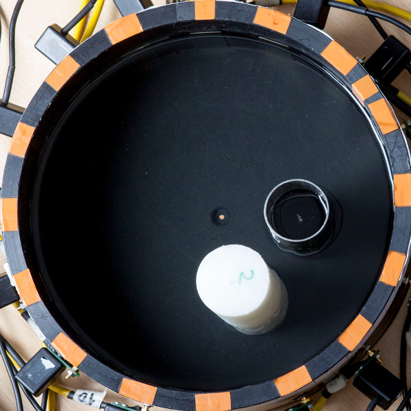
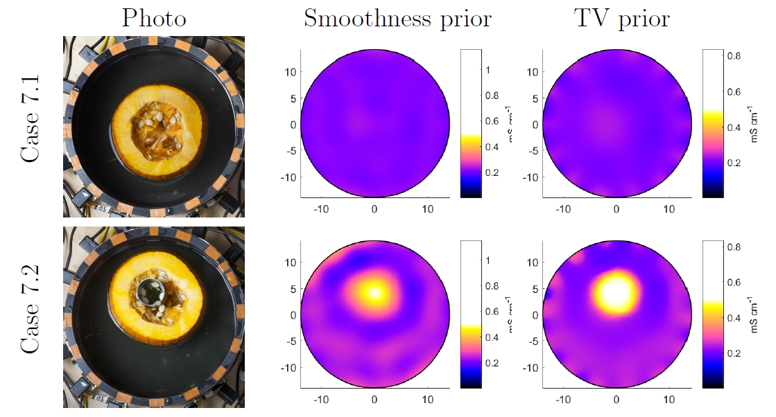
Case 7.1: Slice of pumpkin
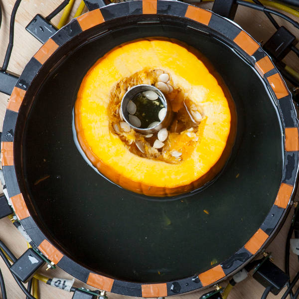
Case 7.2: Slice of pumpkin and metallic inclusion (circular, hollow) inside it
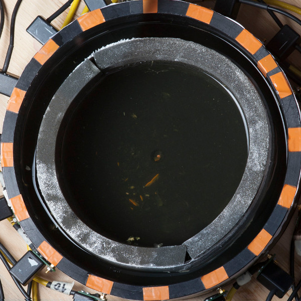
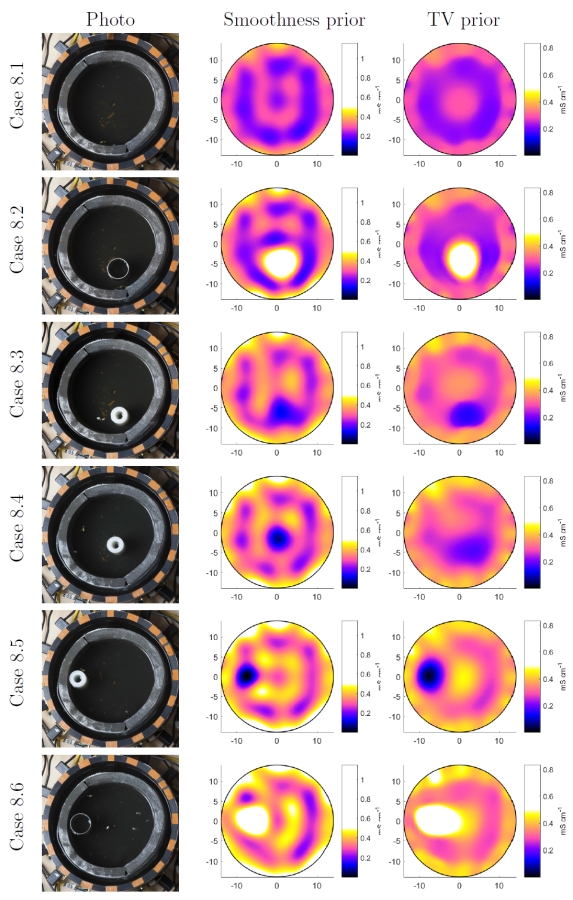
Case 8.1: Annular foam near the boundary
Case 8.2: Foam near boundary, metallic (circular, hollow) inclusion
Case 8.3: Foam near boundary, plastic (circular, hollow) inclusion
Case 8.4: Foam near boundary, plastic (circular, hollow) inclusion
Case 8.5: Foam near boundary, plastic (circular, hollow) inclusion
Case 8.6: Foam near boundary, metallic (circular, hollow) inclusion
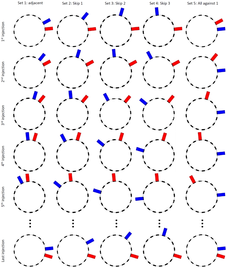
For the EIT measurements, a total of pairwise current injections were used. The injected currents can be divided into five sets:
-
•
Set 1: Adjacent injections. Injections between electrodes 1-2, 2-3,,15-16, 16-1.
-
•
Set 2: Skip 1. Injections between electrodes 1-3, 2-4,,14-16, 15-1, 16-2.
-
•
Set 3: Skip 2. Injections between electrodes 1-4, 2-5,,13-16, 14-1, , 16-3.
-
•
Set 4: Skip 3. Injections between electrodes 1-5, 2-6,,12-16, 13-1, , 16-4.
-
•
Set 5: All against 1. Injections between electrodes -1, where the .
Here, the first electrode in the electrode pair - refers to the electrode carrying a positive current and the second electrode carries the negative current. The current injections are illustrated in Figure 9.
The amplitudes of the currents were mA and their frequencies were 1 kHz. Corresponding to each current injection, voltages were measured between all adjacent electrodes: 1-2, 2-3,,15-16, 16-1, resulting in total of 7916 =1264 measurements.
3 Contents of the data set
To use Open 2D EIT data, download and extract the following compressed folders:
-
•
Measurements: fips.fi/EIT_data/data_mat_files.zip
-
•
Photographs: fips.fi/EIT_data/target_photos.zip
These folders contain, respectively, data files and photographs named as
-
•
datamatXY.mat
-
•
fantomXY.jpg
where the indices and refer to numbers of the experiments (cf. Figures 3 – 8). For example, datamat12.mat stores EIT measurements of Case and fantom12.jpg is a photo of this experiment.
Each data file datamatXY.mat contains the following matrices:
-
•
Uel : voltage measurements (each column consist of 16 adjacent voltage measurements corresponding to one current injection).
-
•
CurrentPattern : current patterns (each column defines the currents on 16 electrodes in one current injection).
-
•
MeasPattern : measurement patterns (each column defines the measuring electrodes in the corresponding voltage measurement).
A brief Matlab code for reading the data files is provided in link http://fips.fi/EIT_data/LoadData.m. For examples of selecting only parts of data (e.g., measurements corresponding to any of the current injection sets in Figure 9) we refer to comments in the m-file.
Finally, we would like to remind the readers to kindly cite this document whenever using any part of the Open 2D EIT data in a publication.
4 Example reconstructions
To illustrate the use of the data, we computed EIT reconstructions of all targets. In Figures 10 – 16, the photograph of each target is accompanied with two example reconstructions: one using a smoothness promoting prior/regularization [3] and one using isotropic TV prior [1]. All these reconstructions were computed using absolute imaging, i.e., no reference data from the case of homogeneous target was used in the reconstructions of inhomogeneous conductivity distributions. For modeling the measurements, a three-dimensional (3D) finite element based forward model was used [4]; however, as all targets were known to be (at least approximately) constant along the vertical direction, the conductivity distribution was parametrized in 2D. Further, as contact impedances between the electrodes and the saline were unknown, they were estimated simultaneously with the conductivity in each reconstruction [5]. We also note that all reconstructions corresponding to each reconstruction method were computed using the same choices of parameters in the models, and in Figures 10 – 16, all images corresponding to each reconstruction method are represented in mutually equal color scale. As the purpose of the reconstructions is only to demonstrate the feasibility of the measurement data, we omit the details of the reconstruction methods here. For details, we refer to the papers cited above.
All inclusions in the phantoms are tracked with both reconstruction methods. In the locations of electrically resistive inclusions, the reconstructed conductivity is close to zero (indicated by black color), and in the locations of the highly conductive objects, the reconstructed conductivity is higher than the background conductivity (colors ranging from magenta to white). We note here that the top of the color scale is specifically chosen (wide range of conductivities marked with white) for the purpose of illustrating all reconstructions – featuring both positive and negative changes from the background conductivity – in the same color scale. The sensitivity of EIT to the magnitude of the positive conductivity change from the background decreases after certain limit, and consequently in Figures 10 – 16, the reconstructed values in the "white range" ( mS/cm) possess high uncertainty.
References
- [1] G. Gonzalez, J. Huttunen, V. Kolehmainen, A. Seppänen, and M. Vauhkonen. Experimental evaluation of 3d electrical impedance tomography with total variation prior. Inverse Problems in Science and Engineering, 24(8):1411–1431, 2016.
- [2] J. Kourunen, T. Savolainen, A. Lehikoinen, M. Vauhkonen, and L. Heikkinen. Suitability of a PXI platform for an electrical impedance tomography system. Measurement Science and Technology, 20(1):015503, 2008.
- [3] A. Lipponen, A. Seppänen, and J. Kaipio. Electrical impedance tomography imaging with reduced-order model based on proper orthogonal decomposition. Journal of Electronic Imaging, 22(2):023008–023008, 2013.
- [4] P. J. Vauhkonen, M. Vauhkonen, T. Savolainen, and J. P. Kaipio. Three-dimensional electrical impedance tomography based on the complete electrode model. IEEE Transactions on Biomedical Engineering, 46(9):1150–1160, 1999.
- [5] T. Vilhunen, J. Kaipio, P. Vauhkonen, T. Savolainen, and M. Vauhkonen. Simultaneous reconstruction of electrode contact impedances and internal electrical properties: I. theory. Measurement Science and Technology, 13(12):1848, 2002.
Andreas Hauptmann, Department of Mathematics and Statistics, University of Helsinki, Finland
E-mail address: andreas.hauptmann@helsinki.fi
Ville Kolehmainen, Department of Applied Physics, University of Eastern Finland
E-mail address: ville.kolehmainen@uef.fi
Nguyet Minh Mach, Department of Mathematics and Statistics, University of Helsinki, Finland
E-mail address: minh.mach@helsinki.fi
Tuomo Savolainen, Department of Applied Physics, University of Eastern Finland
E-mail address: tuomo.savolainen@uef.fi
Aku Seppänen, Department of Applied Physics, University of Eastern Finland
E-mail address: aku.seppanen@uef.fi
Samuli Siltanen, Department of Mathematics and Statistics, University of Helsinki, Finland
E-mail address: samuli.siltanen@helsinki.fi