Bound state energies using Phase integral methods

Abstract

The study of asymptotic properties of solutions to differential equations has a long and arduous history, with the most significant advances having been made in the development of quantum mechanics. A very powerful method of analysis is that of Phase Integrals, described by Heading. Key to this analysis are the Stokes constants and the rules for analytic continuation of an asymptotic solution through the complex plane. These constants are easily determined for isolated singular points, by analytically continuing around them and, in the case of analytic functions, requiring the asymptotic solution to be single valued. However, most interesting problems of mathematical physics involve several singular points. By examination of analytically tractable problems and more complex bound state problems involving multiple singular points, we show that the method of Phase Integrals can greatly improve the determination of bound state energy over the simple WKB values. We also find from these examples that in the limit of large separation the Stokes constant for a first order singular point approaches the isolated singular point value.

I introduction

Many differential equations of interest can be put in the form

$$\frac{d^{2}\psi}{dz^{2}}+Q(z,E)\psi=0.$$ (1)

For bound state problems the existence of solutions and the energy eigenvalue $E$ can often be determined by Phase Integral methods. Briefly, the WKBJ (and often simply WKB) approximate solutions of Eq. 1, so named after Wentzel, Kramers, Brillouin, and Jeffreyswkbj , take the form

$$\psi_{\pm}=Q^{-1/4}e^{\pm i\int^{z}Q^{1/2}dz},$$ (2)

and provided that $\left|\frac{dQ}{dz}Q^{-3/2}\right|\ll 1$ a general solution of Eq. 1 can be approximated by

$$\psi=a_{+}\psi_{+}+a_{-}\psi_{-}.$$ (3)

The solutions $\psi_{\pm}$ are local, not global solutions of Eq. 1. Clearly the inequality is not valid in the vicinity of a zero of $Q(z,E)$, commonly called a turning point. Aside from this, however, $\psi_{\pm}$ are not approximations of a continuous solution of Eq. 1 in the whole z plane. The method of Phase Integrals, described by Headingheading , but first suggested by A. Zwann in his dissertation in 1929, consists in relating, for a given solution of Eq. 1, the WKBJ approximation in one region of the $z$ plane to that in anotherrwbook ; rwnum . The solution then gives an approximation to the global solution of the given differential equation. The WKB approximation has an extensive application in quantum mechanics and other branches of physics, along with many attempts to improve its accuracydunham ; dingle73 ; berry90 ; berry91 ; sergeenko96 ; delabaere97 ; sergeenko02 ; mirnov10 ; poor16 .

The regions in the complex plane defining the validity of the individual approximations to the solution are separated by the so-called Stokes and anti-Stokes lines associated with $Q(z,\omega)$, and thus the qualitative properties of the solution are determined once these lines are known. The global Stokes (anti-Stokes) lines associated with $Q(z,\omega)$ are paths in the $z$ plane, emanating from zeros or singularities of $Q(z,\omega)$, along which $\int Q^{1/2}(z,\omega)dz$ is imaginary (real). When the zero $z_{0}$ is first order, three anti-Stokes lines emanate from $z_{0}$. Similarly, one finds that from a double root there issue four anti-Stokes lines, from a simple pole a single line, etc.. In refering to Stokes diagrams, we will refer to both zeros and singularities of Q(z) as singular points, since it is the function $Q^{1/2}$ which is relevant in this diagram.

Along the global anti-Stokes lines the functions $\psi_{\pm}$ are, within the validity of the WKBJ approximation, of constant amplitude, $i.e.$ oscillatory. Along the Stokes lines the WKBJ solutions are exponentially increasing or decreasing with fixed phase. Except at singular points, the Stokes and anti-Stokes lines are orthogonal. The global anti-Stokes and Stokes lines which are attached to the singular points of the Stokes diagram, along with the Riemann cut lines, determine the global properties of the WKBJ solutions.

In the notation of Heading, including the slow $Q^{-1/4}$ dependence, a WKBJ solution is denoted by

$$(a,z)_{s}=Q^{-1/4}e^{i\int_{a}^{z}Q^{1/2}dz}$$ (4)

where the subscript s(d) indicates that the solution is subdominant (dominant); $i.e.$ exponentially decreasing (increasing) for increasing $|z-a|$ in a particular region of the $z$ plane, bounded by Stokes and anti-Stokes lines.

Begin with a particular solution in one region of the $z$ plane, choosing that combination of subdominant and dominant solutions which gives the desired boundary conditions in this region. The global solution is obtained by continuing this solution through the whole $z$ plane effecting the following changes due to the monodromy of the WKB solutionspoor16 moving through the plane:

1. Given a solution $\psi=a_{d}(z_{0},z)_{d}+a_{s}(z,z_{0})_{s}$, upon crossing a Stokes line emanating from $z_{0}$ in a counterclockwise sense $a_{s}$ must be replaced by $a_{s}+Sa_{d}$ where S is the Stokes constant associated with $z_{0}$.

2. Upon crossing a cut in a counterclockwise sense, the cut originating from a first order zero of $Q$ at the point $z_{0}$, we have

$$(z_{0},z)\rightarrow-i(z,z_{0})$$

$$(z,z_{0})\rightarrow-i(z_{0},z).$$ (5)

Properties of dominancy or subdominancy are preserved in this process.

3. Upon crossing an anti-Stokes line emanating from $z_{0}$, subdominant solutions attached to $z_{0}$ become dominant and vice versa.

4. Reconnect from singularity $a$ to singularity $b$ using $(z,a)=(z,b)[b,a]$ with $[b,a]=e^{i\int_{b}^{a}Q^{1/2}dz}$.

Using these rules we can pass from region to region across the cuts, Stokes and anti-Stokes lines emanating from the singularities. Beginning with any combination of dominant and subdominant solutions in one region, this process leads to a globally defined approximate solution of Eq. 1.

For an isolated singular point with $Q$ analytic, the Stokes constant can be determined by a continuation around the complex plane, requiring that the WKB approximation be single valued. This gives for $Q=z^{n}$, the value $S=2icos(\pi/(n+2))$.

Any function given on the real axis can be analytically continued into the complex plane, resulting in a collection of zeros and singularities associated with the functional form on the axis. Every bound state problem consists of two turning points, with the potential positive outside them, and negative inside. The simplest bound state problem, the harmonic oscillator, given by the Weber equation with $Q=E-z^{2}$, is unique in that there are no additional zeros or singularities in the complex plane, the function is completely described by the zeros on the real axis. For this case the energy of the bound state as well as the single valuedness of the solution turn out to be independent of the value of the Stokes constant but the equation can be solved analytically, giving the Stokes constant for any energy.

In section II we review this case. In section III we examine the Budden problem, another case with two singular points which admits an analytic solution. In sections IV and V we consider Hermitian anharmonic oscillator Hamiltonians with additional zeros above and below the axis, and in section VI we consider a non-Hermitian Hamiltonian with three singular points. The shape of these potentials is shown is section VII. Finally in section VIII are the conclusions.

II The Weber function

The simplest bound state problem is given by the harmonic oscillator potential, with $Q(z)=E-z^{2}$, real on the real axis with two first order zeros at points $\pm\sqrt{E}$. The Stokes diagram is shown in Fig. 1. The solid lines are Anti Stokes lines, dashed lines are Stokes lines, and cuts are designated with a wavy line. It is important to note that the results of any calcuation are independent of the location of the Riemann cuts, so they can be placed to be convenient for a given calculation. Denoting the Stokes constant as $S$, we will find that the boundary conditions immediately give the Bohr–Sommerfeld condition, which determines the energy of the bound state, independent of the value of the Stokes constant.

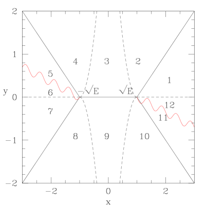
Figure 1: Stokes plot for the bound state problem $Q=E-z^{2}$.

Begin with a subdominant solution at large positive $x$ and continue, assuming Stokes constants the same at each vertex, with $a=\sqrt{E}$:
(1) $(a,z)_{s}$
(2) $(a,z)_{d}$
(3) $(a,z)_{d}+S(z,a)_{s}$
(3) $[a,-a](-a,z)_{d}+S(z,-a)_{s}[-a,a]$
But $[-a,a]=e^{-iW}$, $W=\int_{-a}^{a}\sqrt{a^{2}-x^{2}}dx$. Note that the phase of $\sqrt{Q}$ is defined by requiring that $(a,z)_{s}$ be subdomanant in domain 1, so $i\sqrt{Q}=-real$. The cut locations define the phase in other domains.
(4) $e^{iW}(-a,z)_{d}+S(z,-a)_{s}(e^{-iW}+e^{iW}$)
(5) $e^{iW}(-a,z)_{s}+S(z,-a)_{d}2cosW$
(6) $-ie^{iW}(z,-a)_{s}-iS(-a,z)_{d}2cosW$
Now set the dominant term to zero giving $W=(n+1/2)\pi$, the Bohr Sommerfeld condition, independent of the value of the Stokes constant. Note that $-ie^{iW}=(-1)^{n}$, the coefficient correctly reflects even and odd symmetry of the solution. Continuing around to domain (12)
(7) $-ie^{iW}(z,-a)_{s}$
(8) $-ie^{iW}(z,-a)_{d}$
(9) $-ie^{iW}[(z,-a)_{d}+S(-a,z)_{s}]$
(9) $-ie^{iW}[(z,a)_{d}[a,-a]+S[-a,a](a,z)_{s}]$
(9) $-ie^{2iW}(z,a)_{d}-iS(a,z)_{s}$
(10) $i(z,a)_{d}$
(11) $i(z,a)_{s}$
(12) $(a,z)_{s}$,
we find again a subdominant solution with coefficient equal to one, so the solution is single valued, independent of the value of S provided that the Bohr-Sommerfeld condition on the energy is satisfied. Of course every Stokes constant has a definite value, which can be revealed from an exact solution.

A general solution of the Weber equation can be written with use of parabolic cylinder functions:

$$y(z)=C_{1}U(-E/2,\sqrt{2}z)+C_{2}U(E/2,i\sqrt{2}z).$$ (6)

To find Stokes constants in the upper half-plane of the complex z-plane let us choose $C_{1}$ and $C_{2}$ such that $y(z)\sim(a,z)$ for $-\pi/4<Arg(z)<\pi/4$. According to Eq. 4

$$(a,z)=(E-z^{2})^{-1/4}e^{i\int_{a}^{z}(E-z^{2})^{1/2}dz}=(E-z^{2})^{-1/4}e^{-z^{2}/2+E/4+(E/2)\ln{(2z/\sqrt{E})}+O(1/z)},$$ (7)

and in a limit of large $z$ we can write

$$(a,z)\sim e^{i\pi/4}\left(2\sqrt{\frac{e}{E}}\right)^{E/2}z^{-1/2+E/2}e^{-z^{2}/2},$$ (8)

$$(z,a)\sim e^{i\pi/4}\left(2\sqrt{\frac{e}{E}}\right)^{-E/2}z^{-1/2-E/2}e^{z^{2}/2}.$$ (9)

The common factor $e^{i\pi/4}$ can be omitted for further calculations due to the linearity of the Weber equation.

Using asymptotic expansions for the parabolic cylinder functions we find that the required values for the arbitrary constants are

$$C_{1}=2^{-1/4}(2e/E)^{-E/4},C_{2}=0.$$ (10)

Once we have determined the values of the arbitrary constants in Eq.6, we can write an asymptotic expansion of our solution in any domain. Particularly, for $\pi/4<Arg(z)<3\pi/4$ it has the form

$$y(x)\sim(a,z)_{d}+i\frac{\sqrt{2\pi}e^{i\pi E/2}}{\Gamma(\frac{1-E}{2})}(2e/E)^{E/2}(z,a)_{s}.$$ (11)

Now compare this relation with the one from the WKB analysis performed above, line $4$. One might think that the coefficient of the subdominant function is equal to $S(e^{-iW}+e^{iW})$ but this is not quite true. Since Stokes constants depend on the lower limit of integration used in the WKB-approximation we should at first write everything in a unique base and only then compare rigorous result with the WKB one. And since $(a,z)=[a,-a](-a,z)$ and $(z,a)=(z,-a)[-a,a]$ we can write

$$S(1+e^{2iW})=i\frac{\sqrt{2\pi}e^{i\pi E/2}}{\Gamma(\frac{1-E}{2})}(2e/E)^{E/2}.$$ (12)

As long as we chose a branch of the square root such that $(a,z)$ is subdominant for large positive z, $W=\pi E/2$ and

$$S=i\frac{\sqrt{2\pi}e^{i\pi E/2}}{\Gamma(\frac{1-E}{2})}(2e/E)^{E/2}(1+e^{i\pi E})^{-1}.$$ (13)

Now one can easily see that $S$ approaches $i$ for large energies.

Figure 2: Thedifference between $i$ and the actual value of the Stokes constant for the Weber equation

III The Budden equation

Another example of a potential which allows exact calculation of Stokes constants is the Budden potential with $Q(z)=1+c/z$. We will see that the Stokes constants approach $i$ for large values of $c$ exactly as in the previous chapter.

Figure 3: Stokes plot for the Budden problem $Q=1+c/z$.

Before we calculate Stokes constants let us perform a WKB analysis. Choosing zero as a lower limit of integration we have

$$i\int_{0}^{z}\sqrt{1+\frac{c}{x}}dx=iz+\frac{ic}{2}-\frac{ic}{2}\ln{\left(\frac{c}{4z}\right)}+O\left(\frac{1}{\sqrt{z}}\right)$$ (14)

and in a limit of large z

$$(0,z)\sim\left(\frac{4e}{c}\right)^{ic/2}z^{ic/2}e^{iz},$$ (15)

$$(z,0)\sim\left(\frac{4e}{c}\right)^{-ic/2}z^{-ic/2}e^{-iz}.$$ (16)

To perform an analytical continuation around the origin, place the cut between $z=0$ and $z=-c$ along the real axis as shown in Fig.3. Starting with $y(z)\sim(0,z)$ at large negative $z$ and using the rules of a continuation, one finds that the continuation is
$3.\ (0,z)_{d}=[0,-c](-c,z)_{d}$
$2.\ [0,-c](-c,z)_{d}+S[0,-c](z,-c)_{s}$
$1.\ [0,-c](-c,z)_{s}+S[0,-c](z,-c)_{d}=(0,z)_{d}+S[0,-c]^{2}(z,0)_{s}$
All integrals here were evaluated below the cut and give $[0,-c]=e^{\frac{\pi c}{2}}$.

Now we can find an exact value of $S$. A general solution for the Budden equation is

$$y(z)=ze^{-iz}[C_{1}U(1+\frac{ic}{2},2,2iz)+C_{2}M(1+ic/2,2,2iz)],$$ (17)

where $U(a,b,z)$ and $M(a,b,z)$ are Kummer functions. Requiring the solution $y(z)$ to be asymptotic to $(0,z)$ for large negative $z$ we find that

$$C_{1}=\frac{\Gamma(1+\frac{ic}{2})}{\Gamma(1-\frac{ic}{2})}e^{3\pi c/4}\left(\frac{2e}{c}\right)^{ic/2},$$ (18)

$$C_{2}=\Gamma(1+\frac{ic}{2})e^{\pi c/4}\left(\frac{2e}{c}\right)^{ic/2}.$$ (19)

Now, using an asymptotic expansion of this solution for large positive z we have

$$y(z)\sim(0,z)+\frac{\Gamma(1+\frac{ic}{2})}{\Gamma(1-\frac{ic}{2})}\left(\frac{2e}{c}\right)^{ic}(e^{\pi c}-1)(z,0).$$ (20)

Finally, comparing this asymptotic relation with the one from our WKB analysis we deduce that

$$S=\frac{\Gamma(1+\frac{ic}{2})}{\Gamma(1-\frac{ic}{2})}(\frac{2e}{c})^{ic}(1-e^{-\pi c}).$$ (21)

It can be easily verified that this Stokes constant approaches $i$ for large values of $c$, as shown in Fig. 4.

Figure 4: The difference between $i$ and actual value of Stokes constant for the Budden equation

IV A fourth order potential

Now consider a more complicated potential, that of an anharmonic oscillator, with more turning points in the complex plane. As an example we take $Q(z)=E-z^{4}$. The Stokes structure is shown in Fig. 5. The cuts have been chosen to give symmetry in the continuation between the upper and lower half planes. We assume the Stokes constants to be the same at all singular points. This is probably not true for general separation, but we will be restricted to an asymptotic evaluation for large separation, and this turns out to be true to leading order.

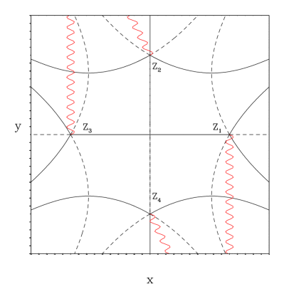
Figure 5: Stokes plot for the bound state problem $Q=E-z^{4}$.

In order to do the connections, we need the expressions $[k,l]=e^{\int_{z_{k}}^{z_{l}}i\sqrt{Q(z)}dz}$. Note that the sheet of $i\sqrt{Q(z)}$ is defined by the cut locations, with the initial sheet determined by the fact that $(z_{1},z)$ is subdominant for $x\rightarrow+\infty$ , meaning that $i\sqrt{Q}(z)=-real$ in this domain.

Carrying out the integrals then gives

$$[1,2]=e^{W/2}e^{iW/2},\hskip 14.22636pt[1,3]=e^{iW},\hskip 14.22636pt[2,3]=e^{-W/2}e^{iW/2}$$ (22)

where $W=E^{3/4}\int_{-1}^{1}\sqrt{1-u^{4}}du$, and $\int_{-1}^{1}\sqrt{1-u^{4}}du=1.74804$.

Begin with a subdominant solution $\psi(z)=(Z_{1},z)_{s}$ at large positive $x$ and continue through the upper half plane above the singularity at $iE^{1/4}$ to large negative $x$. Using the symmetry of the potential we have

$$Se^{-W}+Se^{iW}=-(-1)^{n}.$$ (23)

Also we find a condition for the vanishing of the dominant solution

$$e^{W}[1+S^{2}]+2S^{2}cos(W)+e^{-W}S^{2}=0.$$ (24)

For large turning point separation $W$ is large and we have a solution given by the isolated turning point values, $S=i$ and $W_{n}=(n+1/2)\pi$, the usual approximate WKB solution. There is a natural perturbation expansion parameter given by the existence of the exponential term $e^{-W}$, present because of the additional singular points not on the real axis. Even for the lowest bound state as given by the WKB approximation $e^{-W_{0}}\simeq 0.2$, and for the next level $e^{-W_{1}}\simeq 0.009$.

Perturbing about the WKB value $W_{n}=(n+1/2)\pi$ gives the solution

$$S\simeq i\left[1-cos(W_{n})e^{-W_{n}}-\frac{e^{-2W_{n}}}{2}\right],\hskip 28.45274ptcos(W)=-e^{-W_{n}}.$$ (25)

Thus $S\simeq i(1+e^{-2W}/2)$ and $sin(W)=(-1)^{n}\sqrt{1-cos^{2}(W)}\simeq(-1)^{n}(1-e^{-2W}/2)$, where we have dropped terms of order $e^{-4W}$, amounting to a correction to the ground state energy of a fraction of a percent.

Values of the exact energy levels, the WKB approximation, and the Phase Integral evaluation are shown in table I. For the ground state $E_{PI}$ has a 4 percent error, $E_{WKB}$ has a 20 percent error.

This problem has also been approached using higher order phase integral approximationscampbell ; bender77 . A third order solution using the phase integral series due to Fromanfroman is given in table 2.1 of Childchild . The third order approximation to the ground state eigenvalue is given as 0.98076, with an error over 7 percent.

$${\bf Table\hskip 2.84526ptI.\hskip 5.69054ptEnergy\hskip 5.69054ptLevels\hskip 5.69054ptQ=E-z^{4}}\hskip 5.69054pt$$

$$\left(\begin{array}[]{c|c|c|c|c}\hline\cr n&E_{exact}&E_{wkb}&cos(W)&E_{PI}\\ \hline\cr 0&1.0604&0.8671&-0.207879&1.0246\\ 1&3.7964&3.7519&-8.9833\times 10^{-3}&3.7424\\ 2&7.45567&7.4139&-3.8820\times 10^{-4}&7.4144\\ 3&11.6374&11.6114&-1.6776\times 10^{-5}&11.6114\\ 4&16.2618&16.2335&-7.2495\times 10^{-7}&16.2335\end{array}\right)$$

V A sixth order potential

Now consider an anharmonic oscillator with more singular points in the complex plane, $Q(z)=E-z^{6}$. The Stokes structure is shown in Fig. 6 with first order zeros located at $Z_{k}=E^{1/6}e^{i(k-1)\pi/3}$ with $k=1,2,3,4,5,6$. We assume the Stokes constants to be the same at all singular points.

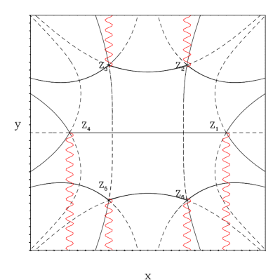
Figure 6: Stokes plot for the bound state problem $Q=E-z^{6}$.

In order to do the connections, we need the expressions $[k,l]=e^{\int_{z_{k}}^{z_{l}}i\sqrt{Q(z)}dz}$. Note that the sheet of $i\sqrt{Q(z)}$ is defined by the cut locations, with the initial sheet determined by the fact that $(z_{1},z)$ is subdominant for $x\rightarrow+\infty$ , meaning that $i\sqrt{Q}(z)=-real$ in this domain. Carrying out the integrals then gives

$$[1,2]=e^{\sqrt{3}W/4}e^{iW/4},\hskip 14.22636pt[3,2]=e^{-iW/2},\hskip 14.22636pt[3,4]=e^{-\sqrt{3}W/4}e^{iW/4},$$ (32)

where $W=E^{2/3}\int_{-1}^{1}\sqrt{1-u^{6}}du$, and $\int_{-1}^{1}\sqrt{1-u^{6}}du=1.821488$.

Begin with a subdominant solution $\psi(z)=(Z_{1},z)_{s}$ at large positive $x$ and continue through the upper half plane above all singularities to large negative $x$. Choosing the solution to be real for $x\rightarrow\infty$ and using the symmetry of the potential, but also noting that with the choice of cuts we have $Q^{1/4}=e^{i\pi/2}$ for large positive $x$ and $Q^{1/4}=e^{-i\pi/2}$ for large negative $x$ we find

$$(-1)^{n}i=1+S^{2}[1+cos(W)+isin(W)+2e^{-\sqrt{3}W/2}cos(W/2)].$$ (33)

Also we find a condition for the vanishing of the dominant solution

$$1+e^{\sqrt{3}W/2}cos(W/2)+S^{2}[e^{\sqrt{3}W/2}+2cos(W/2)+e^{-\sqrt{3}W/2}]cos(W/2)=0,$$ (34)

giving $S^{2}=-1+O(e^{-\sqrt{3}W})$.

For large turning point separation $W$ is large and we have a solution given by the isolated turning point values, $S=i$ and $W_{n}=(n+1/2)\pi$, the usual approximate WKB solution. A first order perturbation about the WKB value $W_{n}$ gives the solution

$$S=i,\hskip 28.45274ptcos(W)=-2e^{-\sqrt{3}W_{n}/2}cos(W_{n}/2).$$ (35)

It is interesting to note that these solutions break down at the second order in $\epsilon=e^{-\sqrt{3}W/2}$, meaning that one or more of the Stokes constants has a second order correction not given by Eq. 34. Note that Eq. 34 is real, but expanding $sin(W)$ in Eq. 33 through $sin(W)\simeq(-1)^{n}(1-cos^{2}(W)/2)$ gives an additional second order imaginary term, but there is no second order term to balance it, and we conclude that $S^{2}$ must possess an imaginary second order term, not given by Eq. 34, so this equation can be trusted only to first order.

Values of the exact energy levels, the WKB approximation, and the Phase Integral evaluation are shown in table II. For the ground state $E_{PI}$ has a 4 percent error, $E_{WKB}$ has a 30 percent error.

$${\bf Table\hskip 2.84526ptII.\hskip 5.69054ptEnergy\hskip 5.69054ptLevels\hskip 5.69054ptQ=E-z^{6}}\hskip 5.69054pt$$

$$\left(\begin{array}[]{c|c|c|c|c}\hline\cr n&E_{exact}&E_{wkb}&cos(W)&E_{PI}\\ \hline\cr 0&1.1448&0.8008&-0.36206&1.1009\\ 1&4.3332&4.1612&2.3888\times 10^{-2}&4.1929\\ 2&9.0731&8.9535&1.5727\times 10^{-3}&8.9508\\ 3&14.9195&14.8316&-1.0354\times 10^{-4}&14.8314\\ 4&21.7140&21.6224&-6.81617\times 10^{-6}&21.6224\end{array}\right)$$

VI A non hermitian hamiltonian

Non-Hermitian Hamiltonians having $PT$ symnmetry have been shown to have real spectra, following a conjecture by D. Bessis that the spectrum of the Hamiltonian $H=p^{2}+x^{2}+ix^{3}$ is real and positive. A non-Hermitian Hamiltonian problem studied by Bender and Boettcherbender is given by the function $Q(z)=E+(iz)^{N}$. The energy spectrum is positive because of symmetry under the product of parity and time reversal. As an example we take $N=3$.

The Stokes diagram is shown in Fig. 7, with three singular points located at $E^{1/3}e^{i\pi/2}$, $E^{1/3}e^{-i\pi/6}$, and $E^{1/3}e^{-i5\pi/6}$. Subdominant regions include the positive and negative real axis for $|x|\rightarrow\infty$. We carry out the continuation in the upper half complex plane in order to take account of the singular point at $Z_{2}$.

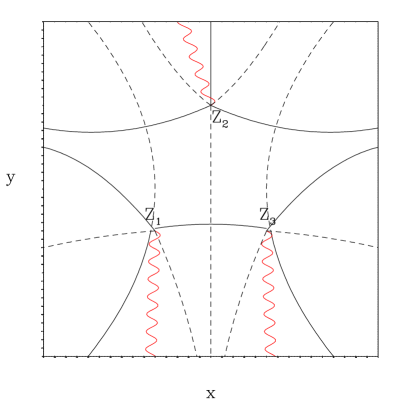
Figure 7: Stokes plot for the bound state problem, $Q=E+(iz)^{3}$.

In order to do the connections, we need the expressions $[k,l]=e^{\int_{z_{k}}^{z_{l}}i\sqrt{Q(z)}dz}$. Note that the sheet of $i\sqrt{Q(z)}$ is defined by the cut locations, with the initial sheet determined by the fact that $(z_{3},z)$ is subdominant for $x\rightarrow+\infty$ , meaning that $i\sqrt{Q}(z)=-real$ in this domain.

Carrying out the integrals then gives

$$[1,2]=e^{\sqrt{3}W/2}e^{-iW/2},\hskip 14.22636pt[1,3]=e^{-iW},\hskip 14.22636pt[2,3]=e^{-\sqrt{3}W/2}e^{-iW/2}$$ (42)

where $W=E^{5/6}cos(\pi/6)\int_{-1}^{1}\sqrt{1-u^{3}}du$, and $\int_{-1}^{1}\sqrt{1-u^{3}}du=1.68262$.

Begin for positive real $x$ with $\psi(z)=(Z_{3},z)_{s}$, and continue to large negative $x$, giving a subdominant and a dominant term, which we set to zero, giving

$$0=e^{\sqrt{3}W}(1+S^{2})+2S^{2}cos(W)+e^{-\sqrt{3}W}S^{2}$$ (43)

leaving

$$\psi(z)=-(Z_{1},z)_{s}(Se^{-\sqrt{3}W}+Se^{iW}),$$ (44)

very similar to the equations found in section IV, since the Stokes structure in the upper half plane is the same. In this case the differential equation is not real, but choosing symmetric integration paths from $x=0$ asymptotically along the Stokes lines to the right and to the left, and using the symmetry of $Q(z)$ we again conclude that the phases of the solutions for large positive $x$ and large negative $x$ are equal within a sign.

The cut locations give the fact that whereas $Q^{1/4}=e^{i\pi/4}$ for large positive $x$, $Q^{1/4}=e^{i3\pi/4}$ for large negative $x$, so in fact choosing the eigenfunction to be real for $x\rightarrow+\infty$ and requiring that it be real for large negative $x$ gives from Eq. 44 $cos(W)+e^{-\sqrt{3}W}=0$. Again in this case the asymptotic value of the Stokes constant is given by $S=i+O(\epsilon^{2})$ with $\epsilon=e^{-\sqrt{3}W}$.

The first few energy levels for $N=3$, with WKB and numerical values given by Bender, and values from this Phase Integral analysis are given in Table III. The WKB ground state energy has an error of 6 percent, and the Phase Integral value an error of 0.6 percent.

$${\bf Table\hskip 2.84526ptIII.\hskip 5.69054ptEnergy\hskip 5.69054ptLevels\hskip 5.69054ptQ=E-iz^{3}}$$

$$\left(\begin{array}[]{c|c|c|c|c}\hline\cr n&E_{exact}&E_{wkb}&cos(W)&E_{PI}\\ \hline\cr 0&1.1562&1.09427&-6.5834\times 10^{-2}&1.1496\\ 1&4.1092&4.08949&-2.8533\times 10^{-4}&4.0892\\ 2&7.5621&7.54898&-1.2366\times 10^{-6}&7.54898\\ 3&11.3143&11.3043&-5.3598\times 10^{-9}&11.3043\\ 4&15.2916&15.2832&-2.3228\times 10^{-11}&15.2832\end{array}\right)$$ (51)

VII Potentials

The four potentials for the bound state cases are plotted in Fig. 8. The harmonic oscillator potential (a) $V(x)=z^{2}-E$ and the two anharmonic oscillator potentials (c) $V(x)=z^{4}-E$ and (d) $V(x)=z^{6}-E$ are real on the real axis, $z=x$. The potential associated with $Q=E+(iz)^{3}$ (b) is real giving subdominant solutions along the lines $y=-|x|/\sqrt{3}$, with $V(x)=|x|^{3}(\sqrt{3}-1/3)-E$. The energies used in the plot are the ground state values. It is seen that the degree of distortion from the harmonic oscillator potential shape is inceasingly larger for the $(iz)^{3}$ and the $z^{4}$ and $z^{6}$ cases, associated with the larger number of singularities in $Q(z)$ in addition to the two turning point singularities. We see that the error in the WKB energy levels increases with the deviation from the harmonic oscillator potential shape, along with a corresponding improvement of the Phase Integral evaluation over the WKB value.

Figure 8: Potentials for the four bound state cases discussed, the harmonic oscillator associated with the Weber equation, $V=x^{2}-E$, (a), the non-Hermitian potential $Q=E+(iz)^{3}$ (b), and the Hermitian anharmonic oscillators $V=x^{4}-E$ (c), and $V=x^{6}-E$ (d). The exact ground state energies were used for each plot.

VIII Conclusion

A proper use of Phase Integral methods can improve the eigenvalue determination for bound states significantly compared to a simple WKB evaluation. This improvement increases along with the increasing deviation of the potential shape from that of a harmonic oscillator. For all potentials possessing zeros or singularities in the complex plane in addition to the principal turning points, a small parameter is defined by $exp{\int(i\sqrt{Q})dz}$, with the integration taken from them to the principle turning points, allowing a perturbation expansion. No such parameter exists for the Weber equation or the Budden problem. However in these cases the Stokes constants can be calculated analytically. It is remarkable that the asymptotic value of the Stokes constant in each case is $S=i$, the value for an isolated first order zero, and that in the cases examined in perturbation theory the corrections to $S$ are second order or higher in the small parameter given by the separation of the singular points. We have had to make the simplifying assumption that the Stokes constants are all equal, undoubtedly not true to higher order. The two complex equations resulting from the vanishing of the dominant solution and the symmetry or anti-symmetry of the subdominant solution do not allow proceeding to higher order, additional information is needed. It is an open question whether such relations exist, and whether the resulting equations lead to a convergent series giving the exact bound state energy. Of course the bound state energies do not form an open set, so $S$ is not determined as an analytic function of $E$, only the values at the bound eigenstates are fixed. However, we conjecture that it is a common feature that all Stokes constants associated with lines emerging from a simple zero approach $i$ for large separation between singularities.

It has not escaped the authors’ attention that with present day computing the numerically correct eigenvalues are easily obtained, so this result is only of theoretical interest.

Acknowledgement This work was partially supported by the U.S. Department of Energy Grant DE-AC02-09CH11466. The author acknowledges useful exchanges with Cheng Tang and constant encouragement from his grandson Enrico.

References

- (1) G. Wentzel, Zeit. f. Phys. 38, 518 (1926), H. A. Kramers, Zeit. f. Phys. 39, 828 (1926), L. Brillion, C. R. Acad. Sci. Paris 183, 24 (1926), H. Jeffries, Philos. Mag. [7] 33, 451 (1942)
- (2) J. Heading. An Introduction to Phase Integral Methods Wiley, NY (1962)
- (3) R. B. White, Asymptotic Analysis of Differential Equations, Imperial College Press, 2010
- (4) R. B. White, J. Comput. Phys. [31] 409 (1979)
- (5) L. Dunham, J. Phys. Rev. X. 41. 713-720. 10.1103/PhysRev.41.713 (1932).
- (6) R.B. Dingle Asymmpotic Expansions: Their Derivation and Interpretation Academic Press, London and New York (1973)
- (7) M.V. Berry and C.J. Howlse, Proc.Roy.Soc.Lond.,A430,653 (1990)
- (8) M.V. Berry, Asymmpotics, Superasymptotics, Hyperasymptotics, in Asymptotics Beyond All Orders, H. Segur et al (eds.) Plenum Press NY (1991)
- (9) M.N. Sergeenko, Physical Review A. [53] 3798 (1996)
- (10) E. Delabaere, H. Dillinger, and F. Pham, J. Math. Phys. [38] 6126 (1997)
- (11) M.N. Sergeenko, ArXiv:quant-ph/0206179v1 (2002)
- (12) A. Mirnov and A. Morozov, Journal of High Energy Physics 2010:40 (2010)
- (13) A.K. Kashani-Poor, ArXiv:1604.01690v3 (2016)
- (14) J.M. Campbell, J. Comput. Phys. 10, 308 (1972)
- (15) C. M. Bender, K. Olausson, P.S. Wang, Phys. Rev. D 16, 1740 (1977)
- (16) N. Froman, Ark. Fys. 32, 541 (1966)
- (17) M.S. Child Semiclassical Mechanics with Molecular Applications, second edition, Oxford University Press (2014)
- (18) C. M. Bender and S. Boettcher, Phys Rev Lett 80, 5243 (1998)