Deriving robust noncontextuality inequalities from algebraic proofs of the Kochen-Specker theorem: the Peres-Mermin square

Abstract

When a measurement is compatible with each of two other measurements that are incompatible with one another, these define distinct contexts for the given measurement. The Kochen-Specker theorem rules out models of quantum theory that satisfy a particular assumption of context-independence: that sharp measurements are assigned outcomes both deterministically and independently of their context. This notion of noncontextuality is not suited to a direct experimental test because realistic measurements always have some degree of unsharpness due to noise. However, a generalized notion of noncontextuality has been proposed that is applicable to any experimental procedure, including unsharp measurements, but also preparations as well, and for which a quantum no-go result still holds. According to this notion, the model need only specify a probability distribution over the outcomes of a measurement in a context-independent way, rather than specifying a particular outcome. It also implies novel constraints of context-independence for the representation of preparations. In this article, we describe a general technique for translating proofs of the Kochen-Specker theorem into inequality constraints on realistic experimental statistics, the violation of which witnesses the impossibility of a noncontextual model. We focus on algebraic state-independent proofs, using the Peres-Mermin square as our illustrative example. Our technique yields the necessary and sufficient conditions for a particular set of correlations (between the preparations and the measurements) to admit a noncontextual model. The inequalities thus derived are demonstrably robust to noise. We specify how experimental data must be processed in order to achieve a test of these inequalities. We also provide a criticism of prior proposals for experimental tests of noncontextuality based on the Peres-Mermin square.

I Introduction

Ontological models of quantum theory are an attempt to explain the statistical predictions of quantum theory. They take every system to be associated with a space of possible physical states, termed ontic states, every quantum state to be represented by a statistical distribution over these ontic states, and every measurement to be represented by a conditional probability distribution for the outcome given the ontic state Harrigan and Spekkens (2010). Hidden variable models are examples of ontological models, but so is the physicist’s orthodox conception of quantum theory, wherein the ontic states are simply the pure quantum states, not supplemented by any additional variables.

The principle of noncontextuality is an assumption about ontological models that seeks to capture a notion of classicality. It started its life as an assumption about outcome-deterministic ontological models of quantum theory, that is, ontological models wherein the outcome of every measurement was fixed deterministically by the ontic state (in contrast to the orthodox conception). This assumption was famously demonstrated to be in contradiction with the predictions of quantum theory by Kochen and Specker Kochen and Specker (1967) and Bell Mann and Crease (1988). The Kochen-Specker theorem is one of the strongest constraints on the intepretation of quantum theory. Furthermore, failing to admit of a noncontextual model appears to be a resource. For instance, in the context of the state injection model for quantum computation Bravyi and Kitaev (2005); Knill (2005), the failure of noncontextuality has been shown in some cases to be necessary for achieving universal quantum computation Howard et al. (2014); Bermejo-Vega et al. (2016).

In Ref. Spekkens (2005), a generalized notion of noncontextuality was proposed. For measurements, it constitutes a relaxation of what was assumed by Kochen-Specker and by Bell. Specifically, it allows the assignment of measurement outcomes by ontic states to be indeterministic. In this way, it redefined the notion of noncontextuality for measurements in a way that excised the notion of determinism. This is desirable from a foundational perspective as it allows one to separate the issue of noncontextuality from that of determinism (recall that Bell’s notion of local causality does not presume that the outcomes of measurements are fixed deterministically). Additionally, it can be shown that the assumption of outcome determinism is unwarranted for any unsharp measurement (i.e., a measurement for which one cannot find a basis of preparations relative to which it is perfectly predictable), and every measurement appearing in a real experiment is of this sort Spekkens (2014). As such, this generalization is important if one hopes to turn the proven theoretical advantages for computation into practical advantages, because in practice, sharpness is an idealization that is never strictly satisfied.

Although the revised notion of noncontextuality yields a weaker constraint on the representation of measurements in the ontological model than did the traditional notion, it naturally applies not only to measurements but to preparations as well, and thereby implies novel constraints on how quantum states can be represented by distributions over ontic states in the model. It was argued in Ref. Spekkens (2005) that whatever motivations can be given for assuming noncontextuality for one type of procedure, such as a measurement, this same motivation can be given for assuming it of any other type of procedure, such as a preparation. Consequently, the only natural assumption to consider in this approach is that the revised notion of noncontextuality applies to all procedures. This assumption is termed universal noncontextuality or simply noncontextuality. We will henceforth refer to the traditional notion of noncontextuality as KS-noncontextuality (for Kochen-Specker) to avoid any confusion.

In Ref. Spekkens (2005), it was shown that quantum theory does not admit of a universally noncontextual ontological model. It was also demonstrated that if one replaces the assumption of KS-noncontextuality for measurements with the assumption of universal noncontextuality for all procedures, the relaxation of the constraints on the representation of measurements is compensated by the strengthening of the constraints on the representation of preparations in such a way that any proof that quantum theory fails to admit of a KS-noncontextual model can be translated into a proof that it fails to admit of a universally noncontextual model.

Much of the research on noncontextuality to date has centered on the question of whether quantum theory admits of a noncontextual model. A more general question, which has been the impetus for much recent work, is whether one can devise a direct experimental test of the assumption of a noncontextual ontological model, one that is independent of the validity of quantum theory. Just as a Bell inequality is a constraint on experimental statistics that follows directly from the assumption of a locally causal ontological model, without any reference to the quantum formalism, what one wants of a test of noncontextuality is a constraint on experimental statistics that follows directly from the assumption of a noncontextual ontological model, without any reference to the quantum formalism. Such constraints will here be termed noncontextuality inequalities. If experimental statistics are found to violate these inequalities, then one can conclude that not just quantum theory but any operational theory that can do justice to the experimental statistics—and therefore nature itself—must fail to admit of such a model, thereby constraining the form of all future physical theories.

The generalized notion of noncontextuality proposed in Ref. Spekkens (2005) was defined in such a way as to be applicable to any operational theory, not just quantum theory, such that if an experiment yields data supporting an operational theory distinct from quantum theory, the question of whether it admits of a noncontextual model is still meaningful. The definition asserts that an ontological model of an operational theory is noncontextual if two experimental procedures that are statistically indistinguishable at the operational level are statistically indistinguishable at the ontological level. They key point is that the notion of statistical indistinguishability at the operational level can be assessed in any operational theory.

It has been shown that violations of noncontextuality inequalities defined in terms of this notion can imply advantages for information processing which are independent of the validity of quantum theory. For example, they imply an advantage for the cryptographic task of parity-oblivious random access codes Spekkens et al. (2009); Chailloux et al. (2016); Ambainis et al. (2016). Such inequalities also hold promise for making the results on quantum computational advantages discussed above robust to noise and for expressing the origin of the advantage in a manner that is independent of the validity of quantum theory.

Several recent works have considered the question of how to derive noncontextuality inequalities and how to subject them to experiment test Mazurek et al. (2016); Kunjwal and Spekkens (2015); Pusey (2015). The present work is concerned with a special case of this problem, namely, how to derive noncontextuality inequalities starting from any given proof of the Kochen-Specker theorem, that is, from a proof of the failure of KS-noncontextuality in quantum theory. As noted above, Ref. Spekkens (2005) showed how, in general, to convert a proof of the failure of KS-noncontextuality in quantum theory into a proof of the failure of universal noncontextuality in quantum theory, so the outstanding problem is how to convert a proof of the failure of universal noncontextuality in quantum theory into an operational noncontextuality inequality.

Note that any test of noncontextuality that is devised from a particular no-go theorem requires an experimentalist to target a particular set of preparations and a particular set of measurements, each with specified relations holding among their members (we will say more about the nature of these relations in due course). A more general version of the problem, however, is to figure out how to infer from any experimental data—that is, from an experiment that was not designed to target particular preparations or measurements or any particular relations among them—whether or not it admits of a noncontextual model. Because a test of noncontextuality is a test of classicality, having the capability to test the assumption of noncontextuality on any experimental data is clearly of greater utility than merely knowing how to implement a dedicated experiment for testing the hypothesis of noncontextuality. Pusey Pusey (2015) identified the conditions that are both necessary and sufficient for the existence of a noncontextual model for experimental data derived from the simplest experimental scenario in which such conditions are expected to be nontrivial. Unfortunately, this simplest scenario does not arise within operational quantum theory. Extending Pusey’s analysis to more general scenarios is an important open problem.

Nonetheless, there are also advantages to building sets of noncontextuality inequalities from specific proofs of the Kochen-Specker theorem, because such proofs have nontrivial structural properties. Different proofs—and there is now a great diversity of these—capture what is surprising about the failure of noncontextuality in different ways, and these intuitions are likely to be helpful in identifying the applications thereof.

We here focus on deriving noncontextuality inequalities from state-independent proofs of the Kochen-Specker theorem.

Ref. Kunjwal and Spekkens (2015) has already demonstrated how one can derive one such inequality from any state-independent geometric proof of the Kochen-Specker theorem, that is, any proof expressed in terms of an uncolourable set of rays. Here, we extend this work in two important ways: (1) we provide a technique for finding all of the noncontextuality inequalities that apply to a certain set of correlations starting from any state-independent proof of the Kochen-Specker theorem, and (2) we show how to do so for proofs that are expressed algebraically rather than geometrically. We expand on each of these points presently, in reverse order.

The distinction between geometric and algebraic proofs of the failure of KS-noncontextuality in quantum theory is not fundamental because one can convert any algebraic proof into a geometric form and vice-versa. Nonetheless, each proof style has its advantages. The first known proofs were geometric uncolorability proofs. Algebraic proofs arose later, but in many respects they have a logic that is easier to grasp. Indeed, the paradigm example of a proof of the Kochen-Specker theorem is now arguably the algebraic version of the Peres-Mermin square proof Peres (1991); Mermin (1993), which will be the example we focus on here.

Furthermore, the algebraic structure suggests generalizations of these proofs that might not be obvious from the geometric perspective Waegell and Aravind (2013, 2012). Although one could derive a noncontextuality inequality for the Peres-Mermin square by first expressing the latter as a geometric proof (as in Ref. Peres (1991)) and then applying the technique described in Ref. Kunjwal and Spekkens (2015), it is more useful to have a technique for deriving noncontextuality inequalities that is native to the algebraic approach. We here provide such a technique.

In order to turn a proof of the failure of universal noncontextuality in quantum theory into a noncontextuality inequality, one must operationalize the description of the experiment provided in the no-go theorem, purging it of any reference of the quantum formalism, and one must robustify the constraints on experimental data that are derived from noncontextuality, which means that these constraints must provide quantitative bounds that can be violated in principle even if the experimental operations are noisy. This progression was achieved in Ref. Kunjwal and Spekkens (2015), but the resulting inequality provided an upper bound on just a single operational quantity (an average, over certain preparation-measurement pairs, of the degree of correlation between them). The technique described in the present article goes much further towards providing a means of deriving all of the noncontextuality inequalities that hold for a given set of preparations and measurements. Although we focus on a subset of the correlations between preparations and measurements that arise in the construction, for this restricted set of experimental data, satisfaction of the inequalities that we derive is both necessary and sufficient for the existence of a noncontextual model.

Finally, we note a difference in the way experiments are described in this article relative to previous treatments of inequalities for universal noncontextuality Spekkens et al. (2009); Mazurek et al. (2016); Kunjwal and Spekkens (2015). We here use the notion of a source, that is, a process which samples a classical variable from a distribution, chooses which preparation procedure to implement on the system based on the value sampled and outputs both the system and the variable. This choice ensures that our derived noncontexuality inequalities are easier to compare with Bell inequalities.

The remainder of the paper is structured as follows.

In Section II, we provide an overview of operational theories (II.II.1) and ontological models (II.II.2). In particular, we discuss the concepts of operational equivalence and of compatibility (applied to measurements and sources) and illustrate the concepts with quantum examples. We provide formal definitions of measurement noncontextuality and preparation noncontextuality, in particular, a characterization of these assumptions in terms of expectation values for the outcomes of measurements and sources given the ontic state.

In Section III, we review the well-known proof of the failure of KS-noncontextuality in quantum theory based on the Peres-Mermin square (III.III.1), and we show how to translate this no-go theorem into one that demonstrates the failure of universal noncontextuality in quantum theory (III.III.2).

Section IV is the heart of the article, describing our technique for turning quantum no-go theorems into operational noncontextuality inequalities. In the first subsection (IV.IV.1), we operationalize the description of the quantum measurements and sources that appear in the Peres-Mermin-inspired proof of the failure of universal noncontextuality, thereby obtaining a notion of a Peres-Mermin experimental scenario that is purged of any reference to quantum theory. This provides a template for how to achieve this operationalization for any such construction. The following five subsections (IV.IV.2-IV.IV.6) describe how to derive noncontextuality inequalities from such an operational construction, using Peres-Mermin as the illustrative example. We also show how the ideal quantum realization of the measurements and sources in the Peres-Mermin scenario violate these inequalities (IV.IV.6.IV.6.1), and we demonstrate the robustness of these inequalities to noise (IV.IV.6.IV.6.2), by showing how they can be violated by partially depolarized versions of the ideal quantum realizations of the measurements and sources.

In Section V, we clarify what must be done experimentally in order to test the noncontextuality inequalities we have derived, and in Section VI we provide our concluding remarks.

Appendix A discusses the problem of computationally converting between the vertex and halfspace representations of a polytope., Appendix B discusses the symmetries of our noncontextuality inequalities under deterministic processings of the experimental procedures, and Appendix C demonstrates that a certain class of inequalities on experimental statistics are trivial. Finally, Appendix D reviews a previous proposal for how to implement an experimental test of noncontextuality based on the Peres-Mermin square, and argues against its adequacy.

II Preliminaries

II.1 Operational concepts

II.1.1 Operational theories

The primitive elements of an operational theory are preparations and measurements, each specified as lists of instructions to be performed in the laboratory.

A source is a device that implements one of a set of preparation procedures on a system, sampled from some probability distribution, and has a classical outcome that heralds which preparation has in fact been implemented. (The use of the term “source” to refer to such a device is conventional in both classical and quantum Shannon theory, where it is the standard way of modelling the input to a communication channel Preskill (2000).) We will denote a source by $\operatorname{S}$ and the variable describing its classical outcome by $s$.

A measurement, denoted $\operatorname{M}$, accepts as input a system and returns a classical outcome, denoted by the variable $m$.

An operational theory provides an algorithm for computing the probability distribution for the outcome of any measurement acting on any preparation, and consequently it allows the computation of the joint probability distribution over the outcome of any measurement $\operatorname{M}$ and the outcome of any source $S$, $\operatorname{pr}\{m,s|\operatorname{M},\operatorname{S}\}$. We refer to this as simply the joint distribution on the measurement-source pair $(M,S)$.

II.1.2 Operational equivalence

Consider two measurement procedures, $\operatorname{M}_{1}$ and $\operatorname{M}_{2}$, whose outcomes are random variables, denoted $m_{1}$ and $m_{2}$ respectively. $\operatorname{M}_{1}$ and $\operatorname{M}_{2}$ are said to be operationally equivalent if they define the same joint distribution for all possible sources:

$$\forall S:\operatorname{pr}\{m_{1},s|\operatorname{M}_{1},\operatorname{S}\}=\operatorname{pr}\{m_{2},s|\operatorname{M}_{2},\operatorname{S}\}.$$ (1)

Letting $\mathcal{M}$ denote an operational equivalence class of measurements, we can express the operational equivalence of two measurements $\operatorname{M}_{1}$ and $\operatorname{M}_{2}$ by specifying that they belong to the same class,

$$\operatorname{M}_{1},\operatorname{M}_{2}\in\mathcal{M}.$$ (2)

Similarly, two sources, $\operatorname{S}_{1}$ and $\operatorname{S}_{2}$, whose outcomes are random variables $s_{1}$ and $s_{2}$ respectively, are said to be operationally equivalent if they define the same joint distibution for all possible measurements:

$$\forall\operatorname{M}:\operatorname{pr}\{m,s_{1}|\operatorname{M},\operatorname{S}_{1}\}=\operatorname{pr}\{m,s_{2}|\operatorname{M},\operatorname{S}_{2}\}.$$ (3)

Letting $\mathcal{S}$ denote an operational equivalence class of sources, we can express the operational equivalence of two sources, $\operatorname{S}_{1}$ and $\operatorname{S}_{2}$, by stipulating that they are in the same class,

$$\operatorname{S}_{1},\operatorname{S}_{2}\in\mathcal{S}.$$ (4)

Because the joint distribution $\operatorname{pr}\{s,m|\operatorname{M},\operatorname{S}\}$ is computable from the operational theory, so too is the correlation between the outcome $s$ of the source $\operatorname{S}$ and the outcome $m$ of the measurement $\operatorname{M}$,

$$\langle sm\rangle_{\operatorname{M},\operatorname{S}}=\sum_{s,m}sm\operatorname{pr}\{s,m|\operatorname{M},\operatorname{S}\}~{}.$$ (5)

Such correlations will be the quantities appearing in our noncontextuality inequalities.

II.1.3 Compatibility

In this section, we briefly review the notion of compatibility. The interested reader is pointed to Liang et al. (2011) for a detailed overview.

Informally, two or more devices are said to be compatible if their output can be obtained by classical post-processing of the output of a single device. More precisely, one can define the notion of compatibility in terms of a notion of simulatability.

Consider two measurements, $\operatorname{M}$ and $\operatorname{M}^{\prime}$, which accept an input system and output random variables $m$ and $m^{\prime}$ respectively. We say that $\operatorname{M}$ can simulate $\operatorname{M}^{\prime}$ if there exists a conditional distribution $\operatorname{pr}\{m^{\prime}|m\}$ such that

$$\forall\operatorname{S}:\operatorname{pr}\{m^{\prime}\!,s|\operatorname{M}^{\prime}\!,\operatorname{S}\}=\sum_{m}\operatorname{pr}\{m^{\prime}|m\}\operatorname{pr}\{m,s|\operatorname{M},\operatorname{S}\}\!.$$ (6)

Two measurements $\operatorname{M}_{1}$ and $\operatorname{M}_{2}$ are said to be compatible if both of them can be simulated by some third measurement $\operatorname{M}$, that is, if there exists $\operatorname{pr}\{m_{1}|m\}$ and $\operatorname{pr}\{m_{2}|m\}$ such that

$$\begin{split}\forall\operatorname{S}:\operatorname{pr}\{m_{1},s|\operatorname{M}_{1},\operatorname{S}\}\!=\!\sum_{m}\operatorname{pr}\{m_{1}|m\}\!\operatorname{pr}\{m,s|\operatorname{M},\operatorname{S}\},\\ \forall\operatorname{S}:\operatorname{pr}\{m_{2},s|\operatorname{M}_{2},\operatorname{S}\}\!=\!\sum_{m}\operatorname{pr}\{m_{2}|m\}\!\operatorname{pr}\{m,s|\operatorname{M},\operatorname{S}\}.\end{split}$$ (7)

Similar definitions hold for sources. We say that a source $\operatorname{S}$ with classical outcome $s$ simulates source $\operatorname{S}^{\prime}$ with classical outcome $s^{\prime}$ if there exists a conditional distribution $\operatorname{pr}\{s^{\prime}|s\}$ such that

$$\forall\operatorname{M}:\operatorname{pr}\{m,s^{\prime}|\operatorname{M},\operatorname{S}^{\prime}\}\!=\!\sum_{s}\operatorname{pr}\{s^{\prime}|s\}\!\operatorname{pr}\{m,s|\operatorname{M},\operatorname{S}\}.$$ (8)

When it comes to defining a notion of compatibility of sources, there is a nuance relative to the case of measurements. The definition we adopt will apply only to those pairs of sources, $\operatorname{S}_{1}$ and $\operatorname{S}_{2}$, that are operationally equivalent when one marginalizes over their outcomes, that is, it presumes that $\operatorname{S}_{1}$ and $\operatorname{S}_{2}$ are such that

$$\forall\operatorname{M}:\sum_{s_{1}}\operatorname{pr}\{m,s_{1}|\operatorname{M},\operatorname{S}_{1}\}=\sum_{s_{2}}\operatorname{pr}\{m,s_{2}|\operatorname{M},\operatorname{S}_{2}\}.$$ (9)

Every set of sources we consider in this article will have this property. Two such sources, $\operatorname{S}_{1}$ and $\operatorname{S}_{2}$, are said to be compatible if there exists a third source $\operatorname{S}$ that simulates them both, that is, if there exists $\operatorname{pr}\{s_{1}|s\}$ and $\operatorname{pr}\{s_{2}|s\}$ such that

$$\begin{split}\forall\operatorname{M}:\operatorname{pr}\{m,s_{1}|\operatorname{M},\operatorname{S}_{1}\}\!=\!\sum_{s}\operatorname{pr}\{s_{1}|s\}\!\operatorname{pr}\{m,s|\operatorname{M},\operatorname{S}\},\\ \forall\operatorname{M}:\operatorname{pr}\{m,s_{2}|\operatorname{M},\operatorname{S}_{2}\}\!=\!\sum_{s}\operatorname{pr}\{s_{2}|s\}\!\operatorname{pr}\{m,s|\operatorname{M},\operatorname{S}\}.\end{split}$$ (10)

It is instructive to consider what these notions of compatibility correspond to in quantum theory.

Recall that every measurement in quantum theory is represented by a positive operator-valued measure (POVM) whose elements are labelled by the outcome $m$, that is, by $\{E_{m}\}_{m}$ where $\forall m:E_{m}\geq 0$ and $\sum_{m}E_{m}=\mathbb{1}$.

Every source in quantum theory is represented by an ensemble of subnormalized quantum states $\{p_{s}\rho_{s}\}_{s}$ where $\forall s:\rho_{s}\geq 0,{\rm Tr}(\rho_{s})=1$ and $p_{s}$ is a probability distribution over $s$. In other words, the ensemble $\{p_{s}\rho_{s}\}_{s}$ defines the source that samples $s$ from the probability distribution $p_{s}$, then prepares the quantum system in the normalized state $\rho_{s}$ and outputs $s$ as its outcome.

If a measurement $\operatorname{M}$ is represented by the POVM $\{E_{m}\}_{m}$ and a source $S$ is represented by the ensemble $\{p_{s}\rho_{s}\}_{s}$, then the probability of the source generating outcome $s$ and the measurement generating outcome $m$ is given by the Born rule as $\operatorname{pr}\{m,s|\operatorname{M},\operatorname{S}\}={\rm Tr}(E_{m}p_{s}\rho_{s})$.

Substituting this Born rule expression into Eq. (7), we infer that if two measurements, associated to POVMs $\{E_{m_{1}}\}_{m_{1}}$ and $\{E_{m_{2}}\}_{m_{2}}$, are compatible, then there exists a third POVM $\{E_{m}\}_{m}$ and conditional distributions $\operatorname{pr}\{m_{1}|m\}$ and $\operatorname{pr}\{m_{2}|m\}$ such that

$$\begin{split}E_{m_{1}}=\sum_{m}\operatorname{pr}\{m_{1}|m\}E_{m},\\ E_{m_{2}}=\sum_{m}\operatorname{pr}\{m_{2}|m\}E_{m}.\end{split}$$

For two quantum sources, associated to ensembles $\{p_{s_{1}}\rho_{s_{1}}\}_{s_{1}}$ and $\{p_{s_{2}}\rho_{s_{2}}\}_{s_{2}}$, the property that ensures the applicability of our definition of compatibility, Eq. (9), is that the two ensembles define the same average state, $\sum_{s_{1}}p_{s_{1}}\rho_{s_{1}}=\sum_{s_{2}}p_{s_{2}}\rho_{s_{2}}$. Substituting the Born rule expression into Eq. (8), we infer that if the two quantum sources are compatible, then there exists a third ensemble ${\{p_{s}\rho_{s}\}_{s}}$ and conditional distributions ${\operatorname{pr}\{s_{1}|s\}}$ and ${\operatorname{pr}\{s_{2}|s\}}$ such that

$$\begin{split}p_{s_{1}}\rho_{s_{1}}=\sum_{m}\operatorname{pr}\{s_{1}|s\}p_{s}\rho_{s},\\ p_{s_{2}}\rho_{s_{2}}=\sum_{m}\operatorname{pr}\{s_{2}|s\}p_{s}\rho_{s}.\end{split}$$ (11)

Note that the notion of compatibility for quantum measurements that we have articulated above Busch et al. (1997) concerns only their retrodictive aspect and makes no reference to how the quantum state of a system evolves as a result of the measurement. In other words, it is sufficient to know which POVM is associated to the measurement, while the instrument that is associated to it, i.e., the set of update maps for each outcome, is irrelevant (indeed, it is not even required that there be an update map—the quantum system could be destroyed in the measurement process). This contrasts with the notion of compatibility that is the focus of many other works seeking to devise experimental tests of noncontextuality Kirchmair et al. (2009), where two measurements on a system are deemed compatible if implementing them in one temporal order gives the same statistics as implementing them in the opposite temporal order. The joint-simulatability notion of compatibility articulated above pertains not just to sharp measurements (represented by projector-valued measures) but to all unsharp measurements as well (represented by positive operator-valued measures). In particular, it allows nontrivial compatibility relations among unsharp measurements that are associated to POVMs wherein the different elements of the POVM do not commute with one another, whereas such POVMs need not even compatible with themselves according to the temporal-reordering notion of compatibility. The wide scope of applicability of the joint-simulatability notion of compatibility makes it particulary well-equipped to contend with experimental noise and imperfections in tests of noncontextuality.

A given POVM defines an operational equivalence class of measurements insofar as it can be implemented in many different ways. This is because any given POVM is generally compatible with many other POVMs which are not compatible with one another, and for each such compatible set of POVMs, there is a different experimental procedure, and hence a different concrete realization of the given POVM. The compatible set of which the POVM is considered a part is therefore an example of a measurement context. Note that if one particularizes the definition of compatibility to projector-valued measures, then the condition for compatibility becomes commutativity of the associated observables, and we recover the standard notion of a measurement context of an observable as the commuting set of observables of which it is considered a part. The important point, however, is that in addition to recovering the standard notion of measurement context for sharp (i.e., projective) measurements, one has a notion of measurement context also for unsharp measurements.

In a similar fashion, a given ensemble of quantum states defines an operational equivalence class of sources because it too can be implemented in many different ways, depending on which compatible set of ensembles it is considered to be a member of. The compatible set of ensembles of which it is a member constitutes the source context. It will later be useful to distinguish between sharp and unsharp quantum sources, where sharp sources are those consisting entirely of states that are normalizd projectors. Clearly, the notion of compatibility of sources that we have introduced applies equally well to sharp and unsharp quantum sources, just as the notion for measurements applies to the sharp and unsharp cases alike.

II.2 Ontological concepts

II.2.1 Ontological models

As proposed in Ref. Spekkens (2005), generalized noncontextuality is a constraint on an ontological model of an operational theory. An ontological model is an attempt to reproduce the predictions of the operational theory by imagining that the correlations between the outcome of the source and that of the measurement are explained by the physical system that acts as a causal mediary between them. All of the physical attributes of the system at any given point in time is termed the ontic state of the system at that time. We shall denote this by $\lambda$, and the space of all possible ontic states of the system will be denoted by $\Lambda$.

Consider the most general way of representing a measurement procedure $\operatorname{M}$ in an ontological model. The output $m$ might not be completely determined by the ontic state $\lambda$ of the system. Instead, specifying $\operatorname{M}$ might only specify the conditional probability of obtaining output $m$ if the system is in the ontic state $\lambda$. This could arise because of objective indeterminism or because the outcome of the measurement depends not only on the input system but also on degrees of freedom of the measurement apparatus. We denote this conditional probability by $\xi\left(m|\lambda,\operatorname{M}\right)$ and refer to it as the response function associated to $\operatorname{M}$.

Similarly, the most general way of representing a preparation procedure in an ontological model is to allow that the preparation does not uniquely fix the ontic state of the system, but rather that the ontic state might only be sampled probabilistically from a distribution that is specified by the preparation. This implies that the most general way of representing a source $\operatorname{S}$ in an ontological model is as a joint distribution over its outome $s$ and the ontic state $\lambda$ that it outputs, $\mu(\lambda,s|\operatorname{S})$.

The purpose of an ontological model for an operational theory is to reproduce the statistics of that theory. This occurs if the ontological model is such that for all sources $\operatorname{S}$ and measurements $\operatorname{M}$,

$$\operatorname{pr}\{m,s|\operatorname{M},\operatorname{S}\}=\sum_{\lambda\in\Lambda}\xi\left(m|\lambda,\operatorname{M}\right)\mu(\lambda,s|\operatorname{S})~{}.$$ (12)

It is useful to express the connection between the ontological model and the operational theory in terms of expectation values as well.

The expectation value of outcome $m$ of measurement $\operatorname{M}$ for the ontic state $\lambda$ is

$$\langle m\rangle_{\lambda,\operatorname{M}}\equiv\sum_{m}m\;\xi\left(m|\lambda,\operatorname{M}\right).$$ (13)

The expectation value of outcome $s$ of measurement $\operatorname{S}$ for the ontic state $\lambda$ is a retrodictive expectation value and so is a bit more subtle to express. Consider a source $\operatorname{S}$ with classical outcome $s$ that is associated with the joint distribution $\mu(\lambda,s|\operatorname{S})$. What probability ought one to assign to the outcome variable $s$ having taken a particular value if one knows that the ontic state emitted by the source was $\lambda$? The answer is given by a simple Bayesian inversion:

$$\mu(s|\lambda,\operatorname{S})=\frac{\mu(s,\lambda|\operatorname{S})}{\mu(\lambda|\operatorname{S})}$$ (14)

where

$$\mu(\lambda|\operatorname{S})\equiv\sum_{s^{\prime}}\mu(s^{\prime},\lambda|\operatorname{S}).$$ (15)

We can then use this conditional probability to define an expectation value for an outcome $s$ of a source $\operatorname{S}$ given knowledge of the ontic state $\lambda$, as:

$$\langle s\rangle_{\lambda,S}\equiv\sum_{s}s\mu(s|\lambda,\operatorname{S})~{},$$ (16)

It follows that the correlation between $m$ and $s$ can be expressed as

$$\begin{split}\langle ms\rangle_{\operatorname{M},\operatorname{S}}&=\sum_{m,s}ms\operatorname{pr}\{m,s|\operatorname{M},\operatorname{S}\}\\ &=\sum_{\lambda\in\Lambda}\langle m\rangle_{\lambda,M}\langle s\rangle_{\lambda,S}\;\mu(\lambda|\operatorname{S}),\end{split}$$ (17)

where we have used Eqs. (12, 13, 14, and 16). We will use the latter expression when deriving our quantum no-go theorems and noncontextuality inequalities.

II.2.2 Measurement noncontextuality

The assumption of measurement noncontextuality stipulates that if two measurements $\operatorname{M}_{1}$ and $\operatorname{M}_{2}$ are operationally equivalent, then the response functions associated to these measurements in the ontological model are equal. Equivalently, we can express measurement noncontextuality as the assumption that the response function associated to a measurement depends only on its operational equivalence class and not on the measurement context (which explains the appropriateness of the term “noncontextual”). Denoting the operational equivalence class of $\operatorname{M}_{1}$ and $\operatorname{M}_{2}$ by $\mathcal{M}$ (with outcome denoted by $m$), and denoting the response function for $\operatorname{M}_{1}$ and $\operatorname{M}_{2}$ and $\mathcal{M}$ by $\xi\left(m_{1}|\lambda,\operatorname{M}_{1}\right)$, $\xi\left(m_{2}|\lambda,\operatorname{M}_{2}\right)$ and $\xi\left(m|\lambda,\operatorname{M}\right)$ respectively, the assumption of measurement noncontextuality can be formalized as follows:

$$\begin{split}&\text{If }\operatorname{M}_{1},\operatorname{M}_{2}\in\mathcal{M}\text{, then}\;\;\forall\;{\lambda\in\Lambda}:\\ &\quad\xi\left(m_{1}|\lambda,\operatorname{M}_{1}\right)=\xi\left(m_{2}|\lambda,\operatorname{M}_{2}\right)\equiv\xi\left(\mathcal{m}|\lambda,\mathcal{M}\right).\end{split}$$ (18)

We can also express measurement noncontextuality in terms of expectation values, using Eq. (13), as

$$\begin{split}&\text{If }\operatorname{M}_{1},\operatorname{M}_{2}\in\mathcal{M}\text{, then}\;\;\forall\;{\lambda\in\Lambda}:\\ &\qquad\langle m_{1}\rangle_{\lambda,\operatorname{M}_{1}}=\langle m_{2}\rangle_{\lambda,\operatorname{M}_{2}}\equiv\langle\mathcal{m}\rangle_{\lambda,\mathcal{M}}.\end{split}$$ (19)

An ontic state $\lambda$ will be said to be make a deterministic assignment to an equivalence class of measurements $\mathcal{M}$ if

$$\xi\left(\mathcal{m}|\lambda,\mathcal{M}\right)\in\{0,1\},$$ (20)

or equivalently, if $\langle\mathcal{m}\rangle_{\lambda,\mathcal{M}}\in\textrm{Range}(\mathcal{m})$.

We pause to note the how the standard notion of measurement context that appears in proofs of the Kochen-Specker theorem is understood in our framework. Consider a measurement associated to an observable $\operatorname{O}$. If $\operatorname{O}$ is compatible with $\operatorname{O}_{1}$ and $\operatorname{O}$ is compatible with $\operatorname{O}_{2}$, but $\operatorname{O}_{1}$ and $\operatorname{O}_{2}$ are not compatible with one another, then there are two operationally equivalent ways of implementing a measurement of $\operatorname{O}$, namely, by measuring it jointly with $\operatorname{O}_{1}$ and by measuring it jointly with $\operatorname{O}_{2}$. If $\langle m_{1}\rangle_{\lambda,\operatorname{O}(\operatorname{O}_{1})}$ denotes the expectation value for the outcome of the $\operatorname{O}$ measurement when it is measured jointly with $\operatorname{O}_{1}$ and $\langle m_{2}\rangle_{\lambda,\operatorname{O}(\operatorname{O}_{2})}$ denotes the expectation value for the outcome of the $\operatorname{O}$ measurement when it is measured jointly with $\operatorname{O}_{2}$, then measurement noncontextuality implies that $\forall\lambda\in\Lambda:\langle m_{1}\rangle_{\lambda,\operatorname{O}(\operatorname{O}_{1})}=\langle m_{2}\rangle_{\lambda,\operatorname{O}(\operatorname{O}_{2})}\equiv\langle\mathcal{m}\rangle_{\lambda,\operatorname{O}}.$ The fact that the notion of measurement noncontextuality does not include the assumption of outcome determinism translates, in the case of quantum observables, to the fact that these expectation values are not assumed, a priori, to lie in the eigenspectrum of $\operatorname{O}$.

The generalized notion of noncontextuality allows one to extend this analysis to the case of a quantum measurement that is associated to a POVM that is nonprojective. If it can be measured jointly with either one of two other POVMs which are not compatible with one another, then the assumption of measurement noncontextuality implies that the expectation value of its outcome given the ontic state $\lambda$ should be independent of which of the two other POVMs it is measured jointly with.

II.2.3 Preparation noncontextuality

The assumption of preparation noncontextuality has previously been expressed in terms of individual preparations. However, in this article we will be describing experiments in terms of sources, and so we will here express it in the language of sources.

The assumption of preparation noncontextuality stipulates that if two sources $\operatorname{S}_{1}$ and $\operatorname{S}_{2}$ are operationally equivalent, then the joint distributions over ontic states and outcomes that represent these sources in the ontological model are equal. Equivalently, the joint distribution over ontic states and outcomes representing a source depends only on the operational equivalence class of that source. Denoting the operational equivalence class of $\operatorname{S}_{1}$ and $\operatorname{S}_{2}$ by $\mathcal{S}$ (with outcome denoted by $\mathcal{s}$), and denoting the joint distribution over ontic states and outcomes for $\operatorname{S}_{1}$ and $\operatorname{S}_{2}$ and $\mathcal{S}$ by $\mu\left(s_{1},\lambda|\operatorname{S}_{1}\right)$, $\mu\left(s_{2},\lambda|\operatorname{S}_{2}\right)$, and $\mu\left(\mathcal{s},\lambda|\mathcal{S}\right)$ respectively, the assumption of preparation noncontextuality can be formalized as follows:

$$\begin{split}&\text{If }\operatorname{S}_{1},\operatorname{S}_{2}\in\mathcal{S}\text{, then}\;\;\forall\;{\lambda\in\Lambda}:\\ &\qquad\mu\left(s_{1},\lambda|\operatorname{S}_{1}\right)=\mu\left(s_{2},\lambda|\operatorname{S}_{2}\right)\equiv\mu\left(\mathcal{s},\lambda|\mathcal{S}\right).\end{split}$$ (21)

Note that an individual preparation can be understood as a special kind of source, one wherein the outcome is trivial (i.e. taking a value in a singleton set), and for such sources the definition of noncontextuality provided above reduces to the standard one for preparations articulated in Ref. Spekkens (2005).

We can also express this assumption in terms of expectation values, as we did for the case of measurements, but with a critical difference, as noted above Eq. (16): for sources, the relevant expectation values concern retrodictions rather than predictions.

If two sources, $\operatorname{S}_{1}$ and $\operatorname{S}_{2}$, are operationally equivalent then not only does preparation noncontextuality imply that the distributions $\mu\left(s_{1},\lambda|\operatorname{S}_{1}\right)$ and $\mu\left(s_{2},\lambda|\operatorname{S}_{2}\right)$ are equal (and hence the marginals $\mu\left(\lambda|\operatorname{S}_{1}\right)$ and $\mu\left(\lambda|\operatorname{S}_{2}\right)$ are equal as well), it also implies, via Eq. (14), that the conditional distributions $\mu\left(s_{1}|\lambda,\operatorname{S}_{1}\right)$ and $\mu\left(s_{2}|\lambda,\operatorname{S}_{2}\right)$ are equal as well. That is, applying Eq. (14) to Eq. (21), we find that we can express the assumption of preparation noncontextuality as

$$\begin{split}&\text{If }\operatorname{S}_{1},\operatorname{S}_{2}\in\mathcal{S}\text{, then}\;\;\forall\;{\lambda\in\Lambda}:\\ &\qquad\mu\left(s|\lambda,\operatorname{S}_{1}\right)=\mu\left(s|\lambda,\operatorname{S}_{2}\right)\equiv\mu\left(s|\lambda,\mathcal{S}\right).\end{split}$$ (22)

or, translating this into expectation values using Eq. (16), we can express it as

$$\begin{split}&\text{If }\operatorname{S}_{1},\operatorname{S}_{2}\in\mathcal{S}\text{, then}\;\;\forall\;{\lambda\in\Lambda}:\\ &\qquad\langle s_{1}\rangle_{\lambda,\operatorname{S}_{1}}=\langle s_{2}\rangle_{\lambda,\operatorname{S}_{2}}\equiv\langle\mathcal{s}\rangle_{\lambda,\mathcal{S}}.\end{split}$$ (23)

It is apparent, therefore, that the assumption of noncontextuality for sources is a kind of retrodictive analogue of the assumption of noncontextuality for measurements.

An ontic state $\lambda$ will be said to be make a deterministic assignment to an equivalence class of sources $\mathcal{S}$ if

$$\mu\left(\mathcal{s}|\lambda,\mathcal{S}\right)\in\{0,1\},$$ (24)

or equivalently, if $\langle\mathcal{s}\rangle_{\lambda,\mathcal{S}}\in\textrm{Range}(\mathcal{s})$.

We again pause to illustrate these notions by specializing to the quantum case. Consider a quantum source associated to the ensemble $\operatorname{\mathcal{E}}=\{p_{s}\rho_{s}\}$. Suppose that $\operatorname{\mathcal{E}}$ is compatible with an ensemble $\operatorname{\mathcal{E}}_{1}=\{p_{s_{1}}\rho_{s_{1}}\}$ and that it is also compatible with an ensemble $\operatorname{\mathcal{E}}_{2}=\{p_{s_{2}}\rho_{s_{2}}\}$ but that $\operatorname{\mathcal{E}}_{1}$ and $\operatorname{\mathcal{E}}_{2}$ are not compatible with one another. In this case, there are two operationally equivalent ways of implementing the source associated to $\operatorname{\mathcal{E}}$, namely, by implementing it jointly with $\operatorname{\mathcal{E}}_{1}$ and by implementing it jointly with $\operatorname{\mathcal{E}}_{2}$. If $\langle s_{1}\rangle_{\lambda,\operatorname{\mathcal{E}}(\operatorname{\mathcal{E}}_{1})}$ denotes the expectation value for the outcome of the source $\operatorname{\mathcal{E}}$ when it is implemented jointly with $\operatorname{\mathcal{E}}_{1}$ and $\langle s_{2}\rangle_{\lambda,\operatorname{\mathcal{E}}(\operatorname{\mathcal{E}}_{2})}$ denotes the expectation value for the outcome of the source $\operatorname{\mathcal{E}}$ when it is implemented jointly with $\operatorname{\mathcal{E}}_{2}$, then preparation noncontextuality implies that $\forall\lambda\in\Lambda:\langle s_{1}\rangle_{\lambda,\operatorname{\mathcal{E}}(\operatorname{\mathcal{E}}_{1})}=\langle s_{2}\rangle_{\lambda,\operatorname{\mathcal{E}}(\operatorname{\mathcal{E}}_{2})}\equiv\langle\mathcal{s}\rangle_{\lambda,\operatorname{\mathcal{E}}}.$

II.2.4 Universal noncontextuality

An operational theory will be said to admit of a universally noncontextual ontological model if it admits of an ontological model that is noncontextual for all experimental procedures, and therefore for both the preparations and the measurements Spekkens (2005).

III Quantum no-go theorems based on the Peres-Mermin square

KS-noncontextuality can be understood as the conjunction of the assumption of measurement noncontextuality defined above and the assumption that the ontic state assigns outcomes to projective measurements deterministically. It is well known that quantum theory does not admit of a KS-noncontextual model. The Peres-Mermin proof Peres (1991); Mermin (1993) is particularly intuitive and has therefore become a paradigm example.

Ref. Spekkens (2005) provided several reasons for adopting the notion of universal noncontextuality described in the previous section rather than KS-noncontextuality. First of all, the reference to projective measurements in the definition of KS-noncontextuality makes it clear that the notion of KS-noncontextuality can only be applied to quantum theory and leaves open the question of how to apply it to other operational theories or to experimental data. Furthermore, it has been argued in Refs. Spekkens (2005, 2014) that the notion of universal noncontextuality stands to the notion of KS-noncontextuality as the notion of local causality stands to that of local determinism (defined by Bell in Ref. Bell (1966)). The problem with both KS-noncontextuality and local determinism is that in the face of a contradiction, one can always salvage the spirit of noncontextuality or locality by simply abandoning determinism. Such an option is not available if one derives a contradiction from universal noncontextuality or local causality.

It was shown in Sec. VIII. of Ref. Spekkens (2005) that one can turn any no-go theorem for a KS-noncontextual model of quantum theory into a no-go theorem for a universally noncontextual model of quantum theory. In this section, we carry out this translation for the proof based on the Peres-Mermin square. This will serve to clarify the constrast between KS-noncontextuality and universal noncontextuality. However, the main purpose of this section is to provide the reader with some intuition about how the contradiction arises, so that she may better follow our technique for deriving noncontextuality inequalities from the Peres-Mermin construction.

III.1 No-go theorem for KS-noncontextuality based on the Peres-Mermin square

The Peres-Mermin magic square construction Peres (1991); Mermin (1993) consists of nine observables, each defined on two qubits and each expressible as a product of Pauli operators. Denoting the four Pauli operators by:

$$\begin{split}\mathbb{1}=\left(\begin{matrix}1&0\\ 0&1\\ \end{matrix}\right),\quad\quad&X=\left(\begin{matrix}0&1\\ 1&0\\ \end{matrix}\right),\\ Y=\left(\begin{matrix}0&i\\ -i&0\\ \end{matrix}\right),\quad\quad&Z=\left(\begin{matrix}1&0\\ 0&-1\\ \end{matrix}\right),\end{split}$$ (25)

the nine observables relevant to the construction are as follows:

$$\begin{matrix}X\otimes\mathbb{1}\;\;\;\;&\mathbb{1}\otimes X\;\;\;\;\;&X\otimes X\\ \\ \mathbb{1}\otimes Z\;\;\;\;\;&Z\otimes\mathbb{1}\;\;\;\;\;&Z\otimes Z\\ \\ X\otimes Z\;\;\;\;\;&Z\otimes X\;\;\;\;\;&Y\otimes Y\\ \end{matrix}$$ (26)

These are organized into a $3\times 3$ grid (the “square”) to visually represent their commutativity properties: the three observables on any row or column of the square commute and therefore are jointly measurable.

KS-noncontextuality implies that every observable in the square is assigned a value deterministically by the ontic state $\lambda$ and independently of whether that observable is measured together with the other observables in its row or whether it is measured together with the other observables in its column. The deterministic value assigned to observable $O$ by the ontic state $\lambda$ we denote by $\lfloor O\rfloor_{\lambda}$. Because an observable is only ever found to take values from the eigenspectrum of the associated operator, it follows that the deterministic assignments to $O$ by $\lambda$ can only take values in this set,

$$\lfloor O\rfloor_{\lambda}\in{\rm spec}(O).$$ (27)

Finally, for any set of observables that can be jointly measured, the functional relations that hold among the observables in the set must also hold among the values assigned to them by the ontic state. This follows from the fact that if a given functional relation failed to hold for the values assigned by the ontic state, then the ontological model would predict that it failed to hold for the values obtained in a joint measurement. In the Peres-Mermin square, one can show that the product of the observables along each of the rows and along each of the first two columns is $\mathbb{1}\otimes\mathbb{1}$, while the product of the observables on the last column is $-\mathbb{1}\otimes\mathbb{1}$. Therefore, the functional relations are

$$(X\otimes\mathbb{1})(\mathbb{1}\otimes X)(X\otimes X) = \hphantom{-}\,\,\mathbb{1}\otimes\mathbb{1},$$ (28a)

$$(\mathbb{1}\otimes Z)(Z\otimes\mathbb{1})(Z\otimes Z) = \hphantom{-}\,\,\mathbb{1}\otimes\mathbb{1},$$ (28b)

$$(X\otimes Z)(Z\otimes X)(Y\otimes Y) = \hphantom{-}\,\,\mathbb{1}\otimes\mathbb{1},$$ (28c)

$$(X\otimes\mathbb{1})(\mathbb{1}\otimes Z)(X\otimes Z) = \hphantom{-}\,\,\mathbb{1}\otimes\mathbb{1},$$ (28d)

$$(\mathbb{1}\otimes X)(Z\otimes\mathbb{1})(Z\otimes X) = \hphantom{-}\,\,\mathbb{1}\otimes\mathbb{1},$$ (28e)

$$(X\otimes X)(Z\otimes Z)(Y\otimes Y) = -\mathbb{1}\otimes\mathbb{1}.$$ (28f)

Together with the fact, inferred from Eq. (27), that

$$\begin{split}\lfloor\mathbb{1}\otimes\mathbb{1}\rfloor_{\lambda}&=+1\\ \lfloor-\mathbb{1}\otimes\mathbb{1}\rfloor_{\lambda}&=-1,\end{split}$$ (29)

we conclude that the functional relations holding among the deterministic assignments to the nine observables in the Peres-Mermin square are

$$\lfloor X\otimes\mathbb{1}\rfloor_{\lambda}\lfloor\mathbb{1}\otimes X\rfloor_{\lambda}\lfloor X\otimes X\rfloor_{\lambda} = +1,$$ (30a)

$$\lfloor\mathbb{1}\otimes Z\rfloor_{\lambda}\lfloor Z\otimes\mathbb{1}\rfloor_{\lambda}\lfloor Z\otimes Z\rfloor_{\lambda} = +1,$$ (30b)

$$\lfloor X\otimes Z\rfloor_{\lambda}\lfloor Z\otimes X\rfloor_{\lambda}\lfloor Y\otimes Y\rfloor_{\lambda} = +1,$$ (30c)

$$\lfloor X\otimes\mathbb{1}\rfloor_{\lambda}\lfloor\mathbb{1}\otimes Z\rfloor_{\lambda}\lfloor X\otimes Z\rfloor_{\lambda} = +1,$$ (30d)

$$\lfloor\mathbb{1}\otimes X\rfloor_{\lambda}\lfloor Z\otimes\mathbb{1}\rfloor_{\lambda}\lfloor Z\otimes X\rfloor_{\lambda} = +1,$$ (30e)

$$\lfloor X\otimes X\rfloor_{\lambda}\lfloor Z\otimes Z\rfloor_{\lambda}\lfloor Y\otimes Y\rfloor_{\lambda} = -1.$$ (30f)

By Eq. (27), we also have that, for all $O,O^{\prime}\in\{X,Y,Z\}$,

$$\begin{split}\lfloor O\otimes\mathbb{1}\rfloor_{\lambda}\,\,\,&\in\{-1,+1\},\\ \lfloor\mathbb{1}\otimes O^{\prime}\rfloor_{\lambda}\,&\in\{-1,+1\},\\ \lfloor O\otimes O^{\prime}\rfloor_{\lambda}&\in\{-1,+1\}.\end{split}$$ (31)

However, given this constraint, the set of equations (30a-30f) has no solution. To see this, it suffices to note that the product of the left-hand sides of the six equations is +1 (because every term appears squared in this product), while the product of the right-hand sides of the six equations is -1. We have thereby arrived at a contradiction.

III.2 No-go theorem for universal noncontextuality based on the Peres-Mermin square

As noted in Section II.II.2.II.2.2, unlike KS-noncontextuality, measurement noncontextuality allows for measurement outcomes to be assigned indeterministically by the ontic state. Obtaining the contradiction in the previous section relied critically on this assumption of deterministic assignments. Indeed, once one allows indeterministic assignments, one finds that there are, in fact, many noncontextual assignments to the observables in the Peres-Mermin square. For instance, every quantum state defines such an assignment through the Born rule, and there are other valid assignments as well which do not arise from the Born rule (but could arise in some putative post-quantum theory). At first glance, therefore, it may seem that by replacing the notion of KS-noncontextuality with the generalized notion of noncontextuality proposed in Ref. Spekkens (2005), one has lost the possibility of deriving a contradiction. However, although the generalized notion of noncontextuality does indeed weaken the constraints on how one represents measurements in a noncontextual ontological model, it also introduces a novel constraint on how one represents preparations. By availing oneself of the assumption of preparation noncontextuality, one can again derive a no-go theorem for a noncontextual model of quantum theory.

Each observable on a two-level quantum system represents an operational equivalence class of binary-outcome measurements. We denote the observable in position $i,j$ of the Peres-Mermin square by $\operatorname{O}_{ij}$. The projector-valued measure associated to the observable $\operatorname{O}_{ij}$ consists of the pair of orthogonal rank-2 projectors:

$$\begin{split}\Pi_{ij}^{+}&=\frac{1}{2}\left(\mathbb{1}\otimes\mathbb{1}+\operatorname{O}_{ij}\right)\\ \Pi_{ij}^{-}&=\frac{1}{2}\left(\mathbb{1}\otimes\mathbb{1}-\operatorname{O}_{ij}\right),\end{split}$$ (32)

which correspond respectively to the $+1$ and $-1$ eigenspaces of $\operatorname{O}_{ij}$.

We also define an equivalence class of binary-outcome quantum sources for each of the observables as follows. For each observable $\operatorname{O}_{ij}$, we consider the quantum source associated to the 2-element ensemble

$$\operatorname{\mathcal{E}}_{ij}\equiv\{\frac{1}{2}\rho_{ij}^{+},\frac{1}{2}\rho_{ij}^{-}\},$$

where

$$\begin{split}\rho_{ij}^{+}&=\frac{1}{2}\Pi_{ij}^{+}=\frac{1}{4}\left(\mathbb{1}\otimes\mathbb{1}+\operatorname{O}_{ij}\right)\\ \rho_{ij}^{-}&=\frac{1}{2}\Pi_{ij}^{-}=\frac{1}{4}\left(\mathbb{1}\otimes\mathbb{1}-\operatorname{O}_{ij}\right),\end{split}$$ (33)

are normalized density operators. Note that each of these quantum sources defines the same average state, namely, the completely mixed state $\frac{1}{2}\mathbb{1}$.

If we arrange these nine quantum sources into a square, then they are compatible along the rows and the columns. For example, in the first row of the square, the three sources are seen to be compatible by virtue of the fact that they can all be obtained by post-processing of the outcome of a single 4-outcome source, namely, the one associated to the uniform ensemble of joint eigenstates of the set of commuting observables associated to that row. The other rows and columns are analogous. We will speak of the source version of the Peres-Mermin square to refer to the compatibility relations among the sources.

Given these definitions, it is clear that when the measurement associated to the observable $\operatorname{O}_{ij}$ is implemented on the source associated to the ensemble $\operatorname{\mathcal{E}}_{ij}$ (i.e., the source at the same location in the square), the outcome $\mathcal{m}$ of the measurement is perfectly correlated with the outcome $\mathcal{s}$ of the source and the marginal distribution over either outcome is uniform:

$$\forall i,j:pr(\mathcal{m},\mathcal{s}|\operatorname{O}_{ij},\operatorname{\mathcal{E}}_{ij})=\frac{1}{2}\operatorname{tr}\left\{\Pi_{ij}^{\mathcal{m}}\rho_{ij}^{\mathcal{s}}\right\}=\frac{1}{2}\delta_{\mathcal{m},\mathcal{s}}\!.$$ (34)

This can be expressed equivalently as

$$\forall i,j:\langle\mathcal{m}\mathcal{s}\rangle_{\operatorname{O}_{ij},\operatorname{\mathcal{E}}_{ij}}=1.$$ (35)

Now consider what this implies for any putative noncontextual ontological model of the experiment. Denoting the expectation value for the outcome $\mathcal{m}$ of the measurement of observable $\operatorname{O}_{ij}$ given ontic state $\lambda$ by $\langle\mathcal{m}\rangle_{\lambda,\operatorname{O}_{ij}}$, and the expectation value for the outcome $\mathcal{s}$ of the source associated to the ensemble $\operatorname{\mathcal{E}}_{ij}$ given ontic state $\lambda$ by $\langle\mathcal{s}\rangle_{\lambda,\operatorname{\mathcal{E}}_{ij}}$ (note that the latter is a retrodictive expectation), then given Eq. (17), we have

$$\langle\mathcal{m}\mathcal{s}\rangle_{\operatorname{O}_{ij},\operatorname{\mathcal{E}}_{ij}}=\sum_{\lambda\in\Lambda}\langle\mathcal{m}\rangle_{\lambda,\operatorname{O}_{ij}}\langle\mathcal{s}\rangle_{\lambda,\operatorname{\mathcal{E}}_{ij}}\mu(\lambda|\operatorname{\mathcal{E}}_{ij})$$ (36)

An assumption of measurement noncontextuality has been made at this stage because we have assumed that the expectation value $\langle\mathcal{m}\rangle_{\lambda,\operatorname{O}_{ij}}$ depends only on $\operatorname{O}_{ij}$ and not on what other observables were measured together with it, that is, we have assumed that this expectation value is independent of whether we measure $\operatorname{O}_{ij}$ with the other observables in the same row of the Peres-Mermin square or with the other observables in the same column. Similarly, an assumption of preparation noncontextuality has been made at this stage because we have assumed that $\langle\mathcal{s}\rangle_{\lambda,\operatorname{\mathcal{E}}_{ij}}$ depends only on $\operatorname{\mathcal{E}}_{ij}$ and not on which set of compatible ensembles are implemented jointly with it, those on the same row of the source version of the Peres-Mermin square or those on the same column.

Finally, the assumption of preparation noncontextuality has an additional consequence that Eq. (36) does not yet fully incorporate. For each of the nine binary-outcome quantum sources, if one marginalizes over its oucome, one obtains the source that simply prepares $\frac{1}{2}\mathbb{1}$, the average state associated to the ensemble. Recall that no quantum measurement can distinguish the different ensembles by which the completely mixed state might have been prepared. Therefore, for any given pair of quantum sources, $\operatorname{\mathcal{E}}_{ij}$ and $\operatorname{\mathcal{E}}_{i^{\prime}j^{\prime}}$, the pair of quantum sources one obtains by marginalizing over their outcomes are operationally equivalent.

If $\mu(\lambda,\mathcal{s}|\operatorname{\mathcal{E}}_{ij})$ is the representation in the ontological model of the quantum source $\operatorname{\mathcal{E}}_{ij}$, then the quantum source that one obtains by marginalizing over its outcome $\mathcal{s}$ is represented in the ontological model by

$$\mu(\lambda|\operatorname{\mathcal{E}}_{ij})\equiv\sum_{\mathcal{s}_{ij}}\mu(\lambda,\mathcal{s}_{ij}|\operatorname{\mathcal{E}}_{ij}).$$ (37)

Applying the assumption of preparation noncontextuality, Eq. (21), to the operational equivalence of $\operatorname{\mathcal{E}}_{ij}$ and $\operatorname{\mathcal{E}}_{i^{\prime}j^{\prime}},$ we obtain

$$\begin{split}\forall(ij),(i^{\prime}j^{\prime}):\mu(\lambda|\operatorname{\mathcal{E}}_{ij})&=\mu(\lambda|\operatorname{\mathcal{E}}_{i^{\prime}j^{\prime}})\equiv\mu\left(\lambda|\tfrac{1}{2}\mathbb{1}\right).\end{split}$$ (38)

Substituting this into Eq. (36), we finally obtain

$$\langle\mathcal{m}\mathcal{s}\rangle_{\operatorname{O}_{ij},\operatorname{\mathcal{E}}_{ij}}=\sum_{\lambda\in\Lambda}\langle\mathcal{m}\rangle_{\lambda,\operatorname{O}_{ij}}\langle\mathcal{s}\rangle_{\lambda,\operatorname{\mathcal{E}}_{ij}}\mu(\lambda|\tfrac{1}{2}\mathbb{1}).$$ (39)

Now we are in a position to derive a contradiction. The only way to reproduce the perfect correlations of Eq. (35) is if for all $\lambda$ in the support of $\mu(\lambda|\tfrac{1}{2}\mathbb{1})$ and for all $i,j$,

$$\begin{split}&\langle\mathcal{m}\rangle_{\lambda,\operatorname{O}_{ij}},\langle\mathcal{s}\rangle_{\lambda,\operatorname{\mathcal{E}}_{ij}}\in\{+1,-1\},\\ &\text{and}\quad\langle\mathcal{m}\rangle_{\lambda,\operatorname{O}_{ij}}=\langle\mathcal{s}\rangle_{\lambda,\operatorname{\mathcal{E}}_{ij}}.\end{split}$$ (40)

In other words, every ontic state in the support of $\mu(\lambda|\tfrac{1}{2}\mathbb{1})$ must assign perfectly correlated outcomes to the source and measurement when these are associated to the same observable, and the only way to achieve this is if it assigns these outcomes deterministically. However, any deterministic assignment to all of the measurements in the Peres-Mermin square must satisfy the functional relationships that hold among the outcomes of the compatible subsets of those measurements, that is, it must satisfy Eqs. (30a-30f). But following the standard argument (reviewed in the previous section), there are no such deterministic assignments, so we have arrived at our contradiction.

It follows that if one entertains the hypothesis that a given experiment is, in fact, described by a noncontextual ontological model, then one expects that for some subset of the nine source-measurement pairs, the correlations will be imperfect. The noncontextuality inequalities that we derive for the Peres-Mermin scenario will capture the precise tradeoffs among the strengths of these nine correlations.

First, however, we must operationalize our description of the experiment, which is to say that we must purge it of any reference to the quantum formalism.

IV From the quantum no-go theorem to noncontextuality inequalities

IV.1 A purely operational description of the Peres-Mermin square

In Sec. II.II.1, we defined operational equivalence relations and compatibility relations among experimental procedures in a manner that made reference only to experimental statistics, without appeal to the quantum formalism. Here, we use these notions to express the relations must hold among a set of measurements and sources in an operational version of the quantum Peres-Mermin construction. Any experiment satisfying all of these relations will be termed an operational Peres-Mermin scenario.

We start with the measurements. There are 9 distinct equivalence classes of binary-outcome measurements, which we label by $\mathcal{M}_{ij}$ where $i\in\{1,2,3\}$ and $j\in\{1,2,3\}$. Laying these out in a $3\times 3$ square, where the measurement $\mathcal{M}_{ij}$ appears at the $i$th row and $j$th column, each triple of measurements making up a row or a column of the square constitutes a compatible set of measurements. This is depicted in the compatibility hypergraph of Fig. 1.

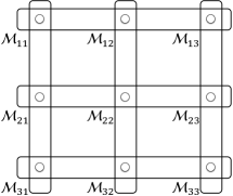
Figure 1: The hypergraph representing compatibility relations among the nine binary-outcome measurements.

By the definition of compatibility for measurements, Eq. (7), this implies that for every row and column there exists a measurement that simulates all the measurements on that row or column. We denote the measurement that simulates the triple of measurements in row 1 by $\operatorname{M}_{R_{1}}$, the one that simulates the triple in column 1 by $\operatorname{M}_{C_{1}}$ and so forth. We denote their outcomes by $m_{R_{1}}$, $m_{C_{1}}$, and so forth.

We now turn to the nature of the particular relation that holds between the measurements on a given row or column and the measurement that simulates them. Consider the measurements in the first row. The outcomes of the simulating measurement $m_{R_{1}}$ is presumed to be 4-valued, such that it can be presented as an ordered pair of binary outcomes, which we denote by $m_{R_{1},1}$ and $m_{R_{1},2}$. In terms of this notation, the three measurements in the first row are presumed to be obtained from the simulating measurement by the following identification of outcomes,

$$\mathcal{m}_{11} =m_{R_{1},1}$$ (41a)

$$\mathcal{m}_{12} =m_{R_{1},2}$$ (41b)

$$\mathcal{m}_{13} =m_{R_{1},1}\cdot m_{R_{1},2}.$$ (41c)

which in terms of the conditional probabilities in Eq. (7) corresponds to the following post-processings of the simulating measurement:

$${\rm pr}\{\mathcal{m}_{11}|m_{R_{1}}\} =\delta_{\mathcal{m}_{11},m_{R_{1},1}}$$ (42a)

$${\rm pr}\{\mathcal{m}_{12}|m_{R_{1}}\} =\delta_{\mathcal{m}_{12},m_{R_{1},2}}$$ (42b)

$${\rm pr}\{\mathcal{m}_{13}|m_{R_{1}}\} =\delta_{\mathcal{m}_{13},m_{R_{1},1}\cdot m_{R_{1},2}}.$$ (42c)

Analogous compatibility relations hold for the second and third rows and for the first and second column. The relations are slightly different for the third column:

$$\mathcal{m}_{13} =m_{C_{3},1}$$ (43a)

$$\mathcal{m}_{23} =m_{C_{3},2}$$ (43b)

$$\mathcal{m}_{33} =-m_{C_{3},1}\cdot m_{C_{3},2},$$ (43c)

or in terms of the conditional probabilities,

$${\rm pr}\{\mathcal{m}_{13}|m_{C_{3}}\} =\delta_{\mathcal{m}_{13},m_{C_{3},1}}$$ (44a)

$${\rm pr}\{\mathcal{m}_{23}|m_{C_{3}}\} =\delta_{\mathcal{m}_{23},m_{C_{3},2}}$$ (44b)

$${\rm pr}\{\mathcal{m}_{33}|m_{C_{3}}\} =\delta_{\mathcal{m}_{33},-m_{C_{3},1}\cdot m_{C_{3},2}}.$$ (44c)

A similar story holds for the sources. There are 9 distinct equivalence classes of binary-outcome sources, which we label by $\mathcal{S}_{ij}$ where $i\in\{1,2,3\}$ and $j\in\{1,2,3\}$, with compatibility relations described by the hypergraph of Fig. 2.

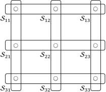
Figure 2: The hypergraph representing compatibility relations among the nine binary-outcome sources.

By the definition of compatibility for sources, Eq. (10), this implies that for every row and column there exists a source that simulates all the sources on that row or column. We denote the source that simulates the triple of measurements in row 1 by $\operatorname{S}_{R_{1}}$ and its outcome by $s_{R_{1}}$, the one that simulates the triple in column 1 by $\operatorname{S}_{C_{1}}$ and its outcome by $s_{C_{1}}$, and so forth. Each such outcome is presumed to be 4-valued, such that it can be presented as an ordered pair of binary variables, so that $s_{R_{1}}=(s_{R_{1},1},s_{R_{1},2})$, etcetera. The conditional probabilities, which, by Eq. (10), define the precise nature of the compatibility relations are exactly the same as for the measurements. For the first row, they are

$${\rm pr}\{\mathcal{s}_{11}|s_{R_{1}}\} =\delta_{\mathcal{s}_{11},s_{R_{1},1}}$$ (45a)

$${\rm pr}\{\mathcal{s}_{12}|s_{R_{1}}\} =\delta_{\mathcal{s}_{12},s_{R_{1},2}}$$ (45b)

$${\rm pr}\{\mathcal{s}_{13}|s_{R_{1}}\} =\delta_{\mathcal{s}_{13},s_{R_{1},1}\cdot s_{R_{1},2}}.$$ (45c)

with analogous relations holding for the other rows and the first and second column, while for the third column, they are

$${\rm pr}\{\mathcal{s}_{13}|s_{C_{3}}\} =\delta_{\mathcal{s}_{13},s_{C_{3},1}}$$ (46a)

$${\rm pr}\{\mathcal{s}_{23}|s_{C_{3}}\} =\delta_{\mathcal{s}_{23},s_{C_{3},2}}$$ (46b)

$${\rm pr}\{\mathcal{s}_{33}|s_{C_{3}}\} =\delta_{\mathcal{s}_{33},-s_{C_{3},1}\cdot s_{C_{3},2}}.$$ (46c)

IV.1.1 Noiseless quantum realization

It is straightforward to verify that the quantum measurements and quantum sources appearing in the no-go theorem described in Sec. III.III.2 instantiate all of the compatibility relations that were described in the previous section.

We begin with the quantum measurements. Take, for example, the three observables in the first row of the Peres-Mermin square. These are associated to the projector-valued measures $\{\Pi_{11}^{(m_{11})}\}_{m_{11}}$, $\{\Pi_{12}^{(m_{12})}\}_{m_{12}}$ and $\{\Pi_{13}^{(m_{13})}\}_{m_{13}}$ where $m_{11},m_{12},m_{13}\in\{-1,+1\}$, each corresponding to the projectors onto the pair of eigenspaces of the corresponding observables, as in Eq. (32). The measurement that simulates all of these is, of course, the one associated to the joint eigenspaces of the three commuting observables, which as a projector-valued measure is $\{\Pi_{R_{1}}^{(m_{R_{1},1},m_{R_{1},2})}\}_{m_{R_{1},1},m_{R_{1},2}}$ where ${(m_{R_{1},1},m_{R_{1},2})\in\{-1,+1\}^{2}}$ and where

$$\begin{split}\Pi_{R_{1}}^{(m_{R_{1},1},m_{R_{1},2})}=\frac{1}{4}\Big{(}&\mathbb{1}\otimes\mathbb{1}+m_{R_{1},1}\operatorname{O}_{11}+m_{R_{1},2}\operatorname{O}_{12}\\ &+(m_{R_{1},1}\cdot m_{R_{1},2})\operatorname{O}_{13}\Big{)}.\end{split}$$ (47)

The simulation of each of the three measurements in the row is achieved by implementing this PVM and then post-processing its outcome using the three conditional probability distributions specified in Eqs. (42a-42c), that is,

$$\Pi_{11}^{(m_{11})} =\smashoperator[]{\sum_{m_{R_{1},1},m_{R_{1},2}}^{}}\delta_{m_{11},m_{R_{1},1}}\Pi_{R_{1}}^{(m_{R_{1},1},m_{R_{1},2})}$$ (48a)

$$\Pi_{12}^{(m_{12})} =\smashoperator[]{\sum_{m_{R_{1},1},m_{R_{1},2}}^{}}\delta_{m_{12},m_{R_{1},2}}\Pi_{R_{1}}^{(m_{R_{1},1},m_{R_{1},2})}$$ (48b)

$$\Pi_{12}^{(m_{13})} =\smashoperator[]{\sum_{m_{R_{1},1},m_{R_{1},2}}^{}}\delta_{m_{13},m_{R_{1},1}\cdot m_{R_{1},2}}\Pi_{R_{1}}^{(m_{R_{1},1},m_{R_{1},2})}.$$ (48c)

In a similar fashion, one can verify that the other rows and columns of the Peres-Mermin square of quantum measurements have the compatibility relations described in the previous section.

The nine quantum sources appearing in the no-go theorem of Sec. III.III.2 also have the compatibility relations described in the previous section. Consider the first row of the source version of the Peres-Mermin square as an example. The three sources on this row are associated to the ensembles $\{\tfrac{1}{2}\rho_{11}^{(s_{11})}\}_{s_{11}}$, $\{\tfrac{1}{2}\rho_{12}^{(s_{12})}\}_{s_{12}}$ and $\{\tfrac{1}{2}\rho_{13}^{(s_{13})}\}_{s_{13}}$ where $s_{11},s_{12},s_{13}\in\{-1,+1\}$, and $\rho_{ij}^{(+)}$ and $\rho_{ij}^{(-)}$ are the normalized projectors onto the eigenspaces of the observables associated to corresponding point on the Peres-Mermin square, as in Eq. (33). The quantum source that simulates all of these is the one associated to the ensemble $\{\tfrac{1}{4}\rho_{R_{1}}^{(s_{R_{1},1},s_{R_{1},2})}\}_{(s_{R_{1},1},s_{R_{1},2})}$, where $\rho_{R_{1}}^{(s_{R_{1},1},s_{R_{1},2})}\equiv\Pi_{R_{1}}^{(s_{R_{1},1},s_{R_{1},2})}$ with $\Pi_{R_{1}}^{(s_{R_{1},1},s_{R_{1},2})}$ the rank-1 projector defined in Eq. (47). The conditional probabilities appearing in the simulation are precisely those given in Eqs. (45a-45c). This fact follows from Eqs. (48a-48c). The compatibility relations for the other rows and columns are verified similarly.

IV.1.2 Noisy quantum realization

In deriving noncontextuality inequalities, it is critical that one not base these on assumptions that are only valid when the measurements or the sources are noiseless because this ideal is never achieved in real experiments. The compatibility relations outlined in Sec. IV.IV.1 satisfy this desideratum. In the quantum case, for instance, they can be satisfied even if the measurements and sources are not sharp (i.e., not associated to an orthogonal set of projectors).

A specific example helps to clarify the point.

Suppose the nine sharp measurements appearing in the Peres-Mermin square are replaced by noisy versions thereof, that is, by the nine unsharp measurements that are the images of the sharp measurements under a partially depolarizing channel $\mathcal{D}$. In this case, the projector-valued measures are replaced by POVMs that are not projective. For instance, the three measurements in the first row of the Peres-Mermin square are associated to the binary-outcome POVMs $\{\mathcal{D}(\Pi_{11}^{(m_{11})})\}_{m_{11}}$, $\{\mathcal{D}(\Pi_{12}^{(m_{12})})\}_{m_{12}}$ and $\{\mathcal{D}(\Pi_{13}^{(m_{13})})\}_{m_{13}}$ where $m_{11},m_{12},m_{13}\in\{-1,+1\}$. These can be jointly implemented using the 4-outcome POVM $\{\mathcal{D}(\Pi_{R_{1}}^{(m_{R_{1},1},m_{R_{1},2})})\}_{m_{R_{1},1},m_{R_{1},2}}$ where $(m_{R_{1},1},m_{R_{1},2})\in\{-1,+1\}^{2}$. The three binary-outcome POVMs are simulated by the 4-outcome POVM using the conditional probabilities in Eqs. (42a-42c); to see this, it suffices to apply $\mathcal{D}$ to Eqs. (48a-48c) and recall that it is a linear map).

Similarly, suppose that the nine sources appearing in the source version of the Peres-Mermin square are replaced by partially depolarized versions thereof. (For simplicitly, we will assume that strength of the noise on the sources is equal to that on the measurements.) In this case, the ensembles associated to the three sources in the first row are $\{\tfrac{1}{2}\mathcal{D}(\rho_{11}^{(s_{11})})\}_{s_{11}}$, $\{\tfrac{1}{2}\mathcal{D}(\rho_{12}^{(s_{12})})\}_{s_{12}}$ and $\{\tfrac{1}{2}\mathcal{D}(\rho_{13}^{(s_{13})})\}_{s_{13}}$ where $s_{11},s_{12},s_{13}\in\{-1,+1\}$. The source that simulates all of these is then simply the partially depolarized version of the one that simulated the sharp sources, that is, $\{\tfrac{1}{4}\mathcal{D}(\rho_{R_{1}}^{(s_{R_{1},1},s_{R_{1},2})})\}_{(s_{R_{1},1},s_{R_{1},2})}$, which again follows from the linearity of Eqs. (48a-48c).

Recall that a partial depolarization map $\mathcal{D}$ can be written as a convex mixture of the identity channel, $\mathcal{I}$, and the channel that traces over the system and reprepares the completely mixed state. An element of the 1-parameter family of such maps is

$$\mathcal{D}_{r}=r\,\mathcal{I}+(1-r)\,\frac{1}{4}\mathbb{1}{\rm Tr},$$ (49)

where $r\in[0,1]$. The strength of depolarization is specified by the probability $r$ of realizing the identity map (with lower values of $r$ corresponding to stronger noise).

It follows that the degree of correlation that can be observed between sources and measurements is a function of $r$. For $r<1$, one no longer achieves the perfect correlations of the noiseless quantum realization, Eqs. 34 and 35, but rather imperfect correlations. Denoting the $r$-depolarized versions of the observables $\operatorname{O}_{ij}$ and the ensembles $\operatorname{\mathcal{E}}_{ij}$ by $\operatorname{O}_{ij}^{(r)}$ and $\operatorname{\mathcal{E}}_{ij}^{(r)}$ respectively, we have

$$\begin{split}\forall i,j:\;\;&pr(\mathcal{m}_{ij},\mathcal{s}_{ij}|\operatorname{O}_{ij}^{(r)},E^{(r)}_{ij})\\ &=\tfrac{1}{2}\operatorname{tr}\left\{\mathcal{D}_{r}\left(\Pi_{ij}^{(\mathcal{m}_{ij})}\right)\mathcal{D}_{r}\left(\rho_{ij}^{(\mathcal{s}_{ij})}\right)\right\}\\ &=\tfrac{1}{2}r^{2}\delta_{\mathcal{m}_{ij},\mathcal{s}_{ij}}~{}.\end{split}$$ (50)

This can be expressed equivalently as

$$\forall i,j: \;\;\langle\mathcal{m}_{ij}\mathcal{s}_{ij}\rangle_{\operatorname{O}_{ij}^{(r)},E^{(r)}_{ij}}=r^{2}.$$ (51)

Because the no-go theorem of Sec. III.III.2 relied on having perfect correlations, it is not applicable to the noisy quantum realization of the operational Peres-Mermin scenario. Nonetheless, one expects that for values of $r$ sufficiently close to 1, a noncontextual model should still be ruled out. The noncontextuality inequalities that we derive confirm this expectation. They are robust to noise in the sense that they can be violated by values of $r$ strictly less than 1. The lower bound on $r$ that they imply is determined in Sec. IV.IV.6.IV.6.2. This bound specifies how much noise one can tolerate in the noisy quantum realization of the Peres-Mermin scenario and still rule out a noncontextual model of the experiment.

IV.2 Expressing operational correlations in terms of noncontextual ontic assignments

Consider an experiment that can realize the nine equivalence classes of measurements and the nine equivalence classes of sources having the compatibility structures of Figs. 1 and 2 respectively and having the compatibility relations specified in the text, such as Eqs. (42a-42c) and Eqs. (45a-45c). There are 81 possible pairings of a source with a measurement. For a given such pairing, say $\mathcal{S}_{ij}$ with $\mathcal{M}_{i^{\prime}j^{\prime}}$, the experiment yields a joint probability distribution over outcomes, $\textrm{pr}(\mathcal{m}_{i^{\prime}j^{\prime}}\mathcal{s}_{ij}|\mathcal{M}_{i^{\prime}j^{\prime}}\mathcal{S}_{ij})$. Equivalently, the experimental data can be summarized by the expectation values $\langle\mathcal{s}_{ij}\rangle_{\mathcal{S}_{i^{\prime}j^{\prime}}}$, $\langle\mathcal{m}_{i^{\prime}j^{\prime}}\rangle_{\mathcal{M}_{ij}}$, and $\langle\mathcal{m}_{i^{\prime}j^{\prime}}\mathcal{s}_{ij}\rangle_{\mathcal{M}_{i^{\prime}j^{\prime}}\mathcal{S}_{ij}}$.

In this article, we limit our focus to deriving constraints which do not refer to the marginal expectations $\langle\mathcal{s}_{ij}\rangle_{\mathcal{S}_{i^{\prime}j^{\prime}}}$ and $\langle\mathcal{m}_{i^{\prime}j^{\prime}}\rangle_{\mathcal{M}_{ij}}$, i.e. we focus on deriving inequalities which refer only to the correlations $\langle\mathcal{s}_{ij}\mathcal{m}_{i^{\prime}j^{\prime}}\rangle_{\mathcal{S}_{ij}\mathcal{M}_{i^{\prime}j^{\prime}}}$. Furthermore, we consider only 9 of the 81 possible pairings of a source with a measurement, namely those wherein the source and the measurement are associated with a common label in their respective compatibility hypergraphs. That is, we hereafter consider only those correlations $\langle\mathcal{s}_{ij}\mathcal{m}_{i^{\prime}j^{\prime}}\rangle_{\mathcal{S}_{ij}\mathcal{M}_{i^{\prime}j^{\prime}}}$ wherein $(i^{\prime},j^{\prime})=(i,j)$. We will derive the necessary and sufficient conditions – with respect to these nine correlations – for an experiment to admit a noncontextual model.

For the equivalence class of measurements $\mathcal{M}_{ij}$, there are two associated measurement procedures, which we denote by $\operatorname{M}_{ij}^{R}$ and $\operatorname{M}_{ij}^{C}$, with outcomes denoted by $m^{R}_{ij}$ and $m^{C}_{ij}$, and which correspond to whether $\mathcal{M}_{ij}$ is implemented jointly with the other measurements in its row or with the other measurements in its column. Similarly, the equivalence class of sources $\mathcal{S}_{ij}$ is associated with two sources, $S^{R}_{ij}$ and $S^{C}_{ij}$, with outcomes denoted by $s^{R}_{ij}$ and $s^{C}_{ij}$. The operational equivalences imply that $\langle s^{R}_{ij}m^{R}_{ij}\rangle_{S_{ij}^{R}M_{ij}^{R}}=\langle s^{R}_{ij}m^{C}_{ij}\rangle_{S_{ij}^{R}M_{ij}^{C}}=\langle s^{C}_{ij}m^{R}_{ij}\rangle_{S_{ij}^{C}M_{ij}^{R}}=\langle s^{C}_{ij}m^{C}_{ij}\rangle_{S_{ij}^{C}M_{ij}^{C}}$, which we can simply denote by $\langle\mathcal{s}_{ij}\mathcal{m}_{ij}\rangle_{\mathcal{S}_{ij}\mathcal{M}_{ij}}$.

Recall Eq. (17), which specifies how correlations such as $\langle s_{ij}m_{ij}\rangle_{S_{ij}M_{ij}}$ are expressed in an ontological model. Under the assumption of measurement noncontextuality, every measurement in the equivalence class $\mathcal{M}_{ij}$ is assigned the same expectation value by the ontic state. Therefore, because $\operatorname{M}_{ij}^{R},\operatorname{M}_{ij}^{C}\in\mathcal{M}_{ij}$, it follows that

$$\langle m^{R}_{ij}\rangle_{\lambda,M_{ij}^{R}}=\langle m^{C}_{ij}\rangle_{\lambda,M_{ij}^{C}}=\langle\mathcal{m}_{ij}\rangle_{\lambda,\mathcal{M}_{ij}}.$$ (52)

In other words, measurement noncontextuality warrants the assumption that the expectation value for the outcome of $\mathcal{M}_{ij}$ does not depend on the measurement context, that is, whether it is implemented with the measurements in the same row or in the same column of Fig. 1. Similarly, under the assumption of preparation noncontextuality, every source in the equivalence class $\mathcal{S}_{ij}$ is assigned the same retrodictive expectation value by the ontic state, such that because $S^{R}_{ij},S^{C}_{ij}\in\mathcal{S}_{ij}$, it follows that

$$\langle s^{R}_{ij}\rangle_{\lambda,S_{ij}^{R}}=\langle s^{C}_{ij}\rangle_{\lambda,S_{ij}^{C}}=\langle\mathcal{s}_{ij}\rangle_{\lambda,\mathcal{S}_{ij}}.$$ (53)

In other words, the expectation value for the outcome of $\mathcal{S}_{ij}$ does not depend on the source context, that is, whether it is implemented with the sources in the same row or in the same column of Fig. 2.

We conclude that

$$\langle\mathcal{s}_{ij}\mathcal{m}_{ij}\rangle_{\mathcal{S}_{ij}\mathcal{M}_{ij}} =\sum_{\lambda\in\Lambda}\langle\mathcal{s}_{ij}\rangle_{\lambda,\mathcal{S}_{ij}}\,\langle\mathcal{m}_{ij}\rangle_{\lambda,\mathcal{M}_{ij}}\,\mu(\lambda|\mathcal{S}_{ij}).$$ (54)

The operational equivalence relations among the sources and the assumption of preparation noncontextuality together imply one further simplification of this expression, namely, that $\mu(\lambda|\mathcal{S}_{ij})$ is independent of $(i,j)$,

$$\forall(iji^{\prime}j^{\prime}):\mu(\lambda|\mathcal{S}_{ij})=\mu(\lambda|\mathcal{S}_{i^{\prime}j^{\prime}})\equiv\mu(\lambda).$$ (55)

To see why this is the case, consider the triple of sources in the first row of Fig. 2, $\mathcal{S}_{11},\mathcal{S}_{12}$ and $\mathcal{S}_{13}$. By assumption, these are each simulatable by a single source, namely, $S_{R_{1}}$, by post-processing its outcome in the manner specified by the compatibility relations, Eqs. (45a-45c). Marginalizing over the outcome of $\mathcal{S}_{11},\mathcal{S}_{12}$ or $\mathcal{S}_{13}$ is simply a further post-processing of $S_{R_{1}}$ and consequently the outcome-marginalized versions of these three sources are each operationally equivalent to the outcome-marginalized version of $S_{R_{1}}$ and therefore operationally equivalent to one another. The assumption of preparation noncontextuality then implies that the distributions over ontic states associated to these, namely that the three ontic state distributions

$$\mu(\lambda|\mathcal{S}_{11}):=\sum_{\mathcal{s}_{11}}\mu(\mathcal{s}_{11},\lambda|\mathcal{S}_{11})$$

$$\mu(\lambda|\mathcal{S}_{12}):=\sum_{\mathcal{s}_{12}}\mu(\mathcal{s}_{12},\lambda|\mathcal{S}_{12})$$

$$\mu(\lambda|\mathcal{S}_{13}):=\sum_{\mathcal{s}_{13}}\mu(\mathcal{s}_{13},\lambda|\mathcal{S}_{13})$$

are equal,

$$\mu(\lambda|\mathcal{S}_{11}) =\mu(\lambda|\mathcal{S}_{12})=\mu(\lambda|\mathcal{S}_{13}).$$ (56)

The same argument repeated for the other rows and the columns yields analogous equalities. Together these imply Eq. (55).

Denoting $\langle\mathcal{m}_{ij}\rangle_{\lambda,\mathcal{M}_{ij}}$ simply as $\langle\mathcal{m}_{ij}\rangle_{\lambda}$ and $\langle\mathcal{s}_{ij}\rangle_{\lambda,\mathcal{S}_{ij}}$ simply as $\langle\mathcal{s}_{ij}\rangle_{\lambda}$, and using Eq. (55), we find that Eq. (54) becomes

$$\langle\mathcal{s}_{ij}\mathcal{m}_{ij}\rangle_{\mathcal{S}_{ij}\mathcal{M}_{ij}} =\sum_{\lambda\in\Lambda}\langle\mathcal{s}_{ij}\rangle_{\lambda}\langle\mathcal{m}_{ij}\rangle_{\lambda}\mu(\lambda).$$ (57)

We pause here to note that this expression for the correlation between the measurement outcome and the source outcome in a noncontextual model has the same form as the expression for the correlation between the measurement outcomes at the two wings of a Bell experiment in a locally causal model of the latter. This provides a particularly intuitive demonstration of the isomorphism between the assumption of local causality and the assumption of preparation noncontextuality for the outcome-marginalized sources articulated in Eq. (55). Note, however, that the assumptions of noncontextuality articulated in Eqs. 52 and 53 cannot be inferred from an assumption of local causality in the corresponding Bell scenario, so that the noncontextuality inequalities that we derive here are not isomorphic to Bell inequalities.

The compatibility relations among the measurements imply constraints on the $\langle m_{ij}\rangle_{\lambda}$. We will refer to any 9-tuple of expectation values, $(\langle m_{11}\rangle_{\lambda},\langle m_{12}\rangle_{\lambda},\dots,\langle m_{33}\rangle_{\lambda})$, satisfying these constraints as a noncontextual ontic assignment to the measurements. We will see that the set of all such 9-tuples defines a polytope in a 9-dimensional space, which we term the noncontextual measurement-assignment polytope. Similarly, the compatibility relations among the sources imply constraints on the $\langle s_{ij}\rangle_{\lambda}$. We will refer to any 9-tuple of expectation values, $(\langle s_{11}\rangle_{\lambda},\langle s_{12}\rangle_{\lambda},\dots,\langle s_{33}\rangle_{\lambda})$, satisfying these constraints as a (retrodictive) noncontextual ontic assignment to the sources. These also form a polytope, which we term the noncontextual source-assignment polytope. The vertices of a polytope, i.e. the extremal noncontextual ontic assignments, can be deduced from that polytope’s defining constraints using standard convex hull algorithms Fukuda and Prodon (1996); Zolotykh (2012); Avis et al. (1997).

Every ontic state $\lambda$ specifies some noncontextual assignment to measurements, but not every noncontextual assignment corresponds to a vertex of the noncontextual measurement-assignment polytope. Nevertheless, those non-vertex noncontextual assignments to measurements can be simulated by a distribution over ontic states that do correspond to vertices: Suppose $\kappa$ is a variable that runs over the vertices of the noncontextual measurement-assignment polytope. Then, for any $\lambda$ in the polytope, there exists a distribution $p(\kappa|\lambda)$ such that

$$\left(\begin{matrix}\langle\mathcal{m}_{11}\rangle_{\lambda}&\langle\mathcal{m}_{12}\rangle_{\lambda}&\langle\mathcal{m}_{13}\rangle_{\lambda}\\ \langle\mathcal{m}_{21}\rangle_{\lambda}&\langle\mathcal{m}_{22}\rangle_{\lambda}&\langle\mathcal{m}_{23}\rangle_{\lambda}\\ \langle\mathcal{m}_{31}\rangle_{\lambda}&\langle\mathcal{m}_{32}\rangle_{\lambda}&\langle\mathcal{m}_{33}\rangle_{\lambda}\end{matrix}\right)\\ =\sum_{\kappa}\left(\begin{matrix}\langle\mathcal{m}_{11}\rangle_{\kappa}&\langle\mathcal{m}_{12}\rangle_{\kappa}&\langle\mathcal{m}_{13}\rangle_{\kappa}\\ \langle\mathcal{m}_{21}\rangle_{\kappa}&\langle\mathcal{m}_{22}\rangle_{\kappa}&\langle\mathcal{m}_{23}\rangle_{\kappa}\\ \langle\mathcal{m}_{31}\rangle_{\kappa}&\langle\mathcal{m}_{32}\rangle_{\kappa}&\langle\mathcal{m}_{33}\rangle_{\kappa}\end{matrix}\right)p(\kappa|\lambda)$$ (58)

where we have presented the 9-tuple as a $3\times 3$ array.

A similar arguments holds for the noncontextual source-assignment polytope. Denoting its vertices by $\kappa^{\prime}$, for any point $\lambda$ in the noncontextual source-assignment polytope, there exists a distribution $p(\kappa^{\prime}|\lambda)$ such that

$$\left(\begin{matrix}\langle\mathcal{s}_{11}\rangle_{\lambda}&\langle\mathcal{s}_{12}\rangle_{\lambda}&\langle\mathcal{s}_{13}\rangle_{\lambda}\\ \langle\mathcal{s}_{21}\rangle_{\lambda}&\langle\mathcal{s}_{22}\rangle_{\lambda}&\langle\mathcal{s}_{23}\rangle_{\lambda}\\ \langle\mathcal{s}_{31}\rangle_{\lambda}&\langle\mathcal{s}_{32}\rangle_{\lambda}&\langle\mathcal{s}_{33}\rangle_{\lambda}\end{matrix}\right)\\ =\sum_{\kappa^{\prime}}\left(\begin{matrix}\langle\mathcal{s}_{11}\rangle_{\kappa^{\prime}}&\langle\mathcal{s}_{12}\rangle_{\kappa^{\prime}}&\langle\mathcal{s}_{13}\rangle_{\kappa^{\prime}}\\ \langle\mathcal{s}_{21}\rangle_{\kappa^{\prime}}&\langle\mathcal{s}_{22}\rangle_{\kappa^{\prime}}&\langle\mathcal{s}_{23}\rangle_{\kappa^{\prime}}\\ \langle\mathcal{s}_{31}\rangle_{\kappa^{\prime}}&\langle\mathcal{s}_{32}\rangle_{\kappa^{\prime}}&\langle\mathcal{s}_{33}\rangle_{\kappa^{\prime}}\end{matrix}\right)p(\kappa^{\prime}|\lambda)$$ (59)

It is useful to introduce a simplified notation for the nine operational correlations in which we are interested, namely,

$$\omega_{ij}\equiv\langle\mathcal{s}_{ij}\mathcal{m}_{ij}\rangle_{\mathcal{S}_{ij}\mathcal{M}_{ij}}.$$ (60)

The set of 9-dimensional vectors $(\omega_{11},\dots,\omega_{33})$ that can arise in an operational theory that admits of a noncontextual ontological model will be termed the noncontextual correlation polytope. Recalling Eq. (57), and representing the $\omega_{ij}$ as a $3\times 3$ array, it is defined in terms of the noncontextual measurement-assignment polytope and the noncontextual source-assignment polytope as follows:

$$\left(\begin{matrix}\omega_{11}&\omega_{12}&\omega_{13}\\ \omega_{21}&\omega_{22}&\omega_{23}\\ \omega_{31}&\omega_{32}&\omega_{33}\end{matrix}\right)$$

$$\begin{split}&=\sum_{\lambda}\left(\begin{matrix}\langle\mathcal{m}_{11}\rangle_{\lambda}&\langle\mathcal{m}_{12}\rangle_{\lambda}&\langle\mathcal{m}_{13}\rangle_{\lambda}\\ \langle\mathcal{m}_{21}\rangle_{\lambda}&\langle\mathcal{m}_{22}\rangle_{\lambda}&\langle\mathcal{m}_{23}\rangle_{\lambda}\\ \langle\mathcal{m}_{31}\rangle_{\lambda}&\langle\mathcal{m}_{32}\rangle_{\lambda}&\langle\mathcal{m}_{33}\rangle_{\lambda}\end{matrix}\right)\\ &\qquad\circ\left(\begin{matrix}\langle\mathcal{s}_{11}\rangle_{\lambda}&\langle\mathcal{s}_{12}\rangle_{\lambda}&\langle\mathcal{s}_{13}\rangle_{\lambda}\\ \langle\mathcal{s}_{21}\rangle_{\lambda}&\langle\mathcal{s}_{22}\rangle_{\lambda}&\langle\mathcal{s}_{23}\rangle_{\lambda}\\ \langle\mathcal{s}_{31}\rangle_{\lambda}&\langle\mathcal{s}_{32}\rangle_{\lambda}&\langle\mathcal{s}_{33}\rangle_{\lambda}\end{matrix}\right)\mu(\lambda),\end{split}$$ (61)

where $\;\circ\;$ denotes the entry-wise product of the arrays (also known as the Hadamard or Schur product).

Substituting Eqs. (58) and (59), we have

$$\left(\begin{matrix}\omega_{11}&\omega_{12}&\omega_{13}\\ \omega_{21}&\omega_{22}&\omega_{23}\\ \omega_{31}&\omega_{32}&\omega_{33}\end{matrix}\right)$$

$$=\sum_{\kappa,\kappa^{\prime}}\left(\begin{matrix}\langle\mathcal{m}_{11}\rangle_{\kappa}\langle\mathcal{s}_{11}\rangle_{\kappa^{\prime}}&\langle\mathcal{m}_{12}\rangle_{\kappa}\langle\mathcal{s}_{12}\rangle_{\kappa^{\prime}}&\langle\mathcal{m}_{13}\rangle_{\kappa}\langle\mathcal{s}_{13}\rangle_{\kappa^{\prime}}\\ \langle\mathcal{m}_{21}\rangle_{\kappa}\langle\mathcal{s}_{21}\rangle_{\kappa^{\prime}}&\langle\mathcal{m}_{22}\rangle_{\kappa}\langle\mathcal{s}_{22}\rangle_{\kappa^{\prime}}&\langle\mathcal{m}_{23}\rangle_{\kappa}\langle\mathcal{s}_{23}\rangle_{\kappa^{\prime}}\\ \langle\mathcal{m}_{31}\rangle_{\kappa}\langle\mathcal{s}_{31}\rangle_{\kappa^{\prime}}&\langle\mathcal{m}_{32}\rangle_{\kappa}\langle\mathcal{s}_{32}\rangle_{\kappa^{\prime}}&\langle\mathcal{m}_{33}\rangle_{\kappa}\langle\mathcal{s}_{33}\rangle_{\kappa^{\prime}}\end{matrix}\right)$$

$$\times p(\kappa,\kappa^{\prime}),$$ (62)

$$\text{where}\quad p(\kappa,\kappa^{\prime})\equiv\sum_{\lambda}p(\kappa|\lambda)p(\kappa^{\prime}|\lambda)\mu(\lambda).$$ (63)

Therefore, the noncontextual correlation polytope is the convex hull of the correlations one obtains for all possible pairings $(\kappa,\kappa^{\prime})$ of a vertex $\kappa$ from the noncontextual measurement-assignment polytope and a vertex $\kappa^{\prime}$ from the noncontextual source-assignment polytope, that is, the convex hull of the 9-tuples $(\langle\mathcal{m}_{11}\rangle_{\kappa}\langle\mathcal{s}_{11}\rangle_{\kappa^{\prime}},\ldots,\langle\mathcal{m}_{33}\rangle_{\kappa}\langle\mathcal{s}_{33}\rangle_{\kappa^{\prime}})$, as one varies over $(\kappa,\kappa^{\prime})$.

Not every pairing of $(\kappa,\kappa^{\prime})$ corresponds to a unique vertex of the noncontextual correlation polytope: The fact that we consider correlations for only 9 source-measurement pairings and not the full set of 81 such pairings, and the fact that we do not consider any of the marginal expectations, implies that (i) more than one choice of $(\kappa,\kappa^{\prime})$ can yield the same 9-tuple of correlations, and (ii) one choice of $(\kappa,\kappa^{\prime})$ can yield a 9-tuple of correlations that lies in the convex hull of the 9-tuples associated to several other choices of $(\kappa,\kappa^{\prime})$. It is therefore convenient to re-express Eq. (IV.IV.2) simply as

$$\left(\begin{matrix}\omega_{11}&\omega_{12}&\omega_{13}\\ \omega_{21}&\omega_{22}&\omega_{23}\\ \omega_{31}&\omega_{32}&\omega_{33}\end{matrix}\right)$$ (64)

$$=\sum_{\gamma}\left(\begin{matrix}\langle\mathcal{m}_{11}\rangle_{\gamma}\langle\mathcal{s}_{11}\rangle_{\gamma}&\langle\mathcal{m}_{12}\rangle_{\gamma}\langle\mathcal{s}_{12}\rangle_{\gamma}&\langle\mathcal{m}_{13}\rangle_{\gamma}\langle\mathcal{s}_{13}\rangle_{\gamma}\\ \langle\mathcal{m}_{21}\rangle_{\gamma}\langle\mathcal{s}_{21}\rangle_{\gamma}&\langle\mathcal{m}_{22}\rangle_{\gamma}\langle\mathcal{s}_{22}\rangle_{\gamma}&\langle\mathcal{m}_{23}\rangle_{\gamma}\langle\mathcal{s}_{23}\rangle_{\gamma}\\ \langle\mathcal{m}_{31}\rangle_{\gamma}\langle\mathcal{s}_{31}\rangle_{\gamma}&\langle\mathcal{m}_{32}\rangle_{\gamma}\langle\mathcal{s}_{32}\rangle_{\gamma}&\langle\mathcal{m}_{33}\rangle_{\gamma}\langle\mathcal{s}_{33}\rangle_{\gamma}\end{matrix}\right)p(\gamma).$$

where instead of ranging over all pairings of $(\kappa,\kappa^{\prime})$ we restrict $\gamma$ to range over the vertices of the noncontextual correlation polytope without loss of generality.

We ultimately seek to derive noncontextuality inequalities, that is, the nontrivial facet inequalities of the noncontextual correlation polytope. We begin by characterizing the noncontextual measurement-assignment polytope and the noncontextual source-assignment polytope. We will see that the nature of the compatibility relations among the measurements/sources determines their respective facet inequalities. From these, we infer the two set of vertices (measurements & sources) using standard convex hull algorithms Fukuda and Prodon (1996); Barber et al. (1996); Zolotykh (2012); Avis et al. (1997). Subsequently, by considering every possible pairing between those two sets of vertices, we determine the set of vertices of the noncontextual correlation polytope. Finally, using standard convex hull algorithms again, we obtain all of the facet inequalities of the noncontextual correlation polytope. The nontrivial facet inequalities define the set of noncontextuality inequalities for our problem. In the following sections, we proceed through these various steps explicitly.

IV.3 Facets of the noncontextual measurement-assignment and noncontextual source-assignment polytopes

We will begin with the measurements. The compatibility relations holding among the measurements in a given row or column must also hold for the response functions representing these in the ontological model. (This is a constraint on any ontological model, rather than one arising from the assumption of measurement noncontextuality. See Sec. V for further discussion.)

Consider the response functions associated to the three equivalence classes of measurements in the first row of Fig. 1. We denote the set of response functions associated to each of these by $\{\xi_{11}(m_{11}|\lambda)\}_{m_{11}}$, $\{\xi_{12}(m_{12}|\lambda)\}_{m_{12}}$ and $\{\xi_{13}(m_{13}|\lambda)\}_{m_{13}}$ where $m_{11},m_{12},m_{13}\in\{-1,+1\}$, and we denote the set of response functions associated to the measurement that simulates these $\{\xi_{R_{1}}(m_{R_{1},1},m_{R_{1},2}|\lambda)\}_{m_{R_{1},1},m_{R_{1},2}}$ where $(m_{R_{1},1},m_{R_{1},2})\in\{-1,+1\}^{2}$. The fact that the simulation is achieved with the three conditional probability distributions specified in Eqs. (42a-42c) implies that

$$\xi_{11}(m_{11}|\lambda) =\smashoperator[]{\sum_{m_{R_{1},1},m_{R_{1},2}}^{}}\delta_{m_{11},m_{R_{1},1}}\xi_{R_{1}}(m_{R_{1},1},m_{R_{1},2}|\lambda)$$ (65a)

$$\xi_{12}(m_{12}|\lambda) =\smashoperator[]{\sum_{m_{R_{1},1},m_{R_{1},2}}^{}}\delta_{m_{12},m_{R_{1},2}}\xi_{R_{1}}(m_{R_{1},1},m_{R_{1},2}|\lambda)$$ (65b)

$$\begin{split}\xi_{12}(m_{13}|\lambda)&=\\ \smashoperator[]{\sum_{m_{R_{1},1},m_{R_{1},2}}^{}}&\delta_{m_{13},m_{R_{1},1}m_{R_{1},2}}\xi_{R_{1}}(m_{R_{1},1},m_{R_{1},2}|\lambda).\end{split}$$ (65c)

Recalling Eq. (13) and Eq. (41), we infer that

$$\begin{split}\langle m_{11}\rangle_{\lambda}=&\,\xi_{R_{1}}(++|\lambda)+\xi_{R_{1}}(+-|\lambda)\\ &-\xi_{R_{1}}(-+|\lambda)-\xi_{R_{1}}(--|\lambda)\end{split}$$ (66a)

$$\begin{split}\langle m_{12}\rangle_{\lambda}=&\,\xi_{R_{1}}(++|\lambda)-\xi_{R_{1}}(+-|\lambda)\\ &+\xi_{R_{1}}(-+|\lambda)-\xi_{R_{1}}(--|\lambda)\end{split}$$ (66b)

$$\begin{split}\langle m_{13}\rangle_{\lambda}=&\,\xi_{R_{1}}(++|\lambda)-\xi_{R_{1}}(+-|\lambda)\\ &-\xi_{R_{1}}(-+|\lambda)+\xi_{R_{1}}(--|\lambda).\end{split}$$ (66c)

Using the fact that $\xi_{R_{1}}$ is a normalized probability distribution,

$$\begin{split}1=&\xi_{R_{1}}(++|\lambda)+\xi_{R_{1}}(+-|\lambda)\\ &+\xi_{R_{1}}(-+|\lambda)+\xi_{R_{1}}(--|\lambda),\end{split}$$ (67)

the relations Eq. (66a-66c,67) can be inverted to write down the probabilities in terms of the expectation values: for $a,b\in\{-1,+1\}$,

$$\xi_{R_{1}}(a,b|\lambda)=\tfrac{1}{4}\left(1+a\langle m_{11}\rangle_{\lambda}+b\langle m_{12}\rangle_{\lambda}+ab\langle m_{13}\rangle_{\lambda}\right).$$

Finally, from the fact that

$$\forall a,b:\;\xi_{R_{1}}(a,b|\lambda)\geq 0,$$ (68)

we infer that $$\forall a,b:$$

$$-a\langle m_{11}\rangle_{\lambda}-b\langle m_{12}\rangle_{\lambda}-ab\langle m_{13}\rangle_{\lambda}\leq 1.$$ (69)

This logic can be repeated for the other rows and the first two columns. For the third column, it is slightly different. We find

$$\xi_{C_{3}}(a,b|\lambda)=\tfrac{1}{4}\left(1+a\langle m_{11}\rangle_{\lambda}+b\langle m_{12}\rangle_{\lambda}-ab\langle m_{13}\rangle_{\lambda}\right)$$

from which we infer that $\forall a,b:$

$$-a\langle m_{11}\rangle_{\lambda}-b\langle m_{12}\rangle_{\lambda}+ab\langle m_{13}\rangle_{\lambda} \leq 1.$$ (70)

In all then, we find that the 9 expectation values $\{\langle m_{ij}\rangle_{\lambda}:(i,j)\in\{1,2,3\}^{2}\}$ must satisfy

$$\begin{split}\forall i&\in\{1,2,3\}:\\ &\langle m_{i1}\rangle_{\lambda}+\langle m_{i2}\rangle_{\lambda}-\langle m_{i3}\rangle_{\lambda}\leq 1,\\ &\langle m_{i1}\rangle_{\lambda}-\langle m_{i2}\rangle_{\lambda}+\langle m_{i3}\rangle_{\lambda}\leq 1,\\ -&\langle m_{i1}\rangle_{\lambda}+\langle m_{i2}\rangle_{\lambda}+\langle m_{i3}\rangle_{\lambda}\leq 1,\\ -&\langle m_{i1}\rangle_{\lambda}-\langle m_{i2}\rangle_{\lambda}-\langle m_{i3}\rangle_{\lambda}\leq 1,\end{split}$$ (71a)

and

$$\begin{split}\forall j&\in\{1,2,3\}:\\ &\langle m_{1j}\rangle_{\lambda}+\langle m_{2j}\rangle_{\lambda}-\eta_{j}\langle m_{3j}\rangle_{\lambda}\leq 1,\\ &\langle m_{1j}\rangle_{\lambda}-\langle m_{2j}\rangle_{\lambda}+\eta_{j}\langle m_{3j}\rangle_{\lambda}\leq 1,\\ -&\langle m_{1j}\rangle_{\lambda}+\langle m_{2j}\rangle_{\lambda}+\eta_{j}\langle m_{3j}\rangle_{\lambda}\leq 1,\\ -&\langle m_{1j}\rangle_{\lambda}-\langle m_{2j}\rangle_{\lambda}-\eta_{j}\langle m_{3j}\rangle_{\lambda}\leq 1,\end{split}$$ (71b)

where $$\eta_{j}=\begin{dcases*}+1&for $j\in\{1,2\}$\\ -1&for $j=3$\end{dcases*}.$$

Note that these inequalities subsume the constraint that $-1\leq\langle m_{ij}\rangle_{\lambda}\leq+1$ for all $i,j$. Eqs. (71a-71b) capture all of the consequences of the compatibility relations for the ontic expectation values. They are the facet inequalities for the noncontextual measurement-assignment polytope.

Similar constraints hold for the nine retrodictive expectation values $\{\langle s_{ij}\rangle_{\lambda}:(i,j)\in\{1,2,3\}^{2}\}$, as we now show.

Consider the the three equivalence classes of sources in the first row of Fig. 2. We will denote the probability distributions associated to each of these by $\mu_{11}(s_{11},\lambda)$, $\mu_{12}(s_{12},\lambda)$, and $\mu_{13}(s_{13},\lambda)$, where $s_{11},s_{12},s_{13}\in\{-1,+1\}$, and the probability distribution associated to the source that simulates these by $\mu_{R_{1}}(s_{R_{1},1},s_{R_{1},2},\lambda)$ where $(s_{R_{1},1},s_{R_{1},2})\in\{-1,+1\}^{2}$. The fact that these sources obey the compatibility relations given in Eqs. (45a-45c) implies that

$$\mu_{11}(s_{11},\lambda) =\smashoperator[]{\sum_{s_{R_{1},1},s_{R_{1},2}}^{}}\delta_{s_{11},s_{R_{1},1}}\mu_{R_{1}}(s_{R_{1},1},s_{R_{1},2},\lambda)$$ (72a)

$$\mu_{12}(s_{12},\lambda) =\smashoperator[]{\sum_{s_{R_{1},1},s_{R_{1},2}}^{}}\delta_{s_{12},s_{R_{1},2}}\mu_{R_{1}}(s_{R_{1},1},s_{R_{1},2},\lambda)$$ (72b)

$$\begin{split}\mu_{13}(s_{13},\lambda)&=\\ \smashoperator[]{\sum_{s_{R_{1},1},s_{R_{1},2}}^{}}&\delta_{s_{13},s_{R_{1},1}s_{R_{1},2}}\mu_{R_{1}}(s_{R_{1},1},s_{R_{1},2},\lambda).\end{split}$$ (72c)

Note that these expressions allow one to confirm the equality of $\sum_{s_{11}}\mu(s_{11},\lambda|\mathcal{S}_{11})$, $\sum_{s_{12}}\mu(s_{12},\lambda|\mathcal{S}_{12})$ and $\sum_{s_{13}}\mu(s_{13},\lambda|\mathcal{S}_{13})$, noted in Eq. (56), via their equality with $\sum_{s_{R_{1},1},s_{R_{1},2}}\mu_{R_{1}}(s_{R_{1},1},s_{R_{1},2},\lambda)$. Recalling Eq. (55), these outcome-marginalized probability distributions are in fact equal to those associated to every other source in the problem, and we have denoted this unique distribution by $\mu(\lambda)$. It follows that we can Bayesian invert all of the terms in Eqs. (72a-72c) by dividing each equation by $\mu(\lambda)$. We thereby obtain

$$\mu_{11}(s_{11}|\lambda) =\smashoperator[]{\sum_{s_{R_{1},1},s_{R_{1},2}}^{}}\delta_{s_{11},s_{R_{1},1}}\mu_{R_{1}}(s_{R_{1},1},s_{R_{1},2}|\lambda)$$ (73a)

$$\mu_{12}(s_{12}|\lambda) =\smashoperator[]{\sum_{s_{R_{1},1},s_{R_{1},2}}^{}}\delta_{s_{12},s_{R_{1},2}}\mu_{R_{1}}(s_{R_{1},1},s_{R_{1},2}|\lambda)$$ (73b)

$$\begin{split}\mu_{13}(s_{13}|\lambda)&=\\ \smashoperator[]{\sum_{s_{R_{1},1},s_{R_{1},2}}^{}}&\delta_{s_{13},s_{R_{1},1}s_{R_{1},2}}\mu_{R_{1}}(s_{R_{1},1},s_{R_{1},2}|\lambda).\end{split}$$ (73c)

Using these relations, together with Eq. (16), we can express the expectation values $\{\langle s_{ij}\rangle_{\lambda}:(i,j)\in\{1,2,3\}^{2}\}$ in terms of the $\mu_{R_{1}}(s_{R_{1},1},s_{R_{1},2}|\lambda)$. By appealing to the fact that $\mu_{R_{1}}$ is a normalized probability distribution, we can invert these equations and then use $\forall a,b:\mu_{R_{1}}(a,b|\lambda)\geq 0$ to obtain inequality constraints on the $\{\langle s_{ij}\rangle_{\lambda}:(i,j)\in\{1,2,3\}^{2}\}$. The analysis proceeds precisely in analogy with the case of measurements, and we obtain:

$$\begin{split}\forall i&\in\{1,2,3\}:\\ &\langle s_{i1}\rangle_{\lambda}+\langle s_{i2}\rangle_{\lambda}-\langle s_{i3}\rangle_{\lambda}\leq 1,\\ &\langle s_{i1}\rangle_{\lambda}-\langle s_{i2}\rangle_{\lambda}+\langle s_{i3}\rangle_{\lambda}\leq 1,\\ -&\langle s_{i1}\rangle_{\lambda}+\langle s_{i2}\rangle_{\lambda}+\langle s_{i3}\rangle_{\lambda}\leq 1,\\ -&\langle s_{i1}\rangle_{\lambda}-\langle s_{i2}\rangle_{\lambda}-\langle s_{i3}\rangle_{\lambda}\leq 1,\end{split}$$ (74a)

and

$$\begin{split}\forall j&\in\{1,2,3\}:\\ &\langle s_{1j}\rangle_{\lambda}+\langle s_{2j}\rangle_{\lambda}-\eta_{j}\langle s_{3j}\rangle_{\lambda}\leq 1,\\ &\langle s_{1j}\rangle_{\lambda}-\langle s_{2j}\rangle_{\lambda}+\eta_{j}\langle s_{3j}\rangle_{\lambda}\leq 1,\\ -&\langle s_{1j}\rangle_{\lambda}+\langle s_{2j}\rangle_{\lambda}+\eta_{j}\langle s_{3j}\rangle_{\lambda}\leq 1,\\ -&\langle s_{1j}\rangle_{\lambda}-\langle s_{2j}\rangle_{\lambda}-\eta_{j}\langle s_{3j}\rangle_{\lambda}\leq 1.\end{split}$$ (74b)

where $$\eta_{j}=\begin{dcases*}+1&for $j\in\{1,2\}$\\ -1&for $j=3$\end{dcases*}.$$

These are the facet inequalities for the noncontextual source-assignment polytope.

Because Eqs. (74a-74b) have the same form as Eqs. (71a-71b), it follows that the noncontextual measurement-assignment polytope has precisely the same form as the noncontextual source-assignment polytope. It suffices, therefore, to characterize just one of them. In the following, we consider the noncontextual measurement-assignment polytope for definiteness.

IV.4 Vertices of the noncontextual measurement-assignment and noncontextual source-assignment polytopes

In this section, we describe the conversion from the facet representation of the noncontextual measurement-assignment polytope, defined by the facet inequalities of Eqs. (71a-71b), to its vertex represenation. We use standard numerical algorithms to do so Fukuda and Prodon (1996); Barber et al. (1996); Zolotykh (2012); Avis et al. (1997), the details of which are provided in Appendix A. In addition to providing a description of this set of vertices, it is our aim here to provide some intuitions about their form.

To begin with, note that all of the points within the noncontextual measurement-assignment polytope are indeterministic assignments – in the sense of violating Eq. (20) – for one or more of the measurements. To see that there are no noncontextual ontic assignments that are deterministic for all of the measurements, it suffices to note that for deterministic assignments, the constraints (71a-71b) simplify to

$$\lfloor\mathcal{m}_{11}\rfloor_{\lambda}\lfloor\mathcal{m}_{12}\rfloor_{\lambda}\lfloor\mathcal{m}_{13}\rfloor_{\lambda} =+1,$$ (75a)

$$\lfloor\mathcal{m}_{21}\rfloor_{\lambda}\lfloor\mathcal{m}_{22}\rfloor_{\lambda}\lfloor\mathcal{m}_{23}\rfloor_{\lambda} =+1,$$ (75b)

$$\lfloor\mathcal{m}_{31}\rfloor_{\lambda}\lfloor\mathcal{m}_{32}\rfloor_{\lambda}\lfloor\mathcal{m}_{33}\rfloor_{\lambda} =+1,$$ (75c)

$$\lfloor\mathcal{m}_{11}\rfloor_{\lambda}\lfloor\mathcal{m}_{21}\rfloor_{\lambda}\lfloor\mathcal{m}_{31}\rfloor_{\lambda} =+1,$$ (75d)

$$\lfloor\mathcal{m}_{12}\rfloor_{\lambda}\lfloor\mathcal{m}_{22}\rfloor_{\lambda}\lfloor\mathcal{m}_{23}\rfloor_{\lambda} =+1,$$ (75e)

$$\lfloor\mathcal{m}_{13}\rfloor_{\lambda}\lfloor\mathcal{m}_{23}\rfloor_{\lambda}\lfloor\mathcal{m}_{33}\rfloor_{\lambda} =-1.,$$ (75f)

where $\lfloor\mathcal{m}_{11}\rfloor_{\lambda}$ denotes a deterministic assignment by ontic state $\lambda$, and that these are equivalent to the constraints specified in Eqs. (30a-30f), which, as noted in Sec. III.III.1 admit no solution.

To get a feeling for how indeterministic noncontextual ontic assignments to the measurements escape contradiction, it is useful to see a concrete example (one that is a vertex of the noncontextual measurement-assignment polytope). We denote it by $\kappa_{1}$. We begin by describing it in terms of probabilistic assignments to the 4-outcome measurements associated to each row and column, rather than in terms of the expectation values for each the nine equivalence classes of binary-outcome measurements, because the correlations that hold between the different binary-outcome measurements are more transparent in this form. Introducing the notation $p(m)=[\alpha]$ as a shorthand for $p(m)=\delta_{m,\alpha}$ and $p(m,m^{\prime})=[\alpha,\beta]$ for $p(m,m^{\prime})=\delta_{m,\alpha}\delta_{m^{\prime},\beta}$, the vertex $\kappa_{1}$ is:

$$\xi_{R_{1}}(m_{R_{1},1},m_{R_{1},2}|\kappa_{1}) =\tfrac{1}{2}[+1,-1]+\tfrac{1}{2}[-1,+1]$$ (76a)

$$\xi_{R_{2}}(m_{R_{2},1},m_{R_{2},2}|\kappa_{1}) =\tfrac{1}{2}[+1,+1]+\tfrac{1}{2}[-1,-1]$$ (76b)

$$\xi_{R_{3}}(m_{R_{3},1},m_{R_{3},2}|\kappa_{1}) =[+1,+1]$$ (76c)

$$\xi_{C_{1}}(m_{C_{1},1},m_{C_{1},2}|\kappa_{1}) =\tfrac{1}{2}[+1,+1]+\tfrac{1}{2}[-1,-1]$$ (76d)

$$\xi_{C_{2}}(m_{C_{2},1},m_{C_{2},2}|\kappa_{1}) =\tfrac{1}{2}[+1,+1]+\tfrac{1}{2}[-1,-1]$$ (76e)

$$\xi_{C_{3}}(m_{C_{3},1},m_{C_{3},2}|\kappa_{1}) =[-1,+1]$$ (76f)

Using Eqs. (65a)-(65c) and analogues thereof, one can compute from these the response functions for each of the nine equivalence classes of binary-outcome measurements. They are

$$\left(\begin{matrix}\xi_{11}(\mathcal{m}_{11}|\kappa_{1})&\xi_{12}(\mathcal{m}_{12}|\kappa_{1})&\xi_{13}(\mathcal{m}_{13}|\kappa_{1})\\ \xi_{21}(\mathcal{m}_{21}|\kappa_{1})&\xi_{22}(\mathcal{m}_{22}|\kappa_{1})&\xi_{23}(\mathcal{m}_{23}|\kappa_{1})\\ \xi_{31}(\mathcal{m}_{31}|\kappa_{1})&\xi_{32}(\mathcal{m}_{32}|\kappa_{1})&\xi_{33}(\mathcal{m}_{33}|\kappa_{1})\end{matrix}\right)$$ (77)

$$=\left(\begin{matrix}\tfrac{1}{2}[+1]+\tfrac{1}{2}[-1]&\;\;\tfrac{1}{2}[+1]+\tfrac{1}{2}[-1]\;\;&[-1]\\ \tfrac{1}{2}[+1]+\tfrac{1}{2}[-1]&\;\;\tfrac{1}{2}[+1]+\tfrac{1}{2}[-1]\;\;&[+1]\\ [+1]&[+1]&[+1]\\ \end{matrix}\right)$$

It is easy to verify that the two ways of defining the value of the response function for $\mathcal{M}_{ij}$ at $\kappa_{1}$ (via simulation by $M_{R_{i}}$ or via simulation by $M_{C_{j}}$) yield the same result, so that this is indeed a noncontextual assignment satisfying the compatibility relations. In terms of expectation values, this assignment corresponds to

$$\left(\begin{matrix}\langle\mathcal{m}_{11}\rangle_{\kappa_{1}}&\langle\mathcal{m}_{12}\rangle_{\kappa_{1}}&\langle\mathcal{m}_{13}\rangle_{\kappa_{1}}\\ \langle\mathcal{m}_{21}\rangle_{\kappa_{1}}&\langle\mathcal{m}_{22}\rangle_{\kappa_{1}}&\langle\mathcal{m}_{23}\rangle_{\kappa_{1}}\\ \langle\mathcal{m}_{31}\rangle_{\kappa_{1}}&\langle\mathcal{m}_{32}\rangle_{\kappa_{1}}&\langle\mathcal{m}_{33}\rangle_{\kappa_{1}}\end{matrix}\right)=\left(\begin{matrix}0&0&-1\\ 0&0&+1\\ +1&+1&+1\\ \end{matrix}\right).$$ (78)

Note that it makes four of the nine measurements outcome-indeterministic.

A second concrete example of a vertex of the polytope, denoted $\kappa_{2}$, is

$$\left(\begin{matrix}\langle\mathcal{m}_{11}\rangle_{\kappa_{2}}&\langle\mathcal{m}_{12}\rangle_{\kappa_{2}}&\langle\mathcal{m}_{13}\rangle_{\kappa_{2}}\\ \langle\mathcal{m}_{21}\rangle_{\kappa_{2}}&\langle\mathcal{m}_{22}\rangle_{\kappa_{2}}&\langle\mathcal{m}_{23}\rangle_{\kappa_{2}}\\ \langle\mathcal{m}_{31}\rangle_{\kappa_{2}}&\langle\mathcal{m}_{32}\rangle_{\kappa_{2}}&\langle\mathcal{m}_{33}\rangle_{\kappa_{2}}\end{matrix}\right)=\left(\begin{matrix}0&0&+1\\ +1&0&0\\ 0&-1&0\\ \end{matrix}\right),$$ (79)

where six of the nine measurements are outcome-indeterministic.

By considering the set of all deterministic processings of the measurements that preserve the compatibility relations holding among these, defined in Appendix B, one can determine the symmetries of the noncontextual measurement-assignment polytope. Specifically, each such deterministic processing induces a bijective mapping of the set of vertices to itself. The full symmetry group is specified in Appendix B. It is straightforward to verify that it can be generated by the following three deterministic processings:

$$\begin{split}\underbrace{\begin{array}[]{c}\langle\mathcal{m}_{11}\rangle_{\kappa}\leftrightarrow\langle\mathcal{m}_{12}\rangle_{\kappa}\\ \langle\mathcal{m}_{21}\rangle_{\kappa}\leftrightarrow\langle\mathcal{m}_{22}\rangle_{\kappa}\\ \langle\mathcal{m}_{31}\rangle_{\kappa}\leftrightarrow\langle\mathcal{m}_{32}\rangle_{\kappa}\\ \end{array}}_{\mathclap{\text{Swap columns }1\leftrightarrow 2}}&,\quad\text{and}\quad\underbrace{\begin{array}[]{c}\langle\mathcal{m}_{21}\rangle_{\kappa}\leftrightarrow\langle\mathcal{m}_{31}\rangle_{\kappa}\\ \langle\mathcal{m}_{22}\rangle_{\kappa}\leftrightarrow\langle\mathcal{m}_{32}\rangle_{\kappa}\\ \langle\mathcal{m}_{23}\rangle_{\kappa}\leftrightarrow\langle\mathcal{m}_{33}\rangle_{\kappa}\\ \end{array}}_{\mathclap{\text{Swap rows }2\leftrightarrow 3}},\\ \text{and}\quad&\underbrace{\begin{array}[]{l}\langle\mathcal{m}_{12}\rangle_{\kappa}\leftrightarrow\langle\mathcal{m}_{21}\rangle_{\kappa}\\ \langle\mathcal{m}_{31}\rangle_{\kappa}\leftrightarrow\langle\mathcal{m}_{31}\rangle_{\kappa}\\ \langle\mathcal{m}_{23}\rangle_{\kappa}\leftrightarrow\langle\mathcal{m}_{32}\rangle_{\kappa}\\ \langle\mathcal{m}_{33}\rangle_{\kappa}\leftrightarrow-\langle\mathcal{m}_{33}\rangle_{\kappa}\\ \end{array}}_{\mathclap{\text{Modified transpose}}}.\end{split}$$ (80)

Note that the number of measurements that are assigned outcomes deterministically is preserved by these symmetry operations. Consequently, our two examples above, Eq. (78) and Eq. (79), are in different symmetry classes. In fact, we find that there are only these two symmetry classes.

The symmetry class wherein six of the nine measurements are indeterministic contains 48 vertices. As $3\times 3$ matrices, they correspond to those with elements in $\{-1,0,+1\}$ having the property that every row and every column contains precisely one non-zero element. The symmetry class wherein four of the nine measurements are indeterministic contains 72 vertices, and corresponds to those $3\times 3$ matrices with elements in $\{-1,0,+1\}$ having a single row of nonzero elements and a single column of nonzero elements such that the overall parity of the row is +1, and the overall parity of the column is $\eta$, where $\eta=-1$ if it is the third column and $\eta=+1$ otherwise.

IV.5 Vertices of the noncontextual correlation polytope

To determine the vertices of the noncontextual correlation polytope from the vertices of the noncontextual measurement-assignment polytope and those of the noncontextual source-assignment polytope, we preserve only those pairings which lead to extremal 9-tuples, as noted above Eq. (64). Specifically, for each of the $120^{2}\!\!=\!\!14,\!400$ pairings $(\kappa,\kappa^{\prime})$, one computes the 9-tuple $(\langle\mathcal{m}_{11}\rangle_{\kappa}\langle\mathcal{s}_{11}\rangle_{\kappa^{\prime}},\ldots,\langle\mathcal{m}_{33}\rangle_{\kappa}\langle\mathcal{s}_{33}\rangle_{\kappa^{\prime}})$. By eliminating duplicate and non-extremal points from this set, we obtain the vertices of the noncontextual correlation polytope.

A concrete example of a vertex of the noncontextual correlation polytope is obtained by pairing the vertex $\kappa_{1}$ of the noncontextual measurement-assignment polytope, described in Eq. (78), with a vertex $\kappa^{\prime}_{1}$ of the noncontextual source-assignment polytope having precisely the same components as $\kappa_{1}$. This pairing yields

$$\left(\begin{matrix}\langle\mathcal{m}_{11}\rangle_{\kappa_{1}}\langle\mathcal{s}_{11}\rangle_{\kappa^{\prime}_{1}}&\langle\mathcal{m}_{12}\rangle_{\kappa_{1}}\langle\mathcal{s}_{12}\rangle_{\kappa^{\prime}_{1}}&\langle\mathcal{m}_{13}\rangle_{\kappa_{1}}\langle\mathcal{s}_{13}\rangle_{\kappa^{\prime}_{1}}\\ \langle\mathcal{m}_{21}\rangle_{\kappa_{1}}\langle\mathcal{s}_{21}\rangle_{\kappa^{\prime}_{1}}&\langle\mathcal{m}_{22}\rangle_{\kappa_{1}}\langle\mathcal{s}_{22}\rangle_{\kappa^{\prime}_{1}}&\langle\mathcal{m}_{23}\rangle_{\kappa_{1}}\langle\mathcal{s}_{23}\rangle_{\kappa^{\prime}_{1}}\\ \langle\mathcal{m}_{31}\rangle_{\kappa_{1}}\langle\mathcal{s}_{31}\rangle_{\kappa^{\prime}_{1}}&\langle\mathcal{m}_{32}\rangle_{\kappa_{1}}\langle\mathcal{s}_{32}\rangle_{\kappa^{\prime}_{1}}&\langle\mathcal{m}_{33}\rangle_{\kappa_{1}}\langle\mathcal{s}_{33}\rangle_{\kappa^{\prime}_{1}}\end{matrix}\right)$$

$$=\left(\begin{matrix}0&0&+1\\ 0&0&+1\\ +1&+1&+1\\ \end{matrix}\right).$$ (81)

Note that this vertex can also be constructed by pairing $\kappa_{3}$ with a corresponding $\kappa^{\prime}_{3}$, where $\kappa_{3}$ is defined as $\kappa_{1}$ per Eq. (78) but with the first two rows permuted, i.e. such that the $-1$ appears in the second row instead of the first. The distinct pairings $(\kappa_{1},\kappa^{\prime}_{1})$ and $(\kappa_{3},\kappa^{\prime}_{3})$ therefore yield duplicate noncontextual correlation points under entry-wise product.

Another vertex of the noncontextual correlation polytope is obtained by pairing the vertex $\kappa_{2}$ of the noncontextual measurement-assignment polytope, desribed in Eq. (79), with a vertex $\kappa^{\prime}_{2}$ of the noncontextual source-assignment polytope having precisely the same components as $\kappa_{2}$:

$$\left(\begin{matrix}\langle\mathcal{m}_{11}\rangle_{\kappa_{2}}\langle\mathcal{s}_{11}\rangle_{\kappa^{\prime}_{2}}&\langle\mathcal{m}_{12}\rangle_{\kappa_{2}}\langle\mathcal{s}_{12}\rangle_{\kappa^{\prime}_{2}}&\langle\mathcal{m}_{13}\rangle_{\kappa_{2}}\langle\mathcal{s}_{13}\rangle_{\kappa^{\prime}_{2}}\\ \langle\mathcal{m}_{21}\rangle_{\kappa_{2}}\langle\mathcal{s}_{21}\rangle_{\kappa^{\prime}_{2}}&\langle\mathcal{m}_{22}\rangle_{\kappa_{2}}\langle\mathcal{s}_{22}\rangle_{\kappa^{\prime}_{2}}&\langle\mathcal{m}_{23}\rangle_{\kappa_{2}}\langle\mathcal{s}_{23}\rangle_{\kappa^{\prime}_{2}}\\ \langle\mathcal{m}_{31}\rangle_{\kappa_{2}}\langle\mathcal{s}_{31}\rangle_{\kappa^{\prime}_{2}}&\langle\mathcal{m}_{32}\rangle_{\kappa_{2}}\langle\mathcal{s}_{32}\rangle_{\kappa^{\prime}_{2}}&\langle\mathcal{m}_{33}\rangle_{\kappa_{2}}\langle\mathcal{s}_{33}\rangle_{\kappa^{\prime}_{2}}\end{matrix}\right)$$

$$=\left(\begin{matrix}0&0&+1\\ +1&0&0\\ 0&+1&0\\ \end{matrix}\right).$$ (82)

By contrast, if we pair $\kappa_{1}$ with $\kappa^{\prime}_{2}$, we obtain a point that is nonextremal in the noncontextual correlation polytope. We find that the noncontextual correlation polytope has 120 vertices.

By considering the deterministic processings of the measurements and sources which preserve the operational Peres-Mermin scenario—that is, the processings which preserve the compatibility relations among the measurements, the compatibility relations among the sources, and the manner in which the sources and the measurements are paired—we can infer the symmetries of the noncontextual correlation polytope, as discussed in Appendix B. Specifically, every such symmetry bijectively maps the set of vertices of this polytope to itself. The full symmetry group is described in Appendix B, and it is straightforward to verify that it can be generated by the following three processings (which we also describe as operations on the $3\times 3$ matrix):

$$\underbrace{\begin{array}[]{c}\langle\mathcal{m}_{11}\rangle_{\gamma}\langle\mathcal{s}_{11}\rangle_{\gamma}\leftrightarrow\langle\mathcal{m}_{12}\rangle_{\gamma}\langle\mathcal{s}_{12}\rangle_{\gamma}\\ \langle\mathcal{m}_{21}\rangle_{\gamma}\langle\mathcal{s}_{21}\rangle_{\gamma}\leftrightarrow\langle\mathcal{m}_{22}\rangle_{\gamma}\langle\mathcal{s}_{22}\rangle_{\gamma}\\ \langle\mathcal{m}_{31}\rangle_{\gamma}\langle\mathcal{s}_{31}\rangle_{\gamma}\leftrightarrow\langle\mathcal{m}_{32}\rangle_{\gamma}\langle\mathcal{s}_{32}\rangle_{\gamma}\\ \end{array}}_{\mathclap{\text{Columns }1\leftrightarrow 2}}$$ (86)

$$\text{ and }\underbrace{\begin{array}[]{c}\langle\mathcal{m}_{21}\rangle_{\gamma}\langle\mathcal{s}_{21}\rangle_{\gamma}\leftrightarrow\langle\mathcal{m}_{31}\rangle_{\gamma}\langle\mathcal{s}_{31}\rangle_{\gamma}\\ \langle\mathcal{m}_{22}\rangle_{\gamma}\langle\mathcal{s}_{22}\rangle_{\gamma}\leftrightarrow\langle\mathcal{m}_{32}\rangle_{\gamma}\langle\mathcal{s}_{32}\rangle_{\gamma}\\ \langle\mathcal{m}_{23}\rangle_{\gamma}\langle\mathcal{s}_{23}\rangle_{\gamma}\leftrightarrow\langle\mathcal{m}_{33}\rangle_{\gamma}\langle\mathcal{s}_{33}\rangle_{\gamma}\\ \end{array}}_{\mathclap{\text{Rows }2\leftrightarrow 3}}$$ (90)

$$\text{ and }\underbrace{\begin{array}[]{l}\langle\mathcal{m}_{11}\rangle_{\gamma}\langle\mathcal{s}_{11}\rangle_{\gamma}\leftrightarrow-\langle\mathcal{m}_{11}\rangle_{\gamma}\langle\mathcal{s}_{11}\rangle_{\gamma}\\ \langle\mathcal{m}_{12}\rangle_{\gamma}\langle\mathcal{s}_{12}\rangle_{\gamma}\leftrightarrow\langle\mathcal{m}_{21}\rangle_{\gamma}\langle\mathcal{s}_{21}\rangle_{\gamma}\\ \langle\mathcal{m}_{13}\rangle_{\gamma}\langle\mathcal{s}_{13}\rangle_{\gamma}\leftrightarrow-\langle\mathcal{m}_{31}\rangle_{\gamma}\langle\mathcal{s}_{31}\rangle_{\gamma}\\ \langle\mathcal{m}_{23}\rangle_{\gamma}\langle\mathcal{s}_{23}\rangle_{\gamma}\leftrightarrow\langle\mathcal{m}_{32}\rangle_{\gamma}\langle\mathcal{s}_{32}\rangle_{\gamma}\\ \langle\mathcal{m}_{33}\rangle_{\gamma}\langle\mathcal{s}_{33}\rangle_{\gamma}\leftrightarrow-\langle\mathcal{m}_{33}\rangle_{\gamma}\langle\mathcal{s}_{33}\rangle_{\gamma}\\ \end{array}}_{\mathclap{\text{Modified transpose}}}$$ (96)

Note that the modified transpose operation appearing in Eq. 110 is distinct from the modified transpose appearing in Eq. 80.

IV.6 Facets of the noncontextual correlation polytope: noncontextuality inequalities

To determine the facet inequalities for the noncontextual correlation polytope from its vertices, we proceed (again) by solving the convex hull problem Fukuda and Prodon (1996); Barber et al. (1996); Zolotykh (2012); Avis et al. (1997), discussed more fully in Appendix A.

Facet inequalities of the noncontextual correlation polytope have the form

$$\sum_{i,j=1}^{3}\alpha_{ij}\omega_{ij}\leq\beta~{}.$$ (97)

where $\{\alpha_{ij}\}_{ij}$ and $\beta$ are integers. Arranging the $\alpha_{ij}$ and the $\omega_{ij}$ into $3\times 3$ matrices and denoting the entry-wise matrix product by $\;\circ\;$ and the sum of the elements of a matrix $A$ by $\textrm{su}(A)$, we can express this as

$$\textrm{su}\left[\left(\begin{matrix}\alpha_{11}&\alpha_{12}&\alpha_{13}\\ \alpha_{21}&\alpha_{22}&\alpha_{23}\\ \alpha_{31}&\alpha_{32}&\alpha_{33}\\ \end{matrix}\right)\circ\left(\begin{matrix}\omega_{11}&\omega_{12}&\omega_{13}\\ \omega_{21}&\omega_{22}&\omega_{23}\\ \omega_{31}&\omega_{32}&\omega_{33}\end{matrix}\right)\right]\leq\beta.$$ (98)

We will refer to the matrix of $\alpha_{ij}$’s as the coefficient matrix for the inequality.

We find that there are 184 inequalities, all of which are expressed using coefficient matrices where $\forall i,j:\alpha_{ij}\in\{0,-1,+1\}$ and where $\beta\in\{1,3,5\}$.

Note that the deterministic processings of the experiment that bijectively map the set of vertices of the noncontextual correlation polytope to itself also bijectively map the set of facet inequalities of the noncontextual correlation polytope to itself, and vice versa. Consequently, the symmetry group of the set of facet inequalities is the same as the symmetry group of the set of vertices. The value of $\beta$ in a facet inequality is invariant under the symmetry group, so that only the matrix of $\alpha$ coefficients transforms nontrivially. Given that the facet inequalities can be expressed in the form of Eq. (98), any map on the $\omega$ matrix can be transferred onto the matrix of $\alpha$ coefficients. Consequently, the action of the symmetry group on the coefficient matrix is precisely parallel to that described in Eq. (86), namely, the group generated by

$$\underbrace{\begin{array}[]{c}\alpha_{11}\leftrightarrow\alpha_{12}\\ \alpha_{21}\leftrightarrow\alpha_{22}\\ \alpha_{31}\leftrightarrow\alpha_{32}\\ \end{array}}_{\mathclap{\text{Columns }1\leftrightarrow 2}}\text{ and }\underbrace{\begin{array}[]{c}\alpha_{21}\leftrightarrow\alpha_{31}\\ \alpha_{22}\leftrightarrow\alpha_{32}\\ \alpha_{23}\leftrightarrow\alpha_{33}\\ \end{array}}_{\mathclap{\text{Rows }2\leftrightarrow 3}}\text{ and }\underbrace{\begin{array}[]{l}\alpha_{11}\leftrightarrow-\alpha_{11}\\ \alpha_{12}\leftrightarrow\alpha_{21}\\ \alpha_{13}\leftrightarrow-\alpha_{31}\\ \alpha_{23}\leftrightarrow\alpha_{32}\\ \alpha_{33}\leftrightarrow-\alpha_{33}\\ \end{array}}_{\mathclap{\text{Modified transpose}}}$$ (110)

Thus, if the $\alpha$ coefficient matrix of one inequality is related to that of another inequality by one of the symmetry operations we have identified, then these two inequalities are in the same symmetry class. An efficient description of all of the facet inequalities is achieved by describing representatives of each of the symmetry classes, and closing under the action of the symmetries. We find that there are just three symmetry classes of facet inequalities, conveniently distinguished by their values of $\beta$.

The first symmetry class is trivial in the sense that the facet inequalities therein hold for all correlations that are logically possible in the operational Peres-Mermin scenario, and consequently they are not sensitive to whether or not the correlations admit of a noncontextual model.

Trivial Class: A representative of this class is

$$\textrm{su}\left[\left(\begin{matrix}-1&+1&+1\\ 0&0&0\\ 0&0&0\\ \end{matrix}\right)\circ\left(\begin{matrix}\omega_{11}&\omega_{12}&\omega_{13}\\ \omega_{21}&\omega_{22}&\omega_{23}\\ \omega_{31}&\omega_{32}&\omega_{33}\end{matrix}\right)\right]\leq 1\,.$$ (111)

Closing under the symmetries, one finds that there are 24 such inequalities, corresponding to coefficient matrices where only one row or column has all nonzero elements, and such that the overall parity of these is $-1$. We justify the claim that these inequalities are trivial in Appendix C.

The term noncontextuality inequality is reserved for those facet inequalities of the noncontextual correlation polytope that are nontrivial. There are two symmetry classes of these.

Nontrivial Class I: A representative of this class is

$$\textrm{su}\left[\left(\begin{matrix}-1&0&+1\\ +1&0&+1\\ 0&-1&0\\ \end{matrix}\right)\circ\left(\begin{matrix}\omega_{11}&\omega_{12}&\omega_{13}\\ \omega_{21}&\omega_{22}&\omega_{23}\\ \omega_{31}&\omega_{32}&\omega_{33}\end{matrix}\right)\right]\leq 3\,.$$ (112)

Closing under the symmetries, one finds that there are 144 such inequalities, all of which can be constructed as follows: Choose a special position in the matrix of coefficients, say element $\alpha_{ij}$, and make it +1 or $-1$. Let all other elements in the same row or column of the coefficients matrix be zero. Finally, choose any assignment of $\pm 1$ for the remaining four elements such that the overall parity of the five nonzero elements is $+1$. The example inequality of Eq. (112) is one of the eight inequalities that follow by starting with $\alpha_{32}=-1$ as the special element.

An example of an inequality from this class that is maximally violated by the noiseless quantum realization of the operational Peres-Mermin scenario (described in Sec. IV.IV.1.IV.1.1) is

$$\textrm{su}\left[\left(\begin{matrix}+1&+1&0\\ +1&+1&0\\ 0&0&+1\\ \end{matrix}\right)\circ\left(\begin{matrix}\omega_{11}&\omega_{12}&\omega_{13}\\ \omega_{21}&\omega_{22}&\omega_{23}\\ \omega_{31}&\omega_{32}&\omega_{33}\end{matrix}\right)\right]\leq 3\,,$$ (113)

as we will demonstrate in the next section.

Nontrivial Class II: A representative of this class is

$$\textrm{su}\left[\left(\begin{matrix}+1&-1&-1\\ +1&+1&+1\\ +1&-1&-1\\ \end{matrix}\right)\circ\left(\begin{matrix}\omega_{11}&\omega_{12}&\omega_{13}\\ \omega_{21}&\omega_{22}&\omega_{23}\\ \omega_{31}&\omega_{32}&\omega_{33}\end{matrix}\right)\right]\leq 5\,.$$ (114)

Closing under the symmetries, one finds that there are 16 inequalities in this class, all of which have only nonzero elements in the coefficient matrix. The 16 inequalities are precisely those whose coefficient matrices have $+1$ overall parity for every row and every column.

An example of an inequality from this class that is maximally violated by the noiseless quantum realization of the operational Peres-Mermin scenario (described in Sec. IV.IV.1.IV.1.1) is

$$\textrm{su}\left[\left(\begin{matrix}+1&+1&+1\\ +1&+1&+1\\ +1&+1&+1\\ \end{matrix}\right)\circ\left(\begin{matrix}\omega_{11}&\omega_{12}&\omega_{13}\\ \omega_{21}&\omega_{22}&\omega_{23}\\ \omega_{31}&\omega_{32}&\omega_{33}\end{matrix}\right)\right]\leq 5\,,$$ (115)

as we will demonstrate in the next section.

IV.6.1 Quantum violation of the inequalities

We have already seen in Sec. III.III.2 that one can identify sharp quantum sources and sharp quantum measurements that satisfy the Peres-Mermin compatibility structure and whose statistics are inconsistent with a universally noncontextual model. These quantum sources and measurements must therefore violate our inequalities. Indeed, for these quantum sources and measurements, it follows from Eq. (35) that $\forall i,j:\omega_{ij}=1$, that is, every one of the nine source-measurement pairs exhibits perfect correlation. This implies that the right-hand side of the noncontextuality inequality of Eq. (113) evaluates to 5 for this quantum realization, thereby exceeding the noncontextual bound of 3. It also implies that the right-hand side of the noncontextuality inequality of Eq. (113) evaluates to 9, which exceeds the noncontextual bound of 5.

IV.6.2 Robustness of the inequalities to noise

We now demonstrate explicitly how the noncontextuality inequalities we have derived are robust to noise by showing that the noisy quantum realization of the operational Peres-Mermin scenario, described in Sec. IV.IV.1.IV.1.2, can still lead to a violation. Recall that this consisted of quantum sources and quantum measurements that were the image under a partial depolarization map of those appearing in the no-go theorem of Sec. III.III.2.

For these noisy sources and measurements, the value of the correlation for each of the nine source-measurement pairs was computed, as a function of the weight $r$ of the identity map in the partial depolarization, in Eq. (51). Translating into the $\omega_{ij}$ notation of Eq. (60), the result is

$$\forall i,j:\omega_{ij}=r^{2}.$$ (116)

Substituting this expression into the noncontextuality inequality of Eq. (113), we obtain

$$5r^{2}\leq 3,$$ (117)

Consequently, as long as the level of noise is such that ${r>\frac{\sqrt{3}}{\sqrt{5}}\simeq 0.77460}$, one has a violation of the noncontextuality inequality. (Lower values of $r$ correspond to stronger noise, so this is an upper bound on the noise.)

Similarly, from the noncontextuality inequality of Eq. (115), we obtain

$$9r^{2}\leq 5.$$ (118)

implying that we require $r>\frac{\sqrt{5}}{\sqrt{9}}\simeq 0.73536$ to see a violation.

Because $\frac{\sqrt{5}}{9}<\frac{\sqrt{3}}{\sqrt{5}}$, the noncontextuality inequality of Eq. (115) can tolerate more noise than that of Eq. (113).

We have shown that our noncontextuality inequalities still admit a violation even in the presence of significant depolarizing noise relative to the ideal quantum realization. As such, the fact that any attempt at an experimental implementation of the ideal quantum sources and measurements inevitably only realizes noisy versions of these is not an obstacle to demonstrating an experimental failure of noncontextuality.

V How to implement an experimental test of these inequalities

The assumption of noncontextuality only has nontrivial consequences if one has experimentally verified that certain operational equivalence relations hold among the measurements and among the sources. This creates a problem for experimental tests of noncontextuality because the definition of operational equivalence for sources is in terms of equivalence of statistics for all measurements, and for measurements it is in terms of equivalence of statistics for all sources, and, strictly speaking, one can never experimentally implement all possible procedures of either type. The problem may be summarized as the physical impossibility of verifying any criterion that involves a universal quantifier. We here explain our view on what is the appropriate attitude to take towards this problem.

A tomographically-complete set of measurements is defined as a set of measurements whose statistics are sufficient to infer the statistics of any other measurement. A tomographically-complete set of sources is defined as a set of sources whose statistics are sufficient to infer the statistics of any other source. It follows that to judge operational equivalence relations among sources, it is sufficient to consider their statistics on a tomographically-complete set of measurements rather than on all measurements, and to judge operational equivalence relations among measurements, it is sufficient to consider their statistics on a tomographically-complete set of sources rather than on all sources. The problem therefore reduces to identifying tomographically complete sets for each.

It is well known that in quantum theory, the set of observables obtained by taking all products of Pauli operators corresponds to a tomographically complete set of measurements for a pair of qubits. Therefore, quantum theory dictates that one must supplement the products of Pauli operators appearing in the Peres-Mermin square with all the other nontrivial products of Pauli operators, that is, with $\{Y\otimes X,Y\otimes Z,Y\otimes\mathbb{1},\mathbb{1}\otimes Y,X\otimes Y,Z\otimes Y\}$, in order to obtain a tomographically complete set. Consequently, by the lights of quantum theory, in order to test operational equivalence relations among the sources, it is necessary to do more measurements than appear in the Peres-Mermin square construction.

Furthermore, if one seeks to implement a direct experimental test of noncontextuality, then one does not want to presume the correctness of quantum theory. As such, it is inappropriate to presume that the fifteen binary-outcome measurements that one expects to be tomographically complete by the lights of quantum theory are in fact tomographically complete. Instead, one should accumulate experimental evidence for this hypothesis by implementing the greatest diversity of measurements on the system that one can and by verifying that the statistics for each such measurement can be inferred from the statistics of the hypothetical tomographically complete set.

Similar comments apply for the problem of identifying a tomographically complete set of sources for the purpose of evaluating operational equivalence relations among the measurements.

We refer the reader to Ref. Mazurek et al. for more details on how to acquire experimental evidence for a given set of measurements (preparations) being tomographically complete.

Even given good evidence of tomographic completeness, one faces another problem with experimentally verifying operational equivalences, namely, that if one aims to implement a particular set of procedures (termed the target procedures), the unavoidable imprecision of experimental implementations implies that one inevitably fails to do so precisely, and one’s experiment instead realizes a set of procedures that deviate from the target procedures, termed the primary procedures. Given the failure of the primary procedures to coincide with the target procedures, operational equivalence relations that hold among the target procedures need not hold among the primary procedures. The primary procedures therefore do not generally realize the operational equivalence relations that are the starting point for derivations of noncontextuality inequalities. This has been termed the problem of “no strict operational equivalences” in Ref. Mazurek et al. (2016).

Before describing how to resolve it, we specify how it arises in the context of the Peres-Mermin construction.

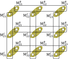
Figure 3: The hypergraph representing compatibility and operational equivalence relations among the eighteen measurements $\{\operatorname{M}_{ij}^{R}\}_{ij}\cup\{\operatorname{M}_{ij}^{C}\}_{ij}$ defined in the text.

There are eighteen target measurement procedures, corresponding to six compatible triples of binary-outcome measurements, one triple for each row and column of the square. Recall that we denoted the 4-outcome measurement that simulates all of the binary-outcome measurements in the first row by $\operatorname{M}_{R_{1}}$ and its outcome by the pair of binary-outcome variables $(m_{R_{1},1},m_{R_{1},2})$. Recall also that we defined $\operatorname{M}_{11}^{R}$ to be the binary-outcome measurement procedure one obtains by implementing $\operatorname{M}_{R_{1}}$ and outputting the single binary variable $m^{R}_{11}=m_{R_{1},1}$ (i.e., by marginalizing over $m_{R_{1},2}$). Similarly, we defined $\operatorname{M}_{11}^{C}$ to be the binary-outcome measurement procedure that one obtains by implementing $M_{C_{1}}$ and outputing the single binary variable $m^{C}_{11}=m_{C_{1},1}$ (i.e., by marginalizing over $m_{C_{1},2}$). $\operatorname{M}_{11}^{R}$ and $\operatorname{M}_{11}^{C}$ are two of the target procedures. Although they are distinct in the sense of involving different physical operations in the laboratory, they are requried to be operationally equivalent in order for the assumption of noncontextuality to have any nontrivial consequences. Similar comments hold for the pair of procedures associated to each of the other points of the Peres-Mermin square. Consequently, if instead of considering the hypergraph where the nodes are operational equivalence classes of measurement procedures and the hyperedges are compatibility relations as we did in Fig. 1, we consider the hypergraph where the nodes are individual measurements, and there are two types of hyperedges, one denoting compatibility relations and the other denoting operational equivalence relations, then we can represent the set of target measurement procedures by Fig. 3.

Note that all of the relationships of compatibility that hold among the measurements are guaranteed by the manner in which those measurements are implemented. Specifically, for every set of compatible measurements in the experiment, these are implemented by various coarse-grainings of a single measurement. As such, the compatibility relations are ensured by construction, and no further evidence must be accumulated to confirm their presence. Only the operational equivalence relations among these different coarse-grained measurements must be tested explicitly.

This distinguishes our approach from other approaches to experimental tests of noncontextuality Kirchmair et al. (2009) wherein the compatibility relations must be tested explicitly. In the latter approaches, the experiment seeks to implement a single measurement procedure $\operatorname{M}$ before or after another measurement $\operatorname{M}^{\prime}$ which is drawn from a set of possibilities that are compatible with $\operatorname{M}$ but incompatible with one another. It is then critical to demonstrate that the procedures $\operatorname{M}$ and $\operatorname{M}^{\prime}$ that are actually realized in the experiment are indeed compatible.

Similar comments apply to sources. In a hypergraph where the nodes are individual sources, and there are two types of hyperedges, one denoting compatibility relations and the other denoting operational equivalence relations, we represent the set of target sources by Fig 4. If every set of compatible sources is implemented by a coarse-graining of a single source, then the compatibility relations among the sources are achieved by construction and only the operational equivalence relations need to be tested.

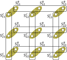
Figure 4: The hypergraph representing compatibility and operational equivalence relations among the eighteen sources $\{\operatorname{S}_{ij}^{R}\}_{ij}\cup\{\operatorname{S}_{ij}^{C}\}_{ij}$ defined in the text.

We are now in a position to describe the problem of no strict operational equivalences in the case of Peres-Mermin. Given the unavoidable deviation of the actually-realized procedures (the primary procedures) from the target procedures, one expects that for each $ij$, the actually-implemented versions of $\operatorname{M}_{ij}^{R}$ and of $\operatorname{M}_{ij}^{C}$ will not be strictly operationally equivalent, nor will the actually-implemented versions of $\operatorname{S}_{ij}^{R}$ and of $\operatorname{S}_{ij}^{C}$.

The resolution to this problem was provided in Ref. Mazurek et al. (2016) and proceeds as follows. When one’s experiment realizes a finite set of primary procedures, it simultaneously provides a characterization of an infinite set of procedures, namely, those that can be obtained by classical post-processing of the set of primary procedures, for instance, any procedure in the convex hull of these. One can then choose a set of secondary procedures from among this infinite set under the constraint of exactly satisfying the desired operational equivalence relations.

Specifically, we select secondary versions of the 4-outcome measurements and 4-outcome sources, under the constraint that the binary-outcome measurements and sources that they define precisely satisfy the operational equivalence relations depicted in the hypergraphs of Figs. 3 and 4 respectively.

Once this is done, one uses the secondary versions of the nine binary-outcome measurements and nine binary-outcome sources to compute the correlations $\{\omega_{ij}\}_{ij}$. Because the operational equivalences hold for these secondary measurements and sources, the assumption of noncontextuality implies a constraint on their ontological representation, and consequently the operational correlations exhibited by these secondary measurements and sources are expected to satisfy the noncontextuality inequalities if the experiment admits of a noncontextual model. A violation of these inequalities by the secondary procedures, therefore, witnesses a failure of noncontextuality.

VI Conclusions

In this paper, we have derived a set of noncontextuality inequalities based on the Peres-Mermin square proof of the impossibility of a KS-noncontextuality in quantum theory. These inequalities are robust to noise and consequently they can be tested directly by experiment. If they are found to be violated by experiment, then not only quantum theory, but any physical theory that can do justice to the experimental data must fail to admit of a noncontextual model. The procedure we have outlined for deriving such inequalities is quite general and can be applied to other state-independent proofs of the Kochen-Specker theorem, particularly those that are expressed algebraically.

In Appendix D, we contrast our approach with previous attempts at deriving operationally-meaningful noncontextuality inequalities based on the Peres-Mermin square and we criticize the latter.

The technique we have described here can be applied to deriving inequalities for correlations in the full set of 81 source-measurement pairings, or even to deriving inequalities on these together with the nine marginal expectation values for the measurements alone and the nine marginal expectation values for the sources alone. What prevented us from doing so here was the computational infeasibility of solving the associated convex hull problems, using the best algorithms for this problem that we could identify and given the computational resources we devoted to the task. It is conceivable, however, that by leveraging our knowledge of the symmetries of the polytopes involved in the problem, one might render it computationally feasible using the same algorithms and computational resources. We are also hopeful that the graph-theoretic techniques for analyzing contextuality scenarios, described in Refs. Cabello et al. (2014); Acín et al. (2015); Kunjwal et al. (2014), might suggest better algorithms for deriving these inequalities.

It is worth noting that the technique for deriving noncontextuality inequalities we have introduced here, insofar as it reduces to a convex hull problem, is an instance of the problem of quantifier elimination. Recent work in quantum foundations has seen increasing use of quantifier elimination algorithms. Fourier-Motzkin elimination, which is appropriate for problems wherein the dependence on the variables to be eliminated is linear, has been used to derive Bell inequalities Budroni and Cabello (2012), and also recently, to derive Bell-like inequalities for novel causal scenarios Chaves et al. (2014); Chaves (2016); Wolfe et al. (2016). In Ref. Wolfe et al. (2016), where the problem is reduced to what is known as the classical marginals problem—that of determining whether a given set of distributions on various subsets of a set of variables can arise as the marginals of a single joint distribution over all of the variables—and this problem can be solved by performing quantifier elimination on the probabilities in the joint distributions using convex hull algorithms. Nonlinear quantifier elimination using computational algebraic geometry has also found application in deriving Bell-like inequalities in simple scenarios Lee and Spekkens (2015). We anticipate that these more general techniques for quantifier elimination will ultimately also find applications to the derivation of noncontextuality inequalities.

Appendix A Polytope Representation Conversion

The problem of converting between polytope representations is essential to our technique for deriving noncontextuality inequalities. We describe the abstract mathematical problem here, and refer the reader to various software packages which are capable of solving it efficiently. A polytope may be uniquely characterized in terms of two dual descriptions: (1) as a collection of facet-defining inequalities, which is called the halfspace representation of the polytope, denoted H-rep, or (2) as a collection of vertices, which is called the vertex representation of the polytope, denoted V-rep. It turns out that facet enumeration from vertices and vertex enumeration from facets are exactly the same computational problem. To understand the representation conversion problem in general, it is imperative to first understand the computational data structures used to represent a collection of points or a collection of inequalities pertaining to $d$-dimensional vector spaces.

We elect to represent the inequality

$$0\leq c_{0}+\sum\limits_{i=1}^{d}c_{i}x_{i}$$

by the $(d+1)$-dimensional vector

$$\bm{h}:=\,\left\{\frac{c_{0}}{g},\frac{c_{1}}{g},...,\frac{c_{d}}{g}\right\}$$

where $g$ is chosen to efficiently store $\bm{h}$ in computer memory. For rational coefficients, taking $g=\mbox{GCD}[c_{0},...,c_{d}]$ allows $\bm{h}$ to be stored as a vector of integers. Indeed, for the sort of contextuality problems that involve linear rational compatibility relationships (such as the operational Peres-Mermin scenario), we can always represent the pertinent inequalities by vectors of integers.

We elect to represent the point

$$\bm{x}:=\,\left\{x_{1},...,x_{d}\right\}$$

by the $$(d+1)$$-dimensional vector

$$\bm{v}:=\,\left\{\frac{1}{g^{\prime}},\frac{x_{1}}{g^{\prime}},...,\frac{x_{d}}{g^{\prime}}\right\}$$

where $g^{\prime}$ is chosen to efficiently store $\bm{v}$ in computer memory. For rational components, taking ${g^{\prime}=\mbox{GCD}[x_{1},...,x_{d}]}$ allows $\bm{v}$ to be stored as a vector of integers.

If a polytope has $n$ facet inequalities, then given that each of these can be represented by a ${(d\!+\!1)}$-dimensional vector, its halfspace representation can be given as an ${n\!\times\!(d\!+\!1)}$ matrix

$$\bm{H}:=\begin{pmatrix}\bm{h}^{(1)}\\ \vdots\\ \bm{h}^{(n)}\end{pmatrix}.$$ (A.1)

We refer to $\bm{H}=\{{\bm{h}}^{(i)}\}_{i}$ as the H-rep matrix.

Similarly, if a polytope has $m$ vertices, then given that each of these can be represented by a ${(d\!+\!1)}$-dimensional vector, its vertex representation can be given as an ${m\!\times\!(d\!+\!1)}$ matrix

$$\bm{V}:=\begin{pmatrix}\bm{v}^{(1)}\\ \vdots\\ \bm{v}^{(m)}\end{pmatrix}.$$ (A.2)

We refer to $\bm{V}=\{{\bm{v}}^{(j)}\}_{j}$ as the V-rep matrix.

It follows that a facet enumeration algorithm takes a V-rep matrix as input and returns an H-rep matrix as output, while a vertex enumeration algorithm takes an H-rep matrix as input and returns a V-rep matrix as output. We now show that the algorithms are equivalent.

A set of point-vectors ${\bm{V}}=\{{\bm{v}}^{(j)}\}_{j}$ defines the V-rep of a polytope relative to some H-rep inequalities-matrix ${\bm{H}}=\{{\bm{h}}^{(i)}\}_{i}$ if and only if the following conditions hold:

Consistent

Every element of $\{{\bm{v}}^{(j)}\}_{j}$ must satisfy all of the facet inequalities,

${\forall i,j:\bm{h}^{(i)}\cdot\bm{v}^{(j)}\geq 0}$.

Complete

Every point ${\bm{x}}$ which cannot be expressed as a positive combination of the elements of $\{{\bm{v}}^{(j)}\}_{j}$ must violate some facet inequality,

$\forall{\bm{x}\not\in\operatorname{PosLinSpan}\left[\{{\bm{v}}^{(j)}\}_{j}\right]}\,,\exists_{i}:\,\bm{h}^{(i)}\cdot\bm{x}<0$.

Concise

No element of $\{{\bm{v}}^{(j)}\}_{j}$ is a positive combination of the others,

${\forall j:\,\bm{v}^{(j)}\not\in\operatorname{PosLinSpan}\left[\{{\bm{v}}^{(k)}\}_{k\neq j}\right]}$.

A set of inequality-vectors ${\bm{H}}=\{{\bm{h}}^{(i)}\}_{i}$ defines the H-rep of a polytope relative to some V-rep vertices-matrix ${\bm{V}}=\{{\bm{v}}^{(j)}\}_{j}$ if and only if the following conditions hold:

Consistent

Every inequality in the set $\{{\bm{h}}^{(i)}\}_{i}$ is satisfied by all of the vertices of the polytope,

${\forall i,j:\bm{h}^{(i)}\cdot\bm{v}^{(j)}\geq 0}$.

Complete

Any inequality ${\bm{c}}$ which cannot be expressed as a positive combination of the inequalities $\{{\bm{h}}^{(i)}\}_{i}$ must be violated by at least one vertex of the polytope,

${\forall{\bm{c}\not\in\operatorname{PosLinSpan}\left[\{{\bm{h}}^{(i)}\}_{i}\right]},\,\exists j:\,\bm{c}\cdot\bm{v}^{(j)}<0}$.

Concise

No inequality in $\{{\bm{h}}^{(i)}\}_{i}$ is a positive combination of the others,

${\forall i:\,\bm{h}^{(i)}\not\in\operatorname{PosLinSpan}\left[\{{\bm{h}}^{(k)}\}_{k\neq i}\right]}$.

It should now be clear that the conditions which define the dual representation are symmetric with respect to the interchange of $\bm{H}$ and $\bm{V}$. Consequently, the polytope representation conversion task is a single computational problem, oblivious to the subjective interpretation of the task as facet enumeration or vertex enumeration. The common underlying computational task is conventionally referred to as the convex hull problem.

In the general procedure for deriving robust operational noncontextuality inequalities, one encounters the convex hull problem three times:

1. When one enumerates the vertices of the noncontextual measurement-assignment polytope starting from its facet inequalities (71a-71b), one is performing H-rep to V-rep conversion.

2. When one enumerates the vertices of the noncontextual source-assignment polytope starting from its facet inequalities (74a-74b), one is performing H-rep to V-rep conversion.

3. When one enumerates the facets of the noncontextual correlation polytope starting from its vertices, one is performing V-rep to H-rep conversion.

For the problem of interest in this article, the Peres-Mermin scenario, the noncontextual measurement-assignment polytope coincides with the noncontextual source-assignment polytope, so the first two instances of the convex hull problem are the same, converting 24 facet inequalities into 120 vertices. The third instance concerns the noncontextual correlation polytope, and converts the 120 vertices thereof into 184 facet inequalities.

Solving the convex hull problem can, in practice, be accomplished by a variety of algorithms; the most prominent implementation is the dual description method. For details on the various algorithms used to solve the convex hull problem see Refs. Fukuda and Prodon (1996); Barber et al. (1996); Zolotykh (2012); Avis et al. (1997). Efficient convex hull solvers are abundant in current software packages.

Note that when we infer the vertices of the noncontextual correlation polytope from the superset of all possible pairings of vertices from the noncontextual measurement-assignment polytope and the noncontextual source-assignment polytope, the computational problem is one of redundancy removal. Redancy removal is the task of isolating the vertices from a set of non-extremal points, or, computationally equivalently, isolating the irredundant linear constraints from some inconcise collection of inequalities. Standard algorithms have been developed for redundancy removal Caron et al. (1989); Matousek (1993), and a variety of current software tools are also available.

Appendix B Deterministic processings of the experimental procedures that preserve the compatiblity relations of the Peres-Mermin scenario

When we express our noncontextuality inequalities in Sec. IV.IV.6, the description of the full set of such inequalities is simplified by appealing to the symmetries of the operational construction. These symmetries correspond to processings of the experiment that permute source-measurement pairs (i.e., deterministically process the setting variables in a correlated fashion), and that deterministically process the outcomes of the measurements and (independently) the outcomes of the sources. It is therefore useful to explicitly characterize these symmetries.

Suppose one has an experiment satisfying the operational features of the Peres-Mermin scenario. This means that there are nine equivalence classes of binary-outcome measurements, $\{\mathcal{M}_{11},\dots,\mathcal{M}_{33}\}$, satisfying the compatibility hypergraph of Fig. 1 and the compatibility relations defined around Eqs. (42a-42c). Similarly, there are nine equivalence classes of binary-outcome sources, $\{\mathcal{S}_{11},\dots,\mathcal{S}_{33}\}$, satisfying the compatibility hypergraph of Fig. 2 and the compatibility relations defined around Eqs. (45a-45c).

Now suppose that from these one defined a new pair of sets, $\{\mathcal{M}^{\prime}_{11},\dots,\mathcal{M}^{\prime}_{33}\}$ and $\{\mathcal{S}^{\prime}_{11},\dots,\mathcal{S}^{\prime}_{33}\}$, as processings of $\{\mathcal{M}_{11},\dots,\mathcal{M}_{33}\}$ and $\{\mathcal{S}_{11},\dots,\mathcal{S}_{33}\}$ as follows. To implement the source-measurement pair $(\mathcal{S}^{\prime}_{ij},\mathcal{M}^{\prime}_{ij})$, one begins by implementing the source-measurement pair $(\mathcal{S}_{\pi(ij)},\mathcal{M}_{\pi(ij)})$, where $\pi$ is some permutation of the nine positions in the Peres-Mermin square, and then for each $\mathcal{M}_{\pi(ij)}$, one multiplies its outcome by $\zeta_{ij}\in\{-1,+1\}$ (thereby either flipping its value or leaving it the same) and for each $\mathcal{S}_{\pi(ij)}$, one multiplies its outcome by $\gamma_{ij}\in\{-1,+1\}$.

The deterministic processings by which the outcomes of the original measurements and sources are mapped to those of the primed measurements and sources can be expressed as follows. Denoting component-wise product of matrices by $\circ$,

$$\left(\begin{matrix}\mathcal{m}^{\prime}_{11}&\mathcal{m}^{\prime}_{12}&\mathcal{m}^{\prime}_{13}\\ \mathcal{m}^{\prime}_{21}&\mathcal{m}^{\prime}_{22}&\mathcal{m}^{\prime}_{23}\\ \mathcal{m}^{\prime}_{31}&\mathcal{m}^{\prime}_{32}&\mathcal{m}^{\prime}_{33}\end{matrix}\right)$$

$$=\left(\begin{matrix}\zeta_{11}&\zeta_{12}&\zeta_{13}\\ \zeta_{21}&\zeta_{22}&\zeta_{23}\\ \zeta_{31}&\zeta_{32}&\zeta_{33}\end{matrix}\right)\circ\left(\begin{matrix}\mathcal{m}_{\pi(11)}&\mathcal{m}_{\pi(12)}&\mathcal{m}_{\pi(13)}\\ \mathcal{m}_{\pi(21)}&\mathcal{m}_{\pi(22)}&\mathcal{m}_{\pi(23)}\\ \mathcal{m}_{\pi(31)}&\mathcal{m}_{\pi(32)}&\mathcal{m}_{\pi(33)}\end{matrix}\right)$$ (B.3)

and

$$\left(\begin{matrix}\mathcal{s}^{\prime}_{11}&\mathcal{s}^{\prime}_{12}&\mathcal{s}^{\prime}_{13}\\ \mathcal{s}^{\prime}_{21}&\mathcal{s}^{\prime}_{22}&\mathcal{s}^{\prime}_{23}\\ \mathcal{s}^{\prime}_{31}&\mathcal{s}^{\prime}_{32}&\mathcal{s}^{\prime}_{33}\end{matrix}\right)$$

$$=\left(\begin{matrix}\gamma_{11}&\gamma_{12}&\gamma_{13}\\ \gamma_{21}&\gamma_{22}&\gamma_{23}\\ \gamma_{31}&\gamma_{32}&\gamma_{33}\end{matrix}\right)\circ\left(\begin{matrix}\mathcal{s}_{\pi(11)}&\mathcal{s}_{\pi(12)}&\mathcal{s}_{\pi(13)}\\ \mathcal{s}_{\pi(21)}&\mathcal{s}_{\pi(22)}&\mathcal{s}_{\pi(23)}\\ \mathcal{s}_{\pi(31)}&\mathcal{s}_{\pi(32)}&\mathcal{s}_{\pi(33)}\end{matrix}\right)$$ (B.4)

We must determine what constraints on $\pi$, $\{\zeta_{ij}\}$ and $\{\gamma_{ij}\}$ are implied by the requirement that the primed measurements have the compatibility relations of the Peres-Mermin scenario.

We begin by deriving some necessary conditions on the permutation $\pi$. To have the right compatibility structure, it is necessary that each of the rows and columns of primed measurements in the Peres-Mermin square (and those of the primed sources) must constitute a compatible triple. It is necessary, therefore, that each must be the image, under the permutation $\pi$, of a compatible triple in the original set of nine measurements (respectively sources), and given that the only triples that are compatible in the original set are the rows and columns, it follows that each must be the image of a row or column of the original. The overall permutation must therefore be generated by permutations of the rows, permutations of the columns, and the transpose of the Peres-Mermin square.

But this condition is not sufficient. We also require the particular compatibility relations among the nine primed measurements (and sources) to be those specified in the operational Peres-Mermin scenario. That is, we require that there exist six 4-outcome measurements $\operatorname{M}_{R_{1}}^{\prime},\operatorname{M}_{R_{2}}^{\prime},\dots,\operatorname{M}_{C_{3}}^{\prime}$ such that primed versions of Eqs. (42a-42c) hold for the first row, and its analogues hold for the other rows and the first two columns, and primed versions of Eqs. (44a-44c) hold for the third column, and we require that there exist six 4-outcome sources $\operatorname{S}_{R_{1}}^{\prime},\operatorname{S}_{R_{2}}^{\prime},\dots,\operatorname{S}_{C_{3}}^{\prime}$ such that primed versions of Eqs. (45a-45c) hold for the first row, and its analogues hold for the other rows and the first two columns, and primed versions of Eqs. (46a-46c) hold for the third column.

We require that for any triple corresponding to a row or a column in the primed Peres-Mermin square, the product of the outcomes in any given run of the experiment must be the same as the product of the outcomes from the corresponding triple in the original square. In other words, the deterministic processing is required to satisfy

$$\mathcal{m}_{a}^{\prime}\mathcal{m}_{b}^{\prime}\mathcal{m}_{c}^{\prime}=\mathcal{m}_{a}\mathcal{m}_{b}\mathcal{m}_{c}.$$ (B.5)

for all $(a,b,c)$ corresponding to compatible triples. Given Eq. (B), it follows that

$$\zeta_{a}\zeta_{b}\zeta_{c}=\frac{\mathcal{m}_{a}\mathcal{m}_{b}\mathcal{m}_{c}}{\mathcal{m}_{\pi(a)}\mathcal{m}_{\pi(b)}\mathcal{m}_{\pi(c)}},$$ (B.6)

Now note that the compatibility relations imply that for each of the nine compatible triples of measurements, the associated triple of outcomes that one can obtain in any run of the experiment has a fixed product, namely,

$$\begin{split}\mathcal{m}_{11}\mathcal{m}_{12}\mathcal{m}_{13}&=+1,\\ \mathcal{m}_{21}\mathcal{m}_{22}\mathcal{m}_{23}&=+1,\\ \mathcal{m}_{31}\mathcal{m}_{32}\mathcal{m}_{33}&=+1,\\ \mathcal{m}_{11}\mathcal{m}_{21}\mathcal{m}_{31}&=+1,\\ \mathcal{m}_{12}\mathcal{m}_{22}\mathcal{m}_{32}&=+1,\\ \mathcal{m}_{13}\mathcal{m}_{23}\mathcal{m}_{33}&=-1.\end{split}$$ (B.7)

(To be clear, we are not here assuming that the particular triple of values that are assigned to, say, $\mathcal{m}_{11},\mathcal{m}_{12},$ and $\mathcal{m}_{13}$, need to be assigned deterministically. Even if the assignment is indeterministic, so that this triple of values is sampled from some probability distribution, the compatibility relations defining the Peres-Meremin construction dictate that only those triples of values that satisfy $\mathcal{m}_{11}\mathcal{m}_{12}\mathcal{m}_{13}=1$ have a nonzero probability of occurrence.)

Consequently, if the permutation $\pi$ is such that the third column is mapped to itself, then for all triples,

$$\zeta_{a}\zeta_{b}\zeta_{c}=+1.$$ (B.8)

If, on the other hand, the permutation $\pi$ maps the third column to a different triple, then

$$\begin{split}&\zeta_{a}\zeta_{b}\zeta_{c}=\begin{dcases}-1&\!\!\!\text{for this distinguished pair of triples}\\ +1&\!\!\!\text{for the other four triples.}\end{dcases}\end{split}$$ (B.9)

The same constraints hold for the $\gamma$’s.

It is useful at this stage to distinguish three sorts of permutations of the Peres-Mermin square. Some notation is required to do so. Let the 2-cycle that interchanges the $(ij)$th element of the square with the $(i^{\prime}j^{\prime})$th element be denoted $((ij)(i^{\prime}j))$. Let the permutation of the first and second row be denoted by $(R_{1}R_{2})$, and similarly for other cases, that is, $(R_{1}R_{2})=((11)(21))((12)(22))((13)(23))$), etcetera. Let the transpose of the Peres-Mermin square be denoted $T$, that is, $T=((13)(31))((12)(21))((23)(32))$. Finally, let the group closure of a set of permutations be denoted “${\rm clos}$”.

The set of all permutations of the Peres-Mermin square that map the third column to itself is:

$$\begin{split}\mathfrak{P}_{A}:=\Big{\{}\pi=&\tilde{\pi}_{C}\pi_{R}:\\ &\pi_{R}\in{\rm clos}\{(R_{1}R_{2}),(R_{2}R_{3})\},\\ &\tilde{\pi}_{C}\in{\rm clos}\{(C_{1}C_{2})\}\Big{\}}.\end{split}$$ (B.10)

Here, $\pi_{R}$ runs over all permutations of the rows, and $\tilde{\pi}_{C}$ is either identity or the swap of the first two columns.

Of those permutations that do not take the third column to itself, it is useful to distinguish those that take it to another column, denoted $\mathfrak{P}_{B}$, and those that take it to a row, denoted $\mathfrak{P}_{C}$. These are defined as follows:

$$\begin{split}\mathfrak{P}_{B}:=\Big{\{}\pi=&\tilde{\pi}_{C}\pi_{R}(C_{2}C_{3}):\\ &\pi_{R}\in{\rm clos}\{(R_{1}R_{2}),(R_{2}R_{3})\},\\ &\tilde{\pi}_{C}\in{\rm clos}\{(C_{1}C_{2})\}\Big{\}},\end{split}$$ (B.11)

where again $\pi_{R}$ runs overs all permutations of the rows, and $\tilde{\pi}_{C}$ is either identity or the swap of the first two columns, and

$$\begin{split}\mathfrak{P}_{C}:=\Big{\{}\pi=&\pi_{C}\pi_{R}:\\ &\pi_{R}\in{\rm clos}\{(R_{1}R_{2}),(R_{2}R_{3})\},\\ &\pi_{C}\in{\rm clos}\{(C_{1}C_{2}),(C_{2}C_{3})\}\Big{\}},\end{split}$$ (B.12)

where $\pi_{R}$ runs overs all permutations of the rows, and $\pi_{C}$ runs over all permutations of the columns.

We can now specify what sorts of deterministic processings of the outcomes (for measurements and for sources) are allowed for each of these types of permutations.

The fact noted at Eq. (B.8) implies that if $\pi\in\mathfrak{P}_{A}$, then the $\zeta$’s must satisfy

$$\begin{split}\zeta_{11}\zeta_{12}\zeta_{13}=+1,\\ \zeta_{21}\zeta_{22}\zeta_{23}=+1,\\ \zeta_{31}\zeta_{32}\zeta_{33}=+1,\\ \zeta_{11}\zeta_{21}\zeta_{31}=+1,\\ \zeta_{12}\zeta_{22}\zeta_{32}=+1,\\ \zeta_{13}\zeta_{23}\zeta_{33}=+1.\end{split}$$ (B.13)

The solutions of these equations include the case of $\zeta_{ij}=+1$ for all $ij$ as well as those of the form

$$\left(\begin{matrix}\zeta_{11}&\zeta_{12}&\zeta_{13}\\ \zeta_{21}&\zeta_{22}&\zeta_{23}\\ \zeta_{31}&\zeta_{32}&\zeta_{33}\end{matrix}\right)=\left(\begin{matrix}-1&-1&+1\\ -1&-1&+1\\ +1&+1&+1\end{matrix}\right)$$ (B.14)

and any matrix of $\zeta$’s obtained from this one by permutation of the rows and columns. The set of such $\zeta$ matrices, denoted $\mathfrak{Z}_{A}$, can be expressed as

$$\begin{split}\mathfrak{Z}_{A}:=\{&(\zeta_{11},\dots,\zeta_{33}):\forall i,j:\zeta_{ij}=+1\}\\ \cup\{&(\zeta_{11},\dots,\zeta_{33}):\exists i\neq i^{\prime},j\neq j^{\prime},\;\\ &\zeta_{ij}=\zeta_{i^{\prime}j}=\zeta_{ij^{\prime}}=\zeta_{i^{\prime}j^{\prime}}=-1,\;\\ &\zeta_{kl}=+1\;{\rm otherwise}\}.\end{split}$$ (B.15)

Precisely the same analysis holds for the $\gamma$’s, so the set of $\gamma$ matrices that preserve the compatibility relations if $\pi\in\mathfrak{P}_{A}$ is also $\mathfrak{Z}_{A}$.

It follows that if

$$(\pi,\{\zeta_{ij}\},\{\gamma_{ij}\})\in\mathfrak{P}_{A}\times\mathfrak{Z}_{A}\times\mathfrak{Z}_{A},$$ (B.16)

then the primed measurements and sources have the compatibility relations of the Peres-Mermin scenario.

Next, consider the case where $\pi\in\mathfrak{P}_{B}$. It is useful to focus on a specific example, namely, $\pi=(C_{2}C_{3})$. The fact noted at Eq. (LABEL:twotriplesminus) implies that the $\zeta$’s must satisfy

$$\begin{split}\zeta_{11}\zeta_{12}\zeta_{13}=+1,\\ \zeta_{21}\zeta_{22}\zeta_{23}=+1,\\ \zeta_{31}\zeta_{32}\zeta_{33}=+1,\\ \zeta_{11}\zeta_{21}\zeta_{31}=+1,\\ \zeta_{12}\zeta_{22}\zeta_{32}=-1,\\ \zeta_{13}\zeta_{23}\zeta_{33}=-1.\end{split}$$ (B.17)

Solutions of these equations are of the form

$$\left(\begin{matrix}\zeta_{11}&\zeta_{12}&\zeta_{13}\\ \zeta_{21}&\zeta_{22}&\zeta_{23}\\ \zeta_{31}&\zeta_{32}&\zeta_{33}\end{matrix}\right)=\left(\begin{matrix}+1&+1&+1\\ +1&+1&+1\\ +1&-1&-1\end{matrix}\right)$$ (B.18)

and any matrix of $\zeta$’s obtained from this one by component-wise multiplication with an element of $\mathfrak{Z}_{A}$. The set of such $\zeta$ matrices, denoted $\mathfrak{Z}_{B}$, can therefore be expressed as

$$\mathfrak{Z}_{B} :=\left\{Z\circ\left(\begin{matrix}+1&+1&+1\\ +1&+1&+1\\ +1&-1&-1\end{matrix}\right):Z\in\mathfrak{Z}_{A}\right\}$$ (B.19)

Similarly, the set of $\gamma$ matrices that preserve the compatibility relations if $\pi\in\mathfrak{P}_{B}$ are those in $\mathfrak{Z}_{B}$.

It follows that if

$$(\pi,\{\zeta_{ij}\},\{\gamma_{ij}\})\in\mathfrak{P}_{B}\times\mathfrak{Z}_{B}\times\mathfrak{Z}_{B},$$ (B.20)

then the primed measurements and sources have the compatibility relations of the Peres-Mermin scenario.

Finally, we consider the third class of permutations, $\mathfrak{P}_{C}$. Again, we begin by focusing on a particular permutation in that class, namely, the transpose, $\pi=T$. The fact noted at Eq. (LABEL:twotriplesminus) implies that in this case the $\zeta$’s must satisfy

$$\begin{split}\zeta_{11}\zeta_{12}\zeta_{13}=+1,\\ \zeta_{21}\zeta_{22}\zeta_{23}=+1,\\ \zeta_{31}\zeta_{32}\zeta_{33}=-1,\\ \zeta_{11}\zeta_{21}\zeta_{31}=+1,\\ \zeta_{12}\zeta_{22}\zeta_{32}=-1,\\ \zeta_{13}\zeta_{23}\zeta_{33}=-1.\end{split}$$ (B.21)

Solutions of these equations are of the form

$$\left(\begin{matrix}\zeta_{11}&\zeta_{12}&\zeta_{13}\\ \zeta_{21}&\zeta_{22}&\zeta_{23}\\ \zeta_{31}&\zeta_{32}&\zeta_{33}\end{matrix}\right)=\left(\begin{matrix}+1&+1&+1\\ +1&+1&+1\\ +1&+1&-1\end{matrix}\right)$$ (B.22)

and any matrix of $\zeta$’s obtained from this one by component-wise multiplication with an element of $\mathfrak{Z}_{A}$. The set of such $\zeta$ matrices, denoted $\mathfrak{Z}_{C}$, is therefore

$$\mathfrak{Z}_{C} :=\left\{Z\circ\left(\begin{matrix}+1&+1&+1\\ +1&+1&+1\\ +1&+1&-1\end{matrix}\right):Z\in\mathfrak{Z}_{A}\right\}$$ (B.23)

The set of $\gamma$ matrices that preserve the compatibility relations if $\pi\in\mathfrak{P}_{C}$ are also those in $\mathfrak{Z}_{C}$.

It follows that if

$$(\pi,\{\zeta_{ij}\},\{\gamma_{ij}\})\in\mathfrak{P}_{C}\times\mathfrak{Z}_{C}\times\mathfrak{Z}_{C},$$ (B.24)

then the primed measurements and sources have the compatibility relations of the Peres-Mermin scenario.

We have now exhaustively enumerated all of the choices of symmetry operations $(\pi,\{\zeta_{ij}\},\{\gamma_{ij}\})$ that preserve the compatibilty relations of the Peres-Mermin scenario. We turn to the question of how these symmetry operations transform the noncontextuality inequalities that we derive.

Recall that our noncontextuality inequalities will ultimately only refer to the following nine products of a measurement outcome variable with its corresponding source outcome variable:

$$\left(\begin{matrix}\mathcal{s}_{11}\mathcal{m}_{11}&\mathcal{s}_{12}\mathcal{m}_{12}&\mathcal{s}_{13}\mathcal{m}_{13}\\ \mathcal{s}_{21}\mathcal{m}_{21}&\mathcal{s}_{22}\mathcal{m}_{22}&\mathcal{s}_{23}\mathcal{m}_{23}\\ \mathcal{s}_{31}\mathcal{m}_{31}&\mathcal{s}_{32}\mathcal{m}_{32}&\mathcal{s}_{33}\mathcal{m}_{33}\end{matrix}\right)$$ (B.25)

If we perform a deterministic processing $(\pi,\{\zeta_{ij}\},\{\gamma_{ij}\})$ then the relevant products of outcome variables for the primed experiment are given by

$$\left(\begin{matrix}\mathcal{s}^{\prime}_{11}\mathcal{m}^{\prime}_{11}&\mathcal{s}^{\prime}_{12}\mathcal{m}^{\prime}_{12}&\mathcal{s}^{\prime}_{13}\mathcal{m}^{\prime}_{13}\\ \mathcal{s}^{\prime}_{21}\mathcal{m}^{\prime}_{21}&\mathcal{s}^{\prime}_{22}\mathcal{m}^{\prime}_{22}&\mathcal{s}^{\prime}_{23}\mathcal{m}^{\prime}_{23}\\ \mathcal{s}^{\prime}_{31}\mathcal{m}^{\prime}_{31}&\mathcal{s}^{\prime}_{32}\mathcal{m}^{\prime}_{32}&\mathcal{s}^{\prime}_{33}\mathcal{m}^{\prime}_{33}\end{matrix}\right)$$

$$\begin{split}&=\left(\begin{matrix}\eta_{11}\zeta_{11}&\eta_{12}\zeta_{12}&\eta_{13}\zeta_{13}\\ \eta_{21}\zeta_{21}&\eta_{22}\zeta_{22}&\eta_{23}\zeta_{23}\\ \eta_{31}\zeta_{31}&\eta_{32}\zeta_{32}&\eta_{33}\zeta_{33}\end{matrix}\right)\\ &\circ\left(\begin{matrix}\mathcal{s}_{\pi(11)}\mathcal{m}_{\pi(11)}&\mathcal{s}_{\pi(12)}\mathcal{m}_{\pi(12)}&\mathcal{s}_{\pi(13)}\mathcal{m}_{\pi(13)}\\ \mathcal{s}_{\pi(21)}\mathcal{m}_{\pi(21)}&\mathcal{s}_{\pi(22)}\mathcal{m}_{\pi(22)}&\mathcal{s}_{\pi(23)}\mathcal{m}_{\pi(23)}\\ \mathcal{s}_{\pi(31)}\mathcal{m}_{\pi(31)}&\mathcal{s}_{\pi(32)}\mathcal{m}_{\pi(32)}&\mathcal{s}_{\pi(33)}\mathcal{m}_{\pi(33)}\end{matrix}\right)\end{split}$$ (B.26)

Note that only the component-wise product of the $\zeta$ matrix and the $\gamma$ matrix is relevant for the products of outcomes of interest. The sets of such products, in each of the three cases considered above, are

$$\begin{split}\mathfrak{D}_{A}&:=\left\{Z\circ Z^{\prime}:Z,Z^{\prime}\in\mathfrak{Z}_{A}\right\},\\ \mathfrak{D}_{B}&:=\left\{Z\circ Z^{\prime}:Z,Z^{\prime}\in\mathfrak{Z}_{B}\right\},\\ \mathfrak{D}_{C}&:=\left\{Z\circ Z^{\prime}:Z,Z^{\prime}\in\mathfrak{Z}_{C}\right\}.\end{split}$$ (B.27)

However, it is straightforward to verify that these three sets are equivalent,

$$\mathfrak{D}_{A}=\mathfrak{D}_{B}=\mathfrak{D}_{C},$$ (B.28)

and easy to determine. They are simply the union of $\mathfrak{Z}_{A}$ and all matrices of the form

$$\left(\begin{matrix}-1&-1&+1\\ -1&+1&-1\\ +1&-1&-1\end{matrix}\right),$$ (B.29)

or obtainable from this one by permutations of the rows and columns.

Appendix C The trivial facet inequalities of the noncontextual correlation polytope

Here we justify the claim that the inequalities in the symmetry class of Eq. (111) are trivial in the sense that they hold for any correlations arising in the operational Peres-Mermin scenario, independently of whether they admit of a noncontextual model or not. Consider the binary-outcome variables defined as products of outcome variables for source-measurement pairs in the first row of the Peres-Mermin square, $\mathcal{s}_{11}\mathcal{m}_{11}$, $\mathcal{s}_{12}\mathcal{m}_{12}$ and $\mathcal{s}_{13}\mathcal{m}_{13}$. Recalling Eqs. (42a-42c), for every run of the experiment we have $\mathcal{m}_{11}\mathcal{m}_{12}\mathcal{m}_{13}=1$, and recalling Eqs. (45a-45c), for each run we have $\mathcal{s}_{11}\mathcal{s}_{12}\mathcal{s}_{13}=1$. This implies that for each run we have $(\mathcal{s}_{11}\mathcal{m}_{11})(\mathcal{s}_{12}\mathcal{m}_{12})(\mathcal{s}_{13}\mathcal{m}_{13})=1$. Given this constraint, it follows that the expectation values of the three variables, $\mathcal{s}_{11}\mathcal{m}_{11}$, $\mathcal{s}_{12}\mathcal{m}_{12}$ and $\mathcal{s}_{13}\mathcal{m}_{13}$, are determined by a joint probability distribution over two of them. But then, positivity of the probabilities in this distribution implies, by an argument articulated around Eqs. 68 and 69, that

$$\begin{split}&\text{for all }a,b\in\{-1,+1\}\,:\\ &-a\langle\mathcal{s}_{11}\mathcal{m}_{11}\rangle-b\langle\mathcal{s}_{12}\mathcal{m}_{12}\rangle-ab\langle\mathcal{s}_{13}\mathcal{m}_{13}\rangle\leq 1.\end{split}$$ (C.30)

Eq. (111) is of this form.

Note that for the third column of the Peres-Mermin square, Eqs. (44a-44c) imply that for every run of the experiment we have $\mathcal{m}_{13}\mathcal{m}_{23}\mathcal{m}_{33}=-1$, and Eqs. (46a-46c) imply that for each run we have $\mathcal{s}_{13}\mathcal{s}_{23}\mathcal{s}_{33}=-1$, but these together yield $(\mathcal{s}_{13}\mathcal{m}_{13})(\mathcal{s}_{23}\mathcal{m}_{23})(\mathcal{s}_{33}\mathcal{m}_{33})=1$, exactly as we have for the other columns and the rows.

Appendix D Criticism of a previous proposal for a noncontextuality inequality based on the Peres-Mermin square

In this section, a prior proposal for an experimental test of noncontextuality based on the Peres-Mermin proof of the Kochen-Specker theorem, that of Cabello Cabello (2008), will be reviewed and criticized. Our criticisms here parallel those provided in Appendix C of Ref. Kunjwal and Spekkens (2015) for a similar proposal that was based on a different proof of the Kochen-Specker theorem.

We describe the proposal of Ref. Cabello (2008) using the notation introduced in this article. There are nine operational quantities appearing in the inequality derived therein, corresponding to the expectation value, relative to an arbitrary preparation $P$, of the product of the outcomes of each of the six triples of compatible measurements in the Peres-Mermin scenario: $\langle\mathcal{m}_{11}\mathcal{m}_{12}\mathcal{m}_{13}\rangle_{P},\langle\mathcal{m}_{21}\mathcal{m}_{22}\mathcal{m}_{23}\rangle_{P},\ldots,\langle\mathcal{m}_{13}\mathcal{m}_{23}\mathcal{m}_{33}\rangle_{P}$. Only the average of these expectation values is considered in Ref. Cabello (2008); we denote it

$$R(P)\equiv\langle\mathcal{m}_{11}\mathcal{m}_{12}\mathcal{m}_{13}\rangle_{P}+\langle\mathcal{m}_{21}\mathcal{m}_{22}\mathcal{m}_{23}\rangle_{P}+\langle\mathcal{m}_{31}\mathcal{m}_{32}\mathcal{m}_{33}\rangle_{P}+\langle\mathcal{m}_{11}\mathcal{m}_{21}\mathcal{m}_{31}\rangle_{P}+\langle\mathcal{m}_{12}\mathcal{m}_{22}\mathcal{m}_{32}\rangle_{P}-\langle\mathcal{m}_{13}\mathcal{m}_{23}\mathcal{m}_{33}\rangle_{P},$$ (D.31)

The inequality derived in Ref. Cabello (2008) is

$$R(P)\leq 4.$$ (D.32)

We dispute the notion that this inequality delimits the boundary between contextual and noncontextual theories, and therefore also the notion that experimental violations thereof, such as those achieved in Refs. Amselem et al. (2009); Liu et al. (2009); D’Ambrosio et al. (2013), have any bearing on the possibility of noncontextual models, for reasons that we presently outline.

We begin by reviewing the argument presented in favour of Eq. (D.32). Ref. Cabello (2008) presumes that outcomes are assigned deterministically by the ontic state. Suppose that $R(\lambda)$ denotes a particular noncontextual deterministic assignment to the sum of the triple-products. Recalling our notational convention that $\lfloor\cdot\rfloor_{\lambda}$ denotes a deterministic assignment (See below Eq. (75f)), we have

$$R(\lambda)\equiv\lfloor\mathcal{m}_{11}\mathcal{m}_{12}\mathcal{m}_{13}\rfloor_{\lambda}+\lfloor\mathcal{m}_{21}\mathcal{m}_{22}\mathcal{m}_{23}\rfloor_{\lambda}+\lfloor\mathcal{m}_{31}\mathcal{m}_{32}\mathcal{m}_{33}\rfloor_{\lambda}+\lfloor\mathcal{m}_{11}\mathcal{m}_{21}\mathcal{m}_{31}\rfloor_{\lambda}+\lfloor\mathcal{m}_{12}\mathcal{m}_{22}\mathcal{m}_{32}\rfloor_{\lambda}-\lfloor\mathcal{m}_{13}\mathcal{m}_{23}\mathcal{m}_{33}\rfloor_{\lambda}.$$ (D.33)

Any preparation procedure $P$ corresponds to a convex sum of such assignments,

$$R(P)=\sum_{\lambda}R(\lambda)\mu(\lambda|P).$$ (D.34)

The inequality of Eq. (D.32) is inferred from the inequality

$$R(\lambda)\leq 4,$$ (D.35)

and the argument presented in favour of the latter is simply this: recalling that each of the nine $\mathcal{m}_{ij}$ is assigned a value in $\{-1,+1\}$ in an outcome-deterministic assignment, there are $2^{9}$ possible joint assignments of values to $(\mathcal{m}_{11},\dots,\mathcal{m}_{33})$, and for each of these, one can verify that $R(\lambda)\leq 4$.

We now explain the problem with this argument. The measurement compatibility relations that serve to define the operational Peres-Mermin scenario, described around Eqs. (42a-42c), imply that for each of the six compatible triples of measurements, the associated triple of outcomes that one can obtain in any run of the experiment has a fixed product. Specifically, this product is $-1$ for the triple corresponding to the third column, and +1 for the other five triples, as noted in Eq. (B.7).

However, for each of the $2^{9}$ joint assignments to $(\mathcal{m}_{11},\dots,\mathcal{m}_{33})$, one can identify a compatible triple which are assigned values that are inconsistent with the compatibility relation that they are meant to satisfy. For instance, the assignment of the +1 outcome to each of the nine measurements fails to give the correct product of outcomes for the third column. In other words, if a set of nine measurements satisfy the compatibility relations of the operational Peres-Mermin construction, then none of the $2^{9}$ joint assignments of outcomes to these measurements are logically possible assignments.

More formally, the fact that the assignments are assumed to be deterministic implies that the assignment to the product of the outcome is the product of the assignments to each outcome, $\lfloor\mathcal{m}_{11}\mathcal{m}_{12}\mathcal{m}_{13}\rfloor_{\lambda}=\lfloor\mathcal{m}_{11}\rfloor_{\lambda}\lfloor\mathcal{m}_{12}\rfloor_{\lambda}\lfloor\mathcal{m}_{13}\rfloor_{\lambda}$, and the compatibility relations that are assumed to hold among the measurements imply that the $(\lfloor\mathcal{m}_{12}\rfloor_{\lambda},\ldots,\lfloor\mathcal{m}_{33}\rfloor_{\lambda})$ must satisfy the constraints of Eqs. (75a-75f), which have no solution.

Furthermore, the compatibility relations imply that for any preparation $P$, whatever triple of compatible measurements one implements, the outcomes always satisfy Eq. (B.7), and therefore the expectation values satisfy these relations as well:

$$\begin{split}\langle\mathcal{m}_{11}\mathcal{m}_{12}\mathcal{m}_{13}\rangle_{P}&=+1,\\ \langle\mathcal{m}_{21}\mathcal{m}_{22}\mathcal{m}_{23}\rangle_{P}&=+1,\\ \langle\mathcal{m}_{31}\mathcal{m}_{32}\mathcal{m}_{33}\rangle_{P}&=+1,\\ \langle\mathcal{m}_{11}\mathcal{m}_{21}\mathcal{m}_{31}\rangle_{P}&=+1,\\ \langle\mathcal{m}_{12}\mathcal{m}_{22}\mathcal{m}_{32}\rangle_{P}&=+1,\\ \langle\mathcal{m}_{13}\mathcal{m}_{23}\mathcal{m}_{33}\rangle_{P}&=-1.\end{split}$$ (D.36)

In other words, just as the observables $\mathbb{1}\otimes\mathbb{1}$ and $-\mathbb{1}\otimes\mathbb{1}$ in quantum theory are trivial insofar as they take the same value for all states, the triple-product of outcomes $\mathcal{m}_{11}\mathcal{m}_{12}\mathcal{m}_{13},\ldots,\mathcal{m}_{13}\mathcal{m}_{23}\mathcal{m}_{33}$ are trivial operational quantities insofar as they take the same value for all preparations. Substituting the identities in Eq. (D.36) into Eq. (D.31), one obtains

$$R(P)=6.$$ (D.37)

Therefore, for any set of measurements satisfying the compatibility relations of the operational Peres-Mermin scenario, one will necessarily find this equality to hold.

In particular, we expect Eq. (D.37) to hold no matter how noisy the measurements are. To see this, it suffices to note that the equalities of Eq. (B.7) hold for any set of noisy measurements satisfying the compatibility relations, and this implies that Eq. (D.37) holds for such measurements as well. For instance, Eqs. (B.7) and (D.37) hold for the noisy quantum realization of the operational Peres-Mermin scenario, described in Sec. IV.IV.1.IV.1.2, for any amount of depolarization noise. Consequently, if measuring $R(P)$ to have a value greater than 4 could constitute evidence for the failure of noncontextuality, then this evidence could be obtained even in the presence of arbitrarily large amounts of noise. This is an indictment of the proposal of Ref. Cabello (2008) because a minimal constraint on any reasonable notion of noncontextuality (first articulated in Ref. Kunjwal and Spekkens (2015)) is that it should not be possible to demonstrate its failure in a completely incoherent experiment.

To summarize then, our criticism is as follows. The inequality $R(P)\leq 4$ should not be expected to hold for any experiment satisfying the compatibility structure of the operational Peres-Mermin scenario, while the equality $R(P)=6$ (and hence the violation of $R(P)\leq 4$) is expected to hold trivially in all such experiments. And this is the case regardless of whether the experiment admits of a noncontextual ontological model. As such, the operational quantity $R(P)$ contains no information about whether or not a noncontextual model can describe the experiment.

The most significant point of contrast between the proposal of this article and that of Ref. Cabello (2008) is that we assume the notion of universal noncontextuality proposed in Ref. Spekkens (2005), rather than the notion of KS-noncontextuality. Because universal noncontextuality, unlike KS-noncontextuality, does not assume outcome determinism, we are led to consider indeterministic noncontextual assignments to the measurements. As we saw above, the fact that there are strictly no deterministic noncontextual assignments respecting the compatibility relations of the operational Peres-Mermin scenario is what makes it futile to attempt to derive constraints on operational statistics from the assumption of such assignments. The assumption is logically ruled out, so an operational test is neither necessary nor conceivable. On the other hand, there are many indeterministic noncontextual assignments that respect the compatibility relations, such as the example provided in Eq. (78). These, therefore, do impose nontrivial constraints on operational statistics, constraints that are encoded in the noncontextuality inequalities that we have derived.