Upper bounds for the spectral function on homogeneous spaces via volume growth

Abstract

We use spectral embeddings to give upper bounds on the spectral function of the Laplace–Beltrami operator on homogeneous spaces in terms of the volume growth of balls. In the case of compact manifolds, our bounds extend the 1980 lower bound of Peter Li [17] for the smallest positive eigenvalue to all eigenvalues. We also improve Li’s bound itself. Our bounds translate to explicit upper bounds on the heat kernel for both compact and noncompact homogeneous spaces.

1 [58J50, 58C40, 43A85, 53C30]35P15

1 Introduction

The spectrum of the (nonnegative) Laplace–Beltrami operator $\Delta_{g}$ associated to a compact Riemannian manifold $(M,g)$ consists of a discrete set of nonnegative eigenvalues, each with a finite-dimensional eigenspace. These eigenvalues rarely admit explicit computation, and hence much work has been devoted to their estimation (see, for example, [10, 2]). To bound the eigenvalues of $\Delta_{g}$ in the present paper, we adapt the method of spectral embedding that was used in [20] to estimate eigenvalues of the discrete Laplacian on a graph. See [23] for a history of other uses of spectral embeddings of manifolds. In particular, we provide new lower bounds on the eigenvalues of the Laplacian on Riemannian manifolds with transitive isometry groups, as well as upper bounds on their heat kernels. All of our bounds come with fully explicit constants.

The estimation of the eigenvalues of $\Delta_{g}$ is equivalent to the estimation of the eigenvalue counting function, $N(\lambda)$. Here, $N(\lambda)$ denotes the dimension of ${\mathcal{H}}_{\lambda}$, the direct sum of the eigenspaces with eigenvalue at most $\lambda$. Denote by $V(r)$ the volume of a ball of radius $r$ in $M$ when $M$ is homogeneous (whether or not $M$ is compact). In the compact case, our main result is the following bound:

Theorem 1.1.

(Theorem 3.1) If $(M,g)$ is compact homogeneous space, then for each $\alpha\in\,(0,\pi/2)$,

$$N(\lambda)\leavevmode\nobreak\ \leq\leavevmode\nobreak\ \frac{\operatorname{\mathsf{vol}}_{g}(M)}{\int_{0}^{\pi/2}V(\theta/\sqrt{\lambda})\sin(2\theta)\,d\theta}\leavevmode\nobreak\ \leq\leavevmode\nobreak\ \frac{\operatorname{\mathsf{vol}}_{g}(M)}{\cos^{2}\alpha\cdot V(\alpha\cdot\lambda^{-1/2})}\,.$$

Peter Li [17] showed that the first nonzero eigenvalue of a general compact homogeneous space satisfies

(1.1) $$\sqrt{\lambda_{1}}\leavevmode\nobreak\ >\leavevmode\nobreak\ \frac{\pi}{2D}\,,$$

where $D$ is the diameter of $(M,g)$. Thus, if $\alpha<\pi/2$, then $\lambda\to V(\alpha\lambda^{-\frac{1}{2}})$ is decreasing for $\lambda\geq\lambda_{1}$. Consequently, Theorem 1.1 implies that if $0<\alpha<\pi/2$, then

(1.2) $$\sqrt{\lambda_{k}}\leavevmode\nobreak\ \geq\leavevmode\nobreak\ \frac{\alpha}{V^{-1}\biggl{(}\frac{\textstyle\vrule width=0.0pt,depth=2.0pt\operatorname{\mathsf{vol}}M}{\textstyle(k+1)\cdot\cos^{\vrule width=0.0pt,height=7.0pt2}\alpha}\biggr{)}}\,,$$

where $0=\lambda_{0}<\lambda_{1}\leq\lambda_{2}\leq\lambda_{3}\leq\cdots$ are the eigenvalues listed in ascending order with multiplicity equal to the dimension of the corresponding eigenspace.

In general, for small $r$, we have $V(r)=\omega_{d}\cdot r^{d}+O(r^{d+2})$, where $d$ is the dimension of $M$ and $\omega_{d}$ is the volume of the unit ball in ${\mathbb{R}}^{d}$. Thus, it is natural to assume that $V(r)\geq c\cdot r^{d}$ for $r\leq r_{0}$. In such a case, Theorem 1.1 yields the following bound:

Corollary 1.2.

Let $(M,g)$ be a compact homogeneous space, and let $r_{0}$ and $c$ be positive numbers. If $V(r)\geq c\cdot r^{d}$ for $r\leq r_{0}$, then for $\lambda\geq(\pi/2r_{0})^{2}$, we have

$$N(\lambda)\leavevmode\nobreak\ \leq\leavevmode\nobreak\ \frac{\operatorname{\mathsf{vol}}(M)}{c\cdot m_{d}}\cdot\lambda^{d/2}\,,$$

where $m_{d}:=\int_{0}^{\pi/2}\theta^{d}\sin(2\theta)\,d\theta$.

Explicit $c$ and $r_{0}$ can be derived from an upper bound $\kappa$ on the sectional curvatures of $(M,g)$ and from the injectivity radius ${\rm inj}(M,g)$. Indeed, for $r\leq{\rm inj}(M,g)$, we have $V(r)\geq V_{\kappa}(r)$, where $V_{\kappa}(r)$ is the volume of the ball of radius $r$ in the simply connected homogeneous space of constant curvature $\kappa$ [12]. In turn, the sectional curvatures of a homogeneous space can be computed in terms of the Lie algebra of its isometry group (see, for example, [6]). The function $V_{\kappa}(r)$ can, of course, be computed explicitly; see, for example, [9, §3.H] or Section 7 here.

The bound in Corollary 1.2 should be compared to Weyl’s Law, the well-known large-$\lambda$ asymptotics of $N(\lambda)$:

(1.3) $$\lim_{\lambda\to\infty}\frac{N(\lambda)}{\lambda^{d/2}}\leavevmode\nobreak\ =\leavevmode\nobreak\ \frac{\omega_{d}\cdot\operatorname{\mathsf{vol}}(M)}{(2\pi)^{d}}\,.$$

Since $V(r)\sim\omega_{d}\cdot r^{d}$ as $r$ tends to zero, Corollary 1.2 yields that

(1.4) $$\limsup_{\lambda\to\infty}\frac{N(\lambda)}{\lambda^{d/2}}\leavevmode\nobreak\ \leq\leavevmode\nobreak\ \frac{\operatorname{\mathsf{vol}}(M)}{\omega_{d}\cdot m_{d}}\,.$$

If the dimension $d$ is large, then the right-hand side of (1.4) is much larger than the right-hand side of (1.3). Indeed, a straightforward argument shows that for large $d$, we have

$$m_{d}\leavevmode\nobreak\ \sim\leavevmode\nobreak\ \frac{\pi^{2}}{2d^{2}}\cdot\left(\frac{\pi}{2}\right)^{d}\,,$$

and it is well known that $\omega_{d}\sim(d\pi)^{-\frac{1}{2}}(2\pi e/d)^{d/2}$, where $e=\exp(1)$.

On the other hand, Weyl’s law itself does not provide an upper or lower bound on $N(\lambda)$. Indeed, although the difference between the left- and right-hand sides of (1.3) is known to be at most $O(\lambda^{-\frac{1}{2}})$ [15], the constant is not explicit.

Li and Yau [19] and Gromov [11] have established upper bounds on the eigenvalue counting function of general compact Riemannian manifolds of the form $N(\lambda)\leq c\cdot\lambda^{\frac{d}{2}}$ for $\lambda\geq\lambda_{1}$. See Example 7.2 for a comparison of estimates in the case that $M$ is the standard 2-dimensional sphere.

In the present paper, we also establish the following improvement of Li’s bound on the first nonzero eigenvalue:

Theorem 1.3.

(Theorem 3.4) If $(M,g)$ is a connected, compact, Riemannian homogeneous space, then

$$\sqrt{\lambda_{1}}\leavevmode\nobreak\ >\leavevmode\nobreak\ \frac{\pi}{2D}\leavevmode\nobreak\ +\leavevmode\nobreak\ \frac{1}{D}\arcsin\frac{V(D/2)}{2\bigl{(}\operatorname{\mathsf{vol}}M-V(D/2)\bigr{)}}\,.$$

If $(M,g)$ can be realized as a quotient of a Lie group with a bi-invariant metric, then $M$ is called a normal homogeneous space. In theory, using the Peter–Weyl theorem, one can compute the spectrum of the Laplacian associated to a particular compact normal homogeneous space (see, for example, section 2 of [4]). Among the much larger class of nonnormal compact homogeneous spaces, we are aware of only four examples whose spectrum has been computed. These are the cubic isoparametric minimal hypersurfaces of dimensions 3, 6, 12, and 24 that lie in spheres [25, 26].

Theorem 1.1 is a consequence of an estimate that holds for all connected homogeneous spaces, including those that are not compact. In this larger setting, rather than counting eigenvalues, we estimate the diagonal of the spectral function of the Laplacian. The spectral function, $e_{\lambda}(x,y)$, is the smooth integral kernel for the orthogonal projection $E[0,\lambda]$ onto ${\mathcal{H}}_{\lambda}$, where $E$ is the resolution of the identity for $\Delta$. In the compact case,

(1.5) $$e_{\lambda}(x,y)\leavevmode\nobreak\ =\leavevmode\nobreak\ \sum_{b\in{\mathcal{B}}_{\lambda}}b(x)\cdot b(y)\,,$$

where ${\mathcal{B}}_{\lambda}\subset C^{\infty}(M)$ is any real orthonormal basis for ${\mathcal{H}}_{\lambda}$. Moreover, if $M$ is homogeneous as well as compact, then integration gives that

(1.6) $$N(\lambda)\leavevmode\nobreak\ =\leavevmode\nobreak\ \operatorname{\mathsf{vol}}_{g}(M)\cdot e_{\lambda}(x,x)$$

for each $x\in M$, and so the diagonal $e_{\lambda}(x,x)$ is a natural replacement for $N(\lambda)$ in the noncompact homogeneous setting.

In this larger context, our main result is the following:

Theorem 1.4.

(Theorem 4.9) If $(M,g)$ is a connected, Riemannian homogeneous space, then for each $x\in M$, $\>\alpha\in\,(0,\pi/2)$, and $\lambda>0$, we have

$$e_{\lambda}(x,x)\leavevmode\nobreak\ \leq\leavevmode\nobreak\ \frac{1}{\int_{0}^{\pi/2}V(\theta/\sqrt{\lambda})\sin(2\theta)\,d\theta}\leavevmode\nobreak\ \leq\leavevmode\nobreak\ \frac{1}{\cos^{2}\alpha\cdot V(\lambda^{-1/2}\cdot\alpha)}\,.$$

By making a natural assumption on the volume growth of small balls, we obtain the following.

Corollary 1.5.

Let $(M,g)$ be a connected, Riemannian homogeneous space, and let $r_{0}$ and $c$ be positive numbers. If $V(r)\geq c\cdot r^{d}$ for $r\leq r_{0}$, then for $\lambda\geq(\pi/2r_{0})^{2}$, we have

$$e_{\lambda}(x,x)\leavevmode\nobreak\ \leq\leavevmode\nobreak\ \frac{1}{c\cdot m_{d}}\cdot\lambda^{d/2}\,,$$

where $m_{d}:=\int_{0}^{\pi/2}\theta^{d}\sin(2\theta)\,d\theta$.

Just as in the compact case, the bound in Corollary 1.5 can be compared to the well-known large-$\lambda$ asymptotics

(1.7) $$\lim_{\lambda\to\infty}\frac{e_{\lambda}(x,x)}{\lambda^{d/2}}\leavevmode\nobreak\ =\leavevmode\nobreak\ \frac{\omega_{d}}{(2\pi)^{d}}\,,$$

where, again, although the difference between the left- and right-hand sides of (1.7) is known to be at most $O(\lambda^{-\frac{1}{2}})$ [15], the constant is not explicit.

Because bounds on the heat kernel yield bounds on the spectral function (see Remark 5.4), most of our bounds are new only in that constants are explicit. In addition, our proofs are very short while not using any sophisticated mathematics.

We establish our main results by analyzing the geometry of the map $F^{\lambda}\colon x\mapsto F^{\lambda}_{x}$ from $M$ to $L^{2}(M,\mu)$, where $F^{\lambda}_{x}(y):=e_{\lambda}(x,y)$. Here is a sketch of our argument: When $M$ is homogeneous, the image of $F^{\lambda}$ lies in a sphere of radius $\rho:=\rho_{\lambda}:=\left\lVert F^{\lambda}_{x}\right\rVert=\sqrt{e_{\lambda}(x,x)}$; we seek an upper bound on $\rho$. A curve in $M$ is mapped via $F^{\lambda}$ to a curve in that sphere. At each $x\in M$, the norm of the gradient of $F^{\lambda}$ is at most $\sqrt{\lambda}\cdot\rho$. This allows us to bound the angle $\psi_{\lambda}(x,y)$ between $F^{\lambda}_{x}$ and $F^{\lambda}_{y}$ in terms of $\operatorname{{dist}}(x,y)$; of course, $\rho^{2}\cdot\cos\psi_{\lambda}(x,y)=\langle F^{\lambda}_{x},F^{\lambda}_{y}\rangle=F^{\lambda}_{x}(y)=e_{\lambda}(x,y)$. Therefore, $1=\rho^{2}\int_{M}\cos^{2}\psi_{\lambda}(x,y)\,d\mu(y)$. The gradient bound on $F^{\lambda}$ supplies an upper bound on $\psi_{\lambda}(x,y)$ and thus a lower bound on the preceding integral. This implies an upper bound on $\rho$, as desired.

We end this introduction with an outline of the remainder of the paper. In §2, we recall basic facts about the Laplacian in the compact case, introduce the spectral embedding $F^{\lambda}_{x}(\cdot)=e_{\lambda}(x,\cdot)$, and prove a simple gradient bound on $F^{\lambda}$. In §3, we analyze the length of the image of a geodesic under $F^{\lambda}$ to prove Theorem 1.1. We also use our method to give a very short proof of Li’s bound (1.1) in Remark 3.3, after which we improve Li’s bound to Theorem 1.3. In §4, we consider noncompact homogeneous spaces and prove Theorem 1.4. Although our proofs there hold in the compact case as well, we devote the preceding separate section to compact spaces since the proofs for them are significantly more straightforward. In §5, we apply Theorem 1.4 to obtain upper estimates on the heat kernel. In §6, we compare our method to the essence of Li’s method. In §7, we consider the counting functions of the three constant curvature space forms, as well as complex hyperbolic spaces. Appendix A contains some basic facts about the spectral function.

We thank the referee for a careful reading of the manuscript.

2 The Laplacian and the spectral embedding

Let $M$ be a compact, connected, smooth manifold, let $g$ be a smooth Riemannian metric tensor, and let $\mu=\mu_{g}$ denote the associated volume measure. For each Borel set $E$, let $\operatorname{\mathsf{vol}}(E):=\mu(E)$. Let $C^{\infty}(M)$ denote the space of real- or complex-valued smooth functions on $M$. For $u,v\in C^{\infty}(M)$, define the $L^{2}$ inner product

$$\langle u,v\rangle\leavevmode\nobreak\ :=\leavevmode\nobreak\ \int_{M}u\cdot\overline{v}\,d\mu$$

and $L^{2}$ norm $\|u\|:=\sqrt{\langle u,u\rangle}$. Then $L^{2}(M)=L^{2}(M,\mu)$ is the completion of $C^{\infty}(M)$ with respect to this norm.

The Riemannian gradient $\nabla=\nabla_{g}$ is defined implicitly by $g(\nabla u,X)=Xu$ for each $u\in C^{\infty}(M)$ and vector field $X$ on $M$. The Laplacian $\Delta=\Delta_{g}$ is the unique self-adjoint, closed operator on $L^{2}(M)$ such that for each $u,v\in C^{\infty}(M)$,

(2.1) $$\langle\Delta u,v\rangle\leavevmode\nobreak\ =\leavevmode\nobreak\ \int g(\nabla u,\nabla\overline{v})\,d\mu\,.$$

Since $M$ is compact and $\Delta$ is elliptic, standard results give that $(\Delta+I)^{-1}$ is a compact operator. It follows that the spectrum of $\Delta$ consists of a discrete set of eigenvalues, and each eigenspace has a finite basis of eigenfunctions. Standard elliptic-regularity results imply that each eigenfunction is smooth. Since the operator is self-adjoint, the eigenspaces are mutually orthogonal, the eigenvalues are real, and there exists an orthonormal basis of real-valued eigenfunctions. By (2.1), the operator is nonnegative and hence the eigenvalues are nonnegative.

Recall that in the introduction we defined $e_{\lambda}$ to be the integral kernel for the projection $E[0,\lambda]$ onto the space ${\mathcal{H}}_{\lambda}\subset L^{2}(M)$. We define $F^{\lambda}\colon M\to L^{2}(M)$ by $x\mapsto F^{\lambda}_{x}$, where

$$F^{\lambda}_{x}(y)\leavevmode\nobreak\ :=\leavevmode\nobreak\ e_{\lambda}(x,y)\,.$$

Of course, the image of $F^{\lambda}$ is contained in ${\mathcal{H}}_{\lambda}$, and by (1.5), if given an orthonormal basis ${\mathcal{B}}_{\lambda}$ for ${\mathcal{H}}_{\lambda}$, then the coordinates of $F_{x}^{\lambda}$ are $\langle b(x)\,;\;b\in{\mathcal{B}}_{\lambda}\rangle$.

In some contexts, the function $F^{\lambda}$ is called a spectral embedding [20]. In what follows, we will usually suppress from notation the dependence of $F^{\lambda}_{x}$ on $\lambda$.

Because $(x,y)\mapsto F_{x}(y)$ is the kernel for the projection onto ${\mathcal{H}}_{\lambda}$ and $F_{x}\in{\mathcal{H}}_{\lambda}$, we have

(2.2) $$F_{x}(y)\leavevmode\nobreak\ =\leavevmode\nobreak\ \int_{M}F_{y}(z)\cdot F_{x}(z)\,d\mu(z)\,.$$

In particular,

(2.3) $$F_{x}(x)\leavevmode\nobreak\ =\leavevmode\nobreak\ \left\lVert F_{x}\right\rVert^{2},$$

and by the Cauchy–Schwarz inequality,

(2.4) $$|F_{x}(y)|\leavevmode\nobreak\ \leq\leavevmode\nobreak\ \|F_{y}\|\cdot\|F_{x}\|\leavevmode\nobreak\ =\leavevmode\nobreak\ \sqrt{F_{y}(y)\cdot F_{x}(x)}\,.$$

By definition, $\nabla F_{x}$ is the gradient of $e_{\lambda}(x,y)$ in the second variable. We will write $\nabla_{x}F_{x}$ to indicate the gradient of $e_{\lambda}(x,y)$ in the first variable. For each vector $X$ in the tangent bundle of $M$, let $|X|:=\sqrt{g(X,X)}$.

Lemma 2.1.

For every $\lambda\geq 0$, we have

$$\int_{M}\left\lVert|\nabla_{x}F_{x}|\right\rVert^{2}\,d\mu(x)\leavevmode\nobreak\ \leq\leavevmode\nobreak\ \lambda\int_{M}\left\lVert F_{x}\right\rVert^{2}\,d\mu(x)\,.$$

Proof.

Let ${\mathcal{B}}_{\lambda}$ be a real orthonormal basis for ${\mathcal{H}}_{\lambda}$. An elementary calculation shows that

$$\left\lVert|\nabla_{x}F_{x}|\right\rVert^{2} \leavevmode\nobreak\ =\leavevmode\nobreak\ \int_{M}|\nabla_{x}F_{x}(y)|^{2}\,d\mu(y)$$

$$\leavevmode\nobreak\ =\leavevmode\nobreak\ \int_{M}g\Bigl{(}\sum_{b\in{\mathcal{B}}_{\lambda}}\nabla b(x){b(y)},\sum_{\widetilde{b}\in{\mathcal{B}}_{\lambda}}\nabla\widetilde{b}(x){\widetilde{b}(y)}\Bigr{)}\,d\mu(y)$$

$$\leavevmode\nobreak\ =\leavevmode\nobreak\ \sum_{b,\widetilde{b}\in{\mathcal{B}}_{\lambda}}g\bigl{(}\nabla b(x),\nabla\widetilde{b}(x)\bigr{)}\cdot\langle b,\widetilde{b}\rangle\leavevmode\nobreak\ =\leavevmode\nobreak\ \sum_{b\in{\mathcal{B}}_{\lambda}}|\nabla b(x)|^{2}\,.$$

Now integrate over $M$ and use (2.1) to see that for each $b\in{\mathcal{B}}_{\lambda}$, there is $\lambda^{\prime}\leq\lambda$ such that $\int_{M}|\nabla b(x)|^{2}\,d\mu(x)=\lambda^{\prime}\left\lVert b\right\rVert^{2}\leq\lambda\left\lVert b\right\rVert^{2}$; summing gives the result. ∎

3 The upper bound in the case of compact homogeneous spaces

In this section we assume that $(M,g)$ is a compact Riemannian homogeneous space, in other words, that for each pair $(x,y)\in M\times M$, there exists a self-isometry $\iota$ of $(M,g)$ so that $\iota(x)=y$. Because the Laplacian commutes with (pull-back by) each isometry, so does each spectral projection. Also, the gradient commutes with isometries. It follows that $\left\lVert F_{x}\right\rVert$ and $\left\lVert|\nabla_{x}F_{x}|\right\rVert$ do not depend on $x\in M$. In particular, Lemma 2.1 yields

(3.1) $$\left\lVert|\nabla_{x}F_{x}|\right\rVert^{2}\leavevmode\nobreak\ \leq\leavevmode\nobreak\ \lambda\left\lVert F_{x}\right\rVert^{2}$$

for every $x\in M$.

Let $B(x,r)\subset M$ denote those points whose Riemannian distance to $x$ is less than $r$. Since $(M,g)$ is homogeneous, the volume, $V(r)$, of $B(x,r)$ does not depend on $x\in M$.

Theorem 3.1.

If $(M,g)$ is a connected, compact, Riemannian homogeneous space, then for each $\alpha\in(0,\pi/2)$ and each $\lambda>0$,

(3.2) $$N(\lambda)\leavevmode\nobreak\ \leq\leavevmode\nobreak\ \frac{\operatorname{\mathsf{vol}}(M)}{\int_{0}^{\pi/2}V(\theta/\sqrt{\lambda})\sin(2\theta)\,d\theta}\leavevmode\nobreak\ \leq\leavevmode\nobreak\ \frac{\operatorname{\mathsf{vol}}(M)}{\cos^{2}\alpha\cdot V(\lambda^{-1/2}\cdot\alpha)}\,.$$

If, for example, $(M,g)$ is the circle ${\mathbb{R}}/{\mathbb{Z}}$, then the first inequality in (3.2) gives $N(\lambda)\leq\lfloor 2\sqrt{\lambda}/\pi\rfloor$ for $\lambda\geq\pi^{2}$. For comparison, the exact value of $N(\lambda)$ is $2\lfloor\sqrt{\lambda}/(2\pi)\rfloor+1$ for $\lambda\geq 0$.

Proof.

Fix $\lambda>0$. Since $(M,g)$ is homogeneous, $x\mapsto\left\lVert F_{x}\right\rVert$ is a constant function. That is, there exists $\rho>0$ such that $F$ maps $M$ into the sphere of radius $\rho$ in $L^{2}(M)$. Thus, since $N(\lambda)=\rho^{2}\cdot\operatorname{\mathsf{vol}}(M)$ as described in (1.6), it suffices to bound $\rho^{-2}$ from below.

Given $x,y\in M$, choose a path $\gamma$ from $x$ to $y$ of length $\operatorname{{dist}}(x,y)$. Using (3.1) and the chain rule, we find that $F\circ\gamma$ has length at most $\sqrt{\lambda}\cdot\rho\cdot\operatorname{{dist}}(x,y)$. The distance between two points in the sphere of radius $\rho$ equals $\rho\cdot\psi$, where $\psi$ is the angle between the two points. In particular, if $\psi(x,y)$ is the angle between $F_{x}$ and $F_{y}$, then $\psi(x,y)\leq\sqrt{\lambda}\cdot\operatorname{{dist}}(x,y)$. Therefore, if $\operatorname{{dist}}(x,y)\leq r_{\lambda}:=\pi/(2\sqrt{\lambda})$, then

(3.3) $$\cos\psi(x,y)\leavevmode\nobreak\ \geq\leavevmode\nobreak\ \cos\left(\sqrt{\lambda}\cdot\operatorname{{dist}}(x,y)\right)\leavevmode\nobreak\ \geq\leavevmode\nobreak\ 0\,.$$

On the other hand, $\cos\,\psi(x,y)=\langle F_{x},F_{y}\rangle/\rho^{2}$. Therefore, using (2.2) we find that

(3.4) $$\rho^{2}\leavevmode\nobreak\ =\leavevmode\nobreak\ \left\lVert F_{x}\right\rVert^{2}\leavevmode\nobreak\ =\leavevmode\nobreak\ \int_{M}\langle F_{x},F_{y}\rangle^{2}\,d\mu(y)\leavevmode\nobreak\ =\leavevmode\nobreak\ \rho^{4}\int_{M}\cos^{2}\psi(x,y)\,d\mu(y)\,.$$

By combining this with (3.3), we find that

(3.5) $$\rho^{-2} \geq \int_{y\in B(x,r_{\lambda})}\cos^{2}\bigl{(}\sqrt{\lambda}\cdot\operatorname{{dist}}(x,y)\bigr{)}\,d\mu(y)$$

$$= \int_{0}^{r_{\lambda}}\,|\partial B(x,r)|\cdot\cos^{2}(\sqrt{\lambda}r)\,dr\,,$$

where the latter equality is due to the coarea formula and $|\,\cdot\,|$ denotes hypersurface area. A change of variable and integration by parts show that the right-hand side equals $\int_{0}^{\pi/2}V(\theta/\sqrt{\lambda})\cdot\sin(2\theta)\,d\theta$. The first inequality in (3.2) follows.

The second inequality of (3.2) is obtained by integrating in (3.5) only from $r=0$ to $r=\alpha/\sqrt{\lambda}$ and bounding $\cos^{2}(\sqrt{\lambda}r)$ from below by $\cos^{2}\alpha$. ∎

Remark 3.2.

If one were to replace ${\mathcal{H}}_{\lambda}$ with an isometry-invariant subspace $H\subseteq{\mathcal{H}}_{\lambda}$ and $F^{\lambda}$ with the spectral embedding $F^{H}$ associated to the projection onto $H$, then all of the above analysis would apply to $F_{x}^{H}$ with $N(\lambda)$ replaced by

$$\dim(H)\leavevmode\nobreak\ =\leavevmode\nobreak\ \int_{M}\left\|F_{x}^{H}\right\|^{2}\,d\mu(x)\,.$$

Remark 3.3.

The estimate of the first nonzero eigenvalue in [17] described in (1.1) does not follow directly from Theorem 3.1. However, this estimate follows easily from the analysis leading to Theorem 3.1. Indeed, let $H$ be the $\lambda_{1}$-eigenspace. We have $\cos\psi^{H}(x,y)=\langle F^{H}_{x},F^{H}_{y}\rangle/\rho^{2}$, where $\psi^{H}(x,y)$ is the angle between $F^{H}_{x}$ and $F^{H}_{y}$. Since $F^{H}_{x}$ is orthogonal to the constants, there exists $y$ so that $F_{x}^{H}(y)<0$. Therefore $\operatorname{{dist}}(x,y)\cdot\sqrt{\lambda}\geq\psi^{H}(x,y)>\pi/2$ and (1.1) follows.

We now improve Li’s bound.

Theorem 3.4.

If $(M,g)$ is a connected, compact, Riemannian homogeneous space, then

(3.6) $$\sqrt{\lambda_{1}}\leavevmode\nobreak\ >\leavevmode\nobreak\ \frac{\pi}{2D}\leavevmode\nobreak\ +\leavevmode\nobreak\ \frac{1}{D}\cdot\arcsin\left(\frac{V(D/2)}{2\bigl{(}\operatorname{\mathsf{vol}}M-V(D/2)\bigr{)}}\right)\,,$$

where $D$ is the diameter of $(M,g)$.

Proof.

We first remark that (3.6) is true if $\sqrt{\lambda_{1}}\cdot D>2\pi/3$. Indeed, if $\operatorname{{dist}}(x,y)=D$, then the open balls of radius $D/2$ centered respectively at $x$ and $y$ are disjoint, and hence $2\cdot V(D/2)\leq\operatorname{\mathsf{vol}}(M)$. Thus, $V(D/2)\big{/}\bigl{(}\operatorname{\mathsf{vol}}(M)-V(D/2)\bigr{)}\leq 1$, and so the expression on the right side of (3.6) is bounded above by $2\pi/3D$. Thus, we assume for the remainder of the proof that $\sqrt{\lambda_{1}}\cdot D\leq 2\pi/3$.

Let $H$ and $F^{H}$ be as in Remark 3.3. Since $F^{H}_{x}$ is orthogonal to the constants, we find from (3.3) and the coarea formula that

(3.7) $$0\leavevmode\nobreak\ =\leavevmode\nobreak\ \int_{M}\frac{F^{H}_{x}(y)}{F^{H}_{x}(x)}\,d\mu(y)\leavevmode\nobreak\ \geq\leavevmode\nobreak\ \int_{0}^{D}|\partial B(x,r)|\,\cos(\sqrt{\lambda}_{1}r)\,dr\,.$$

Let $f(r):=\cos(\sqrt{\lambda_{1}}\cdot r)$. Now $f(r)$ is a decreasing function on $[0,D]$. In particular, from (3.7) we see that $f$ has a unique zero $r_{0}:=\pi/2\sqrt{\lambda_{1}}$ on $[0,D]$. Hence we find from (3.7) that

$$\int_{r_{0}}^{D}\left|\partial B(0,r)\right|\cdot|f(r)|\,dr\leavevmode\nobreak\ \geq\leavevmode\nobreak\ \int_{0}^{\frac{2}{3}\cdot r_{0}}|\partial B(0,r)|\cdot f(r)\,dr\,.$$

Therefore, since the minimum value of $f$ over $[0,\frac{2}{3}r_{0}]$ is $1/2$ and the maximum value of $|f|$ over $[r_{0},D]$ is $|\!\cos(\sqrt{\lambda_{1}}D)|$, we have

(3.8) $$\left|\cos\bigl{(}\sqrt{\lambda_{1}}D\bigr{)}\right|\cdot\bigl{(}\operatorname{\mathsf{vol}}(M)-V(r_{0})\bigr{)}\leavevmode\nobreak\ >\leavevmode\nobreak\ \frac{1}{2}\cdot V\left(\frac{2}{3}\cdot r_{0}\right)\,.$$

Since, by assumption, $\pi/2<\sqrt{\lambda_{1}}\cdot D\leq\pi$, we have $\left|\cos\bigl{(}\sqrt{\lambda_{1}}D\bigr{)}\right|=\sin(\sqrt{\lambda_{1}}D-\pi/2)$. Since we have assumed that $\frac{2}{3}r_{0}\leq D/2$, it follows from (3.8) that

$$\sin\left(\sqrt{\lambda_{1}}\cdot D\,-\,\frac{\pi}{2}\right)\leavevmode\nobreak\ \geq\leavevmode\nobreak\ \frac{1}{2}\cdot\frac{V\left(D/2\right)}{\bigl{(}\operatorname{\mathsf{vol}}(M)-V(D/2)\bigr{)}}\,,$$

and the claim follows. ∎

Remark 3.5.

This method also shows immediately that for any round sphere, we have $\sqrt{\lambda_{1}}\geq\pi/D$: If $\sqrt{\lambda_{1}}\leq\pi/D$, then the inequality (3.7) holds. But since $|\partial B(x,r)|=|\partial B\bigl{(}y,D-r\bigr{)}|=|\partial B(x,D-r)|$ when $\operatorname{{dist}}(x,y)=D$, this is easily seen to be impossible if $\sqrt{\lambda_{1}}<\pi/D$. In the case of the circle, this is sharp since $\sqrt{\lambda_{1}}=\pi/D$.

4 General homogeneous spaces

In this section, we extend our analysis to noncompact manifolds, $M$. As before, the Laplacian associated to a Riemannian metric $g$ on $M$ is defined implicitly by

(4.1) $$\langle\Delta u,v\rangle\leavevmode\nobreak\ =\leavevmode\nobreak\ \int_{M}g(\nabla u,\nabla\overline{v})\,d\mu$$

where, at first, the functions $u,v$ are smooth and compactly supported. If the metric $g$ is complete, then $\Delta$ has a unique extension to an unbounded self-adjoint operator on ${\mathcal{H}}=L^{2}(M,\mu_{g})$, which we continue to denote by $\Delta$. The domain, $\mathscr{D}(\Delta)$, of this operator can be characterized using the method of Friedrichs. In particular, the sesquilinear form $q(u,v):=\langle\Delta u,v\rangle+\langle u,v\rangle$ on $C^{\infty}_{0}(M)$ has a unique closed extension, still denoted $q$, with domain $\mathscr{Q}$. Let $\mathscr{Q}^{\prime}$ denote the linear functionals on ${\mathcal{H}}$ that are bounded with respect to the norm $\|\cdot\|_{q}$ associated to $q$. Since $\|\cdot\|\leq\|\cdot\|_{q}$, we have an induced sequence of embeddings

$$\mathscr{Q}\stackrel{{\scriptstyle i}}{{\longrightarrow}}{\mathcal{H}}\stackrel{{\scriptstyle j}}{{\longrightarrow}}\mathscr{Q}^{\prime}.$$

The Riesz representation theorem defines an isometric isomorphism $B\colon\mathscr{Q}\to\mathscr{Q}^{\prime}$ such that $(Bu)(v)=q(v,\overline{u})$ for each $v\in\mathscr{Q}$. The domain $\mathscr{D}(\Delta)$ is by definition equal to $i\bigl{(}B^{-1}(j({\mathcal{H}}))\bigr{)}$ and $\Delta:=j^{-1}\circ B\circ i^{-1}-I$.

In general, the spectrum of $\Delta$ is not discrete. Since $\Delta$ is self-adjoint and nonnegative, the spectral theorem provides a projection-valued measure $E$ on ${\mathbb{R}}$ such that $\Delta=\int_{0}^{\infty}\nu\,dE_{\nu}$. Let $E_{\lambda}:=E\bigl{(}[0,\lambda]\bigr{)}$ and denote by ${\mathcal{H}}_{\lambda}$ the range of $E_{\lambda}$. The space ${\mathcal{H}}_{\lambda}$ consists of smooth functions, and the operator $E_{\lambda}$ has a smooth, symmetric integral kernel $e_{\lambda}$ that is sometimes called the spectral function. (See Theorem A.1 in the Appendix.) As before, we will set $F^{\lambda}_{x}(y):=e_{\lambda}(x,y)$, often suppress the superscript $\lambda$, and regard $x\mapsto F_{x}$ as a mapping from $M$ to $L^{2}(M)$.

Using the spectral function, one defines a local version of the spectral counting function.

Definition 4.1.

For $\lambda>0$, define

(4.2) $$N_{x}(\lambda)\leavevmode\nobreak\ :=\leavevmode\nobreak\ \left\|F^{\lambda}_{x}\right\|^{2}\leavevmode\nobreak\ =\leavevmode\nobreak\ e_{\lambda}(x,x)\,.$$

Remark 4.2.

If $M$ is compact, then $\int_{M}N_{x}(\lambda)\,d\mu(x)=N(\lambda)$.

The remainder of this section is devoted to generalizing Theorem 3.1. Our first goal is the generalization of estimate (3.1). We begin with the following facts concerning a symmetry of the spectral function.

Proposition 4.3.

If $f\colon[0,\infty)\to{\mathbb{R}}$ is a Borel, locally bounded function, then for each $(x,y)\in M\times M$ and $\lambda>0$, we have $f(\Delta)F_{x}\in{\mathcal{H}}_{\lambda}$ and $(f(\Delta)F_{x})(y)=(f(\Delta)F_{y})(x)$.

Proof.

If $h\in{\mathcal{H}}_{\lambda}$, then $h(y)=\langle h,F_{y}\rangle$ and $f(\Delta)h=\int_{0}^{\lambda}f(\nu)\,dE_{\nu}(h)\in{\mathcal{H}}_{\lambda}$. In particular, since $F_{x}\in{\mathcal{H}}_{\lambda}$, we have $f(\Delta)F_{x}\in{\mathcal{H}}_{\lambda}$ and

$$(f(\Delta)F_{x})(y)\leavevmode\nobreak\ =\leavevmode\nobreak\ \langle f(\Delta)F_{x},F_{y}\rangle\leavevmode\nobreak\ =\leavevmode\nobreak\ \langle F_{x},f(\Delta)F_{y}\rangle\leavevmode\nobreak\ =\leavevmode\nobreak\ (f(\Delta)F_{y})(x)$$

since $f(\Delta)$ is symmetric. ∎

Corollary 4.4.

For each $(x,y)\in M\times M$, we have $\Delta_{x}F_{x}(y)=\Delta_{y}F_{x}(y)$. In particular, $y\mapsto\Delta_{x}F_{x}(y)$ is square-integrable with respect to $d\mu(y)$.

Proof.

Because the kernel $e_{\lambda}$ is symmetric, we have $\Delta_{x}F_{x}(y)=\Delta_{x}e_{\lambda}(x,y)\allowbreak=\Delta_{x}e_{\lambda}(y,x)\allowbreak=\Delta_{x}F_{y}(x)$. By Proposition 4.3, we have $\Delta_{x}F_{y}(x)=\Delta_{y}F_{x}(y)$, and $\Delta F_{x}$ is square-integrable. ∎

Lemma 4.5.

Let $(M,g)$ be a complete Riemannian manifold. If $\iota\colon M\to M$ is an isometry of the Riemannian metric $g$, then for each $(x,y)\in M\times M$, we have $e_{\lambda}\bigl{(}\iota(x),\iota(y)\bigr{)}=e_{\lambda}(x,y)$.

Proof.

Let $\iota^{*}\colon{\mathcal{H}}\to{\mathcal{H}}$ denote the operator defined by $\bigl{(}\iota^{*}(u)\bigr{)}(x)=u\bigl{(}\iota(x)\bigr{)}$. Since $\iota$ is an isometry, $\iota^{*}$ commutes with $\Delta$, and hence it commutes with $E_{\lambda}$ for each $\lambda\in{\mathbb{R}}$. Thus, for each smooth, compactly supported $u\colon M\to{\mathbb{R}}$, we have

$$\int_{M}u(y)e\bigl{(}\iota(x),y\bigr{)}\,d\mu(y) = \langle u,F_{\iota(x)}\rangle$$

$$= \iota^{*}(E_{\lambda}(u))(x)$$

$$= E_{\lambda}(\iota^{*}(u))(x)$$

$$= \langle\iota^{*}(u),F_{x}\rangle$$

$$= \int_{M}u\bigl{(}\iota(y)\bigr{)}\cdot e(x,y)\,d\mu(y)$$

$$= \int_{M}u(z)\cdot e\left(x,\iota^{-1}(z)\right)d\mu(z)\,,$$

where in the the last equality we used the fact that isometries preserve the Riemannian measure $\mu$. Since $u$ is an arbitrary compactly supported function, we have $e\bigl{(}\iota(x),y\bigr{)}=e\bigl{(}x,\iota^{-1}(y)\bigr{)}$, and the claim follows. ∎

Since each homogeneous space is complete, we deduce the following.

Corollary 4.6.

If $(M,g)$ is a connected, Riemannian homogeneous space, then $x\mapsto F_{x}(x)=e_{\lambda}(x,x)$ is constant.∎

The next lemma asserts, in part, that for each $x\in M$, the function $y\mapsto|\nabla_{x}F_{x}(y)|^{2}$ is integrable with respect to $d\mu(y)$. Note that the more common statement would be that $y\mapsto|\nabla_{y}F_{x}(y)|^{2}$ is integrable.

Lemma 4.7.

If $(M,g)$ is a connected, Riemannian homogeneous space, then for each $x\in M$, the function $y\mapsto|\nabla_{x}F_{x}(y)|$ belongs to ${\mathcal{H}}$, and we have

(4.3) $$\int_{M}|\nabla_{x}F_{x}(y)|^{2}\,d\mu(y)\leavevmode\nobreak\ =\leavevmode\nobreak\ \int_{M}F_{x}(y)\cdot\Delta_{x}F_{x}(y)\,d\mu(y)\,.$$

Proof.

A well-known formula gives

$$\Delta_{x}F_{x}^{2}\leavevmode\nobreak\ =\leavevmode\nobreak\ 2\,F_{x}\cdot\Delta_{x}F_{x}\leavevmode\nobreak\ -\leavevmode\nobreak\ 2\,|\nabla_{x}F_{x}|^{2}.$$

By Proposition A.3 in the Appendix, the function $y\mapsto|\nabla_{x}F_{x}|^{2}$ is integrable with respect to $d\mu(y)$, and by Corollary 4.4, $y\mapsto F_{x}(y)\cdot\Delta_{x}F_{x}(y)$ is integrable. Hence $y\mapsto\Delta_{x}F_{x}^{2}(y)$ is integrable with integral not depending on $x$ by homogeneity, and therefore, to verify (4.3), it suffices to prove that $\int\Delta_{x}F_{x}^{2}(y)\,d\mu(y)=0$.

Let $u\colon M\rightarrow{\mathbb{R}}$ be a compactly supported smooth function. Using Fubini’s theorem, the fact that $\Delta$ is self-adjoint, and the identity $\|F_{x}\|^{2}=F_{x}(x)$, we find that

$$\int_{M}u(x)\left(\int_{M}\Delta_{x}F_{x}^{2}(y)\,d\mu(y)\right)\,d\mu(x) = \int_{M}\int_{M}u(x)\cdot\Delta_{x}F_{x}^{2}(y)\,d\mu(x)\,d\mu(y)$$

$$= \int_{M}\int_{M}\left(\Delta u(x)\right)\cdot F_{x}(y)^{2}\,d\mu(x)\,d\mu(y)$$

$$= \int_{M}\Delta u(x)\int_{M}F_{x}(y)^{2}\,d\mu(y)\,d\mu(x)$$

$$= \int_{M}(\Delta u(x))\cdot F_{x}(x)\,d\mu(x)$$

$$= \int_{M}u(x)\cdot\Delta_{x}F_{x}(x)\,d\mu(x)\,.$$

Corollary 4.6 implies that the last integral equals zero. Since $u$ is arbitrary, the claim follows. ∎

Proposition 4.8.

If $(M,g)$ is a connected, Riemannian homogeneous space, then for each $x\in M$, we have

$$\left\||\nabla_{x}F_{x}|\right\|\leavevmode\nobreak\ \leq\leavevmode\nobreak\ \sqrt{\lambda}\cdot\left\|F_{x}\right\|.$$

Proof.

Since $F_{x}=E_{\lambda}(F_{x})$, we have

$$\langle F_{x},\Delta F_{x}\rangle = \left\langle\int_{0}^{\lambda}dE_{\nu}(F_{x}),\int_{0}^{\lambda}\nu\cdot dE_{\nu}(F_{x})\right\rangle$$

$$= \int_{0}^{\lambda}\nu\cdot d\|E_{\nu}(F_{x})\|^{2}$$

$$\leq \lambda\int_{0}^{\lambda}d\|E_{\nu}(F_{x})\|^{2}$$

$$= \lambda\cdot\|F_{x}\|^{2}.$$

The claim then follows from Lemma 4.7. ∎

We now give the general version of Theorem 3.1. Note that if $(M,g)$ is homogeneous, then $x\mapsto N_{x}(\lambda)$ is constant.

Theorem 4.9.

If $(M,g)$ is a connected, Riemannian homogeneous space, then for each $x\in M$, $\>\alpha\in\,(0,\pi/2)$, and $\lambda>0$, we have

(4.4) $$N_{x}(\lambda)\leavevmode\nobreak\ \leq\leavevmode\nobreak\ \frac{1}{\int_{0}^{\pi/2}V(\theta/\sqrt{\lambda})\sin(2\theta)\,d\theta}\leavevmode\nobreak\ \leq\leavevmode\nobreak\ \frac{1}{\cos^{2}\alpha\cdot V(\lambda^{-1/2}\cdot\alpha)}\,.$$

Proof.

The proof is the same as the proof of Theorem 3.1 except that one replaces inequality (3.1) with Proposition 4.8. ∎

5 An upper bound for the heat kernel

Let $(M,g)$ be a homogeneous Riemannian manifold, and let $\Delta$ be the associated Laplacian. The heat kernel $p_{t}(x,y)$ is the integral kernel for the heat operator, $e^{-t\Delta}$. The heat kernel has two important interpretations: It is the integral kernel for the solution operator for the heat equation $\partial_{t}u(x,t)=\Delta_{x}u(x,t)$ [18, 5]. From the probabilistic viewpoint, the heat kernel is the transition subprobability density of Brownian motion on $(M,g)$, the minimal diffusion whose infinitesimal generator is $\Delta$.

[22] shows that there are three types of noncompact homogeneous spaces:

• $M$ is nonamenable, $N_{x}(\lambda)=0$ for some $\lambda>0$, and there are constants $c_{1},c_{2}\in(0,\infty)$ such that $c_{1}e^{-c_{2}t}\leq p_{t}(x,x)\leq c_{2}e^{-c_{1}t}$ for all $t>1$;

• $M$ is amenable with exponential volume growth, $N_{x}(\lambda)>0$ for all $\lambda>0$, and there are constants $c_{1},c_{2}\in(0,\infty)$ such that $c_{1}e^{-c_{2}t^{1/3}}\leq p_{t}(x,x)\leq c_{2}e^{-c_{1}t^{1/3}}$ for all $t>1$;

• $M$ has polynomial volume growth of order $d$ (the dimension of $M$), and there are constants $c_{1},c_{2}\in(0,\infty)$ such that $c_{1}t^{-d/2}\leq p_{t}(x,x)\leq c_{2}t^{-d/2}$ for all $t>1$.

Furthermore, these three cases can be distinguished by their corresponding isoperimetric profiles. In the case of Lie groups, even more refined information is known [29]. The results of both of these authors are difficult; we show here how to obtain comparable upper bounds on the heat kernel that depend only on volume information, as well as to provide explicit constants in those upper bounds. Note that exponential volume growth can occur for both amenable and nonamenable Lie groups, so that we cannot hope to obtain exponential decay of the heat kernel merely from a bound on the volume growth.

By Proposition A.2, the heat kernel is the Laplace transform of the spectral function (as a measure):

(5.1) $$p_{t}(x,y)\leavevmode\nobreak\ =\leavevmode\nobreak\ \int_{0}^{\infty}e^{-\lambda t}\,de_{\lambda}(x,y)\,.$$

It is well known that bounds on the spectral function lead to bounds on the heat kernel. We give two illustrations. Let $\Gamma$ be the classical gamma function.

Theorem 5.1.

If $(M,g)$ is a homogeneous space such that $V(r)\geq c\cdot r^{\beta}$ for all $0<r<D$, then for each $(x,y)\in M\times M$ and $t>0$,

(5.2) $$p_{t}(x,y)\leavevmode\nobreak\ \leq\leavevmode\nobreak\ \frac{1}{\operatorname{\mathsf{vol}}(M)}\leavevmode\nobreak\ +\leavevmode\nobreak\ \frac{\Gamma(\beta/2+1)\cdot 2^{\frac{\beta}{2}}}{c\cdot m_{\beta}}\cdot t^{-\frac{\beta}{2}}\,,$$

where $m_{\beta}:=\int_{0}^{\pi/2}\theta^{\beta}\sin(2\theta)\,d\theta$. If $\operatorname{\mathsf{vol}}M=\infty$, then we interpret $1/\operatorname{\mathsf{vol}}M$ as $0$.

Proof.

From the semigroup property of the heat kernel and the Cauchy–Schwarz inequality, one finds that

$$|p_{t}(x,y)-1/\operatorname{\mathsf{vol}}M|\leavevmode\nobreak\ \leq\leavevmode\nobreak\ \bigl{(}[p_{t}(x,x)-1/\operatorname{\mathsf{vol}}M]\cdot[p_{t}(y,y)-1/\operatorname{\mathsf{vol}}M]\bigr{)}^{\frac{1}{2}}\,.$$

Hence, it suffices to prove (5.2) for $x=y$. In that case, since $de_{\lambda}(x,x)=dN_{x}(\lambda)$, we have

$$p_{t}(x,x) = \int_{0}^{\infty}e^{-\lambda\cdot t}\,dN_{x}(\lambda)$$

$$= \frac{1}{\operatorname{\mathsf{vol}}M}\leavevmode\nobreak\ +\leavevmode\nobreak\ t\int_{0}^{\infty}e^{-\lambda\cdot t}\cdot N_{x}(\lambda)\,d\lambda\,.$$

By Corollary 1.2 (in the compact case) or Corollary 1.5 (in general), $N_{x}(\lambda)\leq c^{-1}\cdot m_{\beta}^{-1}\cdot\lambda^{\frac{\beta}{2}}$ for all $\lambda>0$, and so

$$p_{t}(x,x)\leavevmode\nobreak\ \leq\leavevmode\nobreak\ \frac{1}{\operatorname{\mathsf{vol}}M}\leavevmode\nobreak\ +\leavevmode\nobreak\ \frac{t}{c\cdot m_{\beta}}\int_{0}^{\infty}e^{-\lambda\cdot t}\cdot\lambda^{\frac{\beta}{2}}\,d\lambda\,.$$

The claim then follows from change of variable in the definition of $\Gamma$. ∎

For our next illustration, we use the upper incomplete gamma function,

$$\Gamma(a,x)\leavevmode\nobreak\ :=\leavevmode\nobreak\ \int_{x}^{\infty}s^{a-1}e^{-s}\,ds\,.$$

This function is useful because $\Gamma(a,x)\leq\Gamma(a)$ for all $x$ and $\Gamma(a,x)<2x^{a-1}e^{-x}$ for $x>a-1$ [21]. Using this function, we provide heat-kernel bounds when the volume of a ball of radius $r$ grows exponentially for large $r$.

Theorem 5.2.

Let $c_{0},c_{1},c_{2}>0$ be constants. If $(M,g)$ is a homogeneous space such that $V(r)\geq c_{0}\cdot r^{d}$ for $r\leq r_{0}$ and $V(r)\geq c_{1}\cdot e^{c_{2}r}$ for $r>r_{0}$, then for each $(x,y)\in M\times M$ and $t>0$,

$$p_{t}(x,y)\leavevmode\nobreak\ \leq\leavevmode\nobreak\ \frac{\pi c_{2}+2}{c_{1}}\cdot\exp\left(-c_{3}\cdot t^{1/3}\right)\leavevmode\nobreak\ +\leavevmode\nobreak\ \frac{2}{c_{0}}\cdot\left(\frac{4}{\pi}\right)^{d}t^{-d/2}\cdot\Gamma\bigl{(}1+d/2,\pi^{2}t/16r_{0}^{2}\bigr{)}\,,$$

where $c_{3}:=(\pi c_{2}/4)^{2/3}$. If in addition $N_{x}(\lambda)=0$ for $\lambda<\lambda_{*}$, then

$$p_{t}(x,y)\leavevmode\nobreak\ \leq\leavevmode\nobreak\ \frac{2}{c_{1}}e^{-\lambda_{*}t}\leavevmode\nobreak\ +\leavevmode\nobreak\ \frac{2}{c_{0}}\cdot\left(\frac{4}{\pi}\right)^{d}t^{-d/2}\cdot\Gamma\bigl{(}1+d/2,\max\{\lambda_{*},\pi^{2}t/16r_{0}^{2}\}\bigr{)}\,.$$

The first bound shows polynomial decay for small $t$ and stretched exponential decay for large $t$ since the second term is less than $4^{d+1}e^{-\pi^{2}t/16r_{0}^{2}}/c_{\pi}^{d}$ for $t>8dr_{0}^{2}/\pi^{2}$. The second bound similarly shows polynomial or exponential decay.

Proof.

As in the preceding proof, it suffices to consider the case $x=y$. Using $\alpha=\pi/4$ in Theorem 1.4, we have

$$e_{\lambda}(x,x)\leavevmode\nobreak\ \leq\leavevmode\nobreak\ \frac{2}{V(\lambda^{-\frac{1}{2}}\cdot\pi/4)}\,,$$

and thus using the hypothesis we find

$$p_{t}(x,x)\leavevmode\nobreak\ \leq\leavevmode\nobreak\ 2t\left(\frac{1}{c_{1}}\int_{0}^{\infty}\exp\left(-\lambda t-c_{3}^{3/2}\lambda^{-1/2}\right)\,d\lambda\leavevmode\nobreak\ +\leavevmode\nobreak\ \frac{4^{d}}{c_{0}\pi^{d}}\int_{\frac{\pi^{2}}{16r_{0}^{2}}}^{\infty}e^{-\lambda t}\lambda^{d/2}\,d\lambda\right)\,.$$

We may express the second integral above as $t^{-1-d/2}\cdot\Gamma\bigl{(}1+d/2,\pi^{2}t/16r_{0}^{2}\bigr{)}$. For the first integral, define $\widetilde{\lambda}=\widetilde{\lambda}(t):=c_{3}\cdot t^{-2/3}$. Using

$$\lambda t+c_{3}^{3/2}\lambda^{-1/2}\leavevmode\nobreak\ \geq\leavevmode\nobreak\ \begin{cases}\lambda t&\textrm{if }\lambda\geq\widetilde{\lambda},\\ c_{3}^{3/2}\lambda^{-1/2}&\textrm{if }\lambda\geq\widetilde{\lambda},\end{cases}$$

we obtain

$$\int_{0}^{\infty}e^{-\lambda t-c_{3}^{3/2}\lambda^{-1/2}}\,d\lambda\leavevmode\nobreak\ \leq\leavevmode\nobreak\ \int_{0}^{\widetilde{\lambda}}e^{-c_{3}^{3/2}\lambda^{-1/2}}\,d\lambda+\int_{\widetilde{\lambda}}^{\infty}e^{-\lambda t}\,d\lambda$$

$$\leq\leavevmode\nobreak\ \int_{\widetilde{\lambda}^{-1/2}}^{\infty}2s^{-3}e^{-c_{3}^{3/2}s}ds+e^{-\widetilde{\lambda}t}/t$$

$$\leq\leavevmode\nobreak\ \frac{2c_{3}^{3/2}+1}{t}\cdot e^{-c_{3}t^{1/3}}\,.$$

Putting together these bounds gives the first desired result. The second bound is proved in a similar manner. ∎

Remark 5.3.

For compact homogeneous $M$, we also have a bound that expresses both polynomial decay at short times and exponential decay at large times: with the hypotheses and notation of Theorem 5.1,

$$p_{t}(x,x)\leavevmode\nobreak\ \leq\leavevmode\nobreak\ \frac{1}{\operatorname{\mathsf{vol}}M}+\frac{2^{\frac{\beta}{2}}}{c\cdot m_{\beta}}\cdot t^{-\frac{\beta}{2}}\cdot\Gamma(\beta/2+1,\lambda_{*}t)\,.$$

Remark 5.4.

Upper bounds on the heat kernel likewise give upper bounds on $N_{x}$. For example, using (5), we find that

$$p_{t}(x,x)\geq\leavevmode\nobreak\ e^{-\lambda\cdot t}\int_{0}^{\lambda}dN_{x}(\nu)\leavevmode\nobreak\ =\leavevmode\nobreak\ e^{-\lambda\cdot t}\cdot N_{x}(\lambda)\,,$$

and hence by setting $t:=1/\lambda$ we obtain

$$N_{x}(\lambda)\leavevmode\nobreak\ \leq\leavevmode\nobreak\ e\cdot p_{1/\lambda}(x,x)$$

valid for each $\lambda>0$. For a similar result, see [7, Proposition 5.3]. Because of this general inequality, previously known bounds on the heat kernel yield bounds on the spectral function, though with constants that may not be explicit.

6 A comparison with the method of Li

Our geometric method requires only the $L^{2}$ bound (3.1) on the gradient, rather than an $L^{\infty}$ bound. Li [17] used an $L^{\infty}$ bound, which, in our language, is the following:

Proposition 6.1.

If $(M,g)$ is a Riemannian homogeneous space, then for each $\lambda\geq 0$ and each $(x,y)\in M\times M$,

(6.1) $$|(\nabla F_{x}^{\lambda})(y)|^{2}+\lambda\cdot F_{x}^{\lambda}(y)^{2}\leavevmode\nobreak\ \leq\leavevmode\nobreak\ \lambda\cdot F_{x}^{\lambda}(x)^{2}\,.$$

[17] considered only compact spaces, but this bound holds more generally. As it might be useful in other contexts, we provide a short proof.

Proof.

We follow the method of [17, Theorem 5]. Since $M$ is homogeneous, there exists an isometry $\iota\colon M\to M$ so that $\iota(y)=x$. By Lemma 4.5, we have $F_{x}\circ\iota^{-1}(x)=F_{x}(y)=F_{z}(x)$ where $z:=\iota(x)$, and moreover,

(6.2) $$|(\nabla F_{x})(y)|\leavevmode\nobreak\ =\leavevmode\nobreak\ |(\nabla(F_{x}\circ\iota^{-1}))(x)|\leavevmode\nobreak\ =\leavevmode\nobreak\ |(\nabla F_{z})(x)|\,.$$

Homogeneity and (2.4) also imply that $F_{x}(y)\leq F_{x}(x)$ for each $y$. Therefore, $F_{x}$ achieves a maximum at $x$ and hence $(\nabla F_{x})(x)=0$. Write

$$F_{z}\leavevmode\nobreak\ =\leavevmode\nobreak\ aF_{x}\,+\,h\ \mbox{ with }h\perp F_{x}\,.$$

Since $h\in{\mathcal{H}}_{\lambda}$, we have $h(x)=\langle h,F_{x}\rangle=0$. Thus, $F_{z}(x)=aF_{x}(x)$, and $(\nabla F_{z})(x)=(\nabla h)(x)$. Therefore, using (6.2), we have

(6.3) $$|(\nabla F_{x})(y)|^{2}+\lambda F_{x}(y)^{2}\leavevmode\nobreak\ =\leavevmode\nobreak\ |(\nabla F_{z})(x)|^{2}+\lambda F_{z}(x)^{2}\leavevmode\nobreak\ =\leavevmode\nobreak\ |\nabla h(x)|^{2}+\lambda a^{2}F_{x}(x)^{2}\,.$$

Lemma 6.2 (below) and (3.1) (or Corollary 4.8) together imply that

$$|\nabla h(x)|^{2}\leavevmode\nobreak\ \leq\leavevmode\nobreak\ \lambda\cdot\left\lVert h\right\rVert^{2}\cdot\left\lVert F_{x}\right\rVert^{2}.$$

Since $\left\lVert h\right\rVert^{2}=\left\lVert F_{z}\right\rVert^{2}-a^{2}\left\lVert F_{x}\right\rVert^{2}=(1-a^{2})\left\lVert F_{x}\right\rVert^{2}$, we deduce that

$$|\nabla h(x)|^{2}\leavevmode\nobreak\ \leq\leavevmode\nobreak\ \lambda\cdot(1-a^{2})\cdot\left\lVert F_{x}\right\rVert^{4}\leavevmode\nobreak\ =\leavevmode\nobreak\ \lambda\cdot(1-a^{2})\cdot F_{x}(x)^{2}\,.$$

By combining this with (6.3), we obtain (6.1). ∎

Lemma 6.2.

If (M, g) is a complete Riemannian manifold and $\lambda>0$, then for each $h\in{\mathcal{H}}_{\lambda}$ and each $x\in M$, we have

$$|(\nabla h)(x)|\leavevmode\nobreak\ \leq\leavevmode\nobreak\ \left\lVert h\right\rVert\cdot\left\lVert|\nabla_{x}F_{x}^{\lambda}|\right\rVert\,.$$

Proof.

Since $h$ lies in ${\mathcal{H}}_{\lambda}$, we have $h(x)=\langle h,F_{x}\rangle$. In the compact case, this immediately yields

$$|\nabla h(x)|\leavevmode\nobreak\ =\leavevmode\nobreak\ \Big{|}\int h(y)\nabla_{x}{F_{x}(y)}\,d\mu(y)\Big{|}\leavevmode\nobreak\ \leq\leavevmode\nobreak\ \int|h(y)|\cdot|\nabla_{x}F_{x}(y)|\,d\mu(y)\leavevmode\nobreak\ \leq\leavevmode\nobreak\ \left\lVert h\right\rVert\cdot\left\lVert|\nabla_{x}F_{x}|\right\rVert$$

by the Cauchy–Schwarz inequality.

The general case requires a more elaborate argument. Let $U$ be a normal coordinate neighborhood about $x$ with compact closure, and let $\partial^{1},\ldots,\partial^{d}$ be the associated coordinate vector fields. By Proposition A.3, the function $y\mapsto|\nabla_{x}F_{x}|$ lies in ${\mathcal{H}}$. In addition, $x\mapsto|\nabla_{x}F_{x}(y)|$ is continuous by Theorem A.1. Fatou’s lemma thus ensures that $\left\lVert|\nabla_{x}F_{x}|\right\rVert$ is bounded for $x\in U$, whence $|\nabla_{x}F_{x}(y)|$ is square-integrable over $(x,y)\in U\times M$. Thus, for each smooth function $u\colon M\to{\mathbb{R}}$ with support in $U$, integration by parts gives

$$\int_{M}u(x)\cdot\partial^{i}h(x)\,d\mu(x)\leavevmode\nobreak\ \leavevmode\nobreak\ =\leavevmode\nobreak\ -\int_{M}\left(\partial^{i}_{x}u(x)\right)\cdot h(x)\,d\mu(x)\\ -\leavevmode\nobreak\ \int_{M}{\rm div}(\partial^{i})(x)\cdot u(x)\cdot h(x)\,d\mu(x)\,,$$

where ${\rm div}$ is the divergence operator associated to the Riemannian metric, $g$. Using Fubini’s theorem, integration by parts, and Fubini’s theorem again, we find that the first term on the right-hand side equals

$$-\int_{M}\int_{M}\left(\partial^{i}_{x}u(x)\right)\cdot h(y)\cdot F_{x}(y)\,d\mu(y)\,d\mu(x)\\ =\int_{M}u(x)\int_{M}h(y)\cdot\partial^{i}_{x}F_{x}(y)\,d\mu(y)\,d\mu(x)\,\\ +\int_{M}u(x)\cdot{\rm div}(\partial^{i})(x)\int_{M}h(y)\cdot F_{x}(y)\,d\mu(y)\,d\mu(x)\,.$$

Combining the last two displays, we obtain

$$\int_{M}u(x)\cdot\partial^{i}h(x)\,d\mu(x)\leavevmode\nobreak\ =\int_{M}u(x)\int_{M}h(y)\cdot\partial^{i}_{x}F_{x}(y)\,d\mu(y)\,d\mu(x)\,.$$

It follows that for each $i$, we have $(\partial^{i}h)(x)=\langle h,\partial^{i}_{x}F_{x}\rangle$, and hence $\nabla h(x)=\int h(y)\nabla_{x}{F_{x}(y)}\,d\mu(y)$. Now the argument may be completed as in the compact case. ∎

7 Examples

In this section, we compare our estimates to exact formulas in some cases where the spectral functions are known explicitly.

Example 7.1 (Euclidean space).

Using the Fourier inversion formula, one finds that the spectral function for the Laplacian on $d$-dimensional Euclidean space is given by

$$e_{\lambda}(x,y)\leavevmode\nobreak\ =\leavevmode\nobreak\ (2\pi)^{-d}\int_{0}^{\sqrt{\lambda}}\left(\int_{{\mathbb{S}}^{d-1}}\cos\bigl{(}(x-y)\cdot\rho\cdot\omega\bigr{)}\cdot d\sigma(\omega)\right)\,\rho^{d-1}\cdot d\rho\,,$$

where ${\mathbb{S}}^{d-1}\subset{\mathbb{R}}^{d}$ is the sphere of radius $1$ and $d\sigma$ is the measure on ${\mathbb{S}}^{d-1}$ induced from Lebesgue measure on ${\mathbb{R}}^{d}$. In particular, by setting $x=y$, we find that

$$N_{x}(\lambda)\leavevmode\nobreak\ =\leavevmode\nobreak\ \frac{\omega_{d}}{(2\pi)^{d}}\cdot\lambda^{\frac{d}{2}}.$$

In comparison, Theorem 4.9 gives

$$N_{x}(\lambda)\leavevmode\nobreak\ \leq\leavevmode\nobreak\ \frac{1}{\omega_{d}\int_{0}^{\pi/2}\theta^{d}\cdot\sin(2\theta)\,d\theta}\cdot\lambda^{\frac{d}{2}}.$$

(Another representation of the full spectral function is

$$e_{\lambda}(x,y)\leavevmode\nobreak\ =\leavevmode\nobreak\ (2\pi r/\sqrt{\lambda})^{-d/2}J_{d/2}(r\sqrt{\lambda})\,,$$

where $J_{k}$ is the Bessel function of the first kind of order $k$ and $r:=\|x-y\|$.)

Example 7.2 (Spheres).

The eigenvalues for the Laplacian associated to the sphere ${\mathbb{S}}^{d}$ of constant curvature $+1$ can be explicitly computed. In particular, the $k^{{\rm th}}$ distinct nonzero eigenvalue is $\phi(k):=k\cdot(k+d-1)$ and

$$N\bigl{(}\phi(k)\bigr{)}\leavevmode\nobreak\ =\leavevmode\nobreak\ \binom{k+d-1}{d}\leavevmode\nobreak\ +\leavevmode\nobreak\ \binom{k+d}{d}\,.$$

In the special case when $d=2$, we find that $N\bigl{(}\phi(k)\bigr{)}=(k+1)^{2}$, and so

$$N(\lambda)\leavevmode\nobreak\ =\leavevmode\nobreak\ \lambda+\frac{1}{2}\cdot\left(1+\sqrt{1+4\lambda}\right)$$

when $\lambda$ is an eigenvalue of the Laplacian for ${\mathbb{S}}^{2}$.

For $r\leq\pi$, the injectivity radius of ${\mathbb{S}}^{d}$, we have

(7.1) $$V(r)\leavevmode\nobreak\ =\leavevmode\nobreak\ \operatorname{\mathsf{vol}}({\mathbb{S}}^{d-1})\cdot\int_{0}^{r}(\sin x)^{d-1}\,dx\,.$$

Thus, after a straightforward calculation we find that when $d=2$, Theorem 3.1 gives the estimate

$$N(\lambda)\leavevmode\nobreak\ \leq\leavevmode\nobreak\ \frac{8\lambda-2}{4\lambda\cdot\sin^{2}\bigl{(}\pi/(4\sqrt{\lambda})\bigr{)}-1}$$

for $\lambda>1/4$. See Figure 1.

In comparison, in the case of ${\mathbb{S}}^{2}$, Theorem 18 of [19] gives that if $\lambda\geq 6$, then $N(\lambda)\leq 3\cdot 2^{9}\cdot e^{2}\cdot\lambda$, and Theorem 25 of [19] gives that $N(\lambda)\leq 3\cdot 2^{18}\cdot\pi^{-3}\cdot\exp(\frac{1}{3}\pi^{2})\cdot\lambda$ for $\lambda\geq 2$. Note that Theorem 12 of [19] gives that $\lambda_{1}>1/4$, Corollary 8 of [17] and Remark 3.5 above each give $\lambda_{1}\geq 1$, whereas, in fact, $\lambda_{1}=2$.

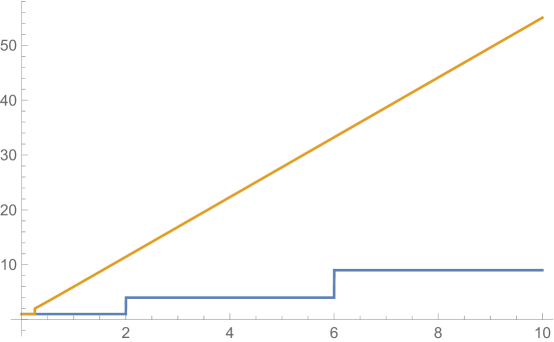
Figure 1: The estimate of the counting function for ${\mathbb{S}}^{2}$. The piecewise constant function is $N(x)$ and the other function is given by Theorem 3.1 and Remark 3.5.

Example 7.3 (Hyperbolic spaces).

Because the heat kernel is the Laplace transform of the spectral measure—see (5.1)—the spectral function for a noncompact symmetric space $X$ can sometimes be determined if one has an exact expression for its heat kernel. Note that if $X$ is a rank-one symmetric space, then $e_{\lambda}(x,y)$ depends only on the distance $r:=r(x,y)$ between $x$ and $y$.

For example, if $d\geq 3$ is odd, then, according to [1], the heat kernel for real hyperbolic space ${\mathbb{H}}^{d}({\mathbb{R}})$ is

(7.2) $$p_{t}(x,y)\leavevmode\nobreak\ =\leavevmode\nobreak\ \frac{\sqrt{\pi}}{(2\pi)^{\frac{d+1}{2}}}\cdot\frac{\exp\left(-b_{d}\cdot t\right)}{\sqrt{t}}\cdot\left(\frac{-1}{\sinh(r)}\partial_{r}\right)^{\frac{d-1}{2}}\exp\left(\frac{-r^{2}}{4t}\right)\,,$$

where $b_{d}:=(d-1)^{2}/4$ is the bottom of the spectrum. We claim that if $r=\operatorname{{dist}}(x,y)>0$, then

(7.3) $$e_{\lambda}(x,y)\leavevmode\nobreak\ =\leavevmode\nobreak\ \begin{cases}\displaystyle\frac{2}{(2\pi)^{\frac{d+1}{2}}}\left(\frac{-1}{\sinh(r)}\partial_{r}\right)^{\frac{d-1}{2}}\frac{\sin(r\cdot\sqrt{\lambda-b_{d}})}{r}&\text{if }\lambda\geq b_{d},\\[12.91663pt] 0&\text{otherwise}.\end{cases}$$

Indeed, by taking the Laplace transform of $de_{\lambda}$, making the change of variable $\lambda=\nu+b_{d}$, and applying the identity

$$\int_{0}^{\infty}e^{-\nu\cdot t}\,d_{\nu}\left(\frac{\sin(r\sqrt{\nu})}{r}\right)\leavevmode\nobreak\ =\leavevmode\nobreak\ \frac{\sqrt{\pi}}{2\sqrt{t}}\cdot\exp\left(\frac{-r^{2}}{4t}\right)\,,$$

we obtain (7.2) from (7.3). Thus, (7.3) follows from the fact that the Laplace transform is injective on bounded functions.

One obtains an explicit expression for $N_{x}(\lambda)$ from (7.3) by differentiating and taking the limit as $r$ tends to zero. For example, the values of $N_{x}(\lambda)$ for $d=3,5,7$ and $\lambda\geq b_{d}$ are

$$\frac{(\lambda-1)^{3/2}}{6\pi^{2}}\,,\ \frac{(3(\lambda-4)+5)(\lambda-4)^{3/2}}{180\pi^{3}}\,,\ \frac{\left(3(\lambda-9)^{2}+21(\lambda-9)+28\right)(\lambda-9)^{3/2}}{2520\pi^{4}}\,.$$

For even-dimensional real hyperbolic spaces, a similar analysis using the explicit formula for the heat kernel [1] gives

$$e_{\lambda}(x,y)\leavevmode\nobreak\ =\leavevmode\nobreak\ \frac{2\sqrt{2}}{(2\pi)^{(d+2)/2}}\int_{r}^{\infty}\frac{\sinh s}{\sqrt{\cosh s-\cosh r}}\cdot\left(\frac{-1}{\sinh s}\partial_{s}\right)^{\frac{d}{2}}\frac{\sin(s\cdot\sqrt{\lambda-b_{d}})}{s}\,ds\,.$$

It is convenient to write

$$\frac{\sin(s\cdot\sqrt{\lambda-b_{d}})}{s}=\int_{0}^{\sqrt{\lambda-b_{d}}}\cos(s\cdot a)\,da$$

in the preceding integral. Using Fubini’s theorem, we then obtain for $d=2$ and $\lambda\geq 1/4$ that

$$N_{x}(\lambda)\leavevmode\nobreak\ =\leavevmode\nobreak\ \int_{0}^{\sqrt{\lambda-1/4}}\frac{a\tanh(\pi a)}{2\pi}\,da\,;$$

when $d=4$, we obtain for $\lambda\geq 9/4$ that

$$N_{x}(\lambda)\leavevmode\nobreak\ =\leavevmode\nobreak\ \int_{0}^{\sqrt{\lambda-9/4}}\frac{\left(4a^{3}+a\right)\tanh(\pi a)}{32\pi^{2}}\,da\,;$$

and when $d=6$, we obtain for $\lambda\geq 25/4$ that

$$N_{x}(\lambda)\leavevmode\nobreak\ =\leavevmode\nobreak\ \int_{0}^{\sqrt{\lambda-25/4}}\frac{\left(16a^{5}+40a^{3}+9a\right)\tanh(\pi a)}{1024\pi^{3}}\,da\,.$$

The volume of the ball of radius $r$ in ${\mathbb{H}}^{d}({\mathbb{R}})$ is given by

$$V(r)\leavevmode\nobreak\ =\leavevmode\nobreak\ \operatorname{\mathsf{vol}}({\mathbb{S}}^{d-1})\int_{0}^{r}(\sinh x)^{d-1}\,dx\,.$$

In particular, if $d=2$, then Theorem 4.9 yields the estimate

$$N_{x}(\lambda)\leavevmode\nobreak\ \leq\leavevmode\nobreak\ \frac{4\lambda+1}{2\pi\bigl{(}4\lambda\sinh^{2}\bigl{(}\frac{\pi}{4\sqrt{\lambda}}\bigr{)}-1\bigr{)}}\,.$$

See Figure 2.

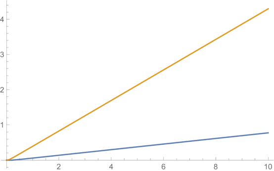
Figure 2: The lower curve is $N_{x}$ for ${\mathbb{H}}^{2}({\mathbb{R}})$ and the upper curve is the estimate given by Theorem 4.9.

Because we could not find the spectral functions for complex hyperbolic spaces in the literature, we give them here as well. For $M={\mathbb{H}}^{d}({\mathbb{C}})$ with $d\geq 2$, using the Laplace transform and the formula for the heat kernel [1], we obtain that for $\lambda\geq d^{2}$ and $\operatorname{{dist}}(x,y)=r$,

$$e_{\lambda}(x,y)\leavevmode\nobreak\ =\leavevmode\nobreak\ \frac{4\sqrt{2}}{(2\pi)^{d+1}}\int_{r}^{\infty}\frac{\sinh s}{\sqrt{\cosh 2s-\cosh 2r}}\cdot\left(\frac{-1}{\sinh s}\partial_{s}\right)^{d}\frac{\sin(s\cdot\sqrt{\lambda-d^{2}})}{s}\,ds\,.$$

For $d=2$, this yields for $\lambda\geq 4$ that

$$N_{x}(\lambda)\leavevmode\nobreak\ =\leavevmode\nobreak\ \int_{0}^{\sqrt{\lambda-4}}\frac{a^{3}\coth(\pi a/2)}{8\pi^{2}}\,da\,;$$

for $d=3$, this yields for $\lambda\geq 9$ that

$$N_{x}(\lambda)\leavevmode\nobreak\ =\leavevmode\nobreak\ \int_{0}^{\sqrt{\lambda-9}}\frac{a(a^{2}+1)^{2}\tanh(\pi a/2)}{64\pi^{3}}\,da\,;$$

and for $d=4$, this yields for $\lambda\geq 16$ that

$$N_{x}(\lambda)\leavevmode\nobreak\ =\leavevmode\nobreak\ \int_{0}^{\sqrt{\lambda-16}}\frac{a^{3}(a^{2}+4)^{2}\coth(\pi a/2)}{768\pi^{4}}\,da\,.$$

Appendix A Integral kernels and the functional calculus

It is known that the spectral projection $E_{\lambda}$ has a smooth kernel in the case of noncompact manifolds; see, for example, [14]. However, we found it difficult to find a complete proof in the literature, and so we provide a proof here as a courtesy to the reader. We also prove some other facts about the kernel that we use.

The proof of smoothness relies on the standard theory of elliptic partial differential equations. If $\Delta^{k}u=v$, then since $\Delta$ is self-adjoint, we have, for each compactly supported smooth function $\psi$,

(A.1) $$\langle\Delta^{k}\psi,u\rangle\leavevmode\nobreak\ =\leavevmode\nobreak\ \langle\psi,v\rangle\,.$$

That is, if we regard $u$ and $v$ as distributions, then $L^{k}u=v$, where $L$ is the Laplacian acting on distributions. Here, $L^{k}$ is an elliptic differential operator of order $2k$. Our assumption $\Delta^{k}u=v$ involves a function class $u\in{\mathcal{H}}=L^{2}(M,\mu)$, but we will need to show that there is a function in the class of $u$ that has continuous derivatives. Thus, we explain next a few facts about Sobolev spaces that we need, which is a theory of distributions.

Let $U\subset M$ be a precompact open set whose closure lies in an open set diffeomorphic to ${\mathbb{R}}^{d}$. A function (class) $v\in{\mathcal{H}}$, regarded as a distribution restricted to $U$, lies in the Sobolev space $H^{0}(U)$. If $u$ is a distribution with $L^{k}u=v$, then the standard theory of elliptic equations implies that $u$ lies in the Sobolev space $H^{2k}(U)$. Moreover, there exists a constant $C=C(L,U,k)$ so that

(A.2) $$\|u\|_{H^{2k}(U)}\leavevmode\nobreak\ \leq\leavevmode\nobreak\ C\cdot\bigl{(}\|v\|+\|u\|\bigr{)}\,.$$

Choose coordinates $(x_{1},x_{2},\ldots,x_{d})$ on $U$, and for each multi-index $\alpha\in{\mathbb{N}}^{d}$, let $\partial^{\alpha}$ denote the mixed partial derivative $\partial^{\alpha_{1}}_{x_{1}}\cdots\partial^{\alpha_{d}}_{x_{d}}$. For each $u\colon U\rightarrow{\mathbb{R}}$ such that $\partial^{\alpha}u$ is continuous and bounded for each $\alpha$ with $|\alpha|:=\sum\alpha_{i}\leq j$, define

(A.3) $$\|u\|_{C^{j}(U)}\leavevmode\nobreak\ =\leavevmode\nobreak\ \sup_{U}\,|u|_{C^{j}}\,,$$

where

$$|u|_{C^{j}}(x)\leavevmode\nobreak\ :=\leavevmode\nobreak\ \sup_{|\alpha|\leq j}\,\left|\partial^{\alpha}u(x)\right|\,.$$

The Sobolev embedding theorem provides constants $C^{\prime}=C^{\prime}(U,k,j)$ so that if $u\in H^{2k}(U)$ and $2k>d/2+j+1$, then the distribution $u$ is represented by a function with a continuous $j^{{\rm th}}$ derivative, which we also denote by $u$, and

$$\|u\|_{C^{j}(U)}\leavevmode\nobreak\ \leq\leavevmode\nobreak\ C^{\prime}\cdot\|u\|_{H^{2k}(U)}\,.$$

Recall that $E$ denotes the spectral resolution of $\Delta$.

Theorem A.1.

Let $a\colon[0,\infty)\to{\mathbb{R}}$ be a nonnegative Borel function such that for each nonnegative integer $k$, the map $\nu\mapsto a(\nu)\cdot\nu^{k}$ is bounded on $[0,\infty)$. Then the operator $a(\Delta)$ defined by

$$a(\Delta)\leavevmode\nobreak\ =\leavevmode\nobreak\ \int_{0}^{\infty}a(\nu)\leavevmode\nobreak\ dE_{\nu}$$

maps each element of ${\mathcal{H}}$ to a smooth function, and $a(\Delta)$ has a smooth, symmetric, real-valued integral kernel.

Proof.

The hypothesis implies that, for each $k$, the operator $\Delta^{k}\circ\sqrt{a}(\Delta)$ maps ${\mathcal{H}}$ to ${\mathcal{H}}$. Given $w\in{\mathcal{H}}$, let $u:=\sqrt{a}(\Delta)(w)$ and $v:=\Delta^{k}u$. Regarding $u$ and $v$ as distributions, we have $L^{k}u=v$. Given $x\in M$, let $U\ni x$ be a precompact open set whose closure lies in an open set diffeomorphic to ${\mathbb{R}}^{d}$. By the discussion above, the distribution $u$ lies in $H^{2k}(U)$ and (A.2) holds, and if we choose $2k>d/2+j+1$, then

$$|u|_{C^{j}}(x)\leavevmode\nobreak\ \leq\leavevmode\nobreak\ C^{\prime}\cdot\|u\|_{H^{2k}(U)}\leavevmode\nobreak\ \leq\leavevmode\nobreak\ C^{\prime}\cdot C\cdot\bigl{(}\|v\|+\|u\|\bigr{)}\,,$$

and hence, since $\Delta^{k}\circ\sqrt{a}(\Delta)$ is a bounded linear operator, we have

(A.4) $$\left|(\sqrt{a}(\Delta))w\right|_{C^{j}}(x)\leavevmode\nobreak\ \leq\leavevmode\nobreak\ C^{\prime}\cdot C\cdot\left(\|\Delta^{k}\circ\sqrt{a}(\Delta)w\|\leavevmode\nobreak\ +\|w\|\right)\leavevmode\nobreak\ \leq\leavevmode\nobreak\ C^{*}\cdot\|w\|$$

for some constant $C^{*}=C^{*}(U,j,k)$. In particular, $\sqrt{a}(\Delta)w$ is smooth.

For each $x$, define the linear functional $f_{x}\colon{\mathcal{H}}\to{\mathbb{R}}$ by $f_{x}(w):=(\sqrt{a}(\Delta)w)(x)$. From (A.4) with $j=0$, we see that the functional $f_{x}$ is bounded, and therefore there exists $k_{x}\in{\mathcal{H}}$ so that for each $w\in{\mathcal{H}}$ we have $\langle w,k_{x}\rangle=f_{x}(w)=(\sqrt{a}(\Delta)w)(x)$.

We claim that $k_{x}(y)=k_{y}(x)$ for almost every $(x,y)\in M\times M$. Indeed, since $\sqrt{a}(\Delta)$ is self-adjoint, $k_{x}$ is real valued and $\langle\sqrt{a}(\Delta)w_{-},\overline{w_{+}}\rangle=\langle w_{-},\sqrt{a}(\Delta)\overline{w_{+}}\rangle$ for each $w_{-},w_{+}\in{\mathcal{H}}$. Hence

$$\int_{M\times M}w_{-}(x)\cdot w_{+}(y)\cdot k_{x}(y)\,(d\mu\times d\mu)(x,y)\\ =\int_{M\times M}w_{+}(y)\cdot w_{-}(x)\cdot k_{x}(y)\,(d\mu\times d\mu)(x,y)\,.$$

By switching the roles of $x$ and $y$ in the latter integral and subtracting, we find that

$$\int_{M\times M}\psi(x,y)\cdot\bigl{(}k_{x}(y)-k_{y}(x)\bigr{)}\,(d\mu\times d\mu)(x,y)\leavevmode\nobreak\ =\leavevmode\nobreak\ 0\,,$$

where $\psi(x,y):=w_{-}(x)\cdot w_{+}(y)$. Since such $\psi$ span a dense subspace of $L^{2}(M\times M,\mu\times\mu)$, the claim follows.

Define $K\colon M\times M\to{\mathbb{R}}$ by

$$K(x,y)\leavevmode\nobreak\ :=\leavevmode\nobreak\ \int_{M}k_{x}(z)\cdot k_{y}(z)\,d\mu(z)\,.$$

Using the symmetry $k_{y}(z)=k_{z}(y)$ $\>\mu\times\mu$-a.e. and the fact that $\sqrt{a}\cdot\sqrt{a}=a$, one finds that $K$ is an integral kernel for $a(\Delta)$. To finish the proof of the theorem, it suffices to show that $K$ is a smooth function.

Let $\alpha\in{\mathbb{N}}^{d}$ be a multi-index. Let $U_{x}$ and $U_{y}$ be neighborhoods of $x,y\in M$. Using (A.4), we find that the map $w\mapsto\partial^{\alpha}_{x}(\sqrt{a}(\Delta)w)(x)$ is a bounded linear functional on ${\mathcal{H}}$. Hence there exists $k_{x}^{\alpha}\in{\mathcal{H}}$ so that

$$\langle k_{x}^{\alpha},w\rangle\leavevmode\nobreak\ =\leavevmode\nobreak\ \partial^{\alpha}_{x}(\sqrt{a}(\Delta)w)(x)\leavevmode\nobreak\ =\leavevmode\nobreak\ \partial_{x}^{\alpha}\langle k_{x},w\rangle\,.$$

Thus, we have

$$\partial^{\beta}_{y}\partial^{\alpha}_{x}K(x,y)\leavevmode\nobreak\ =\leavevmode\nobreak\ \partial^{\beta}_{y}\partial_{x}^{\alpha}\langle k_{x},k_{y}\rangle\leavevmode\nobreak\ =\leavevmode\nobreak\ \partial^{\beta}_{y}\langle k_{x}^{\alpha},k_{y}\rangle\leavevmode\nobreak\ =\leavevmode\nobreak\ \langle k_{x}^{\alpha},k_{y}^{\beta}\rangle\,.$$

In particular, $K$ is smooth. ∎

Let $e_{\lambda}(x,y)$ denote the kernel corresponding to the spectral projection $E_{\lambda}={\bf 1}_{[0,\lambda]}(\Delta)$. Write $F_{x}^{\lambda}(y):=e_{\lambda}(x,y)$, so that $F_{x}^{\lambda}$ is an element of ${\mathcal{H}}$ with norm 1. For continuous $a\colon[0,\infty)\to{\mathbb{R}}$ with support in $[0,\lambda]$ and all $\nu\geq\lambda$, we have $\langle a(\Delta)F_{x}^{\nu},F_{y}^{\nu}\rangle=\langle a(\Delta)F_{x}^{\lambda},F_{y}^{\lambda}\rangle$, with $|\langle a(\Delta)F_{x}^{\lambda},F_{y}^{\lambda}\rangle|\leq\|a\|_{\infty}$ by the Cauchy–Schwarz inequality. Therefore, $\lambda\mapsto e_{\lambda}(x,y)$ is a function of bounded variation and defines a bounded measure on the real line that satisfies

$$\int_{0}^{\infty}a(\nu)\,de_{\nu}(x,y)\leavevmode\nobreak\ =\leavevmode\nobreak\ \langle a(\Delta)F_{x}^{\lambda},F_{y}^{\lambda}\rangle$$

whenever $a$ is a bounded Borel function with support in $[0,\lambda]$.

Proposition A.2.

Let $a\colon[0,\infty)\to{\mathbb{R}}$ be a nonnegative Borel function such that for each nonnegative integer $k$, the map $\nu\mapsto a(\nu)\cdot\nu^{k}$ is bounded on $[0,\infty)$. Then the kernel of $a(\Delta)$ is

$$(x,y)\mapsto A_{x}(y)\leavevmode\nobreak\ :=\leavevmode\nobreak\ \int_{0}^{\infty}a(\lambda)\,de_{\lambda}(x,y)\,.$$

Proof.

Let $K$ be the kernel given by Theorem A.1 and $K_{x}(y):=K(x,y)$. Then for $x\in M$ and $u\in{\mathcal{H}}_{\nu}$, we have $a(\Delta)u\in{\mathcal{H}}_{\nu}$ and

$$\langle u,K_{x}\rangle \leavevmode\nobreak\ =\leavevmode\nobreak\ a(\Delta)u(x)\leavevmode\nobreak\ =\leavevmode\nobreak\ \Bigl{\langle}\int_{0}^{\nu}a(\lambda)\,dE_{\lambda}u,F_{x}^{\nu}\Bigr{\rangle}\leavevmode\nobreak\ =\leavevmode\nobreak\ \int_{0}^{\nu}a(\lambda)\,d\langle E_{\lambda}u,F_{x}^{\nu}\rangle$$

$$\leavevmode\nobreak\ =\leavevmode\nobreak\ \int_{0}^{\nu}a(\lambda)\,d\langle u,F_{x}^{\lambda}\rangle\leavevmode\nobreak\ =\leavevmode\nobreak\ \Bigl{\langle}u,\int_{0}^{\nu}a(\lambda)\,dF_{x}^{\lambda}\Bigr{\rangle}\leavevmode\nobreak\ =\leavevmode\nobreak\ \langle u,A_{x}\rangle\,.$$

Since $\langle u,K_{x}\rangle=\langle u,A_{x}\rangle$ for such $u$ and $\bigcup_{\nu}{\mathcal{H}}_{\nu}$ is dense in ${\mathcal{H}}$, we obtain that $K_{x}=A_{x}$, as desired. ∎

Proposition A.3.

Let $K$ be the kernel of $a(\Delta)$ constructed in Theorem A.1. For each $x$, the function $y\mapsto|\nabla_{x}K(x,y)|^{2}$ is integrable.

Proof.

Choose normal coordinates $(x_{1},\ldots,x_{d})$ about the point $x$, and let $\partial_{i}$ be the associated coordinate vector fields. By (A.4), for each $i$, there exists $k_{x}^{i}\in{\mathcal{H}}$ so that $\langle k_{x}^{i},u\rangle=\partial_{i}\langle k_{x},u\rangle$ for each $u\in{\mathcal{H}}$. Thus,

$$|\nabla_{x}K(x,y)|^{2}\leavevmode\nobreak\ =\leavevmode\nobreak\ \sum_{i}|\partial_{i}\langle k_{x},k_{y}\rangle|^{2}\leavevmode\nobreak\ =\leavevmode\nobreak\ \sum_{i}\langle k_{x}^{i},k_{y}\rangle^{2}.$$

On the other hand, the defining property of $k_{y}$ yields $\langle k_{x}^{i},k_{y}\rangle=(\sqrt{a}(\Delta)k_{x}^{i})(y)$. Since $\sqrt{a}(\Delta)$ maps ${\mathcal{H}}$ to ${\mathcal{H}}$, the function $y\mapsto(\sqrt{a}(\Delta)k_{x}^{i})(y)$ is square-integrable. The claim follows from summing over $i$. ∎

The work of C.J. is partially supported by a Simons collaboration grant. The work of R.L. is partially supported by the National Science Foundation under grants DMS-1007244 and DMS-1612363.

References

- [1] \RMIauthorAnker, J.-P. and Ostellari, P. \RMIpaperThe heat kernel on noncompact symmetric spaces In \RMIbookLie groups and Symmetric Spaces, 27–46 Amer. Math. Soc. Transl. Ser. 2, 210, Amer. Math. Soc., Providence, RI, 2003.
- [2] \RMIauthorBerger, M. \RMIbookA Panoramic View of Riemannian Geometry Springer-Verlag, Berlin, 2003.
- [3] \RMIauthorBers, L., John, F., and Schechter, M. \RMIbookPartial Differential Equations With supplements by Lars Gårding and A. N. Milgram. With a preface by A. S. Householder. Reprint of the 1964 original. Lectures in Applied Mathematics, 3A. American Mathematical Society, Providence, RI, 1979.
- [4] \RMIauthorBerti, M. and Procesi, M. \RMIpaperNonlinear wave and Schrödinger equations on compact Lie groups and homogeneous spaces \RMIjournal Duke Math. J. 159 (2011), no. 3, 479–538.
- [5] \RMIauthorDavies, E.B. \RMIbook Heat Kernels and Spectral Theory Cambridge Tracts in Mathematics, 92. Cambridge University Press, Cambridge, 1990.
- [6] \RMIauthorCheeger, J. and Ebin, D. \RMIbookComparison Theorems in Riemannian Geometry Revised reprint of the 1975 original. AMS Chelsea Publishing, Providence, RI, 2008.
- [7] \RMIauthor Efremov, D.V. and Shubin, M.A. \RMIpaperSpectrum distribution function and variational principle for automorphic operators on hyperbolic space In \RMIbookSéminaire sur les Équations aux Dérivées Partielles, 1988–1989 Exp. No. VIII, 19. École Polytech., Palaiseau, 1989.
- [8] \RMIauthorGaffney, M.P. \RMIpaperHilbert space methods in the theory of harmonic integrals \RMIjournalTrans. Amer. Math. Soc. 78, (1955), 426–444.
- [9] \RMIauthorGallot, S., Hulin, D., and Lafontaine, J. \RMIbookRiemannian Geometry Third edition. Universitext. Springer-Verlag, Berlin, 2004
- [10] \RMIauthorGrebenkov, D.S. and Nguyen, B.-T. \RMIbookGeometrical structure of Laplacian eigenfunctions \RMIjournalSIAM Rev. 55 (2013), no. 4, 601–667.
- [11] \RMIauthorGromov, M. \RMIbookMetric Structures for Riemannian and Non-Riemannian Spaces Progress in Mathematics, 152. Birkhäuser Boston, Inc., Boston, MA, 1999.
- [12] \RMIauthorGünther, P. \RMIpaperEinige Sätze über das Volumenelement eines Riemannschen Raumes Publ. Math. Debrecen 7 (1960), 78–93.
- [13] \RMIauthorHelgason, S. \RMIbookDifferential Geometry and Symmetric Spaces. Pure and Applied Mathematics, Vol. XII. Academic Press, New York-London, 1962.
- [14] \RMIauthorHörmander, L. \RMIpaperOn the Riesz means of spectral functions and eigenfunction expansions for elliptic differential operators. In \RMIbookSome Recent Advances in the Basic Sciences, 155–202 Vol. 2, Belfer Graduate School of Science, Yeshiva Univ., New York, 1966.
- [15] \RMIauthorHörmander, L. \RMIpaperThe spectral function of an elliptic operator \RMIjournalActa Math. 121 (1968), 193–218.
- [16] \RMIauthorLax, P.D. and Phillips, R.S. \RMIpaperThe asymptotic distribution of lattice points in Euclidean and non-Euclidean spaces \RMIjournalJ. Funct. Anal. 46 (1982), no. 3, 280–350.
- [17] \RMIauthorLi, P. \RMIpaperEigenvalue estimates on homogeneous manifolds \RMIjournalComment. Math. Helv. 55 (1980), no. 3, 347–363.
- [18] \RMIauthorLi, P. \RMIbookGeometric Analysis Cambridge Studies in Advanced Mathematics, 134. Cambridge University Press, Cambridge, 2012.
- [19] \RMIauthorLi, P. and Yau, S.-T. \RMIpaperEstimates of eigenvalues of a compact Riemannian manifold In \RMIbookGeometry of the Laplace Operator, 205–239 Proc. Sympos. Pure Math., XXXVI, Amer. Math. Soc., Providence, RI, 1980.
- [20] \RMIauthorLyons, R. and Oveis Gharan, S. \RMIpaperSharp bounds on random walk eigenvalues via spectral embedding \RMIjournalIMRN, rnx082, to appear.
- [21] \RMIauthorNatalini P. and Palumbo, B. \RMIpaperInequalities for the incomplete gamma function \RMIjournalMath. Inequal. Appl. 3 (2000), no. 1, 69–77.
- [22] \RMIauthorPittet, Ch. \RMIpaperThe isoperimetric profile of homogeneous Riemannian manifolds \RMIjournalJ. Differential Geom. 54 (2000) no. 2, 255–302.
- [23] \RMIauthorPortegies, J.W. \RMIpaperEmbeddings of Riemannian manifolds with heat kernels and eigenfunctions \RMIjournalCommun. Pure Appl. Math. 69 (2016), no. 3, 478–518.
- [24] \RMIauthorReed, M. and Simon, B. \RMIbookMethods of Modern Mathematical Physics. II. Fourier Analysis, Self-adjointness. Academic Press [Harcourt Brace Jovanovich, Publishers], New York-London, 1975.
- [25] \RMIauthorSolomon, B. \RMIpaperThe harmonic analysis of cubic isoparametric minimal hypersurfaces. I. Dimensions 3 and 6 \RMIjournalAmer. J. Math. 112 (1990), no. 2, 157–203.
- [26] \RMIauthorSolomon, B. \RMIpaperThe harmonic analysis of cubic isoparametric minimal hypersurfaces. II. Dimensions 12 and 24 \RMIjournalAmer. J. Math. 112 (1990), no. 2, 205–241.
- [27] \RMIauthorStrichartz, R.S. \RMIpaperAnalysis of the Laplacian on the complete Riemannian manifold \RMIjournalJ. Funct. Anal. 52 (1983), no. 1, 48–79.
- [28] \RMIauthorVaradarajan, V.S. \RMIbookLie Groups, Lie Algebras, and Their Representations Graduate Texts in Mathematics, 102. Springer-Verlag, New York, 1984.
- [29] \RMIauthorVaropoulos, N. Th. \RMIpaperAnalysis on Lie groups \RMIjournalRev. Mat. Iberoamericana 12 (1996), no. 3, 791–917.