Computing top-$k$ Closeness Centrality Faster in Unweighted Graphs

Abstract

Given a connected graph $G=(V,E)$, the closeness centrality of a vertex $v$ is defined as $\frac{n-1}{\sum_{w\in V}d(v,w)}$. This measure is widely used in the analysis of real-world complex networks, and the problem of selecting the $k$ most central vertices has been deeply analysed in the last decade. However, this problem is computationally not easy, especially for large networks: in the first part of the paper, we prove that it is not solvable in time $\mathcal{O}(|E|^{2-\epsilon})$ on directed graphs, for any constant $\epsilon>0$, under reasonable complexity assumptions. Furthermore, we propose a new algorithm for selecting the $k$ most central nodes in a graph: we experimentally show that this algorithm improves significantly both the textbook algorithm, which is based on computing the distance between all pairs of vertices, and the state of the art. For example, we are able to compute the top $k$ nodes in few dozens of seconds in real-world networks with millions of nodes and edges. Finally, as a case study, we compute the $10$ most central actors in the IMDB collaboration network, where two actors are linked if they played together in a movie, and in the Wikipedia citation network, which contains a directed edge from a page $p$ to a page $q$ if $p$ contains a link to $q$.

<ccs2012> <concept> <concept_id>10003120.10003130.10003134.10003293</concept_id> <concept_desc>Human-centered computing Social network analysis</concept_desc> <concept_significance>500</concept_significance> </concept> <concept> <concept_id>10002950.10003624.10003633.10010917</concept_id> <concept_desc>Mathematics of computing Graph algorithms</concept_desc> <concept_significance>500</concept_significance> </concept> </ccs2012>

[500]Human-centered computing Social network analysis [500]Mathematics of computing Graph algorithms

1 Introduction

The problem of identifying the most central nodes in a network is a fundamental question that has been asked many times in a plethora of research areas, such as biology, computer science, sociology, and psychology. Because of the importance of this question, dozens of centrality measures have been introduced in the literature (for a recent survey, see [Boldi and Vigna (2014)]). Among these measures, closeness centrality is certainly one of the oldest and of the most widely used [Bavelas (1950)]: almost all books dealing with network analysis discuss it (for example, [Newman (2010)]), and almost all existing network analysis libraries implement algorithms to compute it.

In a connected graph, the closeness centrality of a node $v$ is defined as $c(v)=\frac{n-1}{\sum_{w\in V}d(v,w)}$. The idea behind this definition is that a central node should be very efficient in spreading information to all other nodes: for this reason, a node is central if the average number of links needed to reach another node is small. If the graph is not (strongly) connected, researchers have proposed various ways to extend this definition: for the sake of simplicity, we focus on Lin’s index, because it coincides with closeness centrality in the connected case and because it is quite established in the literature [Lin (1976), Wasserman and Faust (1994), Boldi and Vigna (2013), Boldi and Vigna (2014), Olsen et al. (2014)]. However, our algorithms can be adapted very easily to compute other possible generalizations, such as harmonic centrality [Marchiori and Latora (2000)] and exponential centrality [Wang and Tang (2014)] (see Sect. 2 for more details).

In order to compute the $k$ vertices with largest closeness, the textbook algorithm computes $c(v)$ for each $v$ and returns the $k$ largest found values. The main bottleneck of this approach is the computation of $d(v,w)$ for each pair of vertices $v$ and $w$ (that is, solving the All Pairs Shortest Paths or APSP problem). This can be done in two ways: either by using fast matrix multiplication, in time $\mathcal{O}(n^{2.373}\log n)$ [Zwick (2002), Williams (2012)], or by performing a breadth-first search (in short, BFS) from each vertex $v\in V$, in time $\mathcal{O}(mn)$, where $n=|V|$ and $m=|E|$. Usually, the BFS approach is preferred because the other approach contains big constants hidden in the $\mathcal{O}$ notation, and because real-world networks are usually sparse, that is, $m$ is not much bigger than $n$. However, also this approach is too time-consuming if the input graph is very big (with millions of nodes and hundreds of millions of edges).

Our first result proves that, in the worst case, the BFS-based approach cannot be improved, under reasonable complexity assumptions. Indeed, we construct a reduction from the problem of computing the most central vertex (the case $k=1$) to the Orthogonal Vector problem [Abboud et al. (2016)]. This reduction implies that we cannot compute the most central vertex in $\mathcal{O}(m^{2-\epsilon})$ for any $\epsilon>0$, unless the Orthogonal Vector conjecture [Abboud et al. (2016)] is false. Note that the Orthogonal Vector conjecture is implied by the well-known Strong Exponential Time Hypothesis (SETH, [Impagliazzo et al. (2001)]), and hence all our results hold also if we assume SETH. This hypothesis is heavily used in the context of polynomial-time reductions, and, informally, it says that the Satisfiability problem is not solvable in time $\mathcal{O}((2-\epsilon)^{N})$ for any $\epsilon>0$, where $N$ is the number of variables. Our result still holds if we assume the input graph to be sparse, that is, if we assume that $m=\mathcal{O}(n)$ (the general non-sparse case follows immediately; of course, if the input graph is not sparse, then the BFS-based approach can be improved using fast matrix multiplication). The proof is provided in Sect. 3.

Knowing that the BFS-based algorithm cannot be improved in the worst case, in the second part of the paper we provide a new exact algorithm that performs much better on real-world networks, making it possible to compute the $k$ most central vertices in networks with millions of nodes and hundreds of millions of edges. The new approach combines the BFS-based algorithm with a pruning technique: during the algorithm, we compute and update upper bounds on the closeness of all the nodes, and we exclude a node $v$ from the computation as soon as its upper bound is “small enough”, that is, we are sure that $v$ does not belong to the top $k$ nodes. We propose two different strategies to set the initial bounds, and two different strategies to update the bounds during the computation: this means that our algorithm comes in four different variations. The experimental results show that different variations perform well on different kinds of networks, and the best variation of our algorithm drastically outperforms both a probabilistic approach [Okamoto et al. (2008)], and the best exact algorithm available until now [Olsen et al. (2014)]. We have computed for the first time the $10$ most central nodes in networks with millions of nodes and hundreds of millions of edges, and do so in very little time. A significant example is the wiki-Talk network, which was also used in [Sariyüce et al. (2013)], where the authors propose an algorithm to update closeness centralities after edge additions or deletions. Our performance is about $30\,000$ times better than the performance of the textbook algorithm: if only the most central node is needed, we can recompute it from scratch more than $150$ times faster than the geometric average update time in [Sariyüce et al. (2013)]. Moreover, our approach is not only very efficient, but it is also very easy to code, making it a very good candidate to be implemented in existing graph libraries. We provide an implementation of it in NetworKit [Staudt et al. (2014)] and of one of its variations in Sagemath [Csárdi and Nepusz (2006)]. We sketch the main ideas of the algorithm in Sect. 4, and we provide all details in Sect. 5-8. We experimentally evaluate the efficiency of the new algorithm in Sect. 9.

Also, our approach can be easily extended to any centrality measure in the form $c(v)=\sum_{w\neq v}f(d(v,w))$, where $f$ is a decreasing function. Apart from Lin’s index, almost all the approaches that try to generalize closeness centrality to disconnected graphs fall under this category. The most popular among these measures is harmonic centrality [Marchiori and Latora (2000)], defined as $h(v)=\sum_{w\neq v}\frac{1}{d(v,w)}$. For the sake of completeness, in Sect. 9 we show that our algorithm performs well also for this measure.

In the last part of the paper (Sect. 10, 11), we consider two case studies: the actor collaboration network ($1\,797\,446$ vertices, $72\,880\,156$ edges) and the Wikipedia citation network ($4\,229\,697$ vertices, $102\,165\,832$ edges). In the actor collaboration network, we analyze the evolution of the $10$ most central vertices, considering snapshots taken every 5 years between 1940 and 2014. The computation was performed in little more than $45$ minutes. In the Wikipedia case study, we consider both the standard citation network, that contains a directed edge $(p,q)$ if $p$ contains a link to $q$, and the reversed network, that contains a directed edge $(p,q)$ if $q$ contains a link to $p$. For most of these graphs, we are able to compute the $10$ most central pages in a few minutes, making them available for further analyses.

1.1 Related Work

Closeness is a “traditional” definition of centrality, and consequently it was not “designed with scalability in mind”, as stated in [Kang et al. (2011)]. Also in [Chen et al. (2012)], it is said that closeness centrality can “identify influential nodes”, but it is “incapable to be applied in large-scale networks due to the computational complexity”. The simplest solution considered was to define different measures that might be related to closeness centrality [Kang et al. (2011)].

Hardness results

A different line of research has tried to develop more efficient algorithms, or lower bounds for the complexity of this problem. In particular, in [Borassi et al. (2015)] it is proved that finding the least closeness-central vertex is not subquadratic-time solvable, unless SETH is false. In the same line, it is proved in [Abboud et al. (2016)] that finding the most central vertex is not solvable in $\mathcal{O}(m^{2-\epsilon})$, assuming the Hitting Set conjecture. This conjecture is very recent, and there are not strong evidences that it holds, apart from its similarity to the Orthogonal Vector conjecture. Conversely, the Orthogonal Vector conjecture is more established: it is implied both by the Hitting Set conjecture [Abboud et al. (2016)], and by SETH [Williams (2005)], a widely used assumption in the context of polynomial-time reductions [Impagliazzo et al. (2001), Williams (2005), Williams and Williams (2010), Pǎtraşcu and Williams (2010), Roditty and Williams (2013), Abboud et al. (2014), Abboud and Williams (2014), Abboud et al. (2015), Borassi et al. (2015), Abboud et al. (2016), Borassi (2016)]. Similar hardness results were also proved in the dense weighted context [Abboud et al. (2015)], by linking the complexity of centrality measures to the complexity of computing the All Pairs Shortest Paths.

Approximation algorithms

In order to deal with the above hardness results, it is possible to design approximation algorithms: the simplest approach samples the distance between a node $v$ and $l$ other nodes $w$, and returns the average of all values $d(v,w)$ found [Eppstein and Wang (2004)]. The time complexity is $\mathcal{O}(lm)$, to obtain an approximation $\tilde{c}(v)$ of the centrality of each node $v$ such that $\mathbb{P}\left(\left|\frac{1}{\tilde{c}(v)}-\frac{1}{c(v)}\right|\geq\epsilon D\right)\leq 2e^{-\Omega\left(l\epsilon^{2}\right)}$, where $D$ is the diameter of the graph (the diameter is the maximum distance between any two connected nodes). A more refined approximation algorithm is provided in [Cohen et al. (2014)], which combines the sampling approach with a $3$-approximation algorithm: this algorithm has running time $\mathcal{O}(lm)$, and it provides an estimate $\tilde{c}(v)$ of the centrality of each node $v$ such that $\mathbb{P}\left(\left|\frac{1}{\tilde{c}(v)}-\frac{1}{c(v)}\right|\geq\frac{\epsilon}{c(v)}\right)\leq 2e^{-\Omega\left(l\epsilon^{3}\right)}$ (note that, differently from the previous algorithm, this algorithm provides a guarantee on the relative error). The most recent result by Chechik et al. [Chechik et al. (2015)] allows to approximate closeness centrality with a coefficient of variation of $\epsilon$ using $\mathcal{O}(\epsilon^{-2})$ single-source shortest path (SSSP) computations. Alternatively, one can make the probability that the maximum relative error exceeds $\epsilon$ polynomially small by using $\mathcal{O}(\epsilon^{-2}\log n)$ SSSP computations.

However, these approximation algorithms have not been specifically designed for ranking nodes according to their closeness centrality, and turning them into a trustable top-$k$ algorithm can be a challenging problem. Indeed, observe that, in many real-world cases, we work with so-called small-world networks, having a low diameter. Hence, in a typical graph, the average distance between $v$ and a random node $w$ is between 1 and 10. This implies that most of the $n$ values $\frac{1}{c(v)}$ lie in this range, and that, in order to obtain a reliable ranking, we need the error to be close to $\epsilon=\frac{10}{n}$, which might be very small in the case of the vast majority of real-word networks. As an example, performing $\mathcal{O}(\epsilon^{-2})$ SSSPs as in [Chechik et al. (2015)] would then require $\mathcal{O}(\frac{m}{\epsilon^{2}})=\mathcal{O}(mn^{2})$ time in the unweighted case, which is impractical for large graphs. In the absence of theoretical results, it is, however, worth noting that, as a side effect of our new algorithm, we can now quickly certify in practice, even in the case of very large graphs, how good the ranking produced by these approximation algorithms is. For example, if we run this algorithm on our dataset with the same number of iterations as our algorithm, the relative error guaranteed on the centrality of all the nodes is large (usually, above $50\%$ for $k=100$), because the algorithm is not tailored to the top-$k$ computation. However, with our algorithm one can show that the ranking obtained is very close to the correct one (usually, more than $95$ of the $100$ most central nodes according to [Chechik et al. (2015)] are actually in the top-$100$). A theoretical justification of this behavior is, in our opinion, a very interesting open problem.

Finally, an approximation algorithm was proposed in [Okamoto et al. (2008)], where the sampling technique developed in [Eppstein and Wang (2004)] was used to actually compute the top $k$ vertices: the result is not exact, but it is exact with high probability. The authors proved that the time complexity of their algorithm is $\mathcal{O}(mn^{\frac{2}{3}}\log n)$, under the rather strong assumption that closeness centralities are uniformly distributed between $0$ and the diameter $D$ (in the worst case, the time complexity of this algorithm is $\mathcal{O}(mn)$).

Heuristics

Other approaches have tried to develop incremental algorithms that might be more suited to real-world networks. For instance, in [Lim et al. (2011)], the authors develop heuristics to determine the $k$ most central vertices in a varying environment. Furthermore, in [Sariyüce et al. (2013)], the authors consider the problem of updating the closeness centrality of all nodes after edge insertions or deletions: in some cases, the time needed for the update could be orders of magnitude smaller than the time needed to recompute all centralities from scratch.

Finally, some works have tried to exploit properties of real-world networks in order to find more efficient algorithms. In [Le Merrer et al. (2014)], the authors develop a heuristic to compute the $k$ most central vertices according to different measures. The basic idea is to identify central nodes according to a simple centrality measure (for instance, degree of nodes), and then to inspect a small set of central nodes according to this measure, hoping it contains the top $k$ vertices according to the “complex” measure. The last approach [Olsen et al. (2014)], proposed by Olsen et al., tries to exploit the properties of real-world networks in order to develop exact algorithms with worst case complexity $\mathcal{O}(mn)$, but performing much better in practice. As far as we know, this is the only exact algorithm that is able to efficiently compute the $k$ most central vertices in networks with up to $1$ million nodes, before this work.

Software libraries

Despite this huge amount of research, graph libraries still use the textbook algorithm: among them, Boost Graph Library [Hagberg et al. (2008)], igraph [Stein and Joyner (2005)] and NetworkX [Siek et al. (2001)]. This is due to the fact that efficient available exact algorithms for top-$k$ closeness centrality, like [Olsen et al. (2014)], are relatively recent and make use of several other non-trivial routines. We provide an implementation of the algorithm presented in this paper for Sagemath [Csárdi and Nepusz (2006)] and NetworKit [Staudt et al. (2014)].

2 Preliminaries

Notations used throughout the paper. Symbol Definition Graphs $G=(V,E)$ Graph with node/vertex set $V$ and edge/arc set $E$ $n$, $m$ $|V|$, $|E|$ $\mathcal{G}=(\mathcal{V},\mathcal{E},w)$ Weighted directed acyclic graph of strongly connected components (see Sect. 8.4) $\mathrm{deg}(v)$ Degree of a node in an undirected graph $\mathrm{outdeg}(v)$ Out-degree of a node in a directed graph $d(v,w)$ Number of edges in a shortest path from $v$ to $w$ Reachability set function $R(v)$ Set of nodes reachable from $v$ (by definition, $v\in R(v)$) $r(v)$ $|R(v)|$ $\alpha(v)$ Lower bound on $r(v)$, that is, $\alpha(v)\leq r(v)$ (see Sect. 8.4) $\omega(v)$ Upper bound on $r(v)$, that is, $r(v)\leq\omega(v)$ (see Sect. 8.4) Neighborhood functions $\Gamma_{d}(v)$ Set of nodes at distance $d$ from $v$: $\{w\in V:d(v,w)=d\}$ $\Gamma(v)$ Set of neighbors of $v$, that is $\Gamma_{1}(v)$ $\gamma_{d}(v)$ Number of nodes at distance $d$ from $v$, that is, $|\Gamma_{d}(v)|$ $\tilde{\gamma}_{d}(v)$ Upper bound on $\gamma_{d}(v)$ computed using the neighborhood-based lower bound (see Sect. 5) $\tilde{\gamma}_{d+1}(v)$ Upper bound on $\gamma_{d+1}(v)$, defined as $\sum_{u\in\Gamma_{d}(v)}\mathrm{deg}(u)-1$ if the graph is undirected, $\sum_{u\in\Gamma_{d}(v)}\mathrm{outdeg}(u)$ otherwise $N_{d}(v)$ Set of nodes at distance at most $d$ from $v$, that is, $\{w\in V:d(v,w)\leq d\}$ $n_{d}(v)$ Number of nodes at distance at most $d$ from $v$, that is, $|N_{d}(v)|$ Closeness functions $c(v)$ Closeness of node $v$, that is, $\frac{(r(v)-1)^{2}}{(n-1)\sum_{w\in R(v)}d(v,w)}$ Distance sum functions $S(v)$ Total distance of node $v$, that is $\sum_{w\in R(v)}d(v,w)$ $S^{\text{NB}}(v,r)$ Lower bound on $S(v)$ if $r(v)=r$, used in the computeBoundsNB function (see Prop. 5.1) $S^{\text{CUT}}_{d}(v,r)$ Lower bound on $S(v)$ if $r(v)=r$, used in the updateBoundsBFSCut function (see Lemma 6.1) $S^{\text{LB}}_{s}(v,r)$ Lower bound on $S(v)$ if $r(v)=r$, used in the updateBoundsLB function (see Eq. LABEL:eq:lbound1, LABEL:eq:lbound1_dir) Farness functions $f(v)$ Farness of node $v$, that is, $\frac{(n-1)S(v)}{(|R(v)|-1)^{2}}$ $L(v,r)$ Generic lower bound on $f(v)$, if $r(v)=r$ $L^{\text{NB}}(v,r)$ Lower bound on $f(v)$, if $r(v)=r$, defined as $(n-1)\frac{S^{\text{NB}}(v,r)}{(r-1)^{2}}$ $L^{\text{CUT}}_{d}(v,r)$ Lower bound on $f(v)$, if $r(v)=r$, defined as $(n-1)\frac{S^{\text{CUT}}_{d}(v,r)}{(r-1)^{2}}$ $L^{\text{LB}}_{s}(v,r)$ Lower bound on $f(v)$, if $r(v)=r$, defined as $(n-1)\frac{S^{\text{LB}}_{s}(v,r)}{(r-1)^{2}}$

We assume the reader to be familiar with the basic notions of graph theory (see, for example, [Cormen et al. (2009)]). Our algorithmic results apply both to undirected and directed graphs. We will make clear in the respective context where results apply to only one of the two. For example, the hardness results in Section 3 apply to directed graphs only. All the notations and definitions used throughout this paper are summarised in Table 2 (in any case, all notations are also defined in the text). Here, let us only define precisely the closeness centrality of a vertex $v$. As already said, in a connected graph, the farness of a node $v$ in a graph $G=(V,E)$ is $f(v)=\frac{\sum_{w\in V}d(v,w)}{n-1}$, and the closeness centrality of $v$ is $\frac{1}{f(v)}$. In the disconnected case, the most natural generalization would be $f(v)=\frac{\sum_{w\in R(v)}d(v,w)}{r(v)-1}$, and $c(v)=\frac{1}{f(v)}$, where $R(v)$ is the set of vertices reachable from $v$, and $r(v)=|R(v)|$. However, this definition does not capture our intuitive notion of centrality: indeed, if $v$ has only one neighbor $w$ at distance $1$, and $w$ has out-degree $0$, then $v$ becomes very central according to this measure, even if $v$ is intuitively peripheral. For this reason, we consider the following generalization, which is quite established in the literature [Lin (1976), Wasserman and Faust (1994), Boldi and Vigna (2013), Boldi and Vigna (2014), Olsen et al. (2014)]:

$$f(v)=\frac{\sum_{w\in R(v)}d(v,w)}{r(v)-1}\cdot\frac{n-1}{r(v)-1}\quad\quad c(v)=\frac{1}{f(v)}$$ (1)

If a vertex $v$ has (out)degree $0$, the previous fraction becomes $\frac{0}{0}$: in this case, the closeness of $v$ is set to $0$.

Another possibility is to consider a slightly different definition:

$$c(v)=\sum_{w\in V}f(d(v,w)),$$

for some decreasing function $f$. One of the most common choices of $f$ is $f(d)=\frac{1}{d}$: this way, we obtain the harmonic centrality [Marchiori and Latora (2000)].

In this paper, we focus on Lin’s index, because it is quite established in the literature, because the previously best exact top-$k$ closeness centrality algorithm uses this definition [Olsen et al. (2014)], and because, when restricted to the connected case, this definition coincides with closeness centrality (from now on, in a disconnected context, we use closeness centrality to indicate Lin’s index). However, all our algorithms can be easily adapted to any centrality measure of the form $c(v)=\sum_{w\in V}f(d(v,w))$: indeed, in Sect. 9, we show that our algorithm performs very well also with harmonic centrality.

3 Complexity of Computing the Most Central Vertex

In this section, we show that, even in the computation of the most central vertex, the textbook algorithm is almost optimal in the worst case, assuming the Orthogonal Vector conjecture [Williams (2005), Abboud et al. (2016)], or the well-known Strong Exponential Time Hypothesis (SETH) [Impagliazzo et al. (2001)]. The Orthogonal Vector conjecture says that, given $N$ vectors in $\{0,1\}^{d}$, where $d=\mathcal{O}(\log^{k}N)$ for some $k$, it is impossible to decide if there are two orthogonal vectors in $\mathcal{O}(N^{2-\epsilon})$, for any $\epsilon>0$ not depending on $k$. The SETH says that the $k$-Satisfiablility problem cannot be solved in time $\mathcal{O}((2-\epsilon)^{N})$, where $N$ is the number of variables and $\epsilon$ is a positive constant not depending on $k$. Our reduction is summarized by the following theorem.

Theorem 3.1.

On directed graphs, in the worst case, an algorithm computing the most closeness central vertex in time $\mathcal{O}(m^{2-\epsilon})$ for some $\epsilon>0$ would falsify the Orthogonal Vector conjecture. The same result holds even if we restrict the input to sparse graphs, where $m=\mathcal{O}(n)$.

It is worth mentioning that this result still holds if we restrict our analysis to graphs with small diameter. Indeed, the diameter of the graph obtained from the reduction is $9$. Moreover, it is well known that the Orthogonal Vector conjecture is implied by SETH [Williams (2005), Borassi et al. (2015), Abboud et al. (2016)]: consequently, the following corollary holds.

Corollary 3.2.

On directed graphs, in the worst case, an algorithm computing the most closeness central vertex in time $\mathcal{O}(m^{2-\epsilon})$ for some $\epsilon>0$ would falsify SETH. The same result holds even if we restrict the input to sparse graphs, where $m=\mathcal{O}(n)$.

The remainder of this section is devoted to the proof of Theorem 3.1. We construct a reduction from the $l$-TwoDisjointSet problem, that is, finding two disjoint sets in a collection $\mathcal{C}$ of subsets of a given ground set $X$, where $|X|=\mathcal{O}(\log^{l}(|\mathcal{C}|))$. For example, $X$ could be the set of numbers between $0$ and $h$, and $\mathcal{C}$ could be the collection of subsets of even numbers between $0$ and $h$ (in this case, the answer is True, since there are two disjoint sets in the collection). It is simple to prove that this problem is equivalent to the Orthogonal Vector problem, by replacing a set $X$ with its characteristic vector in $\{0,1\}^{|X|}$ [Borassi et al. (2015)]: consequently, an algorithm solving this problem in $\mathcal{O}(|\mathcal{C}|^{2-\epsilon})$ would falsify the Orthogonal Vector conjecture. For a direct reduction between the $l$-TwoDisjointSet problem and SETH, we refer to [Williams (2005)] (where the TwoDisjointSet problem is named CooperativeSubsetQuery).

Figure 1: Reducing the TwoDisjointSet problem to the problem of finding the most closeness central vertex.

Given an instance $(X,\mathcal{C})$ of the $l$-TwoDisjointSet problem, and given a set $C\in\mathcal{C}$, let $R_{C}$ be $|\{C^{\prime}\in\mathcal{C}:C\cap C^{\prime}\neq\emptyset\}|$. The TwoDisjointSet problem has no solutions if and only if $R_{C}=|\mathcal{C}|$ for all $C\in\mathcal{C}$; indeed, $R_{C}=|\mathcal{C}|$ means that $C$ intersects all the sets in $\mathcal{C}$. We construct a directed graph $G=(V,E)$, where $|V|,|E|=\mathcal{O}(|\mathcal{C}||X|)=\mathcal{O}(|\mathcal{C}|\log^{l}|\mathcal{C}|)$, such that:

1. $V$ contains a set of vertices $\mathcal{C}_{0}$ representing the sets in $\mathcal{C}$ (from now on, if $C\in\mathcal{C}$, we denote by $C_{0}$ the corresponding vertex in $\mathcal{C}_{0}$);

2. the centrality of $C_{0}$ is a function $c(R_{C})$, depending only on $R_{C}$ (that is, if $R_{C}=R_{C^{\prime}}$ then $c(C_{0})=c(C_{0}^{\prime})$);

3. the function $c(R_{C})$ is decreasing with respect to $R_{C}$;

4. the most central vertex is in $\mathcal{C}_{0}$.

In such a graph, the vertex with maximum closeness corresponds to the set $S$ minimizing $R_{S}$: indeed, it is in $\mathcal{C}_{0}$ by Condition 4, and it minimizes $R_{S}$ by Condition 2-3. Hence, assuming we can find $S_{0}$ in time $\mathcal{O}(n^{2-\epsilon})$, we can easily check if the closeness of $S_{0}$ is $c(|\mathcal{C}|)$: if it is not, it means that the corresponding TwoDisjointSet instance has a solution of the form $(S,S_{1})$ because $R_{S}\neq\mathcal{C}$. Otherwise, for each $C$, $R_{C}\geq R_{S}=|\mathcal{C}|$, because $c(C_{0})\leq c(S_{0})=c(|\mathcal{C}|)$, and $c$ is decreasing with respect to $R_{C}$. This means that $R_{C}=|\mathcal{C}|$ for each $C$, and there are no two disjoints sets. This way, we can solve the $l$-TwoDisjointSet problem in $\mathcal{O}(n^{2-\epsilon})=\mathcal{O}((|\mathcal{C}|\log^{l}|\mathcal{C}|)^{2-\epsilon})=\mathcal{O}(|\mathcal{C}|^{2-\frac{\epsilon}{2}})$, against the Orthogonal Vector conjecture, and SETH. If we also want the graph to be sparse, we can add $\mathcal{O}(|\mathcal{C}|\log^{l}|\mathcal{C}|)$ nodes with no outgoing edge.

To construct this graph (see Figure 1), we start by adding to $V$ the copy $\mathcal{C}_{0}$ of $\mathcal{C}$, another copy $\mathcal{C}_{1}$ of $\mathcal{C}$ and a copy $X_{1}$ of $X$. These vertices are connected as follows: for each element $x\in X$ and set $C\in\mathcal{C}$, we add an edge $(C_{0},x)$ and $(x,C_{1})$, where $C_{0}$ is the copy of $C$ in $\mathcal{C}_{0}$, and $C_{1}$ is the copy of $C$ in $\mathcal{C}_{1}$. Moreover, we add a copy $X_{2}$ of $X$ and we connect all pairs $(C_{0},x)$ with $C\in\mathcal{C}$, $x\in X$ and $x\notin C$. This way, the closeness centrality of a vertex $C_{0}\in\mathcal{C}_{0}$ is $\frac{(|X|+R_{C})^{2}}{(n-1)(|X|+2R_{C})}$ (which only depends on $R_{C}$). To enforce Conditions 3-4, we add a path of length $p$ leaving each vertex in $\mathcal{C}_{1}$, and $q$ vertices linked to each vertex in $\mathcal{C}_{0}$, each of which has out-degree $|\mathcal{C}|$: we show that by setting $p=7$ and $q=36$, all required conditions are satisfied.

More formally, we have constructed the following graph $G=(V,E)$:

• $V=Z\cup Y\cup\mathcal{C}_{0}\cup X_{1}\cup X_{2}\cup\mathcal{C}_{1}\cup\dots\cup\mathcal{C}_{p}$, where $Z$ is a set of cardinality $q|\mathcal{C}|$, $Y$ a set of cardinality $q$, the $\mathcal{C}_{i}$s are copies of $\mathcal{C}$ and the $X_{i}$s are copies of $X$;

• each vertex in $Y$ has $|\mathcal{C}|$ neighbors in $Z$, and these neighbors are disjoint;

• for each $x\in C$, there are edges from $C_{0}\in\mathcal{C}_{0}$ to $x\in X_{1}$, and from $x\in X_{1}$ to $C_{1}\in\mathcal{C}_{1}$;

• for each $x\notin C$, there is an edge from $C_{0}\in\mathcal{C}_{0}$ to $x\in X_{2}$;

• each $C_{i}\in\mathcal{C}_{i}$, $1\leq i\leq p$, is connected to the same set $C_{i+1}\in\mathcal{C}_{i+1}$;

• no other edge is present in the graph.

Note that the number of edges in this graph is $\mathcal{O}(|\mathcal{C}||X|)=\mathcal{O}(|\mathcal{C}|\log^{l}(|\mathcal{C}|))$, because $|X|<\log^{l}(|\mathcal{C}|)$,

Lemma 3.3.

Assuming $|\mathcal{C}|>1$, all vertices outside $\mathcal{C}_{0}$ have closeness centrality at most $\frac{2|\mathcal{C}|}{n-1}$, where $n$ is the number of vertices.

Proof 3.4.

If a vertex is in $Z,X_{2}$, or $\mathcal{C}_{p}$, its closeness centrality is not defined, because it has out-degree $0$.

A vertex $y\in Y$ reaches $|\mathcal{C}|$ vertices in $1$ step, and hence its closeness centrality is $\frac{|\mathcal{C}|^{2}}{|\mathcal{C}|(n-1)}=\frac{|\mathcal{C}|}{n-1}$.

A vertex in $\mathcal{C}_{i}$ reaches $p-i$ other vertices, and their distance is $1,\dots,p-i$: consequently, its closeness centrality is $\frac{(p-i)^{2}}{\frac{(p-i)(p-i+1)}{2}(n-1)}=\frac{2(p-i)}{(n-1)(p-i+1)}\leq\frac{2}{n-1}$.

Finally, for a vertex $x\in X_{1}$ contained in $N_{x}$ sets, for each $1\leq i\leq p$, $x$ reaches $N_{x}$ vertices in $\mathcal{C}_{i}$, and these vertices are at distance $i$. Hence, the closeness of $x$ is $\frac{(pN_{x})^{2}}{\frac{p(p+1)}{2}N_{x}(n-1)}=\frac{2pN_{x}}{(n-1)(p+1)}\leq\frac{2N_{x}}{n-1}\leq\frac{2|\mathcal{C}|}{n-1}$. This concludes the proof. ∎

Let us now compute the closeness centrality of a vertex $C\in\mathcal{C}_{0}$. The reachable vertices are:

• all $q$ vertices in $Y$, at distance $1$;

• all $|\mathcal{C}|q$ vertices in $Z$, at distance $2$;

• $|X|$ vertices in $X_{1}$ or $X_{2}$, at distance $1$;

• $R_{C}$ vertices in $\mathcal{C}_{i}$ for each $i$, at distance $i+1$ (the sum of the distances of these vertices is $\sum_{i=1}^{p}i+1=-1+\sum_{i=1}^{p+1}i=\frac{(p+2)(p+1)}{2}-1$).

Hence, the closeness centrality of $C$ is:

$$c(R_{C}) =\frac{(q(1+|\mathcal{C}|)+|X|+pR_{C})^{2}}{\left(q(1+2|\mathcal{C}|)+|X|+\left(\frac{(p+1)(p+2)}{2}-1\right)R_{C}\right)(n-1)}$$

$$=\frac{(q(1+|\mathcal{C}|)+|X|+pR_{C})^{2}}{\left(q(1+2|\mathcal{C}|)+|X|+g(p)R_{C}\right)(n-1)}$$

where $g(p)=\frac{(p+1)(p+2)}{2}-1$. We want to choose $p$ and $q$ verifying:

1. the closeness of vertices in $\mathcal{C}_{0}$ is bigger than $\frac{2|\mathcal{C}|}{n-1}$ (and hence bigger than the closeness of all other vertices);

2. $c(R_{C})$ is a decreasing function of $R_{C}$ for $0\leq R_{C}\leq|\mathcal{C}|$.

In order to satisfy Condition b., the derivative $c^{\prime}(R_{C})$ of $c$ is $(q(1+|\mathcal{C}|)+|X|+pR_{C})\frac{[pg(p)R_{c}+2p\left(q(1+2|\mathcal{C}|)+|X|\right)-g(p)(q(1+|\mathcal{C}|)+|X|)]}{\left(q(1+2|\mathcal{C}|)+|X|+g(p)R_{C}\right)^{2}(n-1)}.$

This latter value is negative if and only if $pg(p)R_{c}+2p\left(q(1+2|\mathcal{C}|)+|X|\right)-g(p)(q(1+|\mathcal{C}|)+|X|)<0$. Assuming $g(p)\geq 5p$ and $R_{C}<|\mathcal{C}|$, this value is:

$$pg(p)R_{C}+2p\left(q(1+2|\mathcal{C}|)+|X|\right)-g(p)(q(1+|\mathcal{C}|)+|X|)$$

$$\leq pg(p)|\mathcal{C}|+2pq+4pq|\mathcal{C}|+2p|X|-g(p)(q-|C|-|X|)$$

$$\leq pg(p)|\mathcal{C}|+4pq|\mathcal{C}|-g(p)q|\mathcal{C}|$$

$$\leq pg(p)|\mathcal{C}|-pq|\mathcal{C}|.$$

Assuming $q>g(p)$, we conclude that $c^{\prime}(R_{C})<0$ for $0\leq R_{C}\leq|\mathcal{C}|$, and we verify Condition b.. In order to verify Condition a., we want $c(R_{C})\geq\frac{2|\mathcal{C}|}{n+1}$ (since $c(R_{C})$ is decreasing, it is enough $c(|\mathcal{C}|)\geq\frac{2|\mathcal{C}|}{n+1}$). Under the assumptions $q>g(p)$, $0<|X|\leq|\mathcal{C}|$ (which trivially holds for $|\mathcal{C}|$ big enough, because $|X|\leq\log^{p}|\mathcal{C}|$),

$$c(|\mathcal{C}|) =\frac{(q(1+|\mathcal{C}|)+|X|+pR_{C})^{2}}{\left(q(1+2|\mathcal{C}|)+|X|+g(p)R_{C}\right)(n-1)}$$

$$\geq\frac{q^{2}|\mathcal{C}|^{2}}{(q(3|\mathcal{C}|)+|\mathcal{C}|+|\mathcal{C}|)(n-1)}$$

$$\geq\frac{q|\mathcal{C}|}{5(n-1)}>\frac{2|\mathcal{C}|}{n-1}$$

if $q>10$.

To fulfill all required conditions, it is enough to choose $p=7$, $g(p)=35$, and $q=36$.

4 Overview of the Algorithm

In this section, we describe our new approach for computing the $k$ nodes with maximum closeness (equivalently, the $k$ nodes with minimum farness, where the farness $f(v)$ of a vertex $v$ is $\frac{1}{c(v)}=\frac{(n-1)\sum_{w\in R(v)}d(v,w)}{(r(v)-1)^{2}}$, as in Table 2). If we have more than one node with the same score, we output all nodes having a centrality bigger than or equal to the centrality of the $k$-th node.

In the previous section, we have shown that the trivial algorithm cannot be improved in the worst case: here, we describe an algorithm that is much more efficient when tested on real-world graphs. The basic idea is to keep track of a lower bound on the farness of each node, and to skip the analysis of a vertex $v$ if this lower bound implies that $v$ is not in the top $k$.

More formally, let us assume that we know the farness of some vertices $v_{1},\dots,v_{l}$, and a lower bound $L(w)$ on the farness of any other vertex $w$. Furthermore, assume that there are $k$ vertices among $v_{1},\dots,v_{l}$ verifying $f(v_{i})>L(w)\leavevmode\nobreak\ \forall w\in V-\{v_{1},\dots,v_{l}\}$, and hence $f(w)\leq L(w)<f(w)\leavevmode\nobreak\ \forall w\in V-\{v_{1},\dots,v_{l}\}$. Then, we can safely skip the exact computation of $f(w)$ for all remaining nodes $w$, because the $k$ vertices with smallest farness are among $v_{1},\dots,v_{l}$.

This idea is implemented in Algorithm 1: we use a list Top containing all “analysed” vertices $v_{1},\dots,v_{l}$ in increasing order of farness, and a priority queue Q containing all vertices “not analysed, yet”, in increasing order of lower bound $L$ (this way, the head of Q always has the smallest value of $L$ among all vertices in Q). At the beginning, using the function $\texttt{computeBounds}()$, we compute a first bound $L(v)$ for each vertex $v$, and we fill the queue Q according to this bound. Then, at each step, we extract the first element $v$ of Q: if $L(v)$ is smaller than the $k$-th biggest farness computed until now (that is, the farness of the $k$-th vertex in variable Top), we can safely stop, because for each $x\in\texttt{Q}$, $f(x)\leq L(x)\leq L(v)<f(\texttt{Top[}k\texttt{]})$, and $x$ is not in the top $k$. Otherwise, we run the function $\texttt{updateBounds}(v)$, which performs a BFS from $v$, returns the farness of $v$, and improves the bounds $L$ of all other vertices. Finally, we insert $v$ into Top in the right position, and we update Q if the lower bounds have changed.

Input : A graph $G=(V,E)$

Output : Top $k$ nodes with highest closeness and their closeness values $c(v)$

1 global $\textnormal{{L}},\textnormal{{Q}}\leftarrow\textnormal{{computeBounds(}}\textnormal{\emph{G}}\textnormal{{)}}$;

2 global $\textnormal{{Top}}\leftarrow[\ ]$;

3 global Farn;

4 for $v\in V$ do $\textnormal{{Farn}}[v]=+\infty$;

5 while Q is not empty do

6       $v\leftarrow\textnormal{{Q}}.\textnormal{{extractMin}}()$;

7       if $|\textnormal{{Top}}|\geq k$ and $\textnormal{{L}}[v]>\textnormal{{Top}}[k]$ then return Top;

8       $\textnormal{{Farn}}[v]\leftarrow\textnormal{{updateBounds}}(v)$; // This function might also modify L

9       add $v$ to Top, and sort Top according to Farn ;

10       update Q according to the new bounds;

11      

ALGORITHM 1 Pseudocode of our algorithm for top-$k$ closeness centralities.

The crucial point of the algorithm is the definition of the lower bounds, that is, the definition of the functions computeBounds and updateBounds. We propose two alternative strategies for each of these these two functions: in both cases, one strategy is conservative, that is, it tries to perform as few operations as possible, while the other strategy is aggressive, that is, it needs many operations, but at the same time it improves many lower bounds.

Let us analyze the possible choices of the function computeBounds. The conservative strategy computeBoundsDeg needs time $\mathcal{O}(n)$: it simply sets $L(v)=0$ for each $v$, and it fills Q by inserting nodes in decreasing order of degree (the idea is that vertices with high degree have small farness, and they should be analysed as early as possible, so that the values in Top are correct as soon as possible). Note that the vertices can be sorted in time $\mathcal{O}(n)$ using counting sort.

The aggressive strategy computeBoundsNB needs time $\mathcal{O}(mD)$, where $D$ is the diameter of the graph: it computes the neighborhood-based lower bound $L^{\text{NB}}(v)$ for each vertex $v$ (we will explain shortly afterwards how it works), it sets $L(v)=L^{\text{NB}}(v)$, and it fills Q by adding vertices in decreasing order of $L$. The idea behind the neighborhood-based lower bound is to count the number of paths of length $l$ starting from a given vertex $v$, which is also an upper bound $U_{l}$ on the number of vertices at distance $l$ from $v$. From $U_{l}$, it is possible to define a lower bound on $\sum_{x\in V}d(v,x)$ by “summing $U_{l}$ times the distance $l$”, until we have summed $n$ distances: this bound yields the desired lower bound on the farness of $v$. The detailed explanation of this function is provided in Sect. 5.

For the function updateBounds$(w)$, the conservative strategy updateBoundsBFSCut$(w)$ does not improve $L$, and it cuts the BFS as soon as it is sure that the farness of $w$ is smaller than the $k$-th biggest farness found until now, that is, $\texttt{Farn}[\texttt{Top}[k]]$. If the BFS is cut, the function returns $+\infty$, otherwise, at the end of the BFS we have computed the farness of $v$, and we can return it. The running time of this procedure is $\mathcal{O}(m)$ in the worst case, but it can be much better in practice. It remains to define how the procedure can be sure that the farness of $v$ is at least $x$: to this purpose, during the BFS, we update a lower bound on the farness of $v$. The idea behind this bound is that, if we have already visited all nodes up to distance $d$, we can upper bound the closeness centrality of $v$ by setting distance $d+1$ to a number of vertices equal to the number of edges “leaving” level $d$, and distance $d+2$ to all the remaining vertices. The details of this procedure are provided in Sect. 6.

The aggressive strategy updateBoundsLB$(v)$ performs a complete BFS from $v$, and it bounds the farness of each node $w$ using the level-based lower bound. The running time is $\mathcal{O}(m)$ for the BFS, and $\mathcal{O}(n)$ to compute the bounds. The idea behind the level-based lower bound is that $d(w,x)\geq|d(v,w)-d(v,x)|$, and consequently $\sum_{x\in V}d(w,x)\geq\sum_{x\in V}|d(v,w)-d(v,x)|$. The latter sum can be computed in time $\mathcal{O}(n)$ for each $w$, because it depends only on the level $d$ of $w$ in the BFS tree, and because it is possible to compute in $\mathcal{O}(1)$ the sum for a vertex at level $d+1$, if we know the sum for a vertex at level $d$. The details are provided in Sect. 7.

Finally, in order to transform these lower bounds on $\sum_{x\in V}d(v,x)$ into bounds on $f(v)$, we need to know the number of vertices reachable from a given vertex $v$. In Sect. 5, 6, 7, we assume that these values are known: this assumption is true in undirected graphs, where we can compute the number of reachable vertices in linear time at the beginning of the algorithm, and in strongly connected directed graphs, where the number of reachable vertices is $n$. The only remaining case is when the graph is directed and not strongly connected: in this case, we need some additional machinery, which are presented in Sect. 8.

5 Neighborhood-Based Lower Bound

In this section, we propose a lower bound $S^{\text{NB}}(v,r(v))$ on the total sum $S(v)=\sum_{w\in R(v)}d(v,w)$ of an undirected or strongly-connected graph. If we know the number $r(v)$ of vertices reachable from $v$, this bound translates into a lower bound on the farness of $v$, simply multiplying by $(n-1)/(r(v)-1)^{2}$. The basic idea is to find an upper bound $\tilde{\gamma}_{i}(v)$ on the number of nodes $\gamma_{i}(v)$ at distance $i$ from $v$. Then, intuitively, if we assume that the number of nodes at distance $i$ is greater than its actual value and “stop counting” when we have $r(v)$ nodes, we get something that is smaller than the actual total distance. This is because we are assuming that the distances of some nodes are smaller than their actual values. This argument is formalized in Prop. 5.1.

Proposition 5.1.

If $\tilde{\gamma}_{i}(v)$ is an upper bound on $\gamma_{i}(v)$, for $i=0,...,\operatorname{diam}(G)$ and $\operatorname{ecc}(v):=\max_{w\in r(v)}d(v,w)$, then $S^{\text{NB}}(v,r(v)):=\sum_{k=1}^{\operatorname{ecc}(v)}k\cdot\min\left\{\tilde{\gamma}_{k}(v),\ \max\left\{r(v)-\sum_{i=0}^{k-1}\tilde{\gamma}_{i}(v),\ 0\right\}\right\}$ is a lower bound on $S(v)$.

Proof 5.2.

First, we notice that $S(v)=\sum_{k=0}^{\operatorname{ecc}(v)}k\cdot\gamma_{k}(v)$ and $r(v)=\sum_{k=0}^{\operatorname{ecc}(v)}\gamma_{k}(v)$.

Let us assume that $\tilde{\gamma}_{0}(v)<r(v)$. In fact, if $\tilde{\gamma}_{0}(v)\geq r(v)$, the statement is trivially satisfied. Then, there must be a number $\operatorname{ecc}^{\prime}>0$ such that for $k<\operatorname{ecc}^{\prime}$ the quantity $\min\left\{\tilde{\gamma}_{k}(v),\ \max\left\{r(v)-\sum_{i=0}^{k-1}\tilde{\gamma}_{i}(v),\ 0\right\}\right\}$ is equal to $\tilde{\gamma}_{k}(v)$, for $k=\operatorname{ecc}^{\prime}$, the quantity is equal to $\alpha:=r(v)-\sum_{k=0}^{\operatorname{ecc}^{\prime}-1}\tilde{\gamma}_{k}(v)>0$ and, for $k>\operatorname{ecc}^{\prime}$, it is equal to 0. Therefore we can write $S^{\text{NB}}(v,r(v))$ as $\sum_{k=1}^{\operatorname{ecc}^{\prime}-1}k\cdot\tilde{\gamma}_{k}(v)+\operatorname{ecc}^{\prime}\cdot\alpha$.

We show that $\operatorname{ecc}^{\prime}\leq\operatorname{ecc}(v)$. In fact, we know that $\sum_{k=0}^{\operatorname{ecc}^{\prime}-1}\tilde{\gamma}_{k}(v)<r(v)=\sum_{k=0}^{\operatorname{ecc}(v)}\gamma_{k}(v)\leq\sum_{k=0}^{\operatorname{ecc}(v)}\tilde{\gamma}_{k}(v)$. Therefore $\operatorname{ecc}^{\prime}-1<\operatorname{ecc}(v)$, which implies $\operatorname{ecc}^{\prime}\leq\operatorname{ecc}(v)$.

For each $i$, we can write $\tilde{\gamma}_{i}(v)=\gamma_{i}(v)+\epsilon_{i}$, $\epsilon_{i}\geq 0$. Therefore, we can write $\sum_{k=0}^{\operatorname{ecc}^{\prime}-1}\epsilon_{i}+\alpha=r(v)-\sum_{k=0}^{\operatorname{ecc}^{\prime}-1}\gamma_{k}(v)=\sum_{k=\operatorname{ecc}^{\prime}}^{\operatorname{ecc}(v)}\gamma_{k}(v)$. Then, $S^{\text{NB}}(v,r(v))=\sum_{k=0}^{\operatorname{ecc}^{\prime}-1}k\cdot\gamma_{k}(v)+\sum_{k=0}^{\operatorname{ecc}^{\prime}-1}k\cdot\epsilon_{i}+\operatorname{ecc}^{\prime}\cdot\alpha\leq\sum_{k=0}^{\operatorname{ecc}^{\prime}-1}k\cdot\gamma_{k}(v)+\operatorname{ecc}^{\prime}(\alpha+\sum_{k=0}^{\operatorname{ecc}^{\prime}-1}\epsilon_{i})=\sum_{k=0}^{\operatorname{ecc}^{\prime}-1}k\cdot\gamma_{k}(v)+\operatorname{ecc}^{\prime}(\sum_{k=\operatorname{ecc}^{\prime}}^{\operatorname{ecc}(v)}\gamma_{k}(v))\leq\sum_{k=0}^{\operatorname{ecc}(v)}k\cdot\gamma_{k}(v)=S(v)$. ∎

In the following paragraphs, we propose upper bounds $\tilde{\gamma}_{i}(v)$ for trees, undirected graphs and directed strongly-connected graphs. In case of trees, the bound $\tilde{\gamma}_{i}(v)$ is actually equal to $\gamma_{i}(v)$, which means that the algorithm can be used to compute closeness of all nodes in a tree exactly.

Computing closeness on trees

Let us consider a node $s$ for which we want to compute the total distance $S(s)$ (notice that in a tree $c(s)=(n-1)/S(s)$). The number of nodes at distance 1 in the BFS tree from $s$ is clearly the degree of $s$. What about distance 2? Since there are no cycles, all the neighbors of the nodes in $\Gamma_{1}(s)$ are nodes at distance 2 from $s$, with the only exception of $s$ itself. Therefore, naming $\Gamma_{k}(s)$ the set of nodes at distance $k$ from $s$ and $\gamma_{k}(s)$ the number of these nodes, we can write $\gamma_{2}(s)=\sum_{w\in\Gamma_{1}(s)}\gamma_{1}(w)-\operatorname{deg}(s)$. In general, we can always relate the number of nodes at each distance $k$ of $s$ to the number of nodes at distance $k-1$ in the BFS trees of the neighbors of $s$. Let us now consider $\gamma_{k}(s)$, for $k>2$.

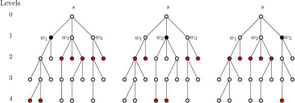
Figure 2: Relation between nodes at distance 4 for $s$ and the neighbors of $s$. The red nodes represent the nodes at distance 3 for $w_{1}$ (left), for $w_{2}$ (center) and for $w_{3}$ (right).

Figure 2 shows an example where $s$ has three neighbors $w_{1}$, $w_{2}$ and $w_{3}$. Suppose we want to compute $\Gamma_{4}(s)$ using information from $w_{1}$, $w_{2}$ and $w_{3}$. Clearly, $\Gamma_{4}(s)\subset\Gamma_{3}(w_{1})\cup\Gamma_{3}(w_{2})\cup\Gamma_{3}(w_{3})$; however, there are also other nodes in the union that are not in $\Gamma_{4}(s)$. Furthermore, the nodes in $\Gamma_{3}(w_{1})$ (red nodes in the leftmost tree) are of two types: nodes in $\Gamma_{4}(s)$ (the ones in the subtree of $w_{1}$) and nodes in $\Gamma_{2}(s)$ (the ones in the subtrees of $w_{2}$ and $w_{3}$). An analogous behavior can be observed for $w_{2}$ and $w_{3}$ (central and rightmost trees). If we simply sum all the nodes in $\gamma_{3}(w_{1})$, $\gamma_{3}(w_{2})$ and $\gamma_{3}(w_{3})$, we would be counting each node at level 2 twice, i. e. once for each node in $\Gamma_{1}(s)$ minus one. Hence, for each $k>2$, we can write

$$\gamma_{k}(s)=\sum_{w\in\Gamma_{1}(s)}\gamma_{k-1}(w)-\gamma_{k-2}(s)\cdot(\operatorname{deg}(s)-1).$$ (2)

Input : A tree $T=(V,E)$

Output : Closeness centralities $c(v)$ of each node $v\in V$

1 foreach $s\in V$ do

2       $\textnormal{{$\gamma_{k-1}(s)$}}\leftarrow\operatorname{deg}(s)$;

3       $\textnormal{{$S$}}(s)\leftarrow\operatorname{deg}(s)$;

4      

5$\textnormal{{k}}\leftarrow 2$;

6 $\textnormal{{nFinished}}\leftarrow 0$;

7 while $\textnormal{{nFinished}}<n$ do

8       foreach $s\in V$ do

9             if $\textnormal{{k}}=2$  then

10                   $\textnormal{{$\gamma_{k}(s)$}}\leftarrow\sum_{w\in N(s)}\textnormal{{$\gamma_{k-1}(w)$}}-\operatorname{deg}(s)$;

11                  

12            else

13                   $\textnormal{{$\gamma_{k}(s)$}}\leftarrow\sum_{w\in N(s)}\textnormal{{$\gamma_{k-1}(w)$}}-\textnormal{{$\gamma_{k-2}(s)$}}(\operatorname{deg}(s)-1)$;

14                  

15            

16      foreach $s\in V$ do

17             $\textnormal{{$\gamma_{k-2}(s)$}}\leftarrow\textnormal{{$\gamma_{k-1}(s)$}}$;

18             $\textnormal{{$\gamma_{k-1}(s)$}}\leftarrow\textnormal{{$\gamma_{k}(s)$}}$;

19             if $\textnormal{{$\gamma_{k-1}(s)$}}>0$ then

20                   $\textnormal{{$S$}}(s)\leftarrow\textnormal{{$S$}}(s)+\textnormal{{k}}\cdot\textnormal{{$\gamma_{k-1}(s)$}}$;

21                  

22            else

23                   $\textnormal{{nFinished}}\leftarrow\textnormal{{nFinished}}+1$;

24                  

25            

26      $\textnormal{{k}}\leftarrow\textnormal{{k}}+1$;

27      

28foreach $s\in V$ do

29       $c(v)\leftarrow(n-1)/\textnormal{{$S$}}(v)$;

30      

return $c$

ALGORITHM 2 Closeness centrality in trees

From this observation, we define a new method to compute the total distance of all nodes, described in Algorithm 2. Instead of computing the BFS tree of each node one by one, at each step we compute the number $\gamma_{k}(v)$ of nodes at level $k$ for all nodes $v$. First (Lines 2 - 2), we compute $\gamma_{1}(v)$ for each node (and add that to $S(v)$). Then (Lines 2 - 2), we consider all the other levels $k$ one by one. For each $k$, we use $\gamma_{k-1}(w)$ of the neighbors $w$ of $v$ and $\gamma_{k-2}(v)$ to compute $\gamma_{k}(v)$ (Line 2 and 2). If, for some $k$, $\gamma_{k}(v)=0$, all the nodes have been added to $S(v)$. Therefore, we can stop the algorithm when $\gamma_{k}(v)=0\ \ \forall v\in V$.

Proposition 5.3.

Algorithm 2 requires $O(D\cdot n)$ operations to compute the closeness centrality of all nodes in a tree $T$.

Proof 5.4.

The for loop in Lines 2 - 2 of Algorithm 2 clearly takes $O(n)$ time. For each level of the while loop of Lines 2 - 2, each node scans its neighbors in Line 2 or Line 2. In total, this leads to $O(n)$ operations per level since $m=O(n)$. Since the maximum number of levels that a node can have is equal to the diameter of the tree, the algorithm requires $O(D\cdot n)$ operations. ∎

Note that closeness centrality on trees could even be computed in time $O(n)$ in a different manner [Brandes and Fleischer (2005)]. We choose to include Algorithm 2 here nonetheless since it paves the way for an algorithm computing a lower bound in general undirected graphs, described next.

Lower bound for undirected graphs

For general undirected graphs, Eq. (2) is not true anymore – but a related upper bound $\tilde{\gamma}_{k}(\cdot)$ on $\gamma_{k}(\cdot)$ is still useful. Let $\tilde{\gamma}_{k}(s)$ be defined recursively as in Eq. (2): in a tree, $\tilde{\gamma}_{k}(s)=\gamma_{k}(s)$, while in this case we prove that $\tilde{\gamma}_{k}(s)$ is an upper bound on $\Gamma_{k}(s)$. Indeed, there could be nodes $x$ for which there are multiple paths between $s$ and $x$ and that are therefore contained in the subtrees of more than one neighbor of $s$. This means that we would count $x$ multiple times when considering $\tilde{\gamma}_{k}(s)$, overestimating the number of nodes at distance $k$. However, we know for sure that at level $k$ there cannot be more nodes than in Eq. (2). If, for each node $v$, we assume that the number $\tilde{\gamma}_{k}(v)$ of nodes at distance $k$ is that of Eq. (2), we can apply Prop. 5.1 and get a lower bound $S^{\text{NB}}(v,r(v))$ on the total sum for undirected graphs. The procedure is described in Algorithm 3. The computation of $S^{\text{NB}}(v,r(v))$ works basically like Algorithm 2, with the difference that here we keep track of the number of the nodes found in all the levels up to $k$ (nVisited) and stop the computation when nVisited becomes equal to $r(v)$ (if it becomes larger, in the last level we consider only $r(v)-\textsf{nVisited}$ nodes, as in Prop. 5.1 (Lines 3 - 3).

Proposition 5.5.

For an undirected graph $G$, computing the lower bound $S^{\text{NB}}(v,r(v))$ described in Algorithm 3 takes $O(D\cdot m)$ time.

Proof 5.6.

Like in Algorithm 2, the number of operations performed by Algorithm 3 at each level of the while loop is $\mathcal{O}(m)$. At each level $i$, all the nodes at distance $i$ are accounted for (possibly multiple times) in Lines 3 and 3. Therefore, at each level, the variable $\mathsf{nVisited}$ is always greater than or equal to the the number of nodes $v$ at distance $d(v)\leq i$. Since $d(v)\leq D$ for all nodes $v$, the maximum number of levels scanned in the while loop cannot be larger than $D$, therefore the total complexity is $O(D\cdot m)$. ∎

Input : A graph $G=(V,E)$

Output : Lower bounds $L^{\text{NB}}(v,r(v))$ of each node $v\in V$

1 foreach $s\in V$ do

2       $\textnormal{{$\gamma_{k-1}(s)$}}\leftarrow\operatorname{deg}(s)$;

3       $\textnormal{{$\tilde{S}^{\mathrm{(un)}}$}}(s)\leftarrow\operatorname{deg}(s)$;

4       $\textnormal{{nVisited}}[s]\leftarrow\operatorname{deg}(s)+1$;

5       $\textnormal{{finished}}[s]\leftarrow false$;

6      

7$\textnormal{{$k$}}\leftarrow 2$;

8 $\textnormal{{nFinished}}\leftarrow 0$;

9

10while $\textnormal{{nFinished}}<n$ do

11       foreach $s\in V$ do

12             if $\textnormal{{$k$}}=2$  then

13                   $\textnormal{{$\gamma_{k}(s)$}}\leftarrow\sum_{w\in N(s)}\textnormal{{$\gamma_{k-1}(w)$}}-\operatorname{deg}(s)$;

14                  

15            else

16                   $\textnormal{{$\gamma_{k}(s)$}}\leftarrow\sum_{w\in N(s)}\textnormal{{$\gamma_{k-1}(w)$}}-\textnormal{{$\gamma_{k-2}(s)$}}(\operatorname{deg}(s)-1)$;

17                  

18            

19      foreach $s\in V$ do

20             if $\textnormal{{finished}}[v]$ then

21                   continue;

22                  

23            $\textnormal{{$\gamma_{k-2}(s)$}}\leftarrow\textnormal{{$\gamma_{k-1}(s)$}}$;

24             $\textnormal{{$\gamma_{k-1}(s)$}}\leftarrow\textnormal{{$\gamma_{k}(s)$}}$;

25             $\textnormal{{nVisited}}[s]\leftarrow\textnormal{{nVisited}}[s]+\textnormal{{$\gamma_{k-1}(s)$}}$;

26             if $\textnormal{{nVisited}}[s]<r(v)$ then

27                   $\textnormal{{$\tilde{S}^{\mathrm{(un)}}$}}(s)\leftarrow\textnormal{{$\tilde{S}^{\mathrm{(un)}}$}}(s)+\textnormal{{$k$}}\cdot\textnormal{{$\gamma_{k-1}(s)$}}$;

28                  

29            else

30                   $\textnormal{{$\tilde{S}^{\mathrm{(un)}}$}}(s)\leftarrow\textnormal{{$\tilde{S}^{\mathrm{(un)}}$}}(s)+\textnormal{{$k$}}(r(v)-(\textnormal{{nVisited}}[s]-\textnormal{{$\gamma_{k-1}(s)$}}))$;

31                   $\textnormal{{nFinished}}\leftarrow\textnormal{{nFinished}}+1$;

32                   $\textnormal{{finished}}[s]\leftarrow true$;

33                  

34            

35      $\textnormal{{$k$}}\leftarrow\textnormal{{$k$}}+1$;

36      

37foreach $v\in v$ do

38       $L^{\text{NB}}(v,r(v))\leftarrow\frac{(n-1)\tilde{S}^{\mathrm{(un)}}}{(r(v)-1)^{2}}$;

39      

return $L^{\text{NB}}(\cdot,r(\cdot))$

ALGORITHM 3 Neighborhood-based lower bound for undirected graphs

Lower bound on directed graphs

In directed graphs, we can simply consider the out-neighbors, without subtracting the number of nodes discovered in the subtrees of the other neighbors in Eq. (2). The lower bound (which we still refer to as $S^{\text{NB}}(v,r(v))$) is obtained by replacing Eq. (2) with the following in Lines 3 and 3 of Algorithm 3:

$$\tilde{\gamma}_{k}(s)=\sum_{w\in\Gamma(s)}\tilde{\gamma}_{k-1}(w)$$ (3)

6 The updateBoundsBFSCut Function

The updateBoundsBFSCut function is based on a simple idea: if the $k$-th biggest farness found until now is $x$, and if we are performing a BFS from vertex $v$ to compute its farness $f(v)$, we can stop as soon as we can guarantee that $f(v)\geq x$.

Informally, assume that we have already visited all nodes up to distance $d$: we can lower bound $S(v)=\sum_{w\in V}d(v,w)$ by setting distance $d+1$ to a number of vertices equal to the number of edges “leaving” level $d$, and distance $d+2$ to all the remaining reachable vertices. Then, this bound yields a lower bound on the farness of $v$. As soon as this lower bound is bigger than $x$, the updateBoundsBFSCut function may stop; if this condition never occurs, at the end of the BFS we have exactly computed the farness of $x$.

More formally, the following lemma defines a lower bound $S^{\text{CUT}}_{d}(v,r(v))$ on $S(v)$, which is computable after we have performed a BFS from $v$ up to level $d$, assuming we know the number $r(v)$ of vertices reachable from $v$ (this assumption is lifted in Sect. 8).

Lemma 6.1.

Given a graph $G=(V,E)$, a vertex $v\in V$, and an integer $d\geq 0$, let $N_{d}(v)$ be the set of vertices at distance at most $d$ from $v$, $n_{d}(v)=|N_{d}(v)|$, and let $\tilde{\gamma}_{d+1}(v)$ be an upper bound on the number of vertices at distance $d+1$ from $v$ (see Table 2). Then,

$$S(v)\geq S^{\text{CUT}}_{d}(v,r(v)):=\sum_{w\in N_{d}(v)}d(v,w)-\tilde{\gamma}_{d+1}(v)+(d+2)(r(v)-n_{d}(v)).$$

Proof 6.2.

The sum of all the distances from $v$ is lower bounded by setting the correct distance to all vertices at distance at most $d$ from $v$, by setting distance $d+1$ to all vertices at distance $d+1$ (there are $\gamma_{d+1}(v)$ such vertices), and by setting distance $d+2$ to all other vertices (there are $r(v)-n_{d+1}(v)$ such vertices, where $r(v)$ is the number of vertices reachable from $v$ and $n_{d+1}(v)$ is the number of vertices at distance at most $d+1$). More formally, $f(v)\geq\sum_{w\in N_{d}(v)}d(v,w)+(d+1)\gamma_{d+1}(v)+(d+2)(r(v)-n_{d+1}(v)).$

Since $n_{d+1}(v)=\gamma_{d+1}(v)+n_{d}(v)$, we obtain that $f(v)\geq\sum_{w\in N_{d}(v)}d(v,w)-\gamma_{d+1}(v)+(d+2)(r(v)-n_{d}(v))$. We conclude because, by assumption, $\tilde{\gamma}_{d+1}(v)$ is an upper bound on $\gamma_{d+1}(v)$. ∎

Corollary 6.3.

For each vertex $v$ and for each $d\geq 0$,

$$f(v)\geq L^{\text{CUT}}_{d}(v,r(v)):=\frac{(n-1)S^{\text{CUT}}_{d}(v,r(v))}{(r(v)-1)^{2}}.$$

It remains to define the upper bound $\tilde{\gamma}_{d+1}(v)$: in the directed case, this bound is simply the sum of the out-degrees of vertices at distance $d$ from $v$. In the undirected case, since at least an edge from each vertex $v\in\Gamma_{d}(v)$ is directed towards $\Gamma_{d-1}(v)$, we may define $\tilde{\gamma}_{d+1}(v)=\sum_{w\in\Gamma_{d}(v)}\deg(w)-1$ (the only exception is $d=0$: in this case, $\tilde{\gamma}_{1}(v)=\gamma_{1}(v)=\deg(v)$).

Remark 6.4.

When we are processing vertices at level $d$, if we process an edge $(x,y)$ where $y$ is already in the BFS tree, we can decrease $\tilde{\gamma}_{d+1}(v)$ by one, obtaining a better bound.

Assuming we know $r(v)$, all quantities necessary to compute $L^{\text{CUT}}_{d}(v,r(v))$ are available as soon as all vertices in $N_{d}(v)$ are visited by a BFS. This function performs a BFS starting from $v$, continuously updating the upper bound $L^{\text{CUT}}_{d}(v,r(v))\leq f(v)$ (the update is done whenever all nodes in $\Gamma_{d}(v)$ have been reached, or Remark 6.4 can be used). As soon as $L^{\text{CUT}}_{d}(v,r(v))\geq x$, we know that $f(v)\geq L^{\text{CUT}}_{d}(v,r(v))\geq x$, and we return $+\infty$.

Algorithm 4 is the pseudocode of the function updateBoundsBFSCut when implemented for directed graphs, assuming we know the number $r(v)$ of vertices reachable from each $v$ (for example, if the graph is strongly connected). This code can be easily adapted to all the other cases.

1 $x\leftarrow\textnormal{{Farn}}(\textnormal{{Top}}[k])$; // Farn and Top are global variables, as in Algorithm 1.

2 Create queue $Q$;

3 $Q$.enqueue($v$);

4 Mark $v$ as visited;

5 $d\leftarrow 0$; $S\leftarrow 0$; $\tilde{\gamma}\leftarrow\operatorname{outdeg}(v)$; $nd\leftarrow 1$;

6 while $Q$ is not empty do

7       $u\leftarrow Q$.dequeue();

8       if $d(v,u)>d$ then

9             $d\leftarrow d+1$;

10             $L^{\text{CUT}}_{d}(v,r(v))\leftarrow\frac{(n-1)\left(S-\tilde{\gamma}+(d+2)(r(v)-nd)\right)}{(r(v)-1)^{2}}$;

11             if $L^{\text{CUT}}_{d}(v,r(v))\geq x$ then return $+\infty$;

12             $\tilde{\gamma}\leftarrow 0$

13      for $w$ in adjacency list of $u$ do

14             if $w$ is not visited then

15                   $S\leftarrow S+d(v,w)$;

16                   $\tilde{\gamma}\leftarrow\tilde{\gamma}+\mathrm{outdeg}(w)$;

17                   $nd\leftarrow nd+1$;

18                   $Q$.enqueue($w$);

19                   Mark $w$ as visited

20            else

21                   // we use Remark 6.4

22                   $L^{\text{CUT}}_{d}(v,r(v))\leftarrow L^{\text{CUT}}_{d}(v,r(v))+\frac{(n-1)}{(r(v)-1)^{2}}$;

23                   if $L^{\text{CUT}}_{d}(v,r(v))\geq x$ then return $x$;

24                  

25            

26      

return $\frac{S(n-1)}{(r(v)-1)^{2}}$;

ALGORITHM 4 The updateBoundsBFSCut$(v)$ function in the case of directed graphs, if $r(v)$ is known for each $v$.

7 The updateBoundsLB Function

Differently from updateBoundsBFSCut function, updateBoundsLB computes a complete BFS traversal, but uses information acquired during the traversal to update the bounds on the other nodes. Let us first consider an undirected graph $G$ and let $s$ be the source node from which we are computing the BFS. We can see the distances $d(s,v)$ between $s$ and all the nodes $v$ reachable from $s$ as levels: node $v$ is at level $i$ if and only if the distance between $s$ and $v$ is $i$, and we write $v\in\Gamma_{i}(s)$ (or simply $v\in{\Gamma}_{i}$ if $s$ is clear from the context). Let $i$ and $j$ be two levels, $i\leq j$. Then, the distance between any two nodes $v$ at level $i$ and $w$ at level $j$ must be at least $j-i$. Indeed, if $d(v,w)$ was smaller than $j-i$, $w$ would be at level $i+d(v,w)<j$, which contradicts our assumption. It follows directly that $\sum_{w\in V}|d(s,w)-d(s,v)|$ is a lower bound on $S(v)$, for all $v\in R(s)$:

Lemma 7.1.

$\sum_{w\in R(s)}|d(s,w)-d(s,v)|\leq S(v)\quad\forall v\in R(s)$.

To improve the approximation, we notice that the number of nodes at distance 1 from $v$ is exactly the degree of $v$. Therefore, all the other nodes $w$ such that $|d(s,v)-d(s,w)|\leq 1$ must be at least at distance 2 (with the only exception of $v$ itself, whose distance is of course 0). This way we can define the following lower bound on $S(v)$:

$$2(\#\{w\in R(s):|d(s,w)-d(s,v)|\leq 1\}-\operatorname{deg}(v)-1)+$$

$$+\operatorname{deg}(v)+\sum\limits_{\begin{subarray}{c}w\in R(s)\\ |d(s,w)-d(s,v)|>1\end{subarray}}|d(s,w)-d(s,v)|,$$

that is:

$$2\cdot\sum_{|j-d(s,v)|\leq 1}{\gamma}_{j}+\sum_{|j-d(s,v)|>1}{\gamma}_{j}\cdot|j-d(s,v)|-\operatorname{deg}(v)-2,$$ (4)

where ${\gamma}_{j}=|{\Gamma}_{j}{}|$.

Multiplying the bound of Eq. (LABEL:eq:lbound1) by $\frac{(n-1)}{(r(v)-1)^{2}}$, we obtain a lower bound on the farness $f(v)$ of node $v$, named $L^{\text{LB}}_{s}(v,r(v))$. A straightforward way to compute $L^{\text{LB}}_{s}(v,r(v))$ would be to first run the BFS from $s$ and then, for each node $v$, to consider the level difference between $v$ and all the other nodes. This would require $\mathcal{O}(n^{2})$ operations, which is clearly too expensive. However, we can notice two things: First, the bounds of two nodes at the same level differ only by their degree. Therefore, for each level $i$, we can compute $2\cdot\sum_{|j-i|\leq 1}{\gamma}_{j}+\sum_{|j-i|>1}{\gamma}_{j}\cdot|j-i|-2$ only once and then subtract $\operatorname{deg}(v)$ for each node at level $i$. We call the quantity $2\cdot\sum_{|j-i|\leq 1}{\gamma}_{j}+\sum_{|j-i|>1}{\gamma}_{j}\cdot|j-i|-2$ the level-bound $\mathsf{L}(i)$ of level $i$. Second, we can prove that $\mathsf{L}(i)$ can actually be written as a function of $\mathsf{L}(i-1)$.

Lemma 7.2.

Let $\mathsf{L}(i):=2\cdot\sum_{|j-i|\leq 1}{\gamma}_{j}+\sum_{|j-i|>1}{\gamma}_{j}\cdot|j-i|-2$. Also, let ${\gamma}_{j}=0$ for $j\leq 0$ and $j>\mathsf{maxD}$, where $\mathsf{maxD}=\max_{v\in R(s)}d(s,v)$. Then $\mathsf{L}(i)-\mathsf{L}(i-1)=\sum_{j<i-2}{\gamma}_{j}-\sum_{j>i+1}{\gamma}_{j}$, $\forall i\in\{1,...,\mathsf{maxD}\}$.

Proof 7.3.

Since ${\gamma}_{j}=0$ for $j\leq 0$ and $j>\mathsf{maxD}$, we can write $\mathsf{L}(i)$ as $2\cdot({\gamma}_{i-1}+{\gamma}_{i}+{\gamma}_{i+1})+\sum_{|j-i|>1}{\gamma}_{j}\cdot|j-i|-2$, $\forall i\in\{1,...,\mathsf{maxD}\}$. The difference between $\mathsf{L}(i)$ and $\mathsf{L}(i-1)$ is: $2\cdot({\gamma}_{i-1}+{\gamma}_{i}+{\gamma}_{i+1})+\sum_{|j-i|>1}|j-i|\cdot{\gamma}_{j}-2\cdot({\gamma}_{i-2}+{\gamma}_{i-1}+{\gamma}_{i})+\sum_{|j-i+1|>1}|j-i+1|\cdot{\gamma}_{j}=2\cdot({\gamma}_{i+1}-{\gamma}_{i-2})+2\cdot{\gamma}_{i-2}-2\cdot{\gamma}_{i+1}+\sum_{j<i-2\cup j>i+1}(|j-i|-|j-i+1|)\cdot{\gamma}_{j}=\sum_{j<i-2}{\gamma}_{j}-\sum_{j>i+1}{\gamma}_{j}$. ∎

Input : A graph $G=(V,E)$, a source node $s$

Output : Lower bounds $L^{\text{LB}}_{s}(v,r(v))$ of each node $v\in R(s)$

1 $d\leftarrow\textnormal{{BFSfrom(}}\textnormal{\emph{s}}\textnormal{{)}}$;

2 $\textnormal{{maxD}}\leftarrow\max_{v\in V}d(s,v)$;

3 $\textnormal{{sum$\Gamma$}}_{\leq 0}\leftarrow 0$; $\textnormal{{sum$\Gamma$}}_{\leq-1}\leftarrow 0$; $\textnormal{{sum$\Gamma$}}_{>{\textnormal{{maxD}}+1}}\leftarrow 0$;

4 for $i=1,2,...,\textnormal{{maxD}}$ do

5       ${\Gamma}_{i}\leftarrow\{w\in V:d(s,w)=i\}$;

6       ${\gamma}_{i}\leftarrow\#{\Gamma}_{i}$;

7       $\textnormal{{sum$\Gamma$}}_{\leq i}\leftarrow\textnormal{{sum$\Gamma$}}_{\leq i-1}+{\gamma}_{i}$;

8       $\textnormal{{sum$\Gamma$}}_{>i}\leftarrow|V|-\textnormal{{sum$\Gamma$}}_{\leq i}$;

9      

10 $\mathsf{L}(1)\leftarrow{\gamma}_{1}+{\gamma}_{2}+\textnormal{{sum$\Gamma$}}_{>2}-2$;

11 for $i=2,...,\textnormal{{maxD}}$ do

12       $\mathsf{L}(i)\leftarrow\mathsf{L}(i-1)+\textnormal{{sum$\Gamma$}}_{\leq i-3}-\textnormal{{sum$\Gamma$}}_{>i+1}$;

13      

14for $i=1,...,\textnormal{{maxD}}$ do

15       foreach $v\in{\Gamma}_{i}$ do

16             $L^{\text{LB}}_{s}(v,r(v))\leftarrow(\mathsf{L}(i)-\operatorname{deg}(v))\cdot\frac{(n-1)}{(r(v)-1)^{2}}$;

17            

18      

return $L^{\text{LB}}_{s}(v,r(v))\quad\forall v\in V$

ALGORITHM 5 The updateBoundsLB function for undirected graphs

Algorithm 5 describes the computation of $L^{\text{LB}}_{s}(v,r(v))$. First, we compute all the distances between $s$ and the nodes in $R(s)$ with a BFS, storing the number of nodes in each level and the number of nodes in levels $j\leq i$ and $j>i$ respectively (Lines 5 - 5). Then we compute the level bound $\mathsf{L}(1)$ of level $1$ according to its definition (Line 5) and those of the other level according to Lemma 7.2 (Line 5). The lower bound $L^{\text{LB}}_{s}(v,r(v))$ is then computed for each node $v$ by subtracting its degree to $\mathsf{L}(d(s,v))$ and normalizing (Line 5). The complexity of Lines 5 - 5 is that of running a BFS, i. e. $\mathcal{O}(n+m)$. Line 5 is repeated once for each level (which cannot be more than $n$) and Line 5 is repeated once for each node in $R(s)$. Therefore, the following proposition holds.

Proposition 7.4.

Computing the lower bound $L^{\text{LB}}_{s}(v,r(v))$ takes $\mathcal{O}(n+m)$ time.

For directed strongly-connected graphs, the result does not hold for nodes $w$ whose level is smaller than $l(v)$, since there might be a directed edge or a shortcut from $v$ to $w$. Yet, for nodes $w$ such that $d(s,w)>d(s,v)$, it is still true that $d(v,w)\geq d(s,w)-d(s,v)$. For the remaining nodes (apart from the outgoing neighbors of $v$), we can only say that the distance must be at least 2. The upper bound $L^{\text{LB}}_{s}(v,r(v))$ for directed graphs can therefore be defined as:

$$2\cdot\#\{w\in R(s):d(s,w)-d(s,v)\leq 1\}$$ (5)

$$+\sum\limits_{\begin{subarray}{c}w\in R(s)\\ d(s,w)-d(s,v)>1\end{subarray}}(d(s,w)-d(s,v))-\operatorname{deg}(v)-2.$$

The computation of $L^{\text{LB}}_{s}(v,r(v))$ for directed strongly-connected graphs is analogous to the one described in Algorithm 5.

8 The Directed Disconnected Case

In the directed disconnected case, even if the time complexity of computing strongly connected components is linear in the input size, the time complexity of computing the number of reachable vertices is much bigger (assuming SETH, it cannot be $\mathcal{O}(m^{2-\epsilon})$ [Borassi (2016)]). For this reason, when computing our upper bounds, we cannot rely on the exact value of $r(v)$: for now, let us assume that we know a lower bound $\alpha(v)\leq r(v)$ and an upper bound $\omega(v)\geq r(v)$. The definition of these bounds is postponed to Sect. 8.4.

Furthermore, let us assume that we have a lower bound $L(v,r(v))$ on the farness of $v$, depending on the number $r(v)$ of vertices reachable from $v$: in order to obtain a bound not depending on $r(v)$, the simplest approach is $f(v)\geq L(v,r(v))\geq\min_{\alpha(v)\leq r\leq\omega(v)}L(v,r)$. However, during the algorithm, computing the minimum among all these values might be quite expensive, if $\omega(v)-\alpha(v)$ is big. In order to solve this issue, we find a small set $X\subseteq[\alpha(v),\omega(v)]$ such that $\min_{\alpha(v)\leq r\leq\omega(v)}L(v,r)=\min_{r\in X}L(v,r)$.

More specifically, we find a condition that is verified by “many” values of $r$, and that implies $L(v,r)\geq\min\left(L(v,r-1),L(v,r+1)\right)$: this way, we may define $X$ as the set of values of $r$ that either do not verify this condition, or that are extremal points of the interval $[\alpha(v),\omega(v)]$ (indeed, all other values cannot be minima of $L(v,r)$). Since all our bounds are of the form $L(v,r)=\frac{(n-1)S(v,r)}{(r-1)^{2}}$, where $S(v,r)$ is a lower bound on $\sum_{w\in R(v)}d(v,w)$, we state our condition in terms of the function $S(v,r)$. For instance, in the case of the updateBoundsBFSCut function, $S^{\text{CUT}}_{d}(v,r)=\sum_{w\in N_{d}(v)}d(v,w)-\tilde{\gamma}_{d+1}(v)+(d+2)(r-n_{d}(v))$, as in Lemma 6.1.

Lemma 8.1.

Let $v$ be a vertex, and let $S(v,r)$ be a positive function such that $S(v,r(v)))\leq\sum_{w\in R(v)}d(v,w)$ (where $r(v)$ is the number of vertices reachable from $v$). Assume that $S(v,r+1)-S(v,r)\leq S(v,r)-S(v,r-1)$. Then, if $L(v,r):=\frac{(n-1)S(v,r)}{(r-1)^{2}}$ is the corresponding bound on the farness of $v$, $\min\left(L(v,r+1),L(v,r-1)\right)\leq L(v,r)$.

Proof 8.2.

Let us define $d=S(v,r+1)-S(v,r)$. Then, $L(v,r+1)\leq L(v,r)$ if and only if $\frac{(n-1)S(v,r+1)}{r^{2}}\leq\frac{(n-1)S(v,r)}{(r-1)^{2}}$ if and only if $\frac{S(v,r)+d}{r^{2}}\leq\frac{S(v,r)}{(r-1)^{2}}$ if and only if $(r-1)^{2}(S(v,r)+d)\leq r^{2}S(v,r)$ if and only if $S(v,r)(r^{2}-(r-1)^{2})\geq(r-1)^{2}d$ if and only if $S(v,r)(2r-1)\geq(r-1)^{2}d$.

Similarly, if $d^{\prime}=S(v,r)-S(v,r-1)$, $L(v,r-1)\leq L(v,r)$ if and only if $\frac{(n-1)S(v,r-1)}{(r-2)^{2}}\leq\frac{(n-1)S(v,r)}{(r-1)^{2}}$ if and only if $\frac{S(v,r)-d^{\prime}}{(r-2)^{2}}\leq\frac{S(v,r)}{(r-1)^{2}}$ if and only if $(r-1)^{2}(S(v,r)-d^{\prime})\leq(r-2)^{2}S(v,r)$ if and only if $S(v,r)((r-1)^{2}-(r-2)^{2})\leq(r-1)^{2}d^{\prime}$ if and only if $S(v,r)(2r-3)\leq(r-1)^{2}d^{\prime}$ if and only if $S(v,r)(2r-1)\leq(r-1)^{2}d^{\prime}+2S(v,r)$.

We conclude that, assuming $d\leq d^{\prime}$, $(r-1)^{2}d\leq(r-1)^{2}d^{\prime}\leq(r-1)^{2}d+2S(v,r)$, and one of the two previous conditions is always satisfied.∎

8.1 The Neighborhood-Based Lower Bound

In the neighborhood-based lower bound, we computed upper bounds $\tilde{\gamma}_{k}(v)$ on $\Gamma_{k}(v)$, and we defined the lower bound $S^{\text{NB}}(v,r(v))\leq\sum_{w\in R(v)}d(v,w)$, by

$$S^{\text{NB}}(v,r(v)):=\sum_{k=1}^{\operatorname{diam}(G)}k\cdot\min\left\{\tilde{\gamma}_{k}(v),\ r(v)-\sum_{i=0}^{k-1}\tilde{\gamma}_{i}(v),\ 0\right\}.$$

The corresponding bound on $f(v)$ is $L^{\text{NB}}(v,r(v)):=\frac{(n-1)S^{\text{NB}}(v,r(v))}{(r(v)-1)^{2}}$: let us apply Lemma 8.1 with $S(v,r)=S^{\text{NB}}(v,r)$ and $L(v,r)=L^{\text{NB}}(v,r)$. We obtain that the local minima of $L^{\text{NB}}(v,r(v))$ are obtained on values $r$ such that $S^{\text{NB}}(v,r+1)-S^{\text{NB}}(v,r)>S^{\text{NB}}(v,r)-S^{\text{NB}}(v,r-1)$, that is, when $r=\sum_{i=0}^{l}\tilde{\gamma}_{i}(v)$ for some $l$. Hence, our final bound $L^{\text{NB}}(v)$ becomes:

$$\min\left(L^{\text{NB}}(v,\alpha(v)),L^{\text{NB}}(v,\omega(v)),\min\left\{L^{\text{NB}}(v,r):\alpha(v)<r<\omega(v),r=\sum_{i=0}^{l}\tilde{\gamma}_{i}(v)\right\}\right).$$ (6)

This bound can be computed with no overhead, by modifying Lines 3 - 3 in Algorithm 3. Indeed, when $r(v)$ is known, we have two cases: either $\texttt{nVisited[s]}<r(v)$, and we continue, or $\texttt{nVisited[s]}\geq r(v)$, and $S^{\text{NB}}(v,r(v))$ is computed. In the disconnected case, we need to distinguish three cases:

• if $\texttt{nVisited[v]}<\alpha(v)$, we simply continue the computation;

• if $\alpha(v)\leq\texttt{nVisited[v]}<\omega(v)$, we compute $L^{\text{NB}}(v,\texttt{nVisited[v]})$, and we update the minimum in Eq. 6 (if this is the first occurrence of this situation, we also have to compute $L^{\text{NB}}(v,\alpha(v))$);

• if $\texttt{nVisited[v]}\geq\omega(v)$, we compute $L^{\text{NB}}(v,\omega(v))$, and we update the minimum in Eq. 6.

Since this procedure needs time $\mathcal{O}(1)$, it has no impact on the running time of the computation of the neighborhood-based lower bound.

8.2 The updateBoundsBFSCut Function

Let us apply Lemma 8.1 to the bound used in the updateBoundsBFSCut function. In this case, by Lemma 6.1, $S^{\text{CUT}}_{d}(v,r)=\sum_{w\in N_{d}(v)}d(v,w)-\tilde{\gamma}_{d+1}(v)+(d+2)(r-n_{d}(v))$, and $S^{\text{CUT}}_{d}(v,r+1)-S^{\text{CUT}}_{d}(v,r)=d+2$, which does not depend on $r$. Hence, the condition in Lemma 8.1 is always verified, and the only values we have to analyze are $\alpha(v)$ and $\omega(v)$. Hence, the lower bound becomes $f(v)\geq L^{\text{CUT}}_{d}(v,r(v))\geq\min_{\alpha(v)\leq r\leq\omega(v)}L^{\text{CUT}}_{d}(v,r)=\min(L^{\text{CUT}}_{d}(v,\alpha(v)),L^{\text{CUT}}_{d}(v,\omega(v)))$ (which does not depend on $r(v)$).

This means that, in order to adapt the updateBoundsBFSCut function (Algorithm 4), it is enough to replace Lines 4, 4 in order to compute both $L^{\text{CUT}}_{d}(v,\alpha(v))$ and $L^{\text{CUT}}_{d}(v,\omega(v)))$, and to replace Lines 4, 4 in order to stop if $\min(L^{\text{CUT}}_{d}(v,\alpha(v)),L^{\text{CUT}}_{d}(v,\omega(v)))\geq x$.

8.3 The updateBoundsLB Function

In this case, we do not apply Lemma 8.1 to obtain simpler bounds. Indeed, the updateBoundsLB function improves the bounds of vertices that are quite close to the source of the BFS, and hence are likely to be in the same component as this vertex. Consequently, if we perform a BFS from a vertex $s$, we can simply compute $L^{\text{LB}}_{s}(v,r(v))$ for all vertices in the same strongly connected component as $s$, and for these vertices we know the value $r(v)=r(s)$. The computation of better bounds for other vertices is left as an open problem.

8.4 Computing $\alpha(v)$ and $\omega(v)$

It now remains to compute $\alpha(v)$ and $\omega(v)$. This can be done during the preprocessing phase of our algorithm, in linear time. To this purpose, let us precisely define the node-weighted directed acyclic graph $\mathcal{G=(V,E)}$ of strongly connected components (in short, SCCs) corresponding to a directed graph $G=(V,E)$. In this graph, $\mathcal{V}$ is the set of SCCs of $G$, and, for any two SCCs $C,D\in\mathcal{V}$, $(C,D)\in\mathcal{E}$ if and only if there is an arc in $E$ from a node in $C$ to the a node in $D$. For each SCC $C\in\mathcal{V}$, the weight $w(C)$ of $C$ is equal to $|C|$, that is, the number of nodes in the SCC $C$. Note that the graph $\mathcal{G}$ is computable in linear time.

For each node $v\in C$, $r(v)=\sum_{D\in R(C)}w(D)$, where $R(C)$ denotes the set of SCCs that are reachable from $C$ in $\mathcal{G}$. This means that we simply need to compute a lower (respectively, upper) bound $\alpha_{SCC}(C)$ (respectively, $\omega_{SCC}(C)$) on $\sum_{D\in\mathcal{R}(C)}w(D)$, for every SCC $C$. To this aim, we first compute a topological sort $\{C_{1},\dots,C_{l}\}$ of $\mathcal{V}$ (that is, if $(C_{i},C_{j})\in\mathcal{E}$, then $i<j$). Successively, we use a dynamic programming approach, and, by starting from $C_{l}$, we process the SCCs in reverse topological order, and we set:

$$\alpha_{SCC}(C)=w(C)+\max_{(C,D)\in\mathcal{E}}\alpha_{SCC}(D)\quad\,\,\omega_{SCC}(C)=w(C)+\sum_{(C,D)\in\mathcal{E}}\omega_{SCC}(D).$$

Note that processing the SCCs in reverse topological ordering ensures that the values $\alpha(D)$ and $\omega(D)$ on the right hand side of these equalities are available when we process the SCC $C$. Clearly, the complexity of computing $\alpha(C)$ and $\omega(C)$, for each SCC $C$, is linear in the size of $\mathcal{G}$, which in turn is smaller than $G$.

Observe that the bounds obtained through this simple approach can be improved by using some “tricks”. First of all, when the biggest SCC $\tilde{C}$ is processed, we do not use the dynamic programming approach and we exactly compute $\sum_{D\in\mathcal{R}(\tilde{C})}w(D)$ by performing a BFS starting from any node in $\tilde{C}$. This way, not only $\alpha(\tilde{C})$ and $\omega(\tilde{C})$ are exact, but also $\alpha_{SCC}(C)$ and $\omega_{SCC}(C)$ are improved for each SCC $C$ from which it is possible to reach $\tilde{C}$. Finally, in order to compute the upper bounds for the SCCs that are able to reach $\tilde{C}$, we can run the dynamic programming algorithm on the graph obtained from $\mathcal{G}$ by removing all components reachable from $\tilde{C}$, and we can then add $\sum_{D\in\mathcal{R}(\tilde{C})}w(D)$.

The pseudocode is available in Algorithm 6.

Input : A graph $G=(V,E)$

Output : Lower and upper bounds $\alpha(v),\omega(v)$ on the number of vertices reachable from $v$

1 $(\mathcal{V},\mathcal{E},w)\leftarrow\textnormal{{computeSCCGraph}}(G)$;

2 $\tilde{C}\leftarrow$ the biggest SCC;

3 $\alpha_{SCC}(\tilde{C}),\omega_{SCC}(\tilde{C})\leftarrow$ the number of vertices reachable from $\tilde{C}$;

4

5for $X\in\mathcal{V}$ in reverse topological order do

6       if $X==\tilde{C}$ then continue;

7      

8      $\alpha_{SCC}(X),\omega_{SCC}(X),\omega^{\prime}_{SCC}(X)\leftarrow 0$ for $Y$ neighbor of $X$ in $\mathcal{G}$ do

9             $\alpha_{SCC}(X)\leftarrow\max(\alpha_{SCC}(X),\alpha_{SCC}(Y))$;

10             $\omega_{SCC}(X)\leftarrow\omega_{SCC}(X)+\omega_{SCC}(Y)$;

11             if $W$ not reachable from $\tilde{C}$ then $\omega^{\prime}_{SCC}(X)\leftarrow\omega^{\prime}_{SCC}(X)+\omega_{SCC}(Y)$;

12            

13      if $X$ reaches $\tilde{C}$ then $\omega_{SCC}(X)\leftarrow\omega^{\prime}_{SCC}(X)+\omega_{SCC}(\tilde{C})$;

14      

15      $\alpha_{SCC}(X)\leftarrow\alpha_{SCC}(X)+w(X)$;

16       $\omega_{SCC}(X)\leftarrow\omega_{SCC}(X)+w(X)$;

17      

18for $v\in V$ do

19       $\alpha(v)=\alpha_{SCC}($the component of $v)$;

20       $\omega(v)=\omega_{SCC}($the component of $v)$;

21      

return $\alpha,\omega$

ALGORITHM 6 Estimating the number of reachable vertices in directed disconnected graphs.

9 Experimental Results

In this section, we test the four variations of our algorithm on several real-world networks, in order to evaluate their performances. All the networks used in our experiments come from the datasets SNAP (snap.stanford.edu/), NEXUS (nexus.igraph.org), LASAGNE (piluc.dsi.unifi.it/lasagne), LAW (law.di.unimi.it), KONECT (http://konect.uni-koblenz.de/networks/, and IMDB (www.imdb.com). The platform for our tests is a shared-memory server with 256 GB RAM and 2x8 Intel(R) Xeon(R) E5-2680 cores (32 threads due to hyperthreading) at 2.7 GHz. The algorithms are implemented in C++, building on the open-source NetworKit framework [Staudt et al. (2014)].

9.1 Comparison with the State of the Art

In order to compare the performance of our algorithm with state-of-the-art approaches, we select 19 directed complex networks, 17 undirected complex networks, 6 directed road networks, and 6 undirected road networks (the undirected versions of the previous ones). The number of nodes of most of these networks ranges between $5\,000$ and $100\,000$. We test four different variations of our algorithm, that provide different implementations of the functions computeBounds and updateBounds (for more information, we refer to Sect. 4):

DegCut

uses the conservative strategies computeBoundsDeg and updateBoundsBFSCut;

DegBound

uses the conservative strategy computeBoundsDeg and the aggressive strategy updateBoundsLB;

NBCut

uses the aggressive strategy computeBoundsNB and the conservative strategy updateBoundsBFSCut;

NBBound

uses the aggressive strategies computeBoundsNB and updateBoundsLB.

We compare these algorithms with our implementations of the best existing algorithms for top-$k$ closeness centrality. The first one [Olsen et al. (2014)] is based on a pruning technique and on $\Delta$-BFS, a method to reuse information collected during a BFS from a node to speed up a BFS from one of its in-neighbors; we denote this algorithm as Olh. The second one, Ocl, provides top-$k$ closeness centralities with high probability [Okamoto et al. (2008)]. It performs some BFSes from a random sample of nodes to estimate the closeness centrality of all the other nodes, then it computes the exact centrality of all the nodes whose estimate is big enough. Note that this algorithm requires the input graph to be (strongly) connected: for this reason, differently from the other algorithms, we have run this algorithm on the largest (strongly) connected component of the input graph. Furthermore, this algorithm offers different tradeoffs between the time needed by the sampling phase and the second phase: in our tests, we try all possible tradeoffs, and we choose the best alternative in each input graph (hence, our results are upper bounds on the real performance of the Ocl algorithm).

In order to perform a fair comparison, we consider the improvement factor, which is defined as $\frac{mn}{m_{\text{vis}}}$ in directed graphs, $\frac{2mn}{m_{\text{vis}}}$ in undirected graphs, where $m_{\text{vis}}$ is the number of arcs visited during the algorithm, and $mn$ (resp., $2mn$) is an estimate of the number of arcs visited by the textbook algorithm in directed (resp., undirected) graphs (this estimate is correct whenever the graph is connected). Note that the improvement factor does not depend on the implementation, nor on the machine used for the algorithm, and it does not consider parts of the code that need subquadratic time in the worst case. These parts are negligible in our algorithm, because their worst case running time is $\mathcal{O}(n\log n)$ or $\mathcal{O}(mD)$ where $D$ is the diameter of the graph, but they can be significant when considering the competitors. For instance, in the particular case of Olh, we have just counted the arcs visited in BFS and $\Delta$-BFS, ignoring all the operations done in the pruning phases (see [Olsen et al. (2014)]).

We consider the geometric mean of the improvement factors over all graphs in the dataset. In our opinion, this quantity is more informative than the arithmetic mean, which is highly influenced by the maximum value: for instance, in a dataset of 20 networks, if all improvement factors are $1$ apart from one, which is $10\,000$, the arithmetic mean is more than $500$, which makes little sense, while the geometric mean is about $1.58$. Our choice is further confirmed by the geometric standard deviation, which is always quite small.

The results are summarised in Table 9.1 for complex networks and Table 9.1 for street networks. For the improvement factors of each graph, we refer to Appendix A.

Complex networks: geometric mean and standard deviation of the improvement factors of the algorithm in [Olsen et al. (2014)] (Olh), the algorithm in [Okamoto et al. (2008)] (Ocl), and the four variations of the new algorithm (DegCut, DegBound, NBCut, NBBound). Directed Undirected Both $k$ Algorithm GMean GStdDev GMean GStdDev GMean GStdDev 1 Olh 21.24 5.68 11.11 2.91 15.64 4.46 Ocl 1.71 1.54 2.71 1.50 2.12 1.61 DegCut 104.20 6.36 171.77 6.17 131.94 6.38 DegBound 3.61 3.50 5.83 8.09 4.53 5.57 NBCut 123.46 7.94 257.81 8.54 174.79 8.49 NBBound 17.95 10.73 56.16 9.39 30.76 10.81 10 Olh 21.06 5.65 11.11 2.90 15.57 4.44 Ocl 1.31 1.31 1.47 1.11 1.38 1.24 DegCut 56.47 5.10 60.25 4.88 58.22 5.00 DegBound 2.87 3.45 2.04 1.45 2.44 2.59 NBCut 58.81 5.65 62.93 5.01 60.72 5.34 NBBound 9.28 6.29 10.95 3.76 10.03 5.05 100 Olh 20.94 5.63 11.11 2.90 15.52 4.43 Ocl 1.30 1.31 1.46 1.11 1.37 1.24 DegCut 22.88 4.70 15.13 3.74 18.82 4.30 DegBound 2.56 3.44 1.67 1.36 2.09 2.57 NBCut 23.93 4.83 15.98 3.89 19.78 4.44 NBBound 4.87 4.01 4.18 2.46 4.53 3.28

Street networks: geometric mean and standard deviation of the improvement factors of the algorithm in [Olsen et al. (2014)] (Olh), the algorithm in [Okamoto et al. (2008)] (Ocl), and the four variations of the new algorithm (DegCut, DegBound, NBCut, NBBound). Directed Undirected Both $k$ Algorithm GMean GStdDev GMean GStdDev GMean GStdDev 1 Olh 4.11 1.83 4.36 2.18 4.23 2.01 Ocl 3.39 1.28 3.23 1.28 3.31 1.28 DegCut 4.14 2.07 4.06 2.06 4.10 2.07 DegBound 187.10 1.65 272.22 1.67 225.69 1.72 NBCut 4.12 2.07 4.00 2.07 4.06 2.07 NBBound 250.66 1.71 382.47 1.63 309.63 1.74 10 Olh 4.04 1.83 4.28 2.18 4.16 2.01 Ocl 2.93 1.24 2.81 1.24 2.87 1.24 DegCut 4.09 2.07 4.01 2.06 4.05 2.07 DegBound 172.06 1.65 245.96 1.68 205.72 1.72 NBCut 4.08 2.07 3.96 2.07 4.02 2.07 NBBound 225.26 1.71 336.47 1.68 275.31 1.76 100 Olh 4.03 1.82 4.27 2.18 4.15 2.01 Ocl 2.90 1.24 2.79 1.24 2.85 1.24 DegCut 3.91 2.07 3.84 2.07 3.87 2.07 DegBound 123.91 1.56 164.65 1.67 142.84 1.65 NBCut 3.92 2.08 3.80 2.09 3.86 2.08 NBBound 149.02 1.59 201.42 1.69 173.25 1.67

On complex networks, the best algorithm is NBCut: when $k=1$, the improvement factors are always bigger than $100$, up to $258$, when $k=10$ they are close to $60$, and when $k=100$ they are close to $20$. Another good option is DegCut, which achieves results similar to NBCut, but it has almost no overhead at the beginning (while NBCut needs a preprocessing phase with cost $\mathcal{O}(mD)$). Furthermore, DegCut is very easy to implement, becoming a very good candidate for state-of-the-art graph libraries. The improvement factors of the competitors are smaller: Olh has improvement factors between $10$ and $20$, and Ocl provides almost no improvement with respect to the textbook algorithm.

We also test our algorithm on the three complex unweighted networks analysed in [Olsen et al. (2014)], respectively called web-Google (Web in [Olsen et al. (2014)]), wiki-Talk (Wiki in [Olsen et al. (2014)]), and com-dblp (DBLP in [Olsen et al. (2014)]). In the com-dblp graph (resp. web-Google), our algorithm NBCut computed the top 10 nodes in about $17$ seconds (resp., less than $2$ minutes) on the whole graph, having $1\,305\,444$ nodes (resp., $875\,713$), while Olh needed about $25$ minutes (resp. $4$ hours) on a subgraph of $400\,000$ nodes. In the graph wiki-Talk, NBCut needed $8$ seconds for the whole graph having $2\,394\,385$ nodes, instead of about $15$ minutes on a subgraph with 1 million nodes. These results are available in Table B in the Appendix.

On street networks, the best option is NBBound: for $k=1$, the average improvement is about $250$ in the directed case and about $382$ in the undirected case, and it always remains bigger than $150$, even for $k=100$. It is worth noting that also the performance of DegBound are quite good, being at least $70\%$ of NBBound. Even in this case, the DegBound algorithm offers some advantages: it is very easy to be implemented, and there is no overhead in the first part of the computation. All the competitors perform relatively poorly on street networks, since their improvement is always smaller than $5$.

Overall, we conclude that the preprocessing function computeBoundsNB always leads to better results (in terms of visited edges) than computeBoundsDeg, but the difference is quite small: hence, in some cases, computeBoundsDeg could be even preferred, because of its simplicity. Conversely, the performance of updateBoundsBFSCut is very different from the performance of updateBoundsLB: the former works much better on complex networks, while the latter works much better on street networks. Currently, these two approaches exclude each other: an open problem left by this work is the design of a “combination” of the two, that works both in complex networks and in street networks. Finally, the experiments show that the best variation of our algorithm outperforms all competitors in all frameworks considered: both in complex and in street networks, both in directed and undirected graphs.

Harmonic Centrality

As mentioned in the introduction, all our methods can be easily generalized to any centrality measure in the form $c(v)=\sum_{w\neq v}f(d(v,w))$, where $f$ is a decreasing function such that $f(+\infty)=0$. We also implemented a version of DegCut, DegBound, NBCut and NBBound for harmonic centrality, which is defined as $h(v)=\sum_{w\neq v}\frac{1}{d(v,w)}$. Also for harmonic centrality, we compute the improvement factors on the textbook algorithm.

For the complex networks used in our experiments, finding the $k$ nodes with highest harmonic centrality is always faster than finding the $k$ nodes with highest closeness, for all four methods and $k$ values in $\{1,10,100\}$. For example, for NBCut and $k=1$, the geometric mean of the improvement factors is 486.07, whereas for closeness it is 174.79 (as reported in Table 9.1).

For street networks, the version of harmonic centrality is faster than the version for closeness for DegCut and NBCut, but it is slower for DegBound and NBBound. In particular, the average (geometric mean) improvement factor of NBBound for harmonic centrality is 103.58 for $k=1$, 93.49 for $k=10$ and 62.22 for $k=100$, which is about a factor 3 smaller than the improvement factor of NBBound for closeness (see Table 9.1). Nevertheless, this is significantly faster than the textbook algorithm.

9.2 Real-World Large Networks

In this section, we run our algorithm on bigger inputs, by considering a dataset containing $23$ directed networks, $15$ undirected networks, and $5$ road networks, with up to $3\,774\,768$ nodes and $117\,185\,083$ edges. On this dataset, we run the fastest variant of our algorithm (DegBound in complex networks, NBBound in street networks), using $64$ threads (however, the server used has only $16$ cores and runs $32$ threads with hyperthreading; we account for memory latency in graph computations by oversubscribing slightly).

Once again, we consider the improvement factor, which is defined as $\frac{mn}{m_{\text{vis}}}$ in directed graphs, $\frac{2mn}{m_{\text{vis}}}$ in undirected graphs. It is worth observing that we are able to compute for the first time the $k$ most central nodes of networks with millions of nodes and hundreds of millions of arcs, with $k=1$, $k=10$, and $k=100$. The detailed results are shown in Table B in the Appendix, where for each network we report the running time and the improvement factor. A summary of these results is available in Table 9.2, which contains the geometric means of the improvement factors, with the corresponding standard deviations.

Big networks: geometric mean and standard deviation of the improvement factors of the best variation of the new algorithm (DegBound in complex networks, NBBound in street networks). Directed Undirected Both Input $k$ GMean GStdDev GMean GStdDev GMean GStdDev 1 742.42 2.60 1681.93 2.88 1117.46 2.97 Street 10 724.72 2.67 1673.41 2.92 1101.25 3.03 100 686.32 2.76 1566.72 3.04 1036.95 3.13 1 247.65 11.92 551.51 10.68 339.70 11.78 Complex 10 117.45 9.72 115.30 4.87 116.59 7.62 100 59.96 8.13 49.01 2.93 55.37 5.86

For $k=1$, the geometric mean of the improvement factors is always above $200$ in complex networks, and above $700$ in street networks. In undirected graphs, the improvement factors are even bigger: close to $500$ in complex networks and close to $1\,600$ in street networks. For bigger values of $k$, the performance does not decrease significantly: on complex networks, the improvement factors are bigger than or very close to $50$, even for $k=100$. In street networks, the performance loss is even smaller, always below $10\%$ for $k=100$.

Regarding the robustness of the algorithm, we outline that the algorithm always achieves performance improvements bigger than $\sqrt{n}$ in street networks, and that in complex networks, with $k=1$, $64\%$ of the networks have improvement factors above $100$, and $33\%$ of the networks above $1\,000$. In some cases, the improvement factor is even bigger: in the com-Orkut network, our algorithm for $k=1$ is almost $35\,000$ times faster than the textbook algorithm.

In our experiments, we also report the running time of our algorithm. Even for $k=100$, a few minutes are sufficient to conclude the computation on most networks, and, in all but two cases, the total time is smaller than $3$ hours. For $k=1$, the computation always terminates in at most $1$ hour and a half, apart from two street networks where it needs less than $2$ hours and a half. Overall, the total time needed to compute the most central vertex in all the networks is smaller than $1$ day. In contrast to this, if we extrapolate the results in Tables 9.1 and 9.1, it seems plausible that the fastest competitor OLH would require a month or so.

10 IMDB Case Study

In this section, we apply the new algorithm NBBound to analyze the IMDB graph, where nodes are actors, and two actors are connected if they played together in a movie (TV-series are ignored). The data collected comes from the website http://www.imdb.com: in line with http://oracleofbacon.org, we decide to exclude some genres from our database: awards-shows, documentaries, game-shows, news, realities and talk-shows. We analyse snapshots of the actor graph, taken every 5 years from 1940 to 2010, and 2014. The results are reported in Table C and Table C in the Appendix.

The Algorithm

Thanks to this experiment, we can evaluate the performance of our algorithm on increasing snapshots of the same graph. This way, we can have an informal idea on the asymptotic behavior of its complexity. In Figure 3, we have plotted the improvement factor with respect to the number of nodes: if the improvement factor is $I$, the running time is $\mathcal{O}(\frac{mn}{I})$. Hence, assuming that $I=cn$ for some constant $c$ (which is approximately verified in the actor graph, as shown by Figure 3), the running time is linear in the input size. The total time needed to perform the computation on all snapshots is little more than $30$ minutes for $k=1$, and little more than $45$ minutes for $k=10$.

Figure 3: Growth of performance ratio with respect to the number of nodes ($k=1$).

The Results

In 2014, the most central actor is Michael Madsen, whose career spans 25 years and more than 170 films. Among his most famous appearances, he played as Jimmy Lennox in Thelma & Louise (Ridley Scott, 1991), as Glen Greenwood in Free Willy (Simon Wincer, 1993), as Bob in Sin City (Frank Miller, Robert Rodriguez, Quentin Tarantino), and as Deadly Viper Budd in Kill Bill (Quentin Tarantino, 2003-2004). The second is Danny Trejo, whose most famous movies are Heat (Michael Mann, 1995), where he played as Trejo, Machete (Ethan Maniquis, Robert Rodriguez, 2010) and Machete Kills (Robert Rodriguez, 2013), where he played as Machete. The third “actor” is not really an actor: he is the German dictator Adolf Hitler: he was also the most central actor in 2005 and 2010, and he was in the top 10 since 1990. This a consequence of his appearances in several archive footages, that were re-used in several movies (he counts 775 credits, even if most of them are in documentaries or TV shows, which were eliminated). Among the movies where Adolf Hitler is credited, we find Zelig (Woody Allen, 1983), and The Imitation Game (Morten Tyldum, 2014). Among the other most central actors, we find many people who played a lot of movies, and most of them are quite important actors. However, this ranking does not discriminate between important roles and marginal roles: for instance, the actress Bess Flowers is not widely known, because she rarely played significant roles, but she appeared in over 700 movies in her 41 years career, and for this reason she was the most central for 30 years, between 1950 and 1980. Finally, it is worth noting that we never find Kevin Bacon in the top 10, even if he became famous for the “Six Degrees of Kevin Bacon” game (http://oracleofbacon.org). In this game the player receives an actor $x$ and has to find a path of length at most $6$ from $x$ to Kevin Bacon in the actor graph. Kevin Bacon was chosen as the goal because he played in several movies, and he was thought to be one of the most central actors: this work shows that, actually, he is quite far from the top. Indeed, his closeness centrality is $0.336$, while the most central actor has centrality $0.354$, the 10th actor has centrality $0.350$, and the 100th actor has centrality $0.341$.

11 Wikipedia Case Study

In this section, we apply the new algorithm NBBound to analyze the Wikipedia graph, where nodes are pages, and there is a directed edge from page $p$ to page $q$ if $p$ contains a link to $q$. The data collected comes from DBPedia 3.7 (http://wiki.dbpedia.org/). We analyse both the standard graph and the reverse graph, which contains an edge from page $p$ to page $q$ if $q$ contains a link to $p$. The $10$ most central pages are available in Table 11.

Top $10$ pages in Wikipedia directed graph, both in the standard graph and in the reversed graph. Position Standard Graph Reversed Graph 1st 1989 United States 2nd 1967 World War II 3rd 1979 United Kingdom 4th 1990 France 5th 1970 Germany 6th 1991 English language 7th 1971 Association football 8th 1976 China 9th 1945 World War I 10th 1965 Latin

The Algorithm

In the standard graph, the improvement factor is $1\,784$ for $k=1$, $1\,509$ for $k=10$, and $870$ for $k=100$. The total running time is about $39$ minutes for $k=1$, $45$ minutes for $k=10$, and less than $1$ hour and $20$ minutes for $k=100$. In the reversed graph, the algorithm performs even better: the improvement factor is $87\,918$ for $k=1$, $71\,923$ for $k=10$, and $21\,989$ for $k=100$. The total running times are less than $3$ minutes for both $k=1$ and $k=10$, and less than $10$ minutes for $k=100$.

The Results

If we consider the standard graph, the results are quite unexpected: indeed, all the most central pages are years (the first is 1989). However, this is less surprising if we consider that these pages contain a lot of links to events that happened in that year: for instance, the out-degree of 1989 is $1\,560$, and the links contain pages from very different topics: historical events, like the fall of Berlin wall, days of the year, different countries where particular events happened, and so on. A similar argument also works for other years: indeed, the second page is 1967 (with out-degree $1\,438$), and the third is 1979 (with out-degree $1\,452$). Furthermore, all the 10 most central pages have out-degree at least $1\,269$. Overall, we conclude that the central page in the Wikipedia standard graph are not the “intuitively important” pages, but they are the pages that have a biggest number of links to pages with different topics, and this maximum is achieved by pages related to years.

Conversely, if we consider the reversed graph, the most central page is United States, confirming a common conjecture. Indeed, in http://wikirank.di.unimi.it/, it is shown that the United States are the center according to harmonic centrality, and many other measures (however, in that work, the ranking is only approximated). A further evidence for this conjecture comes from the Six Degree of Wikipedia game (http://thewikigame.com/6-degrees-of-wikipedia), where a player is asked to go from one page to the other following the smallest possible number of link: a hard variant of this game forces the player not to pass the United States page, which is considered to be central. In this work, we show that this conjecture is true. The second page is World War II, and the third is United Kingdom, in line with the results obtained by other centrality measures (see http://wikirank.di.unimi.it/), especially for the first two pages.

Overall, we conclude that most of the central pages in the reversed graph are nations, and that the results capture our intuitive notion of “important” pages in Wikipedia. Thanks to this new algorithm, we can compute these pages in a bit more than 1 hour for the original graph, and less than 10 minutes for the reversed one.

12 Conclusions

In this paper we have presented a hardness result on the computation of the most central vertex in a graph, according to closeness centrality. Then, we have presented a very simple algorithm for the exact computation of the $k$ most central vertices. Even if the time complexity of the new algorithm is equal to the time complexity of the textbook algorithm (which, in any case, cannot be improved in general), we have shown that in practice the former improves the latter by several orders of magnitude. We have also shown that the new algorithm outperforms the state of the art (whose time complexity is still equal to the complexity of the textbook algorithm), and we have computed for the first time the most central nodes in networks with millions of nodes and hundreds of millions of edges. Finally, we have considered as a case study several snapshots of the IMDB actor network, and the Wikipedia graph.

Appendix

Appendix A Comparison with the State of the Art: Detailed Results

Detailed comparison of the improvement factors, with $k=1$. Directed Street Network Olh Ocl DegCut DegBound NBCut NBBound faroe-islands 4.080 3.742 4.125 338.011 4.086 437.986 liechtenstein 2.318 2.075 2.114 130.575 2.115 137.087 isle-of-man 2.623 3.740 2.781 224.566 2.769 314.856 malta 5.332 4.351 4.147 73.836 4.141 110.665 belize 2.691 3.969 2.606 253.866 2.595 444.849 azores 13.559 3.038 19.183 230.939 19.164 266.488 Undirected Street Network Olh Ocl DegCut DegBound NBCut NBBound faroe-islands 4.126 3.276 4.118 361.593 3.918 444.243 liechtenstein 2.318 2.027 2.107 171.252 2.122 183.240 isle-of-man 2.613 3.661 2.767 266.734 2.676 370.194 malta 4.770 4.164 3.977 122.729 3.958 232.622 belize 2.565 3.945 2.510 340.270 2.481 613.778 azores 22.406 2.824 18.654 589.985 18.810 727.528 Directed Complex Network Olh Ocl DegCut DegBound NBCut NBBound polblogs 3.201 1.131 31.776 1.852 31.974 5.165 out.opsahl-openflights 13.739 1.431 73.190 2.660 73.888 18.255 ca-GrQc 9.863 1.792 36.673 3.630 38.544 6.307 out.subelj_jung-j_jung-j 125.219 1.203 79.559 1.024 79.882 1.897 p2p-Gnutella08 5.696 1.121 66.011 4.583 81.731 6.849 out.subelj_jdk_jdk 116.601 1.167 74.300 1.023 74.527 1.740 wiki-Vote 9.817 2.760 261.242 1.479 749.428 395.278 p2p-Gnutella09 5.534 1.135 41.214 4.650 43.236 6.101 ca-HepTh 7.772 2.121 40.068 3.349 42.988 5.217 freeassoc 33.616 1.099 12.638 2.237 12.700 2.199 ca-HepPh 7.682 2.836 10.497 3.331 10.516 4.387 out.lasagne-spanishbook 13.065 2.553 1871.296 7.598 6786.506 3160.750 out.cfinder-google 16.725 1.782 38.321 2.665 25.856 3.020 ca-CondMat 7.382 3.526 409.772 5.448 517.836 29.282 out.subelj_cora_cora 14.118 1.700 14.098 1.345 14.226 2.299 out.ego-twitter 2824.713 1.000 1870.601 28.995 3269.183 278.214 out.ego-gplus 722.024 1.020 3481.943 236.280 3381.029 875.111 as-caida20071105 20.974 3.211 2615.115 1.737 2837.853 802.273 cit-HepTh 4.294 3.045 16.259 1.514 16.398 3.290 Undirected Complex Network Olh Ocl DegCut DegBound NBCut NBBound HC-BIOGRID 5.528 1.581 15.954 3.821 14.908 3.925 facebook_combined 10.456 3.726 56.284 18.786 56.517 98.512 Mus_musculus 18.246 1.743 70.301 3.253 104.008 7.935 Caenorhabditis_elegans 11.446 2.258 86.577 2.140 110.677 9.171 ca-GrQc 6.567 1.904 38.279 3.551 41.046 6.824 as20000102 19.185 2.402 1550.351 3.213 1925.916 498.000 advogato 8.520 2.018 315.024 18.181 323.163 142.654 p2p-Gnutella09 3.744 2.336 90.252 1.708 100.427 13.846 hprd_pp 6.543 2.397 392.853 2.091 407.261 63.953 ca-HepTh 7.655 2.075 42.267 3.308 46.326 5.593 Drosophila_melanogaster 5.573 2.346 69.457 1.822 75.456 6.904 oregon1_010526 20.474 3.723 1603.739 2.703 1798.822 399.071 oregon2_010526 17.330 4.748 1138.475 2.646 1227.105 520.955 Homo_sapiens 6.689 2.700 1475.113 1.898 1696.909 130.381 GoogleNw 15.591 8.389 107.902 15763.000 15763.000 15763.000 dip20090126_MAX 2.883 3.826 5.833 6.590 5.708 7.392 com-amazon.all.cmty 415.286 2.499 5471.982 3.297 8224.693 373.294

Detailed comparison of the improvement factors, with $k=10$. Directed Street Network Olh Ocl DegCut DegBound NBCut NBBound faroe-islands 3.713 2.884 4.037 290.626 4.025 361.593 liechtenstein 2.318 2.002 2.104 111.959 2.106 116.713 isle-of-man 2.623 2.933 2.711 209.904 2.720 288.123 malta 5.325 3.861 4.094 70.037 4.086 101.546 belize 2.690 3.638 2.592 244.275 2.580 416.210 azores 13.436 2.644 19.043 222.073 19.045 254.206 Undirected Street Network Olh Ocl DegCut DegBound NBCut NBBound faroe-islands 3.702 2.594 4.046 320.588 3.848 388.713 liechtenstein 2.316 1.965 2.097 142.047 2.114 150.608 isle-of-man 2.612 2.889 2.695 241.431 2.636 323.185 malta 4.768 3.615 3.920 115.574 3.910 208.192 belize 2.564 3.634 2.496 323.257 2.469 563.820 azores 22.392 2.559 18.541 539.032 18.712 653.372 Directed Complex Network Olh Ocl DegCut DegBound NBCut NBBound polblogs 3.199 1.039 13.518 1.496 13.544 2.928 out.opsahl-openflights 13.739 1.130 32.297 1.984 32.405 6.867 ca-GrQc 9.863 1.356 25.238 3.096 25.786 4.565 out.subelj_jung-j_jung-j 124.575 1.000 79.284 1.024 79.657 1.884 p2p-Gnutella08 5.684 1.064 12.670 3.241 12.763 3.599 out.subelj_jdk_jdk 116.228 1.000 74.106 1.023 74.363 1.730 wiki-Vote 9.812 1.205 166.941 1.453 174.775 25.411 p2p-Gnutella09 5.532 1.084 16.293 3.624 16.265 4.213 ca-HepTh 7.772 1.586 31.314 3.013 32.604 4.356 freeassoc 33.414 1.034 10.612 2.210 10.704 2.178 ca-HepPh 7.682 2.077 10.322 3.042 10.340 4.010 out.lasagne-spanishbook 13.063 1.483 303.044 1.067 351.262 94.351 out.cfinder-google 16.725 1.413 36.364 2.665 24.765 3.017 ca-CondMat 7.382 2.318 91.209 3.507 93.548 7.027 out.subelj_cora_cora 13.699 1.287 12.763 1.334 12.909 2.072 out.ego-twitter 2689.884 1.000 1817.032 28.157 2872.213 218.411 out.ego-gplus 722.024 1.000 951.983 201.949 1085.361 482.204 as-caida20071105 20.974 1.615 997.996 1.371 1266.443 448.729 cit-HepTh 4.030 2.179 11.361 1.486 11.423 2.832 Undirected Complex Network Olh Ocl DegCut DegBound NBCut NBBound HC-BIOGRID 5.528 1.240 10.714 3.102 10.036 3.058 facebook_combined 10.456 1.292 9.103 2.236 9.371 2.694 Mus_musculus 18.246 1.316 18.630 2.279 20.720 3.288 Caenorhabditis_elegans 11.445 1.405 58.729 1.904 68.905 7.605 ca-GrQc 6.567 1.340 26.050 3.052 26.769 5.011 as20000102 19.185 1.529 196.538 1.314 209.674 52.210 advogato 8.520 1.405 131.173 2.043 132.207 11.155 p2p-Gnutella09 3.744 1.632 79.093 1.623 87.357 12.941 hprd_pp 6.543 1.436 47.945 1.837 47.866 8.620 ca-HepTh 7.655 1.546 32.612 2.961 34.407 4.677 Drosophila_melanogaster 5.573 1.672 50.840 1.646 54.637 5.743 oregon1_010526 20.474 1.451 418.099 1.282 429.161 109.549 oregon2_010526 17.330 1.560 364.277 1.302 371.929 71.186 Homo_sapiens 6.689 1.599 81.496 1.620 82.250 15.228 GoogleNw 15.591 1.320 23.486 1.252 23.053 2.420 dip20090126_MAX 2.881 1.836 4.055 4.556 4.065 4.498 com-amazon.all.cmty 414.765 1.618 3407.016 3.279 3952.370 199.386

Detailed comparison of the improvement factors, with $k=100$. Directed Street Network Olh Ocl DegCut DegBound NBCut NBBound faroe-islands 3.713 2.823 3.694 150.956 3.691 168.092 liechtenstein 2.318 1.998 2.078 84.184 2.086 86.028 isle-of-man 2.620 2.902 2.551 139.139 2.567 167.808 malta 5.282 3.850 3.933 56.921 3.942 76.372 belize 2.688 3.617 2.526 184.718 2.516 268.634 azores 13.334 2.628 18.380 194.724 18.605 220.013 Undirected Street Network Olh Ocl DegCut DegBound NBCut NBBound faroe-islands 3.702 2.548 3.693 159.472 3.523 171.807 liechtenstein 2.311 1.959 2.072 96.782 2.095 99.768 isle-of-man 2.607 2.847 2.533 153.859 2.468 183.982 malta 4.758 3.605 3.745 89.929 3.730 137.538 belize 2.562 3.629 2.428 226.582 2.406 323.257 azores 22.345 2.548 18.092 411.760 18.384 476.253 Directed Complex Network Olh Ocl DegCut DegBound NBCut NBBound polblogs 3.198 1.037 3.951 1.245 3.961 1.731 out.opsahl-openflights 13.739 1.124 5.524 1.456 5.553 1.740 ca-GrQc 9.863 1.339 11.147 2.353 10.407 2.926 out.subelj_jung-j_jung-j 123.393 1.000 78.473 1.021 78.798 1.787 p2p-Gnutella08 5.684 1.063 6.611 2.935 7.750 3.278 out.subelj_jdk_jdk 114.210 1.000 73.522 1.020 73.755 1.669 wiki-Vote 9.812 1.186 61.375 1.236 60.475 9.436 p2p-Gnutella09 5.531 1.083 6.370 3.109 7.650 3.508 ca-HepTh 7.772 1.570 16.135 2.477 16.747 3.135 freeassoc 33.266 1.032 6.314 2.154 6.428 2.138 ca-HepPh 7.682 2.032 9.605 2.549 9.619 3.340 out.lasagne-spanishbook 13.063 1.467 56.689 1.043 80.069 33.271 out.cfinder-google 16.725 1.392 13.521 2.655 12.298 2.722 ca-CondMat 7.382 2.288 16.884 2.602 16.950 2.824 out.subelj_cora_cora 13.231 1.280 11.171 1.315 11.350 1.870 out.ego-twitter 2621.659 1.000 1574.836 26.893 1908.731 110.236 out.ego-gplus 722.024 1.000 522.333 181.754 522.576 236.280 as-caida20071105 20.974 1.606 17.971 1.216 18.694 5.479 cit-HepTh 3.969 2.143 8.867 1.466 9.068 2.662 Undirected Complex Network Olh Ocl DegCut DegBound NBCut NBBound HC-BIOGRID 5.528 1.236 4.452 2.154 4.345 1.999 facebook_combined 10.456 1.292 3.083 1.470 3.074 1.472 Mus_musculus 18.245 1.305 7.940 1.944 9.518 2.631 Caenorhabditis_elegans 11.445 1.391 11.643 1.463 12.296 3.766 ca-GrQc 6.567 1.331 11.311 2.346 10.389 3.105 as20000102 19.185 1.512 7.318 1.174 7.956 3.593 advogato 8.520 1.398 32.629 1.706 33.166 7.784 p2p-Gnutella09 3.744 1.625 11.378 1.374 11.867 3.695 hprd_pp 6.543 1.422 21.053 1.547 22.191 3.468 ca-HepTh 7.655 1.539 16.406 2.454 17.030 3.301 Drosophila_melanogaster 5.573 1.655 29.115 1.487 30.979 4.614 oregon1_010526 20.474 1.443 13.300 1.163 14.611 6.569 oregon2_010526 17.330 1.530 18.203 1.173 21.758 7.258 Homo_sapiens 6.689 1.577 19.350 1.445 20.182 3.080 GoogleNw 15.591 1.320 16.224 1.172 16.506 2.010 dip20090126_MAX 2.880 1.815 2.789 2.602 2.784 2.546 com-amazon.all.cmty 414.765 1.605 1368.675 3.236 1654.150 97.735

Appendix B Real-World Large Networks Experiments: Detailed Results

Detailed comparison of the improvement factors on big networks. Directed Street $k=1$ $k=10$ $k=100$ Input Nodes Edges Impr. Time Impr. Time Impr. Time egypt 1054242 2123036 144.91 0:03:55 132.86 0:04:25 116.74 0:04:48 new_zealand 2759124 5562944 447.55 0:02:34 443.95 0:02:35 427.31 0:02:38 india 16230072 33355834 1370.32 0:43:42 1369.05 0:44:17 1326.31 0:45:05 california 16905319 34303746 1273.66 0:54:56 1258.12 0:56:00 1225.73 0:56:02 north_am 35236615 70979433 1992.68 2:25:58 1967.87 2:29:25 1877.78 2:37:14 Undirected Street $k=1$ $k=10$ $k=100$ Input Nodes Edges Impr. Time Impr. Time Impr. Time egypt 1054242 1159808 344.86 0:01:54 340.30 0:01:54 291.71 0:02:11 new_zealand 2759124 2822257 811.75 0:02:47 786.52 0:03:02 734.20 0:03:02 india 16230072 17004400 2455.38 0:44:21 2484.70 0:44:38 2422.40 0:44:21 california 16905319 17600566 2648.08 0:39:15 2620.17 0:42:04 2504.86 0:44:19 north_am 35236615 36611653 7394.88 1:13:37 7530.80 1:15:01 7263.78 1:10:28 Directed Complex $k=1$ $k=10$ $k=100$ Input Nodes Edges Impr. Time Impr. Time Impr. Time cit-HepTh 27769 352768 16.34 0:00:01 11.41 0:00:01 9.06 0:00:02 cit-HepPh 34546 421534 23.68 0:00:01 19.88 0:00:01 14.41 0:00:02 p2p-Gnut31 62586 147892 194.19 0:00:01 44.24 0:00:01 19.34 0:00:04 soc-Eps1 75879 508837 243.14 0:00:01 43.75 0:00:01 33.60 0:00:05 soc-Slash0811 77360 828161 1007.70 0:00:00 187.46 0:00:00 21.09 0:00:18 twitter_comb 81306 2684592 1024.32 0:00:01 692.96 0:00:01 145.68 0:00:05 Slash090221 82140 549202 177.82 0:00:02 162.30 0:00:02 108.53 0:00:03 gplus_comb 107614 24476570 1500.35 0:00:04 235.17 0:00:04 62.54 0:02:19 soc-sign-eps 131828 840799 225.91 0:00:03 161.58 0:00:03 39.26 0:00:16 email-EuAll 265009 418956 4724.80 0:00:00 3699.48 0:00:00 1320.22 0:00:01 web-Stanford 281903 2312497 13.59 0:04:00 8.70 0:04:00 7.47 0:07:15 web-NotreD 325729 1469679 1690.08 0:00:02 132.83 0:00:02 66.88 0:00:49 amazon0601 403394 3387388 10.81 0:14:54 8.87 0:14:54 6.84 0:22:04 web-BerkStan 685230 7600595 3.95 1:36:21 3.67 1:36:21 3.47 1:49:12 web-Google 875713 5105039 228.61 0:01:51 96.63 0:01:51 38.69 0:10:29 youtube-links 1138494 4942297 662.78 0:01:33 200.68 0:01:33 125.72 0:07:02 in-2004 1382870 16539643 43.68 0:41:45 29.89 0:41:45 16.68 1:48:42 trec-wt10g 1601787 8063026 33.86 0:36:01 20.39 0:36:01 16.73 1:10:54 soc-pokec 1632803 22301964 21956.64 0:00:17 2580.43 0:06:14 1106.90 0:12:35 zhishi-hudong 1984484 14682258 30.37 1:25:38 27.71 1:25:38 24.95 1:53:27 zhishi-baidu 2141300 17632190 44.05 1:17:52 38.61 1:17:52 23.17 3:08:05 wiki-Talk 2394385 5021410 34863.42 0:00:08 28905.76 0:00:08 9887.18 0:00:18 cit-Patents 3774768 16518947 9454.04 0:02:07 8756.77 0:02:07 8340.18 0:02:13 Undirected Complex $k=1$ $k=10$ $k=100$ Input Nodes Edges Impr. Time Impr. Time Impr. Time ca-HepPh 12008 118489 10.37 0:00:00 10.20 0:00:00 9.57 0:00:01 CA-AstroPh 18772 198050 62.47 0:00:00 28.87 0:00:01 14.54 0:00:01 CA-CondMat 23133 93439 247.35 0:00:00 84.48 0:00:00 17.06 0:00:01 email-Enron 36692 183831 365.92 0:00:00 269.80 0:00:00 41.95 0:00:01 loc-brightkite 58228 214078 308.03 0:00:00 93.85 0:00:01 53.49 0:00:02 flickrEdges 105938 2316948 39.61 0:00:23 17.89 0:00:55 15.39 0:01:16 gowalla 196591 950327 2412.26 0:00:01 33.40 0:01:18 28.13 0:01:33 com-dblp 317080 1049866 500.83 0:00:10 300.61 0:00:17 99.64 0:00:52 com-amazon 334863 925872 37.76 0:02:21 31.33 0:02:43 18.68 0:04:34 com-lj.all 477998 530872 849.57 0:00:07 430.72 0:00:13 135.14 0:00:45 com-youtube 1134890 2987624 2025.32 0:00:32 167.45 0:06:44 110.39 0:09:16 soc-pokec 1632803 30622564 46725.71 0:00:18 8664.33 0:02:16 581.52 0:18:12 as-skitter 1696415 11095298 185.91 0:19:06 164.24 0:21:53 132.38 0:27:06 com-orkut 3072441 117185083 23736.30 0:02:32 255.17 2:54:58 69.23 15:02:06 youtube-u-g 3223585 9375374 11473.14 0:01:07 91.17 2:07:23 66.23 2:54:12

Appendix C IMDB Case Study: Detailed Results

Detailed ranking of the IMDB actor graph. 1940 1945 1950 1955 1 Semels, Harry (I) Corrado, Gino Flowers, Bess Flowers, Bess 2 Corrado, Gino Steers, Larry Steers, Larry Harris, Sam (II) 3 Steers, Larry Flowers, Bess Corrado, Gino Steers, Larry 4 Bracey, Sidney Semels, Harry (I) Harris, Sam (II) Corrado, Gino 5 Lucas, Wilfred White, Leo (I) Semels, Harry (I) Miller, Harold (I) 6 White, Leo (I) Mortimer, Edmund Davis, George (I) Farnum, Franklyn 7 Martell, Alphonse Boteler, Wade Magrill, George Magrill, George 8 Conti, Albert (I) Phelps, Lee (I) Phelps, Lee (I) Conaty, James 9 Flowers, Bess Ring, Cyril Ring, Cyril Davis, George (I) 10 Sedan, Rolfe Bracey, Sidney Moorhouse, Bert Cording, Harry 1960 1965 1970 1975 1 Flowers, Bess Flowers, Bess Flowers, Bess Flowers, Bess 2 Harris, Sam (II) Harris, Sam (II) Harris, Sam (II) Harris, Sam (II) 3 Farnum, Franklyn Farnum, Franklyn Tamiroff, Akim Tamiroff, Akim 4 Miller, Harold (I) Miller, Harold (I) Farnum, Franklyn Welles, Orson 5 Chefe, Jack Holmes, Stuart Miller, Harold (I) Sayre, Jeffrey 6 Holmes, Stuart Sayre, Jeffrey Sayre, Jeffrey Miller, Harold (I) 7 Steers, Larry Chefe, Jack Quinn, Anthony (I) Farnum, Franklyn 8 Parìs, Manuel Parìs, Manuel O’Brien, William H. Kemp, Kenner G. 9 O’Brien, William H. O’Brien, William H. Holmes, Stuart Quinn, Anthony (I) 10 Sayre, Jeffrey Stevens, Bert (I) Stevens, Bert (I) O’Brien, William H. 1980 1985 1990 1995 1 Flowers, Bess Welles, Orson Welles, Orson Lee, Christopher (I) 2 Harris, Sam (II) Flowers, Bess Carradine, John Welles, Orson 3 Welles, Orson Harris, Sam (II) Flowers, Bess Quinn, Anthony (I) 4 Sayre, Jeffrey Quinn, Anthony (I) Lee, Christopher (I) Pleasence, Donald 5 Quinn, Anthony (I) Sayre, Jeffrey Harris, Sam (II) Hitler, Adolf 6 Tamiroff, Akim Carradine, John Quinn, Anthony (I) Carradine, John 7 Miller, Harold (I) Kemp, Kenner G. Pleasence, Donald Flowers, Bess 8 Kemp, Kenner G. Miller, Harold (I) Sayre, Jeffrey Mitchum, Robert 9 Farnum, Franklyn Niven, David (I) Tovey, Arthur Harris, Sam (II) 10 Niven, David (I) Tamiroff, Akim Hitler, Adolf Sayre, Jeffrey 2000 2005 2010 2014 1 Lee, Christopher (I) Hitler, Adolf Hitler, Adolf Madsen, Michael (I) 2 Hitler, Adolf Lee, Christopher (I) Lee, Christopher (I) Trejo, Danny 3 Pleasence, Donald Steiger, Rod Hopper, Dennis Hitler, Adolf 4 Welles, Orson Sutherland, Donald (I) Keitel, Harvey (I) Roberts, Eric (I) 5 Quinn, Anthony (I) Pleasence, Donald Carradine, David De Niro, Robert 6 Steiger, Rod Hopper, Dennis Sutherland, Donald (I) Dafoe, Willem 7 Carradine, John Keitel, Harvey (I) Dafoe, Willem Jackson, Samuel L. 8 Sutherland, Donald (I) von Sydow, Max (I) Caine, Michael (I) Keitel, Harvey (I) 9 Mitchum, Robert Caine, Michael (I) Sheen, Martin Carradine, David 10 Connery, Sean Sheen, Martin Kier, Udo Lee, Christopher (I)

Detailed improvement factors on the IMDB actor graph. Year 1940 1945 1950 1955 Nodes 69 011 83 068 97 824 120 430 Edges 3 417 144 5 160 584 6 793 184 8 674 159 Impr ($k=1$) 51.74 61.46 67.50 91.46 Impr ($k=10$) 32.95 40.73 44.72 61.52 Year 1960 1965 1970 1975 Nodes 146 253 174 826 210 527 257 896 Edges 11 197 509 12 649 114 14 209 908 16 080 065 Impr ($k=1$) 122.63 162.06 211.05 285.57 Impr ($k=10$) 80.50 111.51 159.32 221.07 Year 1980 1985 1990 1995 Nodes 310 278 375 322 463 078 557 373 Edges 18 252 462 20 970 510 24 573 288 28 542 684 Impr ($k=1$) 380.52 513.40 719.21 971.11 Impr ($k=10$) 296.24 416.27 546.77 694.72 Year 2000 2005 2010 2014 Nodes 681 358 880 032 1 237 879 1 797 446 Edges 33 564 142 41 079 259 53 625 608 72 880 156 Impr ($k=1$) 1326.53 1897.31 2869.14 2601.52 Impr ($k=10$) 838.53 991.89 976.63 1390.32

References

- [1]
- Abboud et al. (2015) Amir Abboud, Fabrizio Grandoni, and Virginia V. Williams. 2015. Subcubic equivalences between graph centrality problems, APSP and diameter. In Proceedings of the 26th ACM/SIAM Symposium on Discrete Algorithms (SODA). 1681–1697. http://people.idsia.ch/$\sim$grandoni/Pubblicazioni/AGV15soda.pdf
- Abboud and Williams (2014) Amir Abboud and Virginia V. Williams. 2014. Popular conjectures imply strong lower bounds for dynamic problems. Proceedings of the 55th Annual Symposium on Foundations of Computer Science (FOCS) (2014), 434–443. http://arxiv.org/abs/1402.0054
- Abboud et al. (2016) Amir Abboud, Virginia V. Williams, and Joshua Wang. 2016. Approximation and Fixed Parameter Subquadratic Algorithms for Radius and Diameter. In Proceedings of the 27th ACM/SIAM Symposium on Discrete Algorithms (SODA). 377–391.
- Abboud et al. (2014) Amir Abboud, Virginia V. Williams, and Oren Weimann. 2014. Consequences of Faster Alignment of Sequences. In Proceedings of the 41st International Colloquium on Automata, Languages and Programming (ICALP). 39–51. http://www.cs.haifa.ac.il/$\sim$oren/Publications/hardstrings.pdf
- Bavelas (1950) Alex Bavelas. 1950. Communication patterns in task-oriented groups. Journal of the Acoustical Society of America 22 (1950), 725–730.
- Boldi and Vigna (2013) Paolo Boldi and Sebastiano Vigna. 2013. In-core computation of geometric centralities with hyperball: A hundred billion nodes and beyond. In Proceedings of the 13th IEEE International Conference on Data Mining Workshops (ICDM). 621–628.
- Boldi and Vigna (2014) Paolo Boldi and Sebastiano Vigna. 2014. Axioms for centrality. Internet Mathematics 10, 3-4 (2014), 222–262. http://www.tandfonline.com/doi/abs/10.1080/15427951.2013.865686
- Borassi (2016) Michele Borassi. 2016. A Note on the Complexity of Computing the Number of Reachable Vertices in a Digraph. arXiv preprint 1602.02129 (2016). http://arxiv.org/abs/1602.02129
- Borassi et al. (2015) Michele Borassi, Pierluigi Crescenzi, and Michel Habib. 2015. Into the square - On the complexity of some quadratic-time solvable problems. In Proceedings of the 16th Italian Conference on Theoretical Computer Science (ICTCS). 1–17. http://arxiv.org/abs/1407.4972
- Brandes and Fleischer (2005) Ulrik Brandes and Daniel Fleischer. 2005. Centrality Measures Based on Current Flow. In STACS 2005, 22nd Annual Symposium on Theoretical Aspects of Computer Science, Stuttgart, Germany, February 24-26, 2005, Proceedings (Lecture Notes in Computer Science), Volker Diekert and Bruno Durand (Eds.), Vol. 3404. Springer, 533–544. DOI:http://dx.doi.org/10.1007/978-3-540-31856-9_44
- Chechik et al. (2015) Shiri Chechik, Edith Cohen, and Haim Kaplan. 2015. Average Distance Queries through Weighted Samples in Graphs and Metric Spaces: High Scalability with Tight Statistical Guarantees. In Approximation, Randomization, and Combinatorial Optimization. Algorithms and Techniques, APPROX/RANDOM 2015 (LIPIcs), Vol. 40. Schloss Dagstuhl - Leibniz-Zentrum fuer Informatik, 659–679. DOI:http://dx.doi.org/10.4230/LIPIcs.APPROX-RANDOM.2015.659
- Chen et al. (2012) Duanbing Chen, Linyuan Lu, Ming-Sheng Shang, Yi-Cheng Zhang, and Tao Zhou. 2012. Identifying influential nodes in complex networks. Physica A: Statistical Mechanics and its Applications 391, 4 (2012), 1777–1787. DOI:http://dx.doi.org/10.1016/j.physa.2011.09.017
- Cohen et al. (2014) Edith Cohen, Daniel Delling, Thomas Pajor, and Renato F. Werneck. 2014. Computing classic closeness centrality, at scale. In Proceedings of the 2nd ACM conference on Online social networks (COSN). 37–50.
- Cormen et al. (2009) Thomas H. Cormen, Charles E. Leiserson, Ronald L. Rivest, and Clifford Stein. 2009. Introduction to Algorithms (3rd edition). MIT Press.
- Csárdi and Nepusz (2006) Gábor Csárdi and Tamás Nepusz. 2006. The igraph software package for complex network research. InterJournal, Vol: Complex Systems (2006). http://www.necsi.edu/events/iccs6/papers/c1602a3c126ba822d0bc4293371c.pdf
- Eppstein and Wang (2004) David Eppstein and Joseph Wang. 2004. Fast Approximation of Centrality. Journal of Graph Algorithms and Applications (2004), 39–45. http://www.emis.ams.org/journals/JGAA/accepted/2004/EppsteinWang2004.8.1.pdf
- Hagberg et al. (2008) Aric A. Hagberg, Daniel A. Schult, and Pieter J. Swart. 2008. Exploring network structure, dynamics, and function using NetworkX. In Proceedings of the 7th Python in Science Conference (SCIPY). 11–15. http://permalink.lanl.gov/object/tr?what=info:lanl-repo/lareport/LA-UR-08-05495
- Impagliazzo et al. (2001) Russell Impagliazzo, Ramamohan Paturi, and Francis Zane. 2001. Which Problems Have Strongly Exponential Complexity? J. Comput. System Sci. 63, 4 (Dec. 2001), 512–530. DOI:http://dx.doi.org/10.1006/jcss.2001.1774
- Kang et al. (2011) U Kang, Spiros Papadimitriou, Jimeng Sun, and Tong Hanghang. 2011. Centralities in large networks: Algorithms and observations. In Proceedings of the SIAM International Conference on Data Mining (SDM). 119–130. http://citeseerx.ist.psu.edu/viewdoc/summary?doi=10.1.1.231.8735
- Le Merrer et al. (2014) Erwan Le Merrer, Nicolas Le Scouarnec, and Gilles Trédan. 2014. Heuristical Top-k: Fast Estimation of Centralities in Complex Networks. Inform. Process. Lett. 114 (2014), 432–436.
- Lim et al. (2011) Yeon-sup Lim, Daniel S. Menasché, Bruno Ribeiro, Don Towsley, and Prithwish Basu. 2011. Online estimating the k central nodes of a network. In Proceedings of the 2011 IEEE Network Science Workshop (NS). 118–122.
- Lin (1976) Nan Lin. 1976. Foundations of social research. McGraw-Hill. http://books.google.it/books?id=DIowAAAAMAAJ
- Marchiori and Latora (2000) Massimo Marchiori and Vito Latora. 2000. Harmony in the small-world. Physica A: Statistical Mechanics and its Applications 285, 3-4 (Oct. 2000), 539–546. http://www.sciencedirect.com/science/article/B6TVG-4123FP5-W/1/f4f97bd265fa72a2979a3e7449fffb12
- Newman (2010) Mark E. J. Newman. 2010. Networks: An Introduction. OUP Oxford. http://books.google.it/books?id=q7HVtpYVfC0C
- Okamoto et al. (2008) Kazuya Okamoto, Wei Chen, and XY Li. 2008. Ranking of closeness centrality for large-scale social networks. Frontiers in Algorithmics 5059 (2008), 186–195. http://link.springer.com/chapter/10.1007/978-3-540-69311-6_21
- Olsen et al. (2014) Paul W. Olsen, Alan G. Labouseur, and Jeong-Hyon Hwang. 2014. Efficient top-k closeness centrality search. In Proceedings of the 30th IEEE International Conference on Data Engineering (ICDE). 196–207. http://ieeexplore.ieee.org/xpls/abs_all.jsp?arnumber=6816651
- Pǎtraşcu and Williams (2010) Mihai Pǎtraşcu and Ryan Williams. 2010. On the possibility of faster SAT algorithms. Proceedings of the 21st ACM/SIAM Symposium on Discrete Algorithms (SODA) (2010). http://epubs.siam.org/doi/abs/10.1137/1.9781611973075.86
- Roditty and Williams (2013) Liam Roditty and Virginia V. Williams. 2013. Fast approximation algorithms for the diameter and radius of sparse graphs. In Proceedings of the 45th annual ACM Symposium on Theory of Computing (STOC). 515–524. DOI:http://dx.doi.org/10.1145/2488608.2488673
- Sariyüce et al. (2013) Ahmet E. Sariyüce, Kamer Kaya, Erik Saule, and Umit V. Catalyurek. 2013. Incremental algorithms for closeness centrality. In Proceedings of the IEEE International Conference on Big Data (ICBDA). 118–122.
- Siek et al. (2001) Jeremy G. Siek, Lie Quan Lee, and Andrew Lumsdaine. 2001. The Boost Graph Library: User Guide and Reference Manual. Pearson Education. http://books.google.it/books?id=CPi7g1hjyIYC
- Staudt et al. (2014) Christian Staudt, Aleksejs Sazonovs, and Henning Meyerhenke. 2014. NetworKit: An Interactive Tool Suite for High-Performance Network Analysis. arXiv preprint 1403.3005 (2014).
- Stein and Joyner (2005) William Stein and David Joyner. 2005. Sage: System for algebra and geometry experimentation. SIGSAM Bulletin 39, 2 (2005), 61–64. http://sigsam.org/bulletin/articles/152/sage.pdf
- Wang and Tang (2014) Wei Wang and Choon Yik Tang. 2014. Distributed computation of classic and exponential closeness on tree graphs. In Proceedings of the American Control Conference, ACC 2014, Portland, OR, USA, June 4-6, 2014. 2090–2095.
- Wasserman and Faust (1994) Stanley Wasserman and Katherine Faust. 1994. Social Network Analysis: Methods and Applications. Cambridge University Press. http://books.google.it/books?id=CAm2DpIqRUIC
- Williams (2005) Ryan Williams. 2005. A new algorithm for optimal 2-constraint satisfaction and its implications. Theoretical Computer Science 348, 2-3 (2005), 357–365. DOI:http://dx.doi.org/10.1016/j.tcs.2005.09.023
- Williams (2012) Virginia V. Williams. 2012. Multiplying Matrices Faster Than Coppersmith-Winograd. In Proceedings of the 44th Annual ACM Symposium on Theory of Computing (STOC). New York, NY, USA, 887–898. DOI:http://dx.doi.org/10.1145/2213977.2214056
- Williams and Williams (2010) Virginia V. Williams and Ryan Williams. 2010. Subcubic Equivalences between Path, Matrix and Triangle Problems. Proceedings of the 51st IEEE Annual Symposium on Foundations of Computer Science (FOCS) (2010), 645–654.
- Zwick (2002) Uri Zwick. 2002. All Pairs Shortest Paths using Bridging Sets and Rectangular Matrix Multiplication. J. ACM 49, 3 (2002), 27. DOI:http://dx.doi.org/10.1145/567112.567114