Macroscopic crack propagation in brittle heterogeneous materials analyzed in Natural Time

Abstract

Here, we analyze in natural time $\chi$, the slow propagation of a macroscopic crack in brittle heterogeneous materials through sudden jumps and energy release events which are power law distributed with universal exponents. This macroscopic crack growth is currently believed to exhibit similar characteristics with the seismicity associated with earthquakes. Considering that the crack front is self affine and exhibits Family-Vicsek universal scaling, we show that the variance $\kappa_{1}(\equiv\langle\chi^{2}\rangle-\langle\chi\rangle^{2})$ of natural time is equal to 0.0686, which almost coincides with the value $\kappa_{1}\approx 0.07$ obtained from the seismicity preceding major earthquakes. This sheds light on the determination of the occurrence time of an impending mainshock.

I Introduction

The effect of material heterogeneities on their failure properties, which has been extensively studiedAlava et al. (2006), still remains one of the challenges among the unresolved questions in fundamental physicsBonamy et al. (2008). In a cluster issue on FractureBouchaud and Soukiassian (2009), several topics in the new avenues of investigation concerning the basic mechanisms leading to deformation and failure in heterogeneous materials, particularly in non-metals, have been reviewed.

In that issue, BonamyBonamy (2009) focused on the following two aspects: First, the morphology of fracture surfaces (for an earlier review see Ref. Bouchaud (1997)), which constitutes a signatureBonamy et al. (2006) of the complex damage and fracture processes occurring at the microstructure scale that lead to the failure of a given heterogeneous material. Second, on the dynamics of cracks; in particular, in heterogeneous materials, under slow external loading, the crack propagation displays a jerky dynamics with sudden jumps spanning over a broad range of length scalesMåløy and Schmittbuhl (2001); Santucci et al. (2004); Marchenko et al. (2006). Such complex dynamics, also called ‘crackling noise’Sethna et al. (2001), is suggested from the acoustic emission that accompanies the failure of various materials (e.g. see Ref. Garcimartín et al. (1997); Davidsen et al. (2007)) and, at a much larger scale, the seismic activity associated with earthquakes (see also below).

Several experiments and field observations revealed that brittle failure in materials exhibits scale-invariant features. In particular: (a)roughness of cracks exhibits self-affine morphological features, characterized by roughness exponents, (b)the energy distribution of the discrete events observed in crackling dynamics form a power laws with no characteristic scale. Some of these scale-invariant morphological features and scale-free energy distributions are universal. Others are not. After reviewing the available experiments as well as the lattice simulations, it was concludedBonamy (2009) that the following two cases should be distinguished:

(A)Damage spreading processes within a brittle material that precede the initiation of a macroscopic crack. These micro-fracturing events release energy impulses, during this transient damage spreading, that are power law distributed, but the associated exponents are non-universal.

(B)Macroscopic crack growth within a brittle material. When this propagation is slow enough, it exhibits an intermittent crackling dynamics, with sudden jumps and energy release events the distributions of which forms power law with apparent universal exponents. Crack growth leads to rough fracture surfaces that display Family-Vicsek universal scalingFamily and Vicsek (1991) far enough from crack initiation.

It has been demonstratedBonamy et al. (2008); Bonamy (2009) that the crackling dynamics in the observations performed in case (B) (for example, the steady slow crack growth along a weak heterogeneous plane within a transparent plexiglass blockMåløy et al. (2006)) seems to be captured quantitatively through a stochastic description derived from linear elastic fracture mechanics (LEFM) extended to disordered materials. The role of temperature in this stochastic LEFM description of crack growth has been also studiedPonson (2009) and a creep law to relate crack velocity with the stress intensity factor $K_{1}$ (see below) in the subcritical failure regime has been proposed. This was found to describe rather well experiments of paper peelingKoivisto et al. (2007) and subcritical crack growth in sandstone.Ponson (2009)

The necessity of using a stochastic description could be summarized, in simple words, as follows: According to Griffith’s theoryGriffith (1921), assuming that the mechanical energy $G$ released as a fracture occurs is entirely dissipated within a small zone at the crack tip and defining the fracture energy $\Gamma$ as the energy needed to create two crack surfaces of a unit area, under the quasistatic condition, the local crack velocity $v$ is assumed to be proportional to the excess energy, $G-\Gamma$, locally released: $v/\mu=G-\Gamma$ where $\mu$ is the effective mobility of the crack front. At the onset of crack propagation ($v=0$), we have $G=\Gamma$ and $G$ is interrelated with the stress intensity factorGao and Rice (1986) $K_{1}$, determining the singular stress field at the crack tip, through $G=K_{1}^{2}/E$ where $E$ is the Young modulus of the material (while -in contrast to the early suggestion by ZenerWert and Zener (1949); Zener (1951)- the energy for the migration as well as for the formation of point defects in solidsKostopoulos et al. (1975) is governed, instead of $E$, by the bulk modulusVarotsos and Alexopoulos (1977); Varotsos et al. (1982); Varotsos and Alexopoulos (1982); Varotsos (1980); Varotsos and Alexopoulos (1978); Varotsos (2008)). In a homogeneous medium $\Gamma$ is constant and an initially straight crack front will be translated without being deformed. On the other hand, in a heterogeneous material, which is of our interest here, defects induce fluctuations in the local $\Gamma$. These fluctuations induce local distortions in the crack front which in turn generate local perturbations in $G$Schmittbuhl et al. (1995). The resulting effective force $F$ in this case is not constant anymore, but given by the difference between the mean front position and the one that would have been observed within the homogeneous caseBonamy et al. (2008). In such a stochastic description, the onset of crack growth can be interpreted as a critical transition (dynamic phase transition) between a stable phase where the crack remains pinned by the material inhomogeneities and a moving phase where the mechanical energy available at the crack tip is sufficient to make the front propagateSchmittbuhl et al. (1995); Ramanathan et al. (1997)(see also pages 254 & 272 of Ref. Varotsos (2005)). As the crack grows, its mechanical energy is reduced, thus the crack gets pinned again. This retroaction process keeps the crack growth (provided it is slow enough) close to the depinning transition at each time, thus the system remains near the critical point during the whole propagation, in a similar fashion as in self-organized criticality originally forwarded by Bak, Tang and WiesenfeldBak et al. (1987).

Recently, it has been shown that novel dynamic features hidden behind the time series of complex systems in diverse fields (e.g., earth sciencesVarotsos et al. (2002a, 2003a); Varotsos et al. (2004); Varotsos et al. (2005a, b, c, 2006a); Varotsos et al. (2008); Sarlis et al. (2009a, 2008); Varotsos et al. (2009), biologyVarotsos et al. (2002a), electrocardiogramsVarotsos et al. (2007); Sarlis et al. (2009b), physicsSarlis et al. (2006)) can emerge if we analyze them in terms of a newly introduced time domain, termed natural time $\chi$Varotsos et al. (2002a). This time domain, when employing the Wigner functionWigner (1932) and the generalized entropic measure proposed by TsallisTsallis (1988), it has been demonstratedAbe et al. (2005) to be optimal for enhancing the signal’s localization in the time frequency spaceCohen (1994), which conforms to the desire to reduce uncertainty and extract signal information as much as possible. Natural time analysis enables the study of the dynamic evolution of a complex system and identifies when the system approaches the critical point. This occurs when the value of the variance of natural time $\kappa_{1}(\equiv\langle\chi^{2}\rangle-\langle\chi\rangle^{2})$ (see Section 2) becomes equalVarotsos et al. (2002a, 2003a); Varotsos et al. (2004); Varotsos et al. (2005a, b, c, 2006a); Varotsos et al. (2008); Sarlis et al. (2009a, 2008) to 0.070.

In view of the aforementioned analogy between the onset of crack propagation and the critical dynamic transition, we investigate here for the first time the natural time analysis of macroscopic crack growth within a disordered brittle material. This investigation is of key importance, if we consider the following two independent recent findings: First, as also pointed out by BonamyBonamy (2009), quite surprisingly, seismicity associated with earthquakes seems to belong to case (B) mentioned above and exhibits quantitatively the same statistical scaling features as the observed in laboratory experiments of interfacial crack growth along weak disordered interfacesGrob et al. (2009). Second, it has been empirically found for major earthquakes in GreeceVarotsos et al. (2002a, 2005c, 2006a); Varotsos et al. (2008); Sarlis et al. (2009a) and JapanUyeda et al. (2009), including a sequence of major earthquakes which occurred in Greece during 2008Sarlis et al. (2008); Uyeda and Kamogawa (2008, 2010), that the occurrence time of a main shock can be determined by analyzing in natural time the seismicity (for various magnitude thresholds, see Appendix) that occurs after the detection of precursory electric signals, termed Seismic Electric Signals (SES) activities, which exhibit infinitely ranged temporal correlations (critical dynamics)Varotsos et al. (2002a, 2003a); Varotsos et al. (2004); Varotsos et al. (2005a); Varotsos et al. (2009). SES are transient low frequency ($\leq$ 1Hz) signals preceding earthquakesVarotsos et al. (1996); Varotsos et al. (2002b); Varotsos et al. (2013, 1993, 2011) since they are emitted when the stress in the focal region reaches a critical value before the failureVarotsos and Alexopoulos (1986); Varotsos et al. (1998). These signals, for earthquakes with magnitude 6.5 or larger, are accompanied by detectable magnetic field variationsVarotsos et al. (2001); Varotsos et al. (2003b).

The paper is structured as follows: Section 2 provides a brief description of natural time. Section 3 presents the analysis of the macroscopic crack propagation in natural time; the stability of the results of which is studied in Section 4. A brief discussion follows in Section 5, while the main conclusions are summarized in Section 6. Finally, an Appendix is provided which explains how the present results can be applied to real seismic data that precede the occurrence of major earthquakes.

II Natural time background

In a time series comprising $N$ events, the natural time $\chi_{k}=k/N$ serves as an indexVarotsos et al. (2002a) for the occurrence of the $k$-th event. The evolution of the pair ($\chi_{k},Q_{k}$) is studied, where $Q_{k}$ denotes a quantity proportional to the energy released in the $k$-th event. For example, for dichotomous signals, which is frequently the case of SES activitiesVarotsos et al. (2002a, 2003a); Varotsos et al. (2004); Varotsos et al. (2005a), $Q_{k}$ stands for the duration of the $k$-th pulse. In the analysis of seismicityVarotsos et al. (2002a, 2005c, 2006a); Varotsos et al. (2008); Sarlis et al. (2009a, 2008), $Q_{k}$ may be considered as the seismic moment $M_{0k}$ of the $k$-th event, since $M_{0}$ is roughly proportional to the energy released during an earthquakeHanks and Kanamori (1979). The normalized power spectrum $\Pi(\omega)\equiv|\Phi(\omega)|^{2}$ was introducedVarotsos et al. (2002a) where

$$\Phi(\omega)=\sum_{k=1}^{N}p_{k}\exp\left(i\omega\frac{k}{N}\right)$$ (1)

and $p_{k}=Q_{k}/\sum_{n=1}^{N}Q_{n}$, $\omega=2\pi\phi$; $\phi$ stands for the natural frequency. The continuous function $\Phi(\omega)$ should not be confused with the usual discrete Fourier transform, which considers only its values at $\phi=0,1,2,\ldots$. In natural time analysisVarotsos et al. (2002a), the properties of $\Pi(\omega)$ or $\Pi(\phi)$ are studied for natural frequencies $\phi$ less than 0.5, since in this range of $\phi$, $\Phi(\omega)$ reduces to a characteristic function for the probability distribution $p_{k}$ in the context of probability theory: for $\omega\rightarrow 0$, all the moments of the distribution of $p_{k}$ can be estimated from $\Phi(\omega)$ (see p.499 of Ref. Feller (1971)). Equation(1) in this limit leads to $\Pi(\omega)\approx 1-\kappa_{1}\omega^{2}$ which reflects that the quantity $\kappa_{1}$ equals the variance of $\chi$:

$$\kappa_{1}=\langle\chi^{2}\rangle-\langle\chi\rangle^{2},$$ (2)

where $\langle f(\chi)\rangle=\sum_{k=1}^{N}p_{k}f(\chi_{k})$. This, of course, may vary upon the occurrence of each new event.

When the system enters the critical stage, the following relation holdsVarotsos et al. (2002a); Varotsos (2005)

$$\Pi(\omega)=\frac{18}{5\omega^{2}}-\frac{6\cos\omega}{5\omega^{2}}-\frac{12\sin\omega}{5\omega^{3}}.$$ (3)

For $\omega\rightarrow 0$, Eq.(3) leads toVarotsos et al. (2002a); Varotsos (2005) $\Pi(\omega)\approx 1-0.07\omega^{2}$ which reflects that the variance of $\chi$ is given by

$$\kappa_{1}=\langle\chi^{2}\rangle-\langle\chi\rangle^{2}=0.07.$$ (4)

III Macroscopic crack propagation in natural time

In the frameBonamy (2009) of the stochastic LEFM description of macroscopic crack growth in heterogeneous materials (case (B) discussed in Section 1), the crack front $f(z,t)$ (e.g., Fig.14 of Ref. Bonamy (2009)) is self-affine and exhibits Family-Vicsek dynamic scaling up to a correlation length $\xi\propto\Delta t^{1/\kappa}$, i.e.,

$$\langle\left[f(z+\Delta z,t+\Delta t)-f(x,t)\right]\rangle^{1/2}\propto\Delta t^{\zeta_{H}/\kappa}g\left(\frac{\Delta z}{\Delta t^{1/\kappa}}\right),$$ (5)

where $g(u)$ is a scaling function and $\zeta_{H}$ and $\kappa$ refer to the roughness exponent and the dynamic exponent, respectively. As the front propagation occurs through avalanches between two successive pinned configurations (see Fig.16(a) of Ref. Bonamy (2009)), an avalanche of size $S$ results in an increment $\Delta\langle f\rangle=S/L$ (where $L$ is the system size) in the mean crack length $\langle f\rangle$. The mechanical energy $E$ released during the avalanche is alsoBonamy (2009) proportional to $S$ (see Eq.(20) and Fig.16(c) of Ref. Bonamy (2009)). Assuming that the increments $\Delta\langle f\rangle$ are proportional to the standard deviation $\langle\left[f(z+\Delta z,t+\Delta t)-f(x,t)\right]\rangle^{1/2}$, we obtain from Eq.(5) that

$$E\propto S\propto L\Delta\langle f\rangle\propto\langle\left[f(z+\Delta z,t+\Delta t)-f(x,t)\right]\rangle^{1/2}\propto\Delta t^{\zeta_{H}/\kappa}.$$ (6)

The most recent evaluations of $\zeta_{H}$ and $\kappa$Rosso and Krauth (2002); Duemmer and Krauth (2007) result inBonamy (2009) $\zeta_{H}=0.385(5)$ and $\kappa=0.770(5)$, giving rise to a ratio $\lambda=\zeta_{H}/\kappa=0.500(7)$, i.e., a square root growth law for the energy emitted during the crack propagation. Equation (6) implies that in natural time $\chi$, the average energy of the $k$-th avalanche $\langle E_{k}\rangle$ scales as

$$\langle E_{k}\rangle\propto k^{\lambda}.$$ (7)

Thus, we have $p_{k}\left(=Q_{k}/\sum_{n=1}^{N}Q_{n}\right)\propto k^{\lambda}$, since $Q_{k}$ should be proportional to $E_{k}$, leading to $p(\chi)\propto\chi^{\lambda}$, i.e.,

$$p(\chi)=(\lambda+1)\chi^{\lambda}$$ (8)

so that $\int_{0}^{1}p(\chi)d\chi=1$. Upon using Eq.(8) for the estimation of the variance of natural time, $\kappa_{1}=\int_{0}^{1}\chi^{2}p(\chi)d\chi-\left[\int_{0}^{1}\chi p(\chi)d\chi\right]^{2}$, we find

$$\kappa_{1}=\frac{\lambda+1}{\lambda+3}-\left(\frac{\lambda+1}{\lambda+2}\right)^{2}$$ (9)

Substituting the aforementioned value $\lambda=0.500(7)$ in Eq.(9), we obtain $\kappa_{1}=0.0686(3)$. This almost coincides with the value $\kappa_{1}\approx 0.07$ empirically foundVarotsos et al. (2002a, 2005c, 2006a); Varotsos et al. (2008); Sarlis et al. (2009a, 2008); Uyeda et al. (2009) (see also the Appendix) from the natural time analysis of the seismicity before the occurrence of large earthquakes.

IV The Stability of the result obtained in the previous section

The analysis of the macroscopic crack propagation in natural time presented in the previous Section, was made by using Eq.(7), which suggests that the expectation value $\langle E_{k}\rangle$ of the energy $E_{k}$ should scale as

$$\langle E_{k}\rangle\propto\sqrt{k}.$$ (10)

In order to verify that the statistical character of Eqs.(5) and (6) does not affect the validity of the relation $\kappa_{1}=0.0686$ for propagating macroscopic cracks, we proceeded to Monte Carlo simulations assuming

$$Q_{k}=E_{k}=r_{k}\sqrt{k},$$ (11)

where $r_{k}$ are independent and identically distributed variables such that $\langle E_{k}\rangle=\sqrt{k}$. For each Monte Carlo calculation, $10^{3}$ realizations of the stochastic process described by Eq.(11) was performed. For each realization, the resulting $E_{k}$ were analyzed in natural time and the value of $\kappa_{1}$ as a function of $k$ was determined (e.g., when $k=5$, only the first five $E_{k},k=1,2,\ldots,5$ were analyzed in natural time to obtain the corresponding $\kappa_{1}$-value). Then, for each $k$, the mean and the standard deviation of the corresponding $\kappa_{1}$-values were computed using the $10^{3}$ realizations.

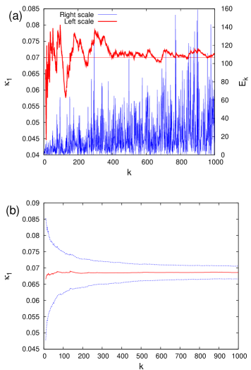
Figure 1: (color online) (a) Time-series of avalanche energies $E_{k}$ (thin blue line, right scale) obtained from Eq.(10) using exponentially distributed $E_{k}$ together with the corresponding evolution of $\kappa_{1}$ (thick red line, left scale) as a function of the number of avalanches $k$. (b)The average value (solid red) and the $\pm\sigma$ intervals (dotted blue) of $\kappa_{1}$ as they result from Monte Carlo calculation of $10^{3}$ realizations of the processes shown in (a).

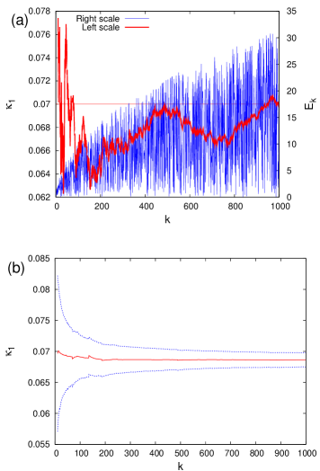
Figure 2: (color online) (a) Time-series of avalanche energies $E_{k}$ (thin blue line, right scale) obtained from Eq.(10) using uniformly distributed $E_{k}$ together with the corresponding evolution of $\kappa_{1}$ (thick red line, left scale) as a function of the number of avalanches $k$. (b)The average value (solid red) and the $\pm\sigma$ intervals (dotted blue) of $\kappa_{1}$ as they result from Monte Carlo calculation of $10^{3}$ realizations of the processes shown in (a).

Figure 1(a) shows with the thin blue line how an example time-series of $E_{k}$, obtained from Eq.(11) for $r_{k}$ exponentially distributed, is read in natural time. It exhibits an intermittent behavior similar to that of Figs.2(a) and 16(c) of Ref. Bonamy (2009), which depict the energy emission versus conventional time from earthquakes and propagating cracks, respectively. In the same figure, we also plot the corresponding $\kappa_{1}$-value as a function of the order $k$ of the avalanche (thick red solid line). Figure 1(b) depicts the average value of $\kappa_{1}$ (red solid line) together with the $\pm\sigma$ (one standard deviation) intervals (blue dotted lines), obtained from the Monte Carlo calculation of the process, an example of which is shown in Fig.1(a). We observe that these $\kappa_{1}$ values scatter around approximately 0.07, while the average value saturates to 0.0686, as expected from the analytical result of the previous Section.

Two additional monoparametric distributions of $E_{k}$ have been also investigated: (a)uniformly distributed $E_{k}$ satisfying Eq.(10), see Fig.2, and (b)Poisson distributed random variables $E_{k}$ obeying Eq.(10), see Fig.3. In addition, we note that when the quantities $r_{k}$, defined in Eq.(11), are Poisson distributed with a mean value $\mu=\langle r_{k}\rangle$, a behavior intermediate between the ones depicted in Figs.1 and 3 -depending on whether $\mu$ is small (with respect to unity) or large, respectively- is found.

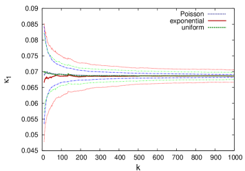
Figure 4: (color online) The average value (dark colors) and the $\pm\sigma$ intervals (light colors) of $\kappa_{1}$ as they result from Monte Carlo calculation of $10^{3}$ realizations for exponentially (red), uniformly (green) and Poisson (blue) distributed $E_{k}$ that satisfy Eq.(10).

The results of the aforementioned three monoparametric distributions investigated, are summarized in Fig. 4. In all cases, the mean value of $\kappa_{1}$ is around 0.070 and tends to the value $\kappa_{1}=0.0686$ obtained analytically from Eq.(9). Among the three monoparametric distributions studied, the exponential exhibits the highest variability while Poisson the smallest. For example at $k=200$ the variability, i.e., the ratio of the standard deviation over the mean value of $\kappa_{1}$ is 6%, 4% and 2% for the exponentially, uniformly and Poisson distributed $E_{k}$, respectively. The latter is understood from the following fact: as the average value $\langle E_{k}\rangle\propto\sqrt{k}$ increases, the Poisson distribution becomes almost Gaussian with standard deviation equal to $\sqrt{\langle E_{k}\rangle}$ which is well localized resulting in a small variability of $\kappa_{1}$ (see also Fig.3(a)). Future research is needed to clarify which of these three distribution is closer to the reality.

V DISCUSSION

In view of the fluctuations seen in Figs.1(a), 2(a), and 3(a), we now study the stability of $\kappa_{1}$ when only one realization of the process is available, as in the case of seismicity (see Appendix). Such a stability is worthwhile to be investigated since it may exist possibly stemming from the following two facts: (a)$\kappa_{1}$ exhibitsVarotsos et al. (2005b) experimental (or LescheLesche (1982, 2004)) stability and (b)Equation (10) has a scale invariant feature.

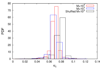
Figure 5: (color online) The probability density functions (PDF) of $\kappa_{1}$ obtained after randomly selecting $M=10^{3}$ (blue) or $M=10^{4}$(red) subseries from a single realization of the process described by Eq.(10) using exponentially distributed $E_{k}$. Both distributions are peaked close to 0.070. Once the events of the original realization are shuffled randomly and then $M=10^{3}$ subseries are analyzed, the peak of the new PDF, shown in black, is displaced to the right.

Exponentially distributed $E_{k}$ satisfying Eq.(10) exhibit, as mentioned, the highest variability, e.g. 6% at $k=200$ (see Figs.1 and 4). Thus, hereafter, we adopt this distribution for the purpose of our study. Focusing on the case of seismicity, after a SES activity and before a mainshock, the following question naturally arises: Since only one realization of the process is known and in view of the variability of $\kappa_{1}$ (see Fig.1), could it be possible to draw any conclusion on the basis of $\kappa_{1}$? The following aspects may answer this question: Let us consider a single realization of Eq.(10) with exponentially distributed $E_{k}$, so that to obtain a series $E_{k}=\epsilon_{k},k=1,2,\ldots,N$. We randomly select a large number $M$ of subseries of $\epsilon_{k}$ of random length $\nu$, which are analyzed in natural time to obtain $\kappa_{1}$. These $\kappa_{1}$-values enable the construction of the probability density function (PDF) of $\kappa_{1}$. For example, let $\nu=3$, and select the subseries $\epsilon_{k_{1}}$, $\epsilon_{k_{2}}$ and $\epsilon_{k_{3}}$, according to their time order, i.e, $k_{1}<k_{2}<k_{3}$. We can then find the corresponding $\kappa_{1}\left[=\sum_{k=1}^{3}\chi_{k}^{2}p_{k}-\left(\sum_{k=1}^{3}\chi_{k}p_{k}\right)^{2}\right]$ value by assuming only three events $k=1,2$ and 3, with $\chi_{1}=1/3$ and $p_{1}=\epsilon_{k_{1}}/(\epsilon_{k_{1}}+\epsilon_{k_{2}}+\epsilon_{k_{3}})$, $\chi_{2}=2/3$ and $p_{2}=\epsilon_{k_{2}}/(\epsilon_{k_{1}}+\epsilon_{k_{2}}+\epsilon_{k_{3}})$ and $\chi_{3}=1$ and $p_{3}=\epsilon_{k_{3}}/(\epsilon_{k_{1}}+\epsilon_{k_{2}}+\epsilon_{k_{3}})$. Figure 5 depicts the PDFs of $\kappa_{1}$ obtained this way from a single realization $\epsilon_{k}$ of $N=300$ events which are exponentially distributed and satisfy Eq.(10) for two values of $M$ ($10^{3}$ or $10^{4}$) when $\nu$ is uniformly distributed from 2 to 300. We observe that the resulting PDF of $\kappa_{1}$ maximizes when $\kappa_{1}\approx 0.070$, i.e., close to the $\kappa_{1}$-value obtained from Eq.(9) for $\lambda=0.5$. This result stems from the fact that the analysis of the subseries maintains the true time order of events which constitutes the key point of natural time. Attention is drawn to the point that if we destroy the order of the events by randomly shuffling $\epsilon_{k}$ and then apply the same procedure, the resulting PDF shown in black in Fig.5 has its peak displaced towards $\kappa_{u}=1/12\approx$0.0833. The latter is the value of $\kappa_{1}$ corresponding to a “uniform” (u) distribution (as defined in Ref. Varotsos et al. (2003a); Varotsos et al. (2004); Varotsos et al. (2005a), e.g. when all $p_{k}$ are equal or $Q_{k}$ are positive independent and identically distributed random variables of finite variance).

Thus, the aforementioned investigation showed that even when using a single realization of the process described by Eq.(10) with $E_{k}$ exponentially distributed, and select random subseries of the process to be analyzed in natural time, the PDF deduced for $\kappa_{1}$ maximizes at $\kappa_{1}\approx 0.070$. This fact, after recalling the point mentioned in Section 1 that seismicity associated with earthquakes seems to belongBonamy (2009) to case (B) (i.e., the macroscopic crack growth when this propagation is slow enough), sheds light on the usefulness of the natural time analysis of the seismicity before a mainshock. This analysis, that is described in detail in the Appendix, considers the time-series of seismicity above a magnitude threshold $M_{thres}$ that occurs after the initiation of the SES activity (which signifies that the system enters the critical regimeVarotsos and Alexopoulos (1986); Varotsos et al. (1998)) in the area candidateVarotsos and Lazaridou (1991); Uyeda et al. (1999); Varotsos (2005); Varotsos et al. (2006b) to suffer a mainshock. In addition, it considers the subseries corresponding to the seismicity in all possible subareas of the candidate area, which enables the construction of the PDF of the resulting $\kappa_{1}$ values. It is foundSarlis et al. (2008) that this PDF exhibits a maximum at $\kappa_{1}\approx 0.070$ (in agreement with Fig.(5)) when approaching the time of occurrence of the main shock. In other words, we set the natural time zero at the initiation time of the SES activity, and then form time series of seismic events in natural time (for every possible subarea), each time when a small earthquake with $M\geq M_{thres}$ occurred, i.e., when the number of events increases by one. Hence, Eq.(7) cannot be misinterpreted as implying that the average energy of each event is increasing for ever as a square root of the index $k$ of the natural time, thus leading to an obviously unacceptable result according to which we have to expect more and more powerful earthquakes in the future. This equation is applied here only for the small events that precede a main shock by starting (i.,e, $k=0$) upon the initiation of the SES activity until just before the main shock occurrence. This behavior should not change upon considering various magnitude thresholds since the process should be scale invariant (see Appendix).

VI CONCLUSIONS

In summary, we studied in natural time, the macroscopic crack growth within a disordered brittle material when the propagation is slow enough. It exhibits jerky dynamics with sudden jumps and energy release events which are power law distributed with universal exponents. By considering that the crack front is self-affine with Family-Vicsek dynamic scaling, we find that the variance $\kappa_{1}(=\langle\chi^{2}\rangle-\langle\chi\rangle^{2})$ is equal to $\kappa_{1}=0.0686(3)$. This, quite interestingly, almost coincides with the value $\kappa_{1}\approx 0.07$ obtained from the natural time analysis of the seismicity that precedes major earthquakes. This conforms with the current aspectBonamy (2009) that the macroscopic crack growth exhibits similar features with the seismicity associated with earthquakes. In other words, the present result that $\kappa_{1}=0.0686$ for the slow propagation of a macroscopic crack in heterogeneous materials through sudden jumps (reminiscent of stick-slip phenomena), sheds light on the following finding: After the detection of a SES activity (critical dynamics), when following the dynamic evolution of the system by computing $\kappa_{1}$ after each small earthquake -by means of the natural time analysis of seismicity- and find that $\kappa_{1}\approx 0.07$, we identify that the system approached the critical point and the major mainshock occurs.

Appendix A Application of the results obtained from the natural time analysis of macroscopic crack propagation to real seismic data

Here, we focus on the analysis of the seismicity after the initiation of a SES activity and before a mainshock. Once a SES activity has been recorded, which signifies that the system just entered the critical regimeVarotsos and Alexopoulos (1986); Varotsos et al. (1998), an estimation of the area to suffer a mainshock can be obtained on the basis of the so-called selectivity mapVarotsos and Lazaridou (1991); Uyeda et al. (1999); Varotsos (2005); Varotsos et al. (2006b) of the station at which the SES observation was made. Thus, we have some area, hereafter labelled A, in which we count the small events (earthquakes) $e_{i}$ that occur after the initiation of the SES activity. Each event $e_{i}$ is characterized by its location ${\bf x}(e_{i})$, the conventional time of its occurrence $t(e_{i})$, and its magnitude ${\rm M}(e_{i})$ or the equivalent seismic moment $M_{0}(e_{i})$ (e.g. see Ref. Hanks and Kanamori (1979)). The index $i=1,2,\ldots,N$ increases by one each time a new earthquake occurs within the area A (cf. $\forall i,t(e_{i+1})>t(e_{i})$). Thus, a set of events $\cal{A}$ is formed until the mainshock occurs in A at $i=N$. To be more precise, a family of sets ${\cal A}_{{\rm M}_{thres}}$ of the earthquakes with magnitude greater than or equal to $M_{thres}$ is formed, where ${\cal A}_{{\rm M}_{thres}}=\left\{e_{i}\in{\cal A}:{\rm M}(e_{i})\geq{\rm M}_{thres}\right\}$ and the number of events in ${\cal A}_{{\rm M}_{thres}}$ is denoted by $|{\cal A}_{{\rm M}_{thres}}|$. The set ${\cal A}_{{\rm M}_{thres}}$ becomes a (time) ordered set by selecting the indices $j$ for its elements $e_{j}$, $j=1,2,\ldots,|{\cal A}_{{\rm M}_{thres}}|$ so that $\forall j,t(e_{j+1})>t(e_{j})$. Since earthquakes do not occur everywhere within the area A but in some specific locations, we may also define $R({\cal A}_{{\rm M}_{thres}})$ as the minimal rectangular (in latitude and longitude) region in which the epicenters of the events of ${\cal A}_{{\rm M}_{thres}}$ are located. Moreover, for a given ordered set ${\cal A}_{{\rm M}_{thres}}$ the corresponding value of $\kappa_{1}({\cal A}_{{\rm M}_{thres}})$ can be obtained by analyzing in natural time its ordered elements $e_{j}$ ($\in{\cal A}_{{\rm M}_{thres}}$). This is made by analyzing in natural time the pairs $(\chi_{j},Q_{j})=(j/|{\cal A}_{{\rm M}_{thres}}|,M_{0}(e_{j}))$ where $j=1,2,\ldots,|{\cal A}_{{\rm M}_{thres}}|$.

The key point behind this approach, is the experimental (or LescheLesche (1982, 2004)) stability that is satisfiedVarotsos et al. (2005b) by the variance $\kappa_{1}$ in combination with the conclusion drawn in Section 5. We define a proper subset ${\cal P}_{{\rm M}_{thres}}$ of ${\cal A}_{{\rm M}_{thres}}$ as a subset of ${\cal A}_{{\rm M}_{thres}}\left(\supset{\cal P}_{{\rm M}_{thres}}\right)$ such that it includes all the elements of ${\cal A}_{{\rm M}_{thres}}$ that occurred after the SES initiation and before the mainshock in $R({\cal P}_{{\rm M}_{thres}})$. Finally, we consider the ensemble ${\cal E[A}_{{\rm M}_{thres}}]$ of all different ${\cal P}_{{\rm M}_{thres}}$ which one can define from a given ${\cal A}_{{\rm M}_{thres}}$. For each member of this ensemble, we can find the corresponding $\kappa_{1}$ value and, when considering the totality of these values for the ensemble, we can construct the PDF of $\kappa_{1}$. If the earthquakes under consideration belong to a self-similar preparation process, we expect that at the later stages of this process, where Eq.(10) might be valid, the PDF should exhibit a maximum at $\kappa_{1}=0.070$. All the recent experimental results associated with the major earthquakes in Greece (see Ref. Sarlis et al. (2008)) indicate that before the occurrence of a mainshock this PDF (or equivalently the probability Prob($\kappa_{1}$) versus $\kappa_{1}$) exhibits a maximum close to $\kappa_{1}=0.070$, in agreement with Fig.5.

As an example, we summarize here the results obtained for the case of the $M_{w}$6.4 earthquake that occurred at 38.0^oN21.5^oE at 12:25UT on 8 June 2008, which is the latest $M_{w}>6.0$ earthquake in Greece. Figure 7(c) of Ref. Sarlis et al. (29 May 2008)(or Fig.3(b) of Ref. Sarlis et al. (2008)) depicts a long duration SES activity that was recorded at Pirgos (Greece) measuring station from 29 February 2008 to 2 March 2008. This SES activity, as shown in Ref. Varotsos et al. (2009), exhibits self-similar structure over five orders of magnitude with a (self-similarity) exponent close to unity. By studying the seismicity, after the initiation of this SES activity in the grey shaded area of Fig.8 of Ref. Sarlis et al. (29 May 2008) (or Ref. Sarlis et al. (2008)), which constitutes the SES selectivity map of Pirgos station, we obtained (just after the occurrence of an earthquake of magnitude 5.1 at 23:26UT on 27 May 2008) the probabilities Prob($\kappa_{1}$) shown in Figs.6(a), (b) and (c) for $M_{thres}=3.9$, 4.0 and 4.1, respectively. These distributions exhibit a maximum at $\kappa_{1}=0.070$ independent of the magnitude threshold (as intuitively expected for a self-similar preparation process). This fact was reportedSarlis et al. (29 May 2008) on 29 May 2008, and eleven days later the aforementioned $M_{w}$6.4 mainshock occurred within the area (selectivity map of Pirgos station) specified in advance (cf. such predictions are issued only when the expected magnitude of the impending mainshock is 6.0 or larger, e.g., see Ref.Varotsos (2005)).

Note added on December 8, 2017: An SES activity with properties different from those of the previous SES activity at ASS reported in Ref.note was recorded at ASS station on 23 November 2017 and is depicted in Fig.8. The upper 3 channels correspond to the three components of the magnetic field measured by DANSK coil magnetometers and the other 13 channels to electric field variations measured by several short- and long-dipoles of length lying between 100 m and $\approx$9.6 km. The subsequent seismicity in the ASS selectivity map shown by the red dashed dotted line in Fig.7 is currently analyzed in natural time in order to identify the occurrence time of the impending mainshock.

Note added on February 14, 2018: Actually on 2 January 2018 an earthquake of magnitude ML(ATH)4.7, i.e., Ms(ATH)5.2, occurred with an epicenter at 41.2^oN, 22.9^oE lying within the shaded region “c” of the SES selectivity map of ASS, shown in Fig.7, at a distance of a few tens of km from the measuring station. Subsequently, the continuation of the natural time analysis of seismicity after the SES activity (Fig.8) recorded at ASS revealed that on 13 February 2018 upon the occurrence of a number of seismic events within the shaded region “a” as well as in the vicinity of the shaded region “b” the PDF Prob($\kappa_{1}$) versus $\kappa_{1}$ shows a feature (in a similar fashion as Fig.7.23 of Ref.Varotsos et al. (2011a)) one mode of which maximizes at $\kappa_{1}=0.070$ exhibiting magnitude threshold invariance (cf. four such examples are depicted for $M_{thres}$=2.6, 2.7, 2.8 and 2.9 in Fig.9).

Note added on June 26, 2018: On 24 April 2018 and 25 April 2018 two SES activites have been recorded again at ASS (see Fig.10(a),(b)) but with opposite polarity than the SES activity in Fig.8. We recall that an SES activity initiates when a minimum $\beta_{\rm min}$ of the order parameter of seismicity is observed and in addition it has been found [N. Sarlis et al. Proc. Natl. Acad. Sci. U.S.A. 110 (2013), 13734-13738] that all major shallow earthquakes in Japan were preceded by minima $\beta_{\rm min}$ with lead times around two to three months.

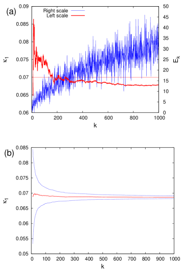
Figure 3: (color online) (a) Time-series of avalanche energies $E_{k}$ (thin blue line, right scale) obtained from Eq.(10) using Poisson distributed $E_{k}$ together with the corresponding evolution of $\kappa_{1}$ (thick red line, left scale) as a function of the number of avalanches $k$. (b)The average value (solid red) and the $\pm\sigma$ intervals (dotted blue) of $\kappa_{1}$ as they result from Monte Carlo calculation of $10^{3}$ realizations of the processes shown in (a).

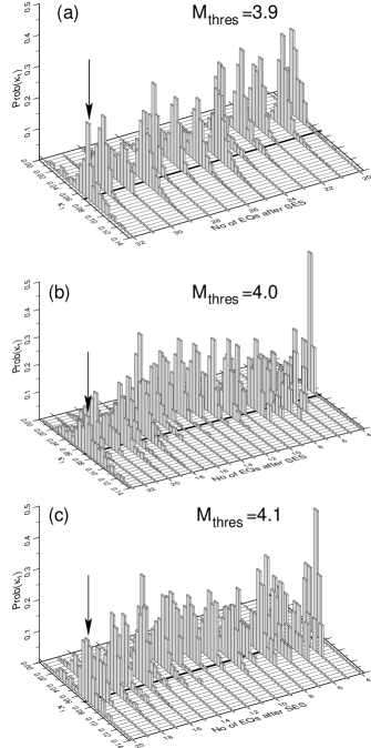
Figure 6: (a):Prob($\kappa_{1}$) versus $\kappa_{1}$ of the seismicity(subsequent to the long duration SES activity recorded at Pirgos station during February 29 to March 2, 2008), for $M_{thres}=3.9$, within the SES selectivity map of Pirgos station (which is the shaded area shown in Fig.8 of Ref. Sarlis et al. (29 May 2008)). The arrow marks the maximum of Prob($\kappa_{1}$) at $\kappa_{1}=0.07$ that occurred on 27 May 2008 (i.e., upon the occurrence of the 32nd event after the SES). This maximum has been followed by the $M_{w}$6.4 mainshock on 8 June 2008. (b) and (c) are the same as (a), but for $M_{thres}=4.0$ and $M_{thres}=4.1$, respectively. The arrows in (b) and (c) indicate the maximum of Prob($\kappa_{1}$) at $\kappa_{1}\approx 0.070$ that also occurred on 27 May 2008.

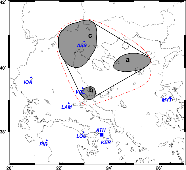
Figure 7: Map showing the operating VAN stations (blue triangles). The ASS selectivity map is bounded by the red dashed-dotted line as it was obtained in N. Sarlis, Proc. Jpn. Acad. Ser. B 89, 438-445 (2013).

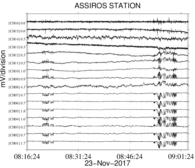
Figure 8: The SES activity recorded at ASS station on 23 November 2017. The upper three channels (i.e., CH14, CH15 and CH16) correspond to magnetic field changes recorded by coil magnetometers while the channels labeled CH01 to CH13 to electric field changes (see the text).

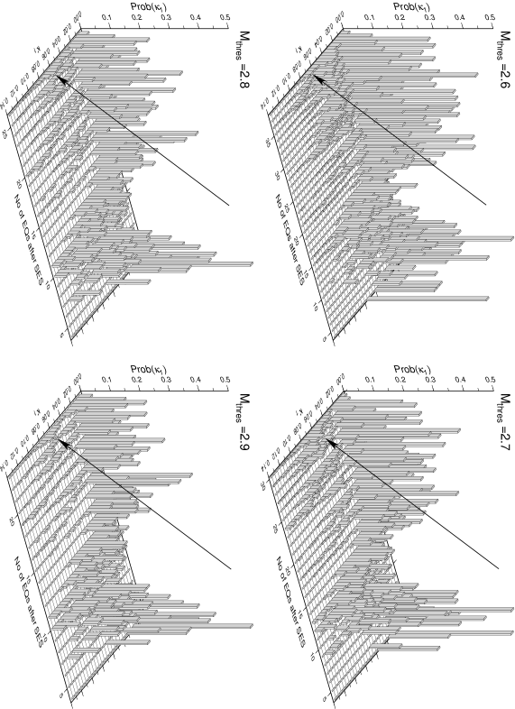
Figure 9: Prob($\kappa_{1}$) versus $\kappa_{1}$ of the seismicity(subsequent to the SES activity recorded at ASS station depicted in Fig.8) for $M_{thres}$=2.6, 2.7, 2.8 and 2.9, within the SES selectivity map of ASS station shown in Fig.7. The arrows mark the mode of Prob($\kappa_{1}$) that maximizes at $\kappa_{1}=0.07$ that occurred on 13 February 2018.

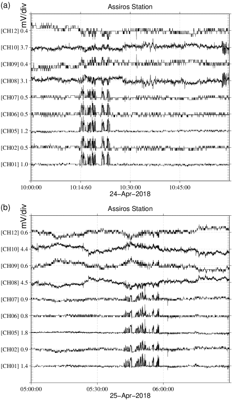
Figure 10: The two SES activities recorded at ASS station on 24 April 2018 (a) and 25 April 2018 (b). The ASS selectivity map is shown in Fig.7.

References

- Alava et al. (2006) M. J. Alava, P. K. V. V. Nukala, and S. Zapperi, Adv. Phys. 55, 349 (2006).
- Bonamy et al. (2008) D. Bonamy, S. Santucci, and L. Ponson, Phys. Rev. Lett. 101, 045501 (2008).
- Bouchaud and Soukiassian (2009) E. Bouchaud and P. Soukiassian, Journal of Physics D: Applied Physics 42, 210 (2009).
- Bonamy (2009) D. Bonamy, J. Phys. D: Appl. Phys. 42, 214014 (2009).
- Bouchaud (1997) E. Bouchaud, Journal of Physics: Condensed Matter 9, 4319 (1997).
- Bonamy et al. (2006) D. Bonamy, L. Ponson, S. Prades, E. Bouchaud, and C. Guillot, Phys. Rev. Lett. 97, 135504 (2006).
- Måløy and Schmittbuhl (2001) K. J. Måløy and J. Schmittbuhl, Phys. Rev. Lett. 87, 105502 (2001).
- Santucci et al. (2004) S. Santucci, L. Vanel, and S. Ciliberto, Phys. Rev. Lett. 93, 095505 (2004).
- Marchenko et al. (2006) A. Marchenko, D. Fichou, D. Bonamy, and E. Bouchaud, Appl. Phys. Lett. 89, 093124 (2006).
- Sethna et al. (2001) J. P. Sethna, K. A. Dahmen, and C. R. Myers, Nature (London) 410, 242 (2001).
- Garcimartín et al. (1997) A. Garcimartín, A. Guarino, L. Bellon, and S. Ciliberto, Phys. Rev. Lett. 79, 3202 (1997).
- Davidsen et al. (2007) J. Davidsen, S. Stanchits, and G. Dresen, Phys. Rev. Lett. 98, 125502 (2007).
- Family and Vicsek (1991) F. Family and T. Vicsek, eds., Dynamics of Fractal Surfaces (World Scientific, Singapore, 1991).
- Måløy et al. (2006) K. J. Måløy, S. Santucci, J. Schmittbuhl, and R. Toussaint, Phys. Rev. Lett. 96, 045501 (2006).
- Ponson (2009) L. Ponson, Phys. Rev. Lett. 103, 055501 (2009).
- Koivisto et al. (2007) J. Koivisto, J. Rosti, and M. J. Alava, Phys. Rev. Lett. 99, 145504 (2007).
- Griffith (1921) A. A. Griffith, Phil. Trans. R. Soc. Lond. A 221, 163 (1921).
- Gao and Rice (1986) H. Gao and J. R. Rice, J. Appl. Mech. 53, 774 (1986).
- Wert and Zener (1949) C. Wert and C. Zener, Phys. Rev. 76, 1169 (1949).
- Zener (1951) C. Zener, Journal of Applied Physics 22, 372 (1951).
- Kostopoulos et al. (1975) D. Kostopoulos, P. Varotsos, and S. Mourikis, Can. J. Phys. 53, 1318 (1975).
- Varotsos and Alexopoulos (1977) P. Varotsos and K. Alexopoulos, J Phys. Chem. Solids 38, 997 (1977).
- Varotsos et al. (1982) P. Varotsos, K. Alexopoulos, and K. Nomicos, Phys. Status Solidi B 111, 581 (1982).
- Varotsos and Alexopoulos (1982) P. Varotsos and K. Alexopoulos, physica status solidi (b) 110, 9 (1982).
- Varotsos (1980) P. Varotsos, physica status solidi (b) 100, K133 (1980).
- Varotsos and Alexopoulos (1978) P. Varotsos and K. Alexopoulos, Phys. Status Solidi A 47, K133 (1978).
- Varotsos (2008) P. Varotsos, Solid State Ionics 179, 438 (2008).
- Schmittbuhl et al. (1995) J. Schmittbuhl, S. Roux, J.-P. Vilotte, and K. Jorgen Måløy, Phys. Rev. Lett. 74, 1787 (1995).
- Ramanathan et al. (1997) S. Ramanathan, D. Erta, and D. S. Fisher, Phys. Rev. Lett. 79, 873 (1997).
- Varotsos (2005) P. Varotsos, The Physics of Seismic Electric Signals (TERRAPUB, Tokyo, 2005).
- Bak et al. (1987) P. Bak, C. Tang, and K. Wiesenfeld, Phys. Rev. Lett. 59, 381 (1987).
- Varotsos et al. (2002a) P. A. Varotsos, N. V. Sarlis, and E. S. Skordas, Phys. Rev. E 66, 011902 (2002a).
- Varotsos et al. (2003a) P. A. Varotsos, N. V. Sarlis, and E. S. Skordas, Phys. Rev. E 67, 021109 (2003a).
- Varotsos et al. (2004) P. A. Varotsos, N. V. Sarlis, E. S. Skordas, and M. S. Lazaridou, Phys. Rev. E 70, 011106 (2004).
- Varotsos et al. (2005a) P. A. Varotsos, N. V. Sarlis, E. S. Skordas, and M. S. Lazaridou, Phys. Rev. E 71, 011110 (2005a).
- Varotsos et al. (2005b) P. A. Varotsos, N. V. Sarlis, H. K. Tanaka, and E. S. Skordas, Phys. Rev. E 71, 032102 (2005b).
- Varotsos et al. (2005c) P. A. Varotsos, N. V. Sarlis, H. K. Tanaka, and E. S. Skordas, Phys. Rev. E 72, 041103 (2005c).
- Varotsos et al. (2006a) P. A. Varotsos, N. V. Sarlis, E. S. Skordas, H. K. Tanaka, and M. S. Lazaridou, Phys. Rev. E 73, 031114 (2006a).
- Varotsos et al. (2008) P. A. Varotsos, N. V. Sarlis, E. S. Skordas, and M. S. Lazaridou, J. Appl. Phys. 103, 014906 (2008).
- Sarlis et al. (2009a) N. V. Sarlis, E. S. Skordas, and P. A. Varotsos, Phys. Rev. E 80, 022102 (2009a).
- Sarlis et al. (2008) N. V. Sarlis, E. S. Skordas, M. S. Lazaridou, and P. A. Varotsos, Proc. Jpn. Acad., Ser. B: Phys. Biol. Sci. 84, 331 (2008).
- Varotsos et al. (2009) P. A. Varotsos, N. V. Sarlis, and E. S. Skordas, Chaos: An Interdisciplinary Journal of Nonlinear Science 19, 023114 (2009).
- Varotsos et al. (2007) P. A. Varotsos, N. V. Sarlis, E. S. Skordas, and M. S. Lazaridou, Appl. Phys. Lett. 91, 064106 (2007).
- Sarlis et al. (2009b) N. V. Sarlis, E. S. Skordas, and P. A. Varotsos, EPL 87, 18003 (2009b), URL http://dx.doi.org/10.1209/0295-5075/87/18003.
- Sarlis et al. (2006) N. V. Sarlis, P. A. Varotsos, and E. S. Skordas, Phys. Rev. B 73, 054504 (2006).
- Wigner (1932) E. Wigner, Phys. Rev. 40, 749 (1932).
- Tsallis (1988) C. Tsallis, J. Stat. Phys. 52, 479 (1988).
- Abe et al. (2005) S. Abe, N. V. Sarlis, E. S. Skordas, H. K. Tanaka, and P. A. Varotsos, Phys. Rev. Lett. 94, 170601 (2005).
- Cohen (1994) L. Cohen, Time-Frequency Analysis. Theory and Applications (Prentice-Hall, Upper Saddle river, NJ, 1994).
- Grob et al. (2009) M. Grob, J. Schmittbuhl, R. Toussaint, L. Rivera, S. Santucci, and K. J. Måløy, Pure and Applied Geophysics 166, 777 (2009).
- Uyeda et al. (2009) S. Uyeda, M. Kamogawa, and H. Tanaka, J. Geophys. Res. 114, B02310, doi:10.1029/2007JB005332 (2009).
- Uyeda and Kamogawa (2008) S. Uyeda and M. Kamogawa, Eos Trans. AGU 89, 363 (2008).
- Uyeda and Kamogawa (2010) S. Uyeda and M. Kamogawa, Eos Trans. AGU 91, 163 (2010).
- Varotsos et al. (1996) P. Varotsos, K. Eftaxias, M. Lazaridou, K. Nomicos, N. Sarlis, N. Bogris, J. Makris, G. Antonopoulos, and J. Kopanas, Acta Geophysica Polonica 44, 301 (1996).
- Varotsos et al. (2002b) P. A. Varotsos, N. V. Sarlis, and E. S. Skordas, Acta Geophysica Polonica 50, 337 (2002b).
- Varotsos et al. (2013) P. A. Varotsos, N. V. Sarlis, E. S. Skordas, and M. S. Lazaridou, Tectonophysics 589, 116 (2013).
- Varotsos et al. (1993) P. Varotsos, K. Alexopoulos, M. Lazaridou-Varotsou, and T. Nagao, Tectonophysics 224, 269 (1993).
- Varotsos et al. (2011) P. Varotsos, N. V. Sarlis, E. S. Skordas, S. Uyeda, and M. Kamogawa, Proc. Natl. Acad. Sci. USA 108, 11361 (2011).
- Varotsos and Alexopoulos (1986) P. Varotsos and K. Alexopoulos, Thermodynamics of Point Defects and their Relation with Bulk Properties (North Holland, Amsterdam, 1986).
- Varotsos et al. (1998) P. Varotsos, N. Sarlis, M. Lazaridou, and P. Kapiris, J. Appl. Phys. 83, 60 (1998).
- Varotsos et al. (2001) P. Varotsos, N. Sarlis, and E. Skordas, Proc. Jpn. Acad., Ser. B: Phys. Biol. Sci. 77, 87 (2001).
- Varotsos et al. (2003b) P. A. Varotsos, N. V. Sarlis, and E. S. Skordas, Phys. Rev. Lett. 91, 148501 (2003b).
- Hanks and Kanamori (1979) T. C. Hanks and H. Kanamori, J. Geophys. Res. 84(B5), 2348 (1979).
- Feller (1971) W. Feller, An Introduction to Probability Theory and Its Applications, Vol. II (Wiley, New York, 1971).
- Rosso and Krauth (2002) A. Rosso and W. Krauth, Phys. Rev. E 65, 25101 (2002).
- Duemmer and Krauth (2007) O. Duemmer and W. Krauth, J. Stat. Mech. 1, P01019, doi:10.1088/1742 (2007).
- Lesche (1982) B. Lesche, J. Stat. Phys. 27, 419 (1982).
- Lesche (2004) B. Lesche, Phys. Rev. E 70, 017102 (2004).
- Varotsos and Lazaridou (1991) P. Varotsos and M. Lazaridou, Tectonophysics 188, 321 (1991).
- Uyeda et al. (1999) S. Uyeda, E. Al-Damegh, E. Dologlou, and T. Nagao, Tectonophysics 304, 41 (1999).
- Varotsos et al. (2006b) P. Varotsos, N. Sarlis, S. Skordas, and M. Lazaridou, Tectonophysics 412, 279 (2006b).
- Sarlis et al. (29 May 2008) N. V. Sarlis, E. S. Skordas, M. S. Lazaridou, and P. A. Varotsos (29 May 2008), arXiv:0802.3329v4.
- (73) Note added on May 4, 2017: An SES activity was recorded at ASS station (lying close to Thessaloniki) on April 18, 2017, at 07:50 UT. In order to determine the occurrence time of the impending mainshock, immediately after the initiation of this SES activity, we started an analysis in natural time of the seismicity occuring within the ASS selectivilty map shown by the red dashed-dotted line in Fig.7.
- Varotsos et al. (2011a) P. A. Varotsos, N. V. Sarlis, and E. S. Skordas, Natural Time Analysis: The new view of time. Precursory Seismic Electric Signals, Earthquakes and other Complex Time-Series (Springer-Verlag, Berlin Heidelberg, 2011a).