Estimating the sensitivity of centrality measures w.r.t. measurement errors

Abstract

Most network studies rely on an observed network that differs from the underlying network which is obfuscated by measurement errors. It is well known that such errors can have a severe impact on the reliability of network metrics, especially on centrality measures: a more central node in the observed network might be less central in the underlying network.

We introduce a metric for the reliability of centrality measures – called sensitivity. Given two randomly chosen nodes, the sensitivity means the probability that the more central node in the observed network is also more central in the underlying network. The sensitivity concept relies on the underlying network which is usually not accessible. Therefore, we propose two methods to approximate the sensitivity. The iterative method, which simulates possible underlying networks for the estimation and the imputation method, which uses the sensitivity of the observed network for the estimation. Both methods rely on the observed network and assumptions about the underlying type of measurement error (e.g., the percentage of missing edges or nodes).

Our experiments on real-world networks and random graphs show that the iterative method performs well in many cases. In contrast, the imputation method does not yield useful estimations for networks other than Erdős–Rényi graphs.

1 Introduction

Measurement errors in network data are a central problem in the field of network analysis. Virtually all empirical network data is affected by a certain kind of measurement error and previous research has shown that these errors often have a major impact on the results of network analysis methods, especially on centrality measures  [36]. For example, a more central node in the observed (erroneous) network might be less central in the hidden (unobserved, error-free) network. To quantify the impact of measurement errors on centrality measures, we introduce a metric – called sensitivity. Given two randomly chosen nodes, the sensitivity means the probability that the more central node in the observed network is also more central in the underlying network.

Currently, most applied network studies only report that measurement errors might have affected the data collection (e.g., due to absence of actors at the day of the survey or due to the study design). Most of the time, however, the impact of these measurement errors on centrality measures are not discussed. This might be due to the fact that there is currently no established way to estimate the sensitivity for an observed network.

Some researchers have investigated the impact that different kinds of measurement errors have on the reliability of centrality measures in the case of random graphs and real-world networks [9, 6, 21, 12, 36, 33, 29, 28, 24]. For an extensive survey of previous studies about the reliability of centrality measures see Smith et al. (2017) [34]. These important studies provide guidelines for researchers on how to design future studies (e.g., what kind of measurement error might be especially harmful in a given scenario) and suggestions on which centrality measure might be more reliable in a given scenario. Unfortunately, it is difficult to identify general patterns for the reliability of centrality measures in real-world networks. As common sense suggests, centrality measures become less reliable with an increasing level of error. Additionally, the particular relationship between error level and reliability is highly dependent on the type of measurement error, the centrality measure, and the network structure.

There are studies that use the observed network to reconstruct the hidden network, estimate statistics about the hidden network, or estimate the influence that measurement errors have on network analysis methods [8, 18, 16, 20, 11, 35, 27]. Despite their important contributions, these studies usually focus on network invariants (e.g., diameter or average path length) and do not explicitly address node invariants (e.g., the centrality values for all nodes in a network).

Studies about the robustness of networks, the capacity of networks to maintain functionality when the network is modified, also usually focus on network invariants. In this paper, however, we do not study the robustness of networks. For an extensive overview about the robustness of networks see Barabási (2016) [2] and Havlin & Cohen (2010) [17].

The sensitivity concept relies on the hidden network which is usually not accessible. In this paper, we propose two methods (“imputation method” and “iterative method”) that allow the researcher to estimate the sensitivity of the hidden network, given the observed network and some assumptions about the measurement error. In case of the imputation method, we try to simulate the hidden network by inverting the measurement error (e.g.: if 10% of randomly chosen edges are missing, we add 11,11% edges by linking randomly chosen pairs of non-adjacent nodes) and then compute the sensitivity with respect to the simulated hidden network. In case of the iterative method, we assume that the considered hidden network has a certain kind of self-similarity property. That is, we assume that the sensitivity of the observed network (regarding the assumed measurement error) is a good estimate of the sensitivity of the hidden network. While it is known that imputation techniques may work well [30, 1, 31], simulating appropriate hidden networks is complicated and calculating the estimate based on the imputation method is, therefore, difficult. In contrast, the estimate based on the iterative method is relatively easy to calculate. However, this method relies on a self-similarity property that is difficult to verify. In addition to the estimation methods, we introduce an easy-to-interpret measure for the reliability of centrality measures and a generic concept to model measurement errors. We test both estimation methods on random graphs and real-world networks. While the imputation method and the iterative method perform well on Erdős–Rényi graphs (ER graphs), the iterative method, which is easier to calculate, performs much better in case of Barabási–Albert graphs (BA graphs) and real-world networks. For real-world networks, the iterative method performs especially well in case of the PageRank. To measure the reliability of centrality measures, we introduce the necessary concepts in Section 2. The estimation methods are presented in Section 3. In Section 4, we apply these methods to real-world networks. Results are discussed in Section 5.

2 Basic concepts

Let G be an undirected, unweighted, finite graph with vertex set $V(G)$ and edge set $E(G)$. A centrality measure $c$ is a real-valued function that assigns centrality values to all nodes in a graph and is invariant to structure-preserving mappings, i.e., centrality values depend solely on the structure of a graph. External information (e.g., node or edge attributes) have no influence on the centrality values (cf. Koschützki et al. (2005) [22]). We denote the centrality value for node $u\in V(G)$ by $c_{G}(u)$ and the centrality values for all nodes in G $(u_{1},u_{2},\dots,u_{n})$ by the vector $c(G):=(c(u_{1}),\dots,c(u_{n}))$.

The following centrality measures are used in this study: closeness centrality, betweenness centrality [13], degree centrality, eigenvector centrality [5], and the PageRank [7]. All centrality measures are calculated using the igraph library (version 0.7.1, Csardi & Nepusz [10]).

Let G and $G^{\prime}$ be two graphs and $c$ a centrality measure. A pair of nodes $u,v\in V(G)\cap V(G^{\prime})$ and $u\neq v$ is called concordant w.r.t. $c$ if both nodes have distinct centrality values and the order of u and v is the same in c(G) and c($G^{\prime}$), i.e., either $c_{G}(u)<c_{G}(v)$ and $c_{G^{\prime}}(u)<c_{G^{\prime}}(v)$ or $c_{G}(u)>c_{G}(v)$ and $c_{G^{\prime}}(u)>c_{G^{\prime}}(v)$. A pair of nodes is called discordant if both nodes have distinct centrality values and the order of u and v in c(G) differs from the order of u and v in c($G^{\prime}$), i.e., either $c_{G}(u)<c_{G}(v)$ and $c_{G^{\prime}}(u)>c_{G^{\prime}}(v)$ or $c_{G}(u)>c_{G}(v)$ and $c_{G^{\prime}}(u)<c_{G^{\prime}}(v)$. Ties are neither concordant nor discordant.

A random graph consists of a finite set of graphs $\Omega$ equipped with a function $P$ that assigns a probability to every graph in this set (cf. Bollobás & Riordan (2002) [4]).

2.1 Modeling measurement errors

Network data can be influenced by a variety of different measurement errors. Recently, Wang et al. [36] categorized measurement errors into six groups: false negative nodes and edges, false positive nodes and edges, and false aggregation and disaggregation. For example, when 10% of the edges are missing in the observed network data, the graph constructed from this observed data suffers from false negative edges.

To describe measurement errors, we introduce the notion of an error mechanism. An error mechanism $\varphi$ is a procedure that describes measurement errors which may occur during the data collection. For a graph G, $\varphi(G)$ is a random graph which probability distribution for the possible graphs depends on the error procedure that describes $\varphi$. Hence, all graphs that could be observed when the error procedure influences the data collections are possible outcomes of this random graph.

To illustrate the concept of an error mechanism, consider the graphs illustrated in Figure 1. The initial graph is denoted by H (drawn in the upper left corner). We assume that we know the error mechanism that compromises the data collection. For this example, we assume that the error mechanism $\varphi$ is edges missing uniformly at random with an error level of 50%. All graphs in the set of possible outcomes for this random graph $\Omega=\{G_{1},G_{2},\dots,G_{6}\}$ are also shown in Figure 1. In this example, the probability function is $P(G_{i})=\frac{1}{6}$; all graphs in $\Omega$ occur with the same probability. However, this concept is not limited to a uniform distribution.

Figure 1: In this example, $\varphi$ is defined as the error mechanism “50% of all edges are missing uniformly at random”. Hence, $\varphi(H)$ is a random graph with possible outcomes $\Omega=\{G_{1},G_{2},\dots,G_{6}\}$ and $P(G_{i})=\frac{1}{6}$.

In general, error mechanisms can rely on node or edge attributes. In this study, we focus on four common error mechanism that do not depend on external attributes:

1. Nodes missing uniformly at random (rm nodes): A fraction of nodes (and all edges connected to these nodes) is missing in the observed network. All nodes have the same probability to be missing in the observed network.

2. Edges missing uniformly at random (rm edges unif.): A fraction of edges is missing in the observed network. All edges have the same probability to be missing in the observed network.

3. Edges missing proportional (rm edges prop.): A fraction of edges is missing in the observed network. The probability that an edge is missing in the observed network is proportional to the sum of the degree values of the endpoints.

4. Spurious edges (add edges): The observed network contains too many edges. Every non-existing edge has the same probability to be erroneously observed.

Imputation techniques are commonly used to replace missing data with plausible estimates. Inspired by Huisman [18], we define an imputation mechanism as a procedure that aims to ‘undo’ the effects that measurement errors have on network data.

For a given error scenario, there might be multiple or no appropriate imputation mechanisms. Moreover, the choice of the appropriate imputation mechanism depends on the type of measurement error and possibly also on the network structure. For example, if edges are missing uniformly at random, a possible imputation mechanism is to add edges randomly (uniform) to the observed network. However, the success of this procedure depends on the structure of the network. Consider the scenario that the hidden network is a star graph. In this case, it is quite likely that this imputation approach would have a negative impact on subsequent analyses because it is much more likely that the imputed edges are between leaf nodes than between the internal node and a leaf node. Hence, if the structure of the hidden network is not known (which is usually the case), it is difficult to define an appropriate imputation procedure.

We use $\psi$ to denote a specific imputation mechanism. Analogously to error mechanisms, $\psi(G)$ denotes a random graph. All graphs that can occur when the imputation mechanism $\psi$ is applied to graph $G$ are possible outcomes for this random graph. In this paper, we use three generic imputation mechanisms:

1. If $k$ edges are missing in the observed network, we choose $k$ edges uniformly at random from the set of edges that are not in the observed network and add them to the observed network.

2. If there are $k$ spurious edges in the observed network, we choose $k$ edges that do exist in the observed network and delete them.

3. If $k$ nodes are missing, we choose the degrees for $k$ new nodes from the current degree distribution and successively add these nodes to the networks. The links between new and existing nodes are created uniformly at random.

2.2 Sensitivity of centrality measures

Let G and $G^{\prime}$ denote graphs on the same vertex set and $c$ a centrality measure. The sensitivity of the centrality measure $c$ w.r.t. those two graphs is the probability that two nodes with distinct centrality values, randomly chosen from the vertex set of G and $G^{\prime}$, have the same order in c(G) and c($G^{\prime}$), i.e., they are concordant. If this quantity is close to one, the centrality measure is considered to be robust. If it is close to zero, the centrality measure is considered to be sensitive. We calculate the sensitivity $\rho$ for a centrality measure $c$ with respect to G and $G^{\prime}$ as follows:

$$\rho_{c}(G,{G^{\prime}})=\frac{n_{c}}{n_{c}+n_{d}}$$ (1)

With $n_{c}$ as the number of concordant pairs and $n_{d}$ as the number of discordant pairs w.r.t. the order given by $c(G)$ and $c({G^{\prime}})$.

The sensitivity as defined above is closely related to Goodman and Kruskal’s rank correlation coefficient $\gamma$ which is the difference between concordant and discordant pairs divided by the sum of concordant and discordant pairs [15]. We can use this relationship to calculate the sensitivity as follows:

$$\rho_{c}(G,{G^{\prime}})=\frac{\gamma(c(G),c({G^{\prime}}))+1}{2}.$$ (2)

Let us apply this concept to a graph illustrated in Figure 1. Assume that we have observed the graph labeled as $G_{6}$ and that we are interested in the sensitivity of the degree centrality. Then, the degree centrality values are $deg(H)=(1,2,3,1,1)$ and $deg(G_{6})=(1,2,1,0,0)$. Based on the degree values, we can calculate the sensitivity of the degree centrality with respect to $G_{6}$ and H: $\rho_{deg}(G_{6},H)=\frac{5}{6}$. If we randomly choose a pair of nodes, there is a 0.83 chance that their order induced by the degree centrality is the same in both graphs.

2.3 Exemplary application of the sensitivity concept

In this section, we apply the concepts introduced above to analyze the sensitivity of centrality measures in ER graphs.

For all combinations of centrality measures and error mechanisms introduced in Section 2 and 2.1, we perform the experiment described below 500 times. For every error mechanism, we consider two cases, a moderate scenario of 10% error level and a more intense scenario with 30% error level. The procedure for the experiment is as follows:

1. Generate an ER graph with 100 nodes and edge probability 0.2 and denote it by H. This is the error-free (hidden) graph which is not available to the researcher.

2. Choose a graph from $\varphi(H)$ and denote it by O. This is the observed graph which is affected by measurement errors.

3. Calculate the sensitivity $\rho_{c}(O,H)$.

The results are shown in Figure 2. Every panel shows violin plots for the distribution of the sensitivity of the centrality measures. Despite the fact that these graphs are very homogeneous, we make interesting observations. The sensitivity differs between centrality measures. The degree centrality is, in all cases, the most robust measure. Generally, the sensitivity values for the 30% error mechanisms are much lower than for the 10% error mechanism. The variance of the sensitivity values also increases with increasing error level. Usually, the sensitivity also depends on the error mechanism. However, this is not always the case. (e.g., degree centrality the the case of 10% error mechanisms). These observations are conclusive with the results of [6]. These results show that measurement errors have severe consequences for the reliability of centrality measures, even for homogeneous networks such as ER graphs.

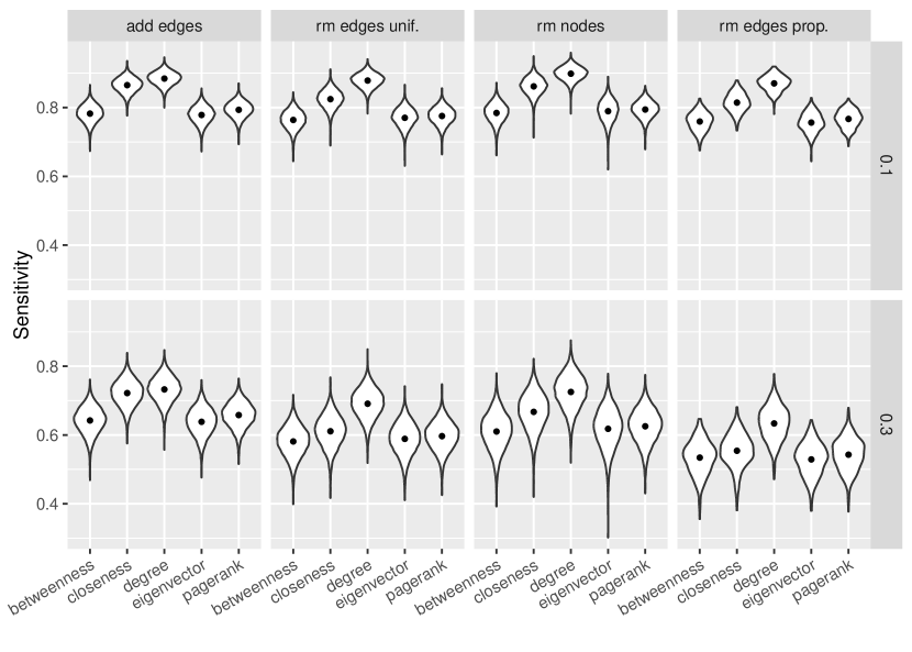
Figure 2: Sensitivity of centrality measures in ER graphs. The violin plots in each panel show the distribution of the sensitivity of the corresponding centrality measure under the influence of different error mechanisms. Mean values are indicated by a black dot.

3 How to estimate the sensitivity of a centrality measure

In a lot of network studies, the observed network data contains sampling errors [25, 32, 35]. But in general, the authors of such studies have no tools to describe the impact of sampling errors on the network measures (e.g., centrality measures) they apply. In general, the assumptions made on sampling errors are mentioned in the limitations, but they are not considered as part of the network model.

The sensitivity concept as introduced in Section 2.2 helps researchers to describe this impact: given the observed network $O$, the (unknown) hidden network $H$, and a centrality measure $c$, $\rho_{c}(O,H)$ measures the probability, that two randomly chosen nodes (with distinct centrality values) have the same order in $c(O)$ and $c(H)$. Hence, $\rho_{c}(O,H)$ is capable to measure the impact of the sampling error on the centrality measure $c$. Thus, the sensitivity can be used to measure the reliability of a centrality measure with respect to sampling errors. We call $\rho_{c}(O,H)$ the “true sensitivity”.

Unfortunately, the hidden network $H$ is not known and thus the true sensitivity cannot be computed explicitly. In this section, we propose two methods for the estimation of the true sensitivity based on the observed network $O$. Moreover, we provide an example for their application and demonstrate how the estimation results can be evaluated.

3.1 Methods to estimate the sensitivity

In this section we propose two methods for the estimation of the true sensitivity $\rho_{c}(O,H)$. In addition to the observed network $O$ and a centrality measure $c$, each of these methods needs an additional assumption.

The first method that we propose is the imputation estimate for the sensitivity of a given centrality measure (“imputation method”). Based on the observed network O and an imputation mechanism $\psi$, we try to “reconstruct” the hidden network from the observed network. Based on the reconstructed network and the observed network, we calculate the estimate for the true sensitivity of the hidden network H and a centrality measure $c$ as follows:

$$\hat{\rho}_{c}^{imp}(O,H):=E(\rho_{c}(O,\psi(O))).$$ (3)

Since $\psi(O)$ is a random graph, $\rho_{c}(O,\psi(O))$ is a random variable and we use the expected value of this expression as the estimate for the sensitivity. The actual form of the imputation mechanism $\psi$ depends strongly on the error mechanism $\varphi$ which has influenced the data collection. However, depending on the network structure and the error mechanism, it might be very difficult to define an appropriate imputation mechanism (see Section 2.1).

The second method that we propose is the iterative estimate for the sensitivity of a given centrality measure (“iterative method”). If we assume that the network of interest has a self-similarity property in the sense that subgraphs of this network have the same sensitivity as the initial network, we can apply the (assumed) error mechanism $\varphi$ to the observed network and calculate the estimate for the true sensitivity of the hidden network H and a centrality measure $c$ as follows:

$$\hat{\rho}_{c}^{iter}(O,H):=E(\rho_{c}(O,\varphi(O))).$$ (4)

Since $\varphi(O)$ is a random graph, $\rho_{c}(O,\varphi(O))$ is a random variable and we use the expected value of this expression as the estimate for the sensitivity. Our experiments indicate that this self-similarity property may exist in many cases even though it is hard to prove that such a property does exist in complex networks.

Both methods do rely on assumptions that are difficult to prove (appropriate imputation mechanism and self-similarity property). However, if these assumptions hold, we should be able to make good estimates for the sensitivity.

3.2 Example for method application

As a fist step to verify whether the proposed methods yield useful results, we apply the four error mechanisms to ER graphs and try to predict the sensitivity using the imputation method as well as the iterative method.

For all combinations of centrality measures and error mechanisms introduced in Section 2 and 2.1, we perform the experiment described below 500 times. For every error mechanism, we consider two cases, a moderate scenario of 10% error level and a more intense scenario with 30% error level. We perform the following steps to simulate erroneous data collection and to collect 3-tuples of true sensitivity, the estimate based on the iterative method, and the estimate based on the imputation method:

1. We generate an ER graph with 100 nodes and edge probability 0.2 and denote it by $H$. This graph represents the (error-free) hidden network.

2. We choose a graph from $\varphi(H)$ and denote it by $O$. This graph represents the observed network which is affected by measurement errors. For evaluation purposes, the true sensitivity $\rho_{c}(H,O)$ is calculated and denoted by $s$.

3. Based on the observed network $O$, two estimates for the true sensitivity are calculated. The imputation estimate ($\hat{\rho}_{c}^{imp}(O,H)$) is denoted by $\hat{s}^{imp}$, the estimate calculated according to the iterative method ($\hat{\rho}_{c}^{iter}(O,H)$) is denoted by $\hat{s}^{iter}$.

The results of these experiments are listed in Table 1. Values in the $s$ columns represent the mean values of the true sensitivity for all 500 runs. The 95th percentile values of the absolute difference between the true sensitivity and the estimate are labeled with $\hat{e}^{imp}$ for the imputation estimates and $\hat{e}^{iter}$ for the iterative estimates. We call this value the absolute error. For example, the average true sensitivity of the betweenness centrality under the influence of the error mechanism add edges random 10% is 0.891 and the imputation estimate of the true sensitivity is in the interval [0.871, 0.911] in 95% of all runs.

Table 1: Results for the estimate of the sensitivity (ER graphs). For all centrality measures, average true sensitivity (column s) and 95th percentile of the absolute error for the estimate ($\hat{e}^{imp}$: imputation method; $\hat{e}^{iter}$: iterative method) are shown. (Values are multiplied by 100 for better readability.)

	betweenness			closeness			degree			eigenvector			PageRank
	s	$\hat{e}^{imp}$	$\hat{e}^{iter}$	s	$\hat{e}^{imp}$	$\hat{e}^{iter}$	s	$\hat{e}^{imp}$	$\hat{e}^{iter}$	s	$\hat{e}^{imp}$	$\hat{e}^{iter}$	s	$\hat{e}^{imp}$	$\hat{e}^{iter}$
error mechanism
add edges (0.1)	89.1	2.0	1.9	93.3	2.4	2.2	94.2	1.8	1.8	89.0	2.0	2.0	89.7	1.9	1.7
rm e prop (0.1)	88.0	2.1	2.1	90.9	2.6	3.2	93.6	1.9	1.8	87.9	2.0	2.0	88.5	1.9	1.9
rm e unif (0.1)	88.2	2.3	2.2	91.2	2.6	2.7	93.9	1.8	2.0	88.5	2.0	2.0	88.8	2.1	1.9
rm nodes (0.1)	89.2	2.8	2.4	93.0	2.2	2.4	94.9	1.8	2.0	89.4	3.0	2.9	89.7	2.0	1.9
add edges (0.3)	82.1	3.0	3.0	86.1	3.7	3.5	86.6	3.4	3.1	81.9	3.5	3.4	82.9	3.0	3.1
rm e prop (0.3)	77.0	5.1	4.8	77.9	5.8	5.9	81.9	5.5	4.4	76.7	5.1	5.0	77.4	5.1	4.6
rm e unif (0.3)	79.2	3.7	3.7	80.6	4.2	3.8	84.6	3.6	4.3	79.5	3.7	3.7	80.0	3.5	3.5
rm nodes (0.3)	80.5	5.0	4.2	83.4	5.3	4.8	86.2	5.0	4.8	80.9	7.0	4.7	81.2	3.9	3.7

It can be seen from Table 1 that there is a wide range of absolute error values (ranging from 0.017 to .07). How should these values be interpreted? For example, the estimates for the sensitivity of the degree centrality and the PageRank under the influence of the add edges 10% error mechanism show approximately the same error values (ranging from 0.017 to 0.019). However, we argue that the estimate for the PageRank works better because the (average) sensitivity of the PageRank is 0.897 while the average sensitivity of the degree centrality is substantially higher (0.942). Therefore, one has to consider the magnitude of the true sensitivity when interpreting the absolute error of an estimate for the sensitivity.

3.3 Evaluating estimation results

The estimate for the true sensitivity is successful if it is “close” to the true sensitivity value. To determine this “closeness”, we calculate the error (absolute difference between true value and estimate) relative to the magnitude of the true sensitivity. On the one hand, if the true sensitivity is low, the estimate does not need to be as accurate as if the true sensitivity is high. On the other hand, we assume that estimating the sensitivity is more difficult if the true sensitivity is relatively low. Moreover, for the evaluation of the “closeness” between the true sensitivity $s$ and an estimate for the true sensitivity $\hat{s}$, we ignore the direction of the deviation. Therefore, we define the weighted error of the estimate as

$$weightederror(s,\hat{s}):=\frac{|s-\hat{s}|}{1-s}\textrm{ for }s<1,$$ (5)

where smaller values indicate better performance. For the ultimate decision whether the estimate is close enough to the target value, we use an indicator function which takes the value one if $weightederror(s,\hat{s})$ is below a given threshold value and zero otherwise.

Figure 3 illustrates the values of this indicator function combined with threshold values of 0.1, 0.3, and 0.5. The dark areas indicate combinations of true sensitivity and estimate of the true sensitivity that we consider successful with respect to the particular threshold value. For example, with a threshold value of 0.1, the estimate of the sensitivity has to be very close to the true value, even for low sensitivity values. In this study, we focus on a threshold value of 0.3. We will use this approach for the remainder of this study to evaluate the performance of the estimate.

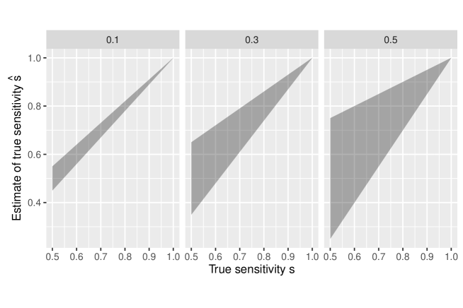
Figure 3: The dark areas in the panels above show successful combinations of true sensitivity $s$ and estimate of the true sensitivity $\hat{s}$ for three threshold values (from left to right: 0.1, 0.3, and 0.5). An estimate of the true sensitivity is only considered successful if the pair $(s,\hat{s})$ is within the dark area.

The weighted error combined with a threshold has two important advantages compared to the absolute error. It takes the variation within the experimental runs into account and requires estimates for higher sensitivity values to be more precise than estimates for lower sensitivity values. Applied to the previous example, we get the following success rates (ratio between the number of successful estimates and the total number of estimates): imputation estimate 0.938, iterative estimate 0.910 in the case of degree and imputation estimate 0.996, iterative estimate 1.000 in the case of PageRank. Using the weighted error, we notice that the estimates for the sensitivity of the degree centrality are very good and estimates for the sensitivity of PageRank are remarkable.

3.4 Results for synthetic graphs

Figure 4 illustrates the performance of the estimates for the experiments on ER graphs. In general, the performance of the estimate for the sensitivity in the context of ER graphs is remarkable. The success rate, i.e. the fraction of cases where the estimate is within the boundaries as defined in Section 3.3, is largely above 90%.

The success rates for all 30% error mechanisms and centrality measures are illustrated in Figure 4. In most cases, there is no difference between iterative and imputation estimate except for cases that involve the closeness centrality. In those cases, the imputation estimate is better if edges or nodes are missing and the iterative method performs better if there are additional edges. This effect diminishes with increasing intensity.

The success rates for betweenness centrality, eigenvector centrality, and PageRank at the same, very high, level, followed by closeness and degree centrality. The latter two show slightly lower (but still high) success rates. The different error mechanisms show similar results. When comparing the 10% and 30% error mechanism, we cannot observe that the success rates are lower for the latter. The converse seems to be the case. The success rates for cases that involve error mechanisms with 30% error level are higher than the corresponding values for 10% error mechanisms. At first, this observation seems counter-intuitive. However, we also observe that the sensitivity decreases with increasing measurement error. Since the sensitivity is lower, the interval for valid estimates becomes larger (Equation 5) and in the case of ER graphs, there is low variation and the success rates become better with increasing intensity.

We also perform the experiment described in Section 3.2 with one difference in the first step: instead of an ER graph, we generate a BA graph [3], 100 nodes, parameter m = 11, undirected). Results for this experiment for cases with 30% error level are shown in Figure 5. In general, the imputation method performs worse than the iterative method. The performance of the imputation method is particularly bad in cases where the betweenness centrality has to be estimated.

In contrast, the iterative method shows high success rates in most of the cases. In cases that involve the degree or closeness centrality, the performance is usually worse that in the remaining cases. There is little difference between the four error mechanisms. The results for the 10% error mechanism (Appendix A) are similar. However, in some cases, we observe lower success rates than in for the corresponding 30% error mechanism.

Figure 4: The success rates for the estimate (ER graphs, 30% error level) are shown in the figure above. The bar length indicates the percentage of successful cases among all trials (success rate). Grey (black) bars represent the success rates for the imputation (iterative) method.

Figure 5: The success rates for the estimate (BA graphs, 30% error level) are shown in the figure above. The bar length indicates the percentage of successful cases among all trials (success rate). Grey (black) bars represent the success rates for the imputation (iterative) method.

4 Application to real-world networks

Here, we apply our methods from Section 3.1 to real-world networks in order to investigate the suitability of these methods for practical application. We use four networks from different domains and thus different structural properties to get an impression how these methods perform on real data. Descriptive statistics for these networks are listed in Table 2.

Table 2: Statistics of real-world networks. If the original network is not connected, we only consider the largest connected component.

Network	Nodes	Edges	Clustering	Density	Diameter	Source
Dolphins	62	159	0.3029	0.0841	8	[26]
Jazz	198	2,742	0.6334	0.1406	6	[14]
Protein	1,458	1,948	0.1403	0.0018	19	[19]
Hamsterster	1,788	12,476	0.1655	0.0078	14	[23]

We use our proposed methods to estimate the sensitivity of five centrality measures under the influence of four error mechanisms. For every error mechanism, we consider two cases, a moderate scenario of 10% error level and a more intense scenario with 30% error level. For every combination of network, centrality measure, and error mechanism, the experimental setup is as follows:

1. Due to the very nature of the hidden networks, we cannot access them. Hence, for the sake of our experiments, we treat the real-world network as the error-free hidden network $H$. (This is a common approach used in existing studies about the sensitivity of centrality measures.)

2. To simulate erroneous data collection, we choose a graph from $\varphi(H)$ and denote it by $O$. This graph represents the observed network which is affected by measurement errors. For evaluation purposes, the true sensitivity $\rho_{c}(H,O)$ is calculated and denoted by $s$.

3. Based on the observed network $O$, two estimates for the true sensitivity are calculated. The imputation estimate ($\hat{\rho}_{c}^{imp}(O,H)$) is denoted by $\hat{s}^{imp}$, the estimate calculated according to the iterative method ($\hat{\rho}_{c}^{iter}(O,H)$) is denoted by $\hat{s}^{iter}$.

For every combination, we perform this experiment 500 times. To evaluate the results, we use the procedures described in Section 3.3.

4.1 Results for real-world networks

In this section, we study how our methods for estimating the sensitivity of centrality measures perform on real-world networks. Regarding the iterative estimates, we observe a fair amount of cases with high success rate. However, the results for empirical networks are more heterogeneous than the results for Erdős–Rényi and Barabási–Albert networks (Section 3.4). But since the real-world networks are more complex than graphs generated by these procedures, we expected that our estimation methods would not work as well for real-world networks compared to synthetic networks.

The results for the estimate of the sensitivity of centrality measures in real-world networks are shown in Figure 6 and 7. First, we focus on the results for error mechanisms with 10% error level (Figure 6). Comparing both estimation methods, it turns out that the iterative method is at least as good as the imputation method, except for a few cases where the former is slightly better. Hence, we first focus on the estimates of the iterative method. The iterative estimate for PageRank works in virtually all cases, regardless of the specific network or error mechanism. Among the four networks, the success rates for the Dolphins network are usually the lowest. It is reasonable to assume that this effect is due to the small size of the Dolphin network (62 nodes, 159 edges). If we focus our discussion on the three larger networks, we observe high success rates for the estimates of the sensitivity of closeness, betweenness, and eigenvector centrality if edges are missing uniformly or proportional. For these networks, the estimates for the sensitivity of the eigenvector centrality also work if the measurement errors lead to too many edges in the observed network. The results suggest, that the error mechanism missing nodes is most difficult for the estimate. There is no strong relationship between sensitivity and the success rate, higher sensitivity values are not easier to estimate. The average sensitivity values for all real-world networks can be found in Appendix A.

Comparing Figure 6 and 7 shows that the success rates for the iterative method become lower with an increasing level of error. It is more difficult to estimate the sensitivity for higher levels of measurement errors. The estimate for the sensitivity of PageRank still works for error mechanisms additional edges and missing edges. If we focus on the three largest networks, the cases involving betweenness and closeness centrality show good success rates if edges are missing (uniformly and proportional). Cases involving the eigenvector centrality show good success rates if edges are missing uniformly and for the error mechanism additional edges.

We observe cases with a subpar performance for 10% error level where the success rates continue to decrease. For example, the Jazz network with additional edges in combination with the closeness and betweenness centrality. There are few cases that show good performance for 10% error level but work barely for 30% error level (e.g., if edges are missing proportionally in the Jazz network and we try to estimate the sensitivity of eigenvector centrality or PageRank).

The results for the imputation estimates of the sensitivity are rather different. There is no centrality measure or error mechanism where this method shows high success rates for all four networks. In some cases, the imputation estimate for error levels of 30% is better than the imputation estimate for the corresponding 10% case (e.g., PageRank and additional edges). Most of these situations occur when the error mechanism is additional edges.

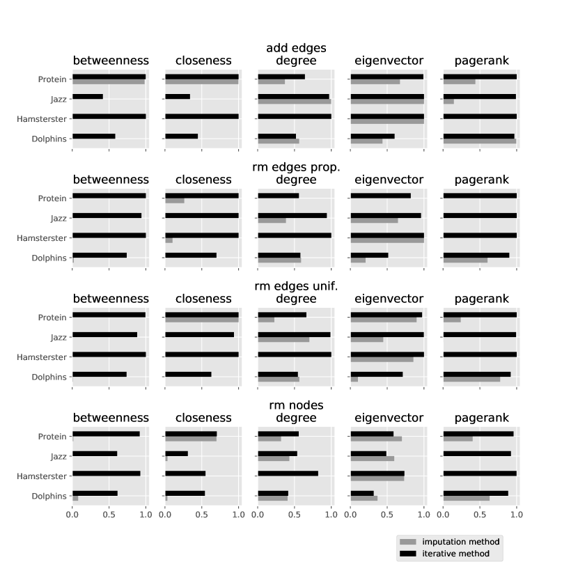
Figure 6: The success rates for the estimate (real-world networks, 10% error level) are shown in the figure above. The bar length indicates the percentage of successful cases among all trials (success rate). Grey (black) bars represent the success rates for the imputation (iterative) method.

Figure 7: The success rates for the estimate (real-world networks, 30% error level) are shown in the figure above. The bar length indicates the percentage of successful cases among all trials (success rate). Grey (black) bars represent the success rates for the imputation (iterative) method.

5 Discussion and conclusion

Errors in network data are a ubiquitous problem in network analysis and previous studies have shown that these errors can have a severe impact on the reliability of centrality measures. Most studies that use centrality measures, however, rarely discuss the ramifications that measurement errors have on their analyses. Usually, these studies mention that the observed data might contain errors, but analyses are performed as if the data is error-free. Even though the reliability of centrality measures has been studied extensively, there is no technique that allows researchers to assess the reliability of centrality measures in the case of imperfect observed data.

In the first part of this study, we introduced concepts to describe such a technique. We defined an easy-to-interpret metric, the sensitivity, to measure the reliability of centrality measures. Additionally, we presented the concept of error mechanisms, which model measurement errors as random graphs. We applied these concepts to ER graphs and the results are consistent with previous research [6].

In the main part of this study, we proposed two methods (“imputation method” and “iterative method”) that allow the researcher to estimate the sensitivity of the error-free (hidden) network, given the observed network and some assumptions about the measurement error.

Our experiments showed that both methods performed very well on ER graphs. In the case of BA graphs and real-world networks, the imputation method rarely worked and should therefore not be used. These findings extend those of Huisman (2009) [18], confirming that imputation methods are only useful in a few specific situations. Surprisingly, the method that is easier to calculate yielded better results. We could identify cases where the iterative method showed remarkable performance. It worked especially well for the PageRank for all error mechanisms with 10% error level. If the error level increased to 30%, the iterative method still showed good performance if edges were missing uniformly at random or if there were spurious edges. If 10% of the edges were missing uniformly at random or proportional and the network was not too small, the iterative method performed well for all centrality measures except for the degree centrality. The sensitivity values for the degree centrality were, however, relatively high.

Our results provide compelling evidence that the iterative method is, in principle, a suitable technique for the estimation of the sensitivity of centrality measures. Hence, it is a promising first step that helps researchers to assess the impact of measurement errors on their observed network data. Although the iterative method works in well in many cases, there are limitations. There is a need to clarify the conditions under which the self-similarity assumption does not hold true and thus identify, based on the observed network, the cases where the iterative method should not be used. Another important question for future studies is to determine more suitable imputation mechanisms and thus improving the performance of the imputation method.

Appendix A Additional results

Figure 8: The success rates for the estimate (ER graphs, 10% error level) are shown in the figure above. The bar length indicates the percentage of successful cases among all trials (success rate). Grey (black) bars represent the success rates for the imputation (iterative) method.

Figure 9: The success rates for the estimate (BA graphs, 10% error level) are shown in the figure above. The bar length indicates the percentage of successful cases among all trials (success rate). Grey (black) bars represent the success rates for the imputation (iterative) method.

Table 3: The average sensitivity values for the real-world networks are listed in the table below. (Values are multiplied by 100 for better readability.)

Centrality measure		bc		cc		dc		ec		pr
Level of error		0.1	0.3	0.1	0.3	0.1	0.3	0.1	0.3	0.1	0.3
Error mechanism	Network
Add edges	Dolphins	80.8	76.2	82.1	76.3	98.5	94.2	89.3	81.5	93.0	87.6
	Hamsterster	84.5	81.3	94.4	90.5	97.7	94.1	96.4	93.3	91.7	87.7
	Jazz	82.3	79.5	90.4	86.5	98.2	95.9	97.0	94.1	95.0	92.4
	Protein	92.3	86.1	90.8	83.0	99.0	95.1	91.1	83.7	89.6	81.6
Remove edges (prop.)	Dolphins	91.9	83.3	93.1	85.0	98.5	92.2	92.6	76.6	93.7	85.7
	Hamsterster	97.1	93.4	95.7	89.5	99.5	97.6	96.3	90.7	97.6	94.6
	Jazz	96.0	91.7	95.5	90.7	98.5	95.3	97.2	94.1	97.0	93.3
	Protein	95.4	89.7	85.0	67.2	99.6	96.9	80.2	63.0	93.5	85.6
Remove edges (unif.)	Dolphins	91.4	82.9	93.2	85.3	98.4	93.3	93.7	85.5	93.4	86.1
	Hamsterster	96.0	91.2	96.6	91.6	99.3	97.0	96.8	92.6	96.3	92.1
	Jazz	95.1	89.6	96.2	91.5	98.4	95.8	97.5	94.9	96.5	93.1
	Protein	95.5	90.7	88.8	75.8	99.3	95.5	87.9	76.3	92.2	82.9
Remove nodes	Dolphins	90.9	82.8	92.2	84.5	98.4	93.8	90.1	80.7	93.5	87.1
	Hamsterster	96.4	91.7	96.7	91.9	99.3	97.0	96.7	92.4	96.5	92.4
	Jazz	95.5	90.5	96.8	92.8	98.7	96.4	97.0	93.5	97.3	94.4
	Protein	95.6	91.2	88.3	75.0	99.4	95.4	87.0	75.3	92.2	83.1

References

- [1] P. D. Allison. Missing data: Quantitative applications in the social sciences. British Journal of Mathematical and Statistical Psychology, 55(1):193–196, 2002.
- [2] A.-L. Barabási. Network Science. Cambridge University Press, 2016.
- [3] A.-L. Barabási and R. Albert. Emergence of Scaling in Random Networks. Science, 286(October):509–512, 1999.
- [4] B. Bollobás and O. Riordan. Mathematical results on scale-free random graphs. Handbook of Graphs and Networks: From the Genome to the Internet, pages 1–38, 2002.
- [5] P. Bonacich. Power and Centrality: A Family of Measures. American Journal of Sociology, 92(5):1170–1182, 1987.
- [6] S. P. Borgatti, K. M. Carley, and D. Krackhardt. On the robustness of centrality measures under conditions of imperfect data. Social Networks, 28(2):124–136, 2006.
- [7] S. Brin and L. Page. The Anatomy of a Large-scale Hypertextual Web Search Engine. In Proceedings of the Seventh International World-Wide Web Conference (WWW 1998), pages 107–117, 1998.
- [8] C. T. Butts. Network inference, error, and informant (in)accuracy: A Bayesian approach, 2003.
- [9] E. Costenbader and T. W. Valente. The stability of centrality measures when networks are sampled. Social Networks, 25(4):283–307, 2003.
- [10] G. Csardi and T. Nepusz. The igraph Software Package for Complex Network Research. InterJournal, Complex Systems, (1695):1–9, 2006.
- [11] T. L. Frantz and K. M. Carley. Reporting a network’s most-central actor with a confidence level. Computational and Mathematical Organization Theory, pages 1–12, 2016.
- [12] T. L. Frantz, M. Cataldo, and K. M. Carley. Robustness of centrality measures under uncertainty: Examining the role of network topology. Computational and Mathematical Organization Theory, 15(4):303–328, 2009.
- [13] L. C. Freeman. Centrality in social networks conceptual clarification. Social Networks, 1(3):215–239, 1978.
- [14] P. M. Gleiser and L. Danon. Community structure in jazz. Advances in Complex Systems, 6(4):565–573, 2003.
- [15] L. A. Goodman and W. H. Kruskal. Measures of association for cross classifications. Journal of the American Statistical Association, 49(268):732–764, 1954.
- [16] M. S. Handcock and K. J. Gile. Modeling social networks from sampled data. The Annals of Applied Statistics, 4(1):5–25, 2010.
- [17] S. Havlin and R. Cohen. Complex networks: structure, robustness and function. 2010.
- [18] M. Huisman. Imputation of missing network data: some simple procedures. Journal of Social Structure, 10(1):1–29, 2009.
- [19] H. Jeong, S. P. Mason, A.-L. Barabasi, and Z. N. Oltvai. Lethality and centrality in protein networks. Nature, 411(6833):41–42, may 2001.
- [20] M. Kim and J. Leskovec. The Network Completion Problem: Inferring Missing Nodes and Edges in Networks. SIAM International Conference on Data Mining, pages 47–58, 2011.
- [21] P. J. Kim and H. Jeong. Reliability of rank order in sampled networks. European Physical Journal B, 55(1):109–114, 2007.
- [22] D. Koschützki, K. Lehmann, and L. Peeters. Centrality Indices. In U. Brandes and T. Erlebach, editors, Network Analysis: Methodological Foundations, pages 16–61. Springer Berlin Heidelberg, 2005.
- [23] J. Kunegis. KONECT - The koblenz network collection. In WWW 2013 Companion - Proceedings of the 22nd International Conference on World Wide Web, 2013.
- [24] J.-s. Lee and J. Pfeffer. Robustness of Network Centrality Metrics in the Context of Digital Communication Data. Proceedings of the 48th Hawaii International Conference on System Sciences, 2015.
- [25] M. Leecaster, D. J. A. Toth, W. B. P. Pettey, J. J. Rainey, H. Gao, A. Uzicanin, and M. Samore. Estimates of social contact in a middle school based on self-report and wireless sensor data. PLoS ONE, 11(4), 2016.
- [26] D. Lusseau, K. Schneider, O. J. Boisseau, P. Haase, E. Slooten, and S. M. Dawson. The bottlenose dolphin community of doubtful sound features a large proportion of long-lasting associations: Can geographic isolation explain this unique trait? Behavioral Ecology and Sociobiology, 54(4):396–405, 2003.
- [27] M. E. J. Newman. Measurement errors in network data. eprint arXiv:1703.07376, mar 2017.
- [28] Q. Niu, A. Zeng, Y. Fan, and Z. Di. Robustness of centrality measures against network manipulation. Physica A: Statistical Mechanics and its Applications, 438:124–131, 2015.
- [29] J. Platig, E. Ott, and M. Girvan. Robustness of network measures to link errors. Physical Review E - Statistical, Nonlinear, and Soft Matter Physics, 88(6), 2013.
- [30] D. B. Rubin. Multiple Imputation after 18+ Years. Journal of the American Statistical Association, 91(434):473–489, 1996.
- [31] J. L. Schafer and J. W. Graham. Missing data: Our view of the state of the art. Psychological Methods, 7(2):147–177, 2002.
- [32] J. Schulz. Using Monte Carlo simulations to assess the impact of author name disambiguation quality on different bibliometric analyses. Scientometrics, 107(3):1283–1298, 2016.
- [33] J. A. Smith and J. Moody. Structural Effects of Network Sampling Coverage I: Nodes Missing at Random. Social networks, 35(4), oct 2013.
- [34] J. A. Smith, J. Moody, and J. H. Morgan. Network sampling coverage II: The effect of non-random missing data on network measurement. Social Networks, 48:78–99, 2017.
- [35] C. Wang, C. T. Butts, J. R. Hipp, R. Jose, and C. M. Lakon. Multiple imputation for missing edge data: A predictive evaluation method with application to Add Health. Social Networks, 45:89–98, 2016.
- [36] D. J. Wang, X. Shi, D. A. McFarland, and J. Leskovec. Measurement error in network data: A re-classification. Social Networks, 34(4):396–409, 2012.