A Comparison of Maps and Power Spectra Determined from South Pole Telescope and Planck Data

Abstract

We study the consistency of 150 GHz data from the South Pole Telescope (SPT) and 143 GHz data from the Planck satellite over the patch of sky covered by the SPT-SZ survey. We first visually compare the maps and find that the residuals appear consistent with noise after accounting for differences in angular resolution and filtering. We then calculate (1) the cross-spectrum between two independent halves of SPT data, (2) the cross-spectrum between two independent halves of Planck data, and (3) the cross-spectrum between SPT and Planck data. We find the three cross-spectra are well-fit (PTE = 0.30) by the null hypothesis in which both experiments have measured the same sky map up to a single free calibration parameter—i.e., we find no evidence for systematic errors in either data set. As a by-product, we improve the precision of the SPT calibration by nearly an order of magnitude, from 2.6% to 0.3% in power. Finally, we compare all three cross-spectra to the full-sky Planck power spectrum and find marginal evidence for differences between the power spectra from the SPT-SZ footprint and the full sky. We model these differences as a power law in spherical harmonic multipole number. The best-fit value of this tilt is consistent among the three cross-spectra in the SPT-SZ footprint, implying that the source of this tilt is a sample variance fluctuation in the SPT-SZ region relative to the full sky. The consistency of cosmological parameters derived from these datasets is discussed in a companion paper.

1. Introduction

One of the most remarkable results of modern cosmology is that a simple six-parameter model, usually referred to as the Lambda Cold Dark Matter ($\Lambda\mathrm{CDM}$) model, can fit the full range of cosmological observations. With the precision of cosmological observables now reaching the level of a few percent, however, several small discrepancies in the inferred parameter values are attracting attention.

These discrepancies show up in three places. The first is in the inferred parameter values from the CMB compared to some observations of the local universe. For example, the amplitude of local density fluctuations, $\sigma_{8}$, that is measured from observations of large scale structure appears lower than the $\sigma_{8}$ value implied by cosmic microwave background (CMB) measurements (Planck Collaboration et al., 2016f). There is also some tension between direct measurements of the Hubble parameter $H_{0}$ and the value derived from CMB measurements (Planck Collaboration et al., 2014c, 2016e; Riess et al., 2011, 2016).

Second, there are mild (1-2$\sigma$) discrepancies between parameter values derived from observations of the CMB by different experiments. In particular, the best-fit parameters of the $\Lambda\mathrm{CDM}$ model given Planck satellite measurements of CMB temperature and polarization power spectra (Planck Collaboration et al., 2016c) are somewhat different from those derived from earlier CMB data, whether from the Wilkinson Microwave Anisotropy Probe (WMAP) satellite (Hinshaw et al., 2013), from the combination of WMAP data and data from the South Pole Telescope (SPT, Hou et al. 2014), or from WMAP + SPT plus data from the Atacama Cosmology Telescope (ACT, Calabrese et al. 2013).

Finally, work has been done on the internal consistency of $\Lambda$CDM model parameter values from different subsets of the Planck data. Addison et al. (2016) recently pointed out that the matter density inferred from Planck data at $\ell<1000$ is 2.5 $\sigma$ discrepant from that inferred from Planck data at $\ell>1000$. In response, Planck Collaboration et al. (2017) show that after correcting for certain approximations in the Addison et al. (2016) analysis, and taking into account the fact that matter density had been singled out as the most discrepant parameter, the global discrepancy is only 1.6 $\sigma$.

Taken together, these low-level discrepancies have led some to speculate that we are seeing evidence of a potential failure of the $\Lambda\mathrm{CDM}$ model (Wyman et al., 2014; Battye & Moss, 2014), systematic errors in the analysis of the low-redshift probes (Efstathiou et al., 2014), or systematic errors in the Planck data (Planck Collaboration et al., 2017). The analysis presented in this paper is motivated by the fact that it is the high-$\ell$ temperature data from Planck that are driving the parameter shifts of interest (Addison et al., 2016; Planck Collaboration et al., 2017). In terms of the measurement uncertainties, data from the 2540-square-degree SPT-SZ survey yield constraints within a factor of 2 of the Planck constraints at $\ell\gtrsim 1700$ and better than Planck at $\ell\gtrsim 2100$ (Story et al., 2013, hereafter S13). The SPT-SZ data are thus a logical choice for consistency checks of the high-$\ell$ Planck data.

In this work, we present the first comparison between Planck and SPT data over the same patch of sky. Checks have previously been performed at the power-spectrum and cosmological-parameter level, for instance in Planck Collaboration et al. (2014c) and Planck Collaboration et al. (2016e), and the two data sets have been shown to be roughly consistent, but again with some low-level discrepancies. The strength of power-spectrum and parameter comparisons using the full datasets are limited by the sample variance of the SPT data at lower $\ell$ and Planck noise at higher $\ell$. By limiting the comparison to CMB modes measured by both experiments, we can greatly reduce the sample variance to sharpen the consistency tests between the two data sets.

Here we compare the SPT-SZ data in the 150 GHz band and Planck full-mission data in the 143 GHz band, restricted to the SPT-SZ observing region. We calculate angular cross-spectra of the SPT and Planck maps ($150\times 143$), and, for comparison, the cross-spectrum of one half of SPT data with the other half ($150\times 150$), and the cross-spectrum of one half of Planck data with the other half ($143\times 143$). We calculate the difference between the SPT $150\times 150$ spectrum and the other two, as well as the ratio of the SPT $150\times 150$ spectrum to the others. Using simulated observations of mock skies (including realistic noise for both experiments), we calculate the expected uncertainty in these differences and ratios, and we use this to calculate the $\chi^{2}$ and probability to exceed this $\chi^{2}$ under the null hypothesis that there are no systematic biases between the experiments. This investigation is similar to that performed by Louis et al. (2014) on ACT and Planck data over 592 deg² of sky and two observing bands (143/148 GHz and 217/218 GHz), the conclusion of which was that ACT and Planck measured statistically consistent CMB fluctuations over that patch of sky.

This paper is organized as follows. In Section 2, we discuss the SPT 150 GHz and Planck 143 GHz temperature maps in the 2540 $\text{deg}^{2}$ patch of sky that constitutes the whole of the SPT-SZ survey region. In Section 3 we present how power spectra are calculated from the maps and the simulations generated to de-bias the data and build the covariance matrix. In Section 4 we compare the power spectra and use simulations to test the null hypothesis that the two experiments are measuring the same sky, and we discuss these results in the context of comparisons between SPT and full-sky Planck data. We present our conclusions in Section 5.

2. Data

The main goal of this work is to compare maps and power spectra from the SPT 150 GHz and Planck 143 GHz data sets within the $2540\deg^{2}$ SPT-SZ survey area. As an overview of the two datasets, Figure 1 shows a sky map of Planck HFI 143 GHz full-mission data, with the SPT-SZ survey area outlined by a solid black curve. In this section, we discuss details of the map-making and instrumental characteristics of each experiment.

2.1. SPT

The SPT is a 10-meter telescope located at the Amundsen-Scott South Pole station. From 2008 to 2011, the first camera on the SPT, a three-band bolometer array known as the SPT-SZ camera, was used to conduct a survey of $\sim$2500 deg² of the Southern sky with low Galactic dust contamination, referred to as the SPT-SZ survey. As shown in Figure 1, the survey area is a contiguous region extending from $20^{\mathrm{h}}$ to $7^{\mathrm{h}}$ in right ascension (R.A.) and from $-65^{\circ}$ to $-40^{\circ}$ in declination. The survey was conducted by observing a series of 19 areas, ranging in area from roughly 100 to 300 square degrees, which together form the full survey region (see, e.g., S13, Figure 2). If not specified, in this paper we use “field” to refer to individual observing areas of SPT-SZ.

There were approximately 200 observations of each field, with each individual observation taking roughly 2 hours. Estimates of the primary CMB temperature power spectrum from this survey, and the resulting cosmological interpretation, are discussed in Keisler et al. (2011, hereafter K11), S13, and Hou et al. (2014). Our analysis is identical to that of S13 up to the single-observation map step. We briefly review that part of the analysis here and refer the reader to K11 and S13 for more details.

To process time-ordered data (TOD) into maps, the TOD from each SPT detector are first filtered and multiplied by a calibration factor. The filtering steps important for this analysis are a high-pass filter and the subtraction of a common mode across all detectors in each of the six 160-element module in the focal plane. The high-pass filter cuts off signals below a temporal frequency corresponding to an angular frequency along the scan direction of $\ell=270$. The common-mode subtraction acts as an isotropic high-pass filter with a cutoff at roughly $\ell=500$. In both of these filtering steps, bright point sources ($S>50$ mJy at 150 GHz) are masked to avoid large filtering artifacts.

The TOD from individual SPT detectors are then binned into maps using inverse-variance weighting, i.e., TOD samples corresponding to times when an individual detector was pointed at a particular pixel are averaged together using using inverse-variance weighting, then assigned to that pixel. Maps are made using the oblique Lambert equal-area azimuthal projection (Snyder, 1987) with 1-arcmin square pixels.

The SPT maps are simply binned-and-averaged maps of filtered data and thus are biased representations of the sky. The signal in these maps is the true sky signal convolved with the instrument beam, the effect of the TOD filtering, and the effect of binning. Beams are discussed below, and the filter transfer function is estimated through simulations, as discussed in Section 3.3.

We use the S13 estimates of the SPT 150 GHz beam transfer function $B_{\ell}$ and its uncertainty, and refer the reader to S13 for more details. Briefly, the main lobe is measured using bright point sources in the survey fields, while the sidelobes are measured using observations of Jupiter. Venus observations are used to stitch the two together. The main lobe of the beam is well-approximated by a 1.2-arcmin FWHM Gaussian. The beam uncertainty arises from several statistical and systematic effects, including residual atmospheric noise in the maps of Venus and Jupiter, and the weak dependence of $B_{\ell}$ on the choice of radius used to stitch the inner and outer beam maps.

The TOD from each detector in each observation is calibrated using the response to an internal thermal source, which is in turn tied to the brightness of the Galactic H $\scriptstyle{\rm II}$ region RCW38. For details of this calibration, see Schaffer et al. (2011). The full-depth maps are then compared to CMB satellite data to provide the overall absolute calibration. In K11 and S13, the power spectrum of the full-depth maps was compared to the full-sky WMAP estimate of the CMB power spectrum in the multipole range $650\leq\ell\leq 1000$. For this work, we initially use the calibration determined in George et al. (2015), using the comparison of SPT power spectra to the full-sky Planck power spectrum in the multipole range $670\leq\ell\leq 1170$; however, the map-based comparison to Planck undertaken here ends up providing a significantly more precise absolute calibration, as detailed in Section 4.2.

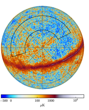
Figure 1.— The celestial southern hemisphere of CMB data from Planck HFI 143 GHz data. The black curve outlines the SPT-SZ survey coverage. The image is oriented such that the line of $0^{\mathrm{h}}$ right ascension extends from the center to the top of the hemisphere, and right ascension increases counter-clockwise.

2.2. Planck

The Planck satellite (Planck Collaboration et al., 2014a) was launched in 2009 by the European Space Agency, with the goal of measuring the CMB temperature and polarization anisotropy with significantly better sensitivity, angular resolution, and wavelength coverage than was achieved by its space predecessor, the WMAP mission (Bennett et al., 2013). Planck mapped the full sky in nine bands, ranging in frequency from 30 to 857 GHz. In this work, we use HFI data from the 2015 data release. Specifically, we use the 143 GHz full-mission, halfmission-1, and halfmission-2 maps downloaded from the NASA/IPAC Infrared Science Archive (IRSA).

In this work, we use a cross-spectrum pipeline similar to that used in K11 and S13 to compare SPT and Planck data on the SPT-SZ sky patch. To use this pipeline for Planck data, the Planck maps must have the same pixelization, projection, and field definitions as the SPT maps. To achieve this, we create mock TOD using the Planck 143 GHz full-mission or half-mission maps and the SPT pointing and detector weight information from individual SPT observations. The mock TOD are then binned into maps in the same manner as the real SPT TOD, using the same projection and pixelization. Instead of using the SPT bandpass filtering, a much simpler high-pass filter is applied to the Planck mock TOD to simply remove the signals on scales with $\ell<100$. Our simulations show that applying this simple high-pass filter greatly improves the numerical stability of our unbiased power spectrum calculations. In the power spectrum analysis described below, we use the projected Planck maps generated from the map-making pipeline with this simple high-pass filter applied to the Planck mock TOD.

The Planck 143 GHz beam has been measured using the Planck TOD around planets, such as Mars, Jupiter and Saturn (Planck Collaboration et al., 2014b, 2016a). The beam window function $B(\ell)$ for individual frequency detector sets has been released by the Planck collaboration as part of the “Reduced Instrument Model” (RIMO). From the 2013 Planck data realease to the 2015 data release, there was a marked improvement in the beam characterization, such that the uncertainty on the 2015 beam window functions for 143 GHz data is at the 0.1% level for the $\ell$ range of interest to this work.

3. Power Spectrum

We now turn to the methodology for calculating unbiased cross-spectra of SPT 150 GHz maps and Planck 143 GHz maps. We introduce the power spectrum estimator in Section 3.1. Simulations are used in several places while estimating the power spectra; we describe how these simulations are generated in Section 3.2. We discuss how these simulations are used to estimate the SPT filter transfer function in Section 3.3 and to calculate the noise and sample-variance parts of the power spectrum covariance in Section 3.4.1. We describe how beam uncertainty is incorporated into the analysis in Section 3.4.2. Finally, we discuss how to calculate the window functions needed to compare the binned cross-spectrum estimates—or “bandpowers”—to a theory spectrum in Section 3.4.3.

3.1. Power Spectrum Estimator

We use an estimator similar to that used in K11 and S13 to calculate the various cross-spectra in this work. Each cross-spectrum is calculated by correlating maps made from different observations of the same field—either correlating full-depth SPT maps with full-depth Planck maps or correlating two half-depth maps from the same experiment. In the latter case, there is a noise penalty relative to K11 or S13 who used $\mathcal{O}(100)$ independent maps depending on the field. However, the noise penalty is largely insignificant for the SPT maps (less than 2% in power) on the angular scales of interest, and it is unavoidable for the Planck maps because a larger number of independent splits are not publicly available. We mask and zero-pad each map before calculating its 2-dimensional Fourier transform, $\tilde{m}_{\boldsymbol{\ell}}$. The mask is a product of an apodization window and a point-source mask. The maps and masks are zero-padded before Fourier-transforming such that each Fourier-space pixel has a width of $\delta_{\ell}=5$. The raw bandpowers are the binned average of the cross-spectra between two maps $A$ and $B$ within a multipole bin $b$:

$$\hat{D}_{b}^{A\times B}=\langle\frac{\ell(\ell+1)}{2\pi}H_{\boldsymbol{\ell}}\mathrm{Re}\left[\tilde{m}^{A}_{\boldsymbol{\ell}}\tilde{m}^{B*}_{\boldsymbol{\ell}}\right]\rangle_{\ell\in b}.$$ (1)

For the SPT-only power spectrum, $A$ and $B$ are the two SPT half-survey maps; for the SPT and Planck cross-spectrum, $A$ and $B$ are the full mission maps of each experiments; and for the Planck-only 143 power spectrum, $A$ and $B$ are the two Planck half-mission maps. $H_{\boldsymbol{\ell}}$ in the above equation represents the 2-dimensional weighting of the Fourier modes that was used by S13 to handle the anisotropic noise in the SPT maps. While this weighting is suboptimal for Planck data, we still use the same S13-derived weighting for all bandpowers to minimize the differential sample variance between cross-spectra.

Since the input maps are biased estimates of the true sky, due to effects as the application of a mask to the maps, the raw bandpowers $\hat{D}_{b}$ are a biased estimate of the true bandpowers, $D_{b}$. The biased and unbiased estimates are related by

$$\hat{D}_{b^{\prime}}\equiv K_{b^{\prime}b}D_{b}\,,$$ (2)

where

$$K_{bb^{\prime}}=P_{b\ell}\left(M_{\ell\ell^{\prime}}\,F_{\ell^{\prime}}B^{2}_{\ell^{\prime}}\right)Q_{\ell^{\prime}b^{\prime}},$$ (3)

$Q_{\ell^{\prime}b^{\prime}}$ is the binning operator and $P_{b\ell}$ is its reciprocal, $M_{\ell\ell^{\prime}}$ is the mode-coupling matrix, $F_{\ell}$ is the filter transfer function which accounts for the signal suppressed by TOD filtering, and $B_{\ell}$ is the beam function. For details on the unbiasing procedure, see K11, S13, and Hivon et al. (2002).

The unbiased bandpowers are calculated on a field-by-field basis and then combined. We combine the bandpowers obtained from individual fields using the effective area of single fields as the weighting, as in K11 and S13.

3.2. Simulations

We use simulations both in the calculation of the bandpowers and to characterize the degree of consistency between the SPT and Planck cross-spectra over the SPT-SZ survey region. In this section, we turn our attention to how these simulations are created and used. The final product of this procedure is 400 sets of simulated unbiased bandpowers for each of the three combinations of data ($150\times 150$, $150\times 143$, and $143\times 143$).

3.2.1 Sky Signals

Our simulations include the following components: 1) a gravitationally lensed CMB signal, 2) thermal and kinematic Sunyaev-Zel’dovich (SZ) signals, 3) the cosmic infrared background (CIB) signal, and 4) emission from radio galaxies. We generate 400 realizations of the lensed CMB with LensPix (Lewis, 2005), based on the best-fit $\Lambda\mathrm{CDM}$ model from Planck 2015 $\mathrm{TT,TE,EE+lowP+lensing}$ (Planck Collaboration et al., 2016e). Modes are generated out to $\ell_{\mathrm{max}}=8000$, well above the angular multipoles, $\ell<2500$, used in this comparison. The maps are stored in HEALPix (Górski et al., 2005) format with resolution parameter $N_{\mathrm{side}}=8192$.

Unlike S13 which used Gaussian realizations for all extragalactic foregrounds, here we generate realizations of individual sources for the bright CIB galaxies ($6.4\,\mathrm{mJy}<S<50\,\mathrm{mJy}$) and all radio galaxies (up to the flux cut at 50 mJy). The bright CIB galaxies are drawn from the modeled $\mathrm{d}N/\mathrm{d}S$ of Cai et al. (2013), while the radio galaxy $\mathrm{d}N/\mathrm{d}S$ is taken from De Zotti et al. (2005). In both cases, the amplitudes of the $\mathrm{d}N/\mathrm{d}S$ distribution are calibrated by the actual observations of Mocanu et al. (2013) at 150 GHz.

The other extragalactic foregrounds, the thermal and kinematic SZ signals and the low-flux CIB, are treated as Gaussian. The shapes of the thermal and kinematic SZ angular power spectra are taken from the Shaw et al. (2010) and Shaw et al. (2012) models respectively, with the amplitudes set to the median values from George et al. (2015), $D_{3000}^{\rm tSZ}=4.38\,\mathrm{\mu K}^{2}$ and $D_{3000}^{\rm kSZ}=1.57\,\mathrm{\mu K}^{2}$. We similarly draw upon the median values and templates from George et al. (2015) for the CIB terms. The clustered CIB spectrum is taken to follow $D_{\ell}\propto\ell^{0.8}$ with an amplitude $D_{3000}^{c}=3.46\,\mathrm{\mu K}^{2}$. The shot-noise or “Poisson” CIB power from galaxies dimmer than $6.4\,\mathrm{mJy}$ is taken to be $D_{3000}^{\rm P}=9.16\,\mathrm{\mu K}^{2}$.

Each component is scaled appropriately to the effective frequency of the SPT or Planck maps and then coadded together to create the final sky realization.

3.2.2 Planck Noise Simulations

The Planck collaboration released the 8th Full Focal Plane (FFP8) simulation in the 2015 data release (Planck Collaboration et al., 2016d). There are 1000 full-mission FFP8 noise simulations available at NERSC. We use the FFP8 full-mission simulations to create noisy Planck-like realizations to characterize the noise contribution to the SPT-Planck cross ($150\times 143$) bandpowers as discussed in Section 4.2.

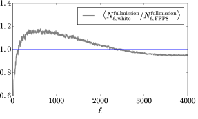
Figure 2.— Averaged ratio of the noise power spectrum between the white-noise realizations and Planck FFP8 noise simulations within the SPT survey area. While we use the full FFP8 noise simulations for the most-constraining set of bandpowers (SPT $\times$ Planck), we use the simpler white-noise realizations when estimating uncertainties for the cross-spectrum between half-survey Planck maps.

The FFP8 noise simulations are only available for the full-mission data, and thus cannot be used for the Planck half-mission cross-spectrum. To create unbiased Planck 143 GHz bandpowers within the SPT area, we also generate half-mission noise simulations to characterize the noise contribution to the Planck-Planck ($143\times 143$) bandpowers as presented in Section 4.2. The half-mission noise simulations are based on the pixel-space noise variance released by the Planck collaboration along with the half-mission observation maps. We approximate the Planck map noise as Gaussian and uncorrelated between pixels (“white”) for the half-mission noise simulations.

To test this white-noise approximation, we compare the noise power spectrum over the SPT survey area from 100 of these Gaussian white-noise realizations to 100 FFP8 full-mission noise simulations. The average power ratio is plotted in Figure 2. Clearly, the white-noise realizations overestimate the noise power for $150<\ell<2200$, i.e. most angular multipoles of interest. This implies that the Planck noise contribution is overestimated in our Planck-only bandpowers, at a maximum level of roughly 15% and a mean level of $\lesssim 10\%$ across the $\ell$ range of interest. We discuss the possible impact of this overestimate on our results in Section 4.2 and find that our main conclusions would likely be unchanged had we used more realistic noise simulations for the Planck-only bandpowers.

3.2.3 SPT Noise Realizations

SPT noise realizations are created directly from the data. For each individual SPT observation of each SPT-SZ survey field, we create a residual map which is the difference between a map made from all left-going telescope scans and a map made from all right-going telescope scans. There are approximately 200 jackknife maps for each field (the number of individual $\sim$2-hour observations). We use these maps to create the noise part of the simulated SPT observations. For each field, we multiply +1 or -1 randomly to the residual maps and coadd them together to form one noise realization. Using this method, we create 400 noise realizations.

With the same method, we also create SPT noise realizations of the first and second half sets of observations by coadding the residual maps of half of the observations within one field. Similar to the half-mission noise simulations for Planck  we use the SPT half noise simulations to characterize the noise contribution to the SPT-only bandpowers.

3.3. Filtering Transfer Function

The noise-free simulated observations are used to calculate $F_{\ell}$, the filtering transfer function, and $H_{\boldsymbol{\ell}}$, the two-dimensional weight in the power-spectrum calculation. Given the input power spectrum of the simulations, the effective transfer function can be derived by comparing the power spectrum of the simulations with the known input spectrum using an iterative scheme (Hivon et al., 2002). This method was used in K11 and S13; in this analysis, we make adjustments to Eq.6 and Eq.7 in Keisler et al. (2011) to include the Planck beam and pixel window function for the SPT-Planck cross-spectrum and Planck-only spectrum.

3.4. Consistency Metrics

We have three sets of unbiased bandpowers derived from SPT and Planck data, $\mathcal{D}_{b}^{150\times 150}$, $\mathcal{D}_{b}^{150\times 143}$, and $\mathcal{D}_{b}^{143\times 143}$. In this analysis, we use the difference between these bandpowers, in particular the residual and the ratio between the bandpower sets, to quantitatively characterize the consistency between the SPT and Planck datasets. This section presents the metrics we use for these consistency tests.

3.4.1 Covariance Estimation

We estimate the bandpower sample variance and noise variance using 400 sets of simulated signal+noise maps. The final bandpower covariance matrix will also include a contribution due to beam uncertainties; the calculation of the beam covariance is detailed in the next section. For a single field and data combination, the bandpower covariance, $\Xi^{X\times Y}$, is calculated simply as

$$\Xi^{X\times Y}=\left\langle\left(\mathbf{D}^{X\times Y}_{b,\mathrm{sim}}-\mathbf{\bar{D}}^{X\times Y}_{b,\mathrm{sim}}\right)\left(\mathbf{D}^{X\times Y}_{b^{\prime},\mathrm{sim}}-\mathbf{\bar{D}}^{X\times Y}_{b^{\prime},\mathrm{sim}}\right)\right\rangle,$$ (4)

where $\mathbf{\bar{D}}^{X\times Y}_{b,\mathrm{sim}}$ is the mean over all 400 simulations for cross-bandpowers $X\times Y\in[150\times 150,150\times 143,143\times 143]$. The simulated $150\times 143$ cross-bandpowers $\mathcal{D}_{b,\mathrm{sim}}^{150\times 143}$ are derived from cross-spectra of simulated SPT maps including realizations of SPT full-observation noise and simulated Planck maps of the same underlying sky signal including Planck FFP8 noise simulations. For $\mathcal{D}_{b,\mathrm{sim}}^{150\times 150}$, the simulated bandpowers are calculated by the cross correlation of the two sets of simulated SPT maps with half-observation noise realizations. Similarly, the simulated $\mathcal{D}_{b,\mathrm{sim}}^{143\times 143}$ bandpowers are obtained using two sets of simulated Planck maps including Planck half-mission white-noise realizations. The full bandpower covariance matrix is then obtained by combining the individual-field covariance matrices with the square of the area weighting used to combine the bandpowers themseeves.

As we will evaluate consistency by looking at the differences and ratios among sets of bandpowers, we also need the covariance matrix for these quantities. For the differences or residual bandpowers, $\Delta\mathbf{D}_{\mathrm{b}}\equiv\mathbf{D}^{i\times j}_{b}-\mathbf{D}^{m\times n}_{b}$ (where $i,j,m,n\in\{150,143\}$), the noise-plus-sample-variance part of the covariance is easily estimated from the 400 simulations:

$$\Xi_{\mathrm{resid}}=\langle\Delta\mathbf{D}_{b,\mathrm{sim}}\Delta\mathbf{D}_{b^{\prime},\mathrm{sim}}\rangle.$$ (5)

For the ratios relative to the $150\times 150$ bandpowers, the covariance can be expressed as:

$$\Xi_{\mathrm{ratio}}=\left\langle\left(\frac{\mathbf{D}^{i\times j}_{b,\mathrm{sim}}}{\mathbf{D}^{150\times 150}_{b,\mathrm{sim}}}-1\right)\left(\frac{\mathbf{D}^{i\times j}_{b^{\prime},\mathrm{sim}}}{\mathbf{D}^{150\times 150}_{b^{\prime},\mathrm{sim}}}-1\right)\right\rangle.$$ (6)

3.4.2 Beam Uncertainty

In this section, we present how beam uncertainties are handled for the bandpower comparison. Beam uncertainties appear as a second covariance term, in addition to the noise-plus-sample-variance term presented above, because the simulations did not include beam uncertainties.

We begin by estimating the eigenmodes of the Planck and SPT beam covariance matrices. The Planck beam eigenmodes can be obtained from RIMO in 2015 data release, and the SPT beam eigenmodes can be derived from the beam correlation matrix calculated in S13. For each eigenmode, we can calculate the fractional beam uncertainty as a function of multipole, $\delta b_{\ell}/b_{\ell}$, and propagate this linearly to the bandpower space according to:

$$\delta D^{i\times j}_{b,\mathrm{beam}}=-\sum_{\ell}W^{i\times j}_{b\ell}D^{i\times j,\mathrm{fid}}_{\ell}\left(\frac{\delta b^{i}_{\ell}}{b^{i}_{\ell}}+\frac{\delta b^{j}_{\ell}}{b^{j}_{\ell}}\right),$$ (7)

where $i,j\in\{150,143\}$, $W^{i\times j}_{b\ell}$ is the bandpower window function, and $D_{\ell}^{i\times j,\mathrm{fid}}$ is the fiducial power spectrum including CMB and extra-galactic foregrounds for that frequency combination.

For the consistency tests, we need the beam covariance for bandpower differences and bandpower ratios. For the bandpower differences, the above equation leads straightforwardly to:

$$\Xi^{(i\times j)(m\times n)}_{bb^{\prime},\mathrm{beam}}=$$ (8)

$$\sum_{\mathrm{e-modes}}(\delta D^{i\times j}_{b,\mathrm{beam}}-\delta D^{150\times 150}_{b,\mathrm{beam}})(\delta D^{m\times n}_{b^{\prime},\mathrm{beam}}-\delta D^{150\times 150}_{b^{\prime},\mathrm{beam}}),$$

where $i,j,m,n\in\{150,143\}$ and the sum is taken over all eigenmodes of the beam covariance matrices.

For the bandpower ratios, the beam covariance can be written as:

$$\Xi^{(i\times j)(m\times n)}_{bb^{\prime},\mathrm{beam}}=$$ (9)

$$\sum_{\mathrm{e-modes}}\left(\frac{\delta D^{i\times j}_{b,\mathrm{beam}}-\delta D^{150\times 150}_{b,\mathrm{beam}}}{D_{b}^{150\times 150}}\right)\left(\frac{\delta D^{m\times n}_{b^{\prime},\mathrm{beam}}-\delta D^{150\times 150}_{b^{\prime},\mathrm{beam}}}{D_{b^{\prime}}^{150\times 150}}\right).$$

The total bandpower covariance for a consistency test is then the sum of the noise-plus-sample-variance term from the last section and the appropriate beam covariance term above.

3.4.3 Bandpower Window Function Correction

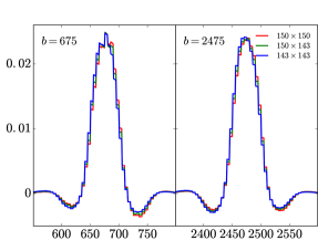
Figure 3.— The window functions $W_{b\ell}$ for the $D_{b}^{150\times 150}$ (red), $D_{b}^{150\times 143}$ (green), and $D_{b}^{143\times 143}$ (blue) bandpowers, for bins centered at $\ell=675$ and $2475$. In both panels, $W_{b\ell}^{143\times 143}$ has a higher (lower) weight on $\ell$s lower (higher) than the bin center of $W_{b\ell}^{150\times 150}$, and $W_{b\ell}^{150\times 143}$ sits between the two. Due to the shape of CMB power spectrum, $D_{\ell}$, such difference leads to an $\ell$-dependent bias when directly comparing the three sets of bandpowers.

To characterize the level of consistency between the three sets of bandpowers ($150\times 150$, $150\times 143$, and $143\times 143$), we choose one set, $D_{b}^{150\times 150}$, as the fiducial which is subtracted from or divided into the other two sets (see Section 4.2). However, the residual bandpowers and bandpower ratios are biased due to the difference of bandpower window functions (e.g., Knox, 1999). Due to the different filtering and the beam transfer functions of the two experiments, the bandpower window functions are different between bandpower sets. In Figure 3, the window functions of the three sets of bandpowers are illustrated for two bins with effective centers at $\ell=675$ and $\ell=2475$. In both of these bins, relative to the $150\times 150$ window functions, the $143\times 143$ and $150\times 143$ bandpowers receive more weight from multipoles lower than the bin center and less from multipoles higher than the bin center. These differences, if left unaddressed, lead to a bias in the bandpower differences that is dependent, to some degree, on the assumed cosmological model.

Before comparing the bandpower sets, we need to correct for this bias. The correction is calculated as follows

$$\delta D^{i}_{b}=\sum_{\ell}(W^{i}_{\ell}-W^{150\times 150}_{\ell})D^{\rm fid}_{\ell}$$ (10)

where $i=150\times 143$, or $143\times 143$. The Planck 2015 best-fit cosmology plus the best-fit extra-galactic foregrounds are used as the fiducial model. We subtract this correction term from the $150\times 143$ and $143\times 143$ bandpowers to remove the bias caused by the bandpower window function differences. In Figure 4, the upper panel shows the shape of the correction $\delta D_{b}$ and the lower panel shows the ratio between $\delta D_{b}$ and the corresponding $D_{b}$. For $150\times 143$, $\delta D_{b}$ yields a roughly flat $1\%-2\%$ correction to the bandpower; while for $143\times 143$, the correction is more important at higher multipoles, up to $\sim 15\%$ at $\ell=2500$. The window function correction is clearly critical for the consistency analysis between these three sets of bandpowers.

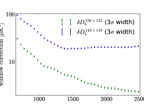
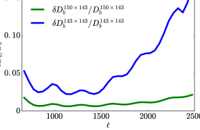
Figure 4.— Upper panel: The bandpower window function correction as given by Eq. 10 for $150\times 143$ (green) and $143\times 143$ (blue), with the fiducial $D_{\ell}$ including the Planck 2015 best-fit cosmology and the best-fit foreground models. The error bars indicate the $3\sigma$ variation in the window function corrections marginalized over a Markov chain based on WMAP9+SPT data. Lower panel: The ratio between the window function correction $\delta D_{b}^{i}$ and the corresponding bandpower $D_{b}^{i}$ for $i=150\times 143$ (green) and $143\times 143$ (blue).

We now investigate the model dependence of the window function corrections. To characterize this dependence, we calculate the window function corrections for a distribution of input $D_{\ell}$. The distribution is obtained by randomly sampling the cosmology and foreground models from a Markov chain based on WMAP9+SPT data. The variation of $\delta D_{b}$ in Eq. 10 is illustrated in the upper panel of Figure 4 with the error bars indicating the $3\sigma$ variation of the corrections. Within the band range of interest, this variation level is less than 1% of the bandpower standard error, we therefore ignore this very small uncertainty in our analysis.

4. Results

In this section, we present the results of the comparison between SPT 150 GHz data and Planck 143 GHz data. We first present a qualitative map-level comparison of the two data sets in a common sky area. We then present the major result of the paper: the bandpower comparison among three sets of bandpowers calculated on the 2540 $\text{deg}^{2}$ SPT-SZ sky patch: $\mathcal{D}_{b}^{150\times 150}$, $\mathcal{D}_{b}^{150\times 143}$, and $\mathcal{D}_{b}^{143\times 143}$. Setting $\mathcal{D}_{b}^{150\times 150}$ as the fiducial and subtracting it from the other two, we use the residual as the quantity to characterize the level of consistency between SPT 150 GHz and Planck 143 GHz data. As a byproduct, for the first time we recalibrate the SPT data to the Planck data on the same patch of sky.

We also characterize the ratios between these sets of bandpowers. Note that the residual and ratio tests are not intended to be independent checks, as they contain nearly the same information presented in different ways. The reason we use both metrics is that the systematic errors most likely to cause differences between SPT and Planck data (such as unmodeled foreground residuals or beam systematics) fall into two broad categories: additive or multiplicative systematics. Additive systematics will show up most obviously in the residual bandpower test, while multiplicative systematics will show up most obviously in a bandpower ratio test.

Finally, we compare each set of 2540 $\text{deg}^{2}$ bandpowers to the full-sky Planck 143 GHz bandpowers. Obviously such bandpower comparisons are not distinct from the map comparison. Rather, the residuals and the ratios of these sets of bandpowers are the quantitative version of the by-eye map comparison.

4.1. Map-level Comparison

The SPT and Planck maps within the same patch are presented in Figure 5 for visual comparison. The upper panels show the filtered SPT map described in Section 2.1 on the left and the projected Planck full-mission 143 GHz map on the right. Some bright point sources can be identified by eye in both the SPT and Planck maps, but the maps do not resemble each other, because the Planck map is dominated by the degree-scale CMB anisotropy filtered out of the SPT data, and the SPT map shows more small-scale structure due to its higher angular resolution. In the lower panels of Figure 5, we show SPT and Planck maps of the same spatial modes. The lower-left panel shows the SPT map from the upper-left panel convolved with the difference between the SPT 150 GHz and Planck 143 GHz beams; the lower-right panel shows a map made by observing a Planck sky with the SPT 150 GHz scan strategy and TOD filtering. Though the Planck map has a visibly higher noise level (as expected), the signals in the two maps appear nearly identical. Figure 6 shows the difference between the lower-left and lower-right maps from Figure 5, on the same color scale, along with a simulated difference map for comparison. The feature at the location of one of the bright point sources is most likely caused by temporal variability of the source, as the SPT and Planck data were not taken simultaneously.

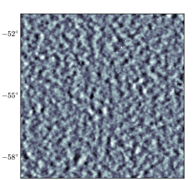
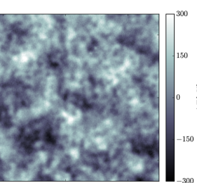
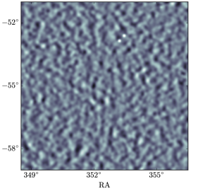
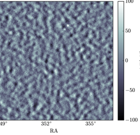
Figure 5.— Temperature maps of a portion of one SPT-SZ survey field. Upper left: the SPT-SZ 150 GHz map of this region. Modes with $\ell\lesssim 600$ are strongly suppressed in this map by the high-pass filter applied to the time-ordered data. Upper right: the Planck 143 GHz full-mission map of the same area. Lower left: the SPT map from the upper-left panel smoothed to have the same resolution as the Planck map. Lower right: the Planck map from the upper-right panel with the SPT-SZ high-pass filter applied. The difference between the lower-left and lower-right panels is shown in Figure 6. Note: the grayscale range of the top right panel is $[-300\mathrm{\mu K},\mathrm{300\mu K}]$, and the greyscale range of the other three panels is $[-100\mathrm{\mu K},\mathrm{100\mu K}]$.

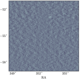
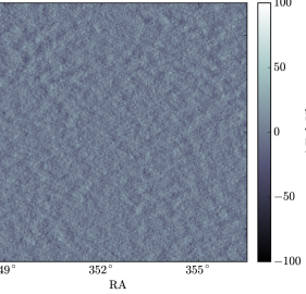
Figure 6.— Left panel: The residual map between the smoothed SPT-SZ 150 GHz map in the lower-left panel of Figure 5 and the high-pass-filtered Planck 143 GHz map in the lower-right panel of Figure 5. The feature at the location of one of the bright point sources is potentially due to temporal variability of the source, as the SPT and Planck data were not taken simultaneously. Right panel: Same as left panel, but with simulated data, consisting of the sum of an SPT-SZ noise realization smoothed to match Planck resolution and a Planck noise realization filtered to match the time-domain filtering of the SPT-SZ data.

To make this result more quantitative, we could match the beam and filtering between these two data sets over the full SPT-SZ survey region, mask point sources, calculate the power in the difference map, and compare that power to the expected power from noise alone. In the next section we do a nearly equivalent but somewhat simpler calculation. Using the cross-spectrum formalism outlined in Section 3, we calculate the Planck $143\times 143$ power spectrum, the SPT $150\times 150$ power spectrum, and the SPT-Planck $150\times 143$ cross-spectrum, and we calculate the $\chi^{2}$ of the null hypothesis that these three spectra are measuring the same power. This calculation does not completely eliminate sample variance, as the perfectly mode-matched difference-map power spectrum would, but it strongly reduces it (see Figure 8).

4.2. Bandpower Comparison and Recalibration

In this section, we present the comparison between the three sets of window-function-corrected bandpowers, which we denote as $\mathcal{D}_{b}^{150\times 150}$, $\mathcal{D}_{b}^{150\times 143}$, and $\mathcal{D}_{b}^{143\times 143}$. We first show all three sets of bandpowers in the upper panel of Figure 7. The error bars contain contributions from sample variance, noise variance, and beam uncertainties. By eye, the three sets of bandpowers look very consistent. At low $\ell$, the scatter among the three sets of points is much smaller than the errors on any one set; this is because the errors on all three are dominated by sample variance in this regime, and sample variance is highly correlated among the three data sets. This is also why the three sets of error bars are nearly the same size at low $\ell$ (though the $143\times 143$ bandpowers have slightly smaller error bars in this $\ell$ range because the modes lost in the SPT TOD filtering process result in slightly increased sample variance). Noise variance begins to dominate the $143\times 143$ error bars at $\ell\gtrsim 1700$ and the $150\times 143$ error bars at $\ell\gtrsim 2000$, while the $150\times 150$ error bars are sample-variance-dominated over the entire range plotted.

The remaining panels of Figure 7 show various comparisons among the three sets of bandpowers. Two comparison schemes are applied: differences and ratios. The former is good for diagnosing additive effects, while the latter is more sensitive to multiplicative systematics. In both schemes, $\mathcal{D}_{b}^{150\times 150}$ is chosen as the fiducial bandpower set. These comparison plots and the $\chi^{2}$ and the probability to exceed (PTE) statistics calculated below are thus testing the following set of null hypotheses: 1) two sets of bandpower residuals

$$\langle\Delta\mathcal{D}_{b,c}\rangle \equiv \langle\mathcal{D}_{b}^{150\times 143}-\mathcal{D}_{b}^{150\times 150}\rangle=0$$

$$\langle\Delta\mathcal{D}_{b,a}\rangle \equiv \langle\mathcal{D}_{b}^{143\times 143}-\mathcal{D}_{b}^{150\times 150}\rangle=0$$

and 2) two sets of bandpower ratios

$$\langle\Delta\mathcal{D}_{b,c}/\mathcal{D}_{b}^{150\times 150}\rangle \equiv \langle\mathcal{D}_{b}^{150\times 143}/\mathcal{D}_{b}^{150\times 150}\rangle-1=0$$

$$\langle\Delta\mathcal{D}_{b,a}/\mathcal{D}_{b}^{150\times 150}\rangle \equiv \langle\mathcal{D}_{b}^{143\times 143}/\mathcal{D}_{b}^{150\times 150}\rangle-1=0.$$

The absolute calibration of the SPT data from George et al. (2015) has a statistical uncertainty of $\sim$1% at 150 GHz. We expect the bandpower comparison to be significantly more precise than this, so before plotting the bandpower residuals and ratios and before testing the null hypotheses above, we apply a recalibration parameter $r_{c}$ to bandpowers containing SPT data:

$$\Delta\mathcal{D}_{b,c} \equiv r_{c}\mathcal{D}_{b}^{150\times 143}-r_{c}^{2}\mathcal{D}_{b}^{150\times 150}$$ (11)

$$\Delta\mathcal{D}_{b,a} \equiv \mathcal{D}_{b}^{143\times 143}-r_{c}^{2}\mathcal{D}_{b}^{150\times 150},$$ (12)

and similarly for the bandpower ratios. Because of the precision of the George et al. (2015) calibration, we expect $r_{c}$ to be very close to 1. We then calculate and minimize $\chi^{2}$ as a function of $r_{c}$:

$$\chi^{2}(r_{c})=\Delta\mathbf{D}^{T}_{\mathrm{b}}(r_{c})\Xi^{-1}\Delta\mathbf{D}_{\mathrm{b}}(r_{c}),$$ (13)

and similarly for the bandpower ratios, where $\Delta\mathbf{D}_{\mathrm{b}}$ denotes the vector that includes both $\Delta\mathcal{D}_{b,c}$ and $\Delta\mathcal{D}_{b,a}$. We fit the two sets of residuals or ratios simultaneously. In principle we should include the recalibration parameter in an adjustment to the noise contribution to the covariance matrix, but we neglect it for simplicity, with the justification that the correction is very small at less than 1%. In Figure 7, we have included the best-fit recalibration parameter for SPT, $r_{c}$, in all three panels.

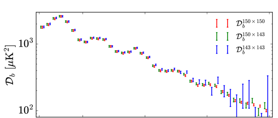
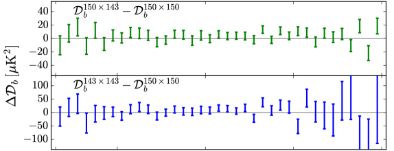
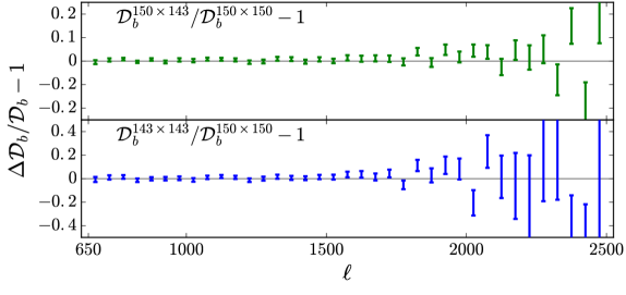
Figure 7.— Upper panel: The window-function-corrected, unbiased bandpowers for $150\times 150$ (red), $150\times 143$ (green), and $143\times 143$ (blue). The error bars contain sample variance and noise variance obtained from our simulations, as well as beam uncertainties from the analytical calculations presented in Section 3.4.2. The green and blue error bars are offset horizontally for clarity. Middle panel: The bandpower residuals $\mathcal{D}_{b}^{150\times 143}-\mathcal{D}_{b}^{150\times 150}$ (green) and $\mathcal{D}_{b}^{143\times 143}-\mathcal{D}_{b}^{150\times 150}$ (blue) with the window function correction. The error bars come from the diagonal of the covariance matrix of the bandpower residuals of Eq. 3.4.2. Under our null hypothesis, the residuals are expected to be consistent with 0. Note the different plotting range between the two bandpower residuals. Lower panel: The window-function-corrected bandpower ratios $\mathcal{D}_{b}^{150\times 143}/\mathcal{D}_{b}^{150\times 150}-1$ (green) and $\mathcal{D}_{b}^{143\times 143}/\mathcal{D}_{b}^{150\times 150}-1$ (blue). The best-fit recalibration parameter for SPT, $r_{c}$, has been applied to all panels of this figure.

In the middle panel of Figure 7 we show the bandpower residuals $\Delta\mathcal{D}_{b,c}$ and $\Delta\mathcal{D}_{b,a}$ with error bars given by the square root of the diagonal elements of the full covariance matrix. This figure shows the residual bandpowers are consistent with zero given the errors. In the lower panels of the same figure we show the bandpower ratios. Similar to the residuals, the error bars of the bandpower ratios are the square root of the diagonal elements of the full covariance matrix. Qualitively, these results appear to be consistent with our null hypotheses.

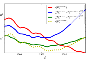
Figure 8.— Uncertainties in the SPT $150\times 150$ bandpowers (red) and in the two sets of bandpower residuals (not including beam uncertainty). The sample variance is significantly reduced in the $150\times 150-143\times 143$ residuals compared to the $150\times 150$ bandpowers (by roughly a factor of six in the lowest $\ell$ ranges, and by a larger factor at higher $\ell$), indicating that this comparison is more stringent than the comparison of $150\times 150$ to full-sky Planck data, the uncertainty on which is dominated by the sample variance in the $150\times 150$ spectrum. Also plotted are the bandpower uncertainties from full-sky Planck data, scaled to the $\ell$ bin size used in this work.

Table 1Best-fit recalibration parameter, $\chi^{2}$, and PTE for the various bandpower comparisons.

Comparison	best $r_{c}$	$\chi^{2}$	PTE
Residual, combined, full covariance	$1.0087\pm 0.0015$	78.7	0.30
Residual, combined, no beam error	$1.0117\pm 0.0009$	89.8	0.09
$150\times 143-150\times 150$, full covariance	$1.0087\pm 0.0016$	42.1	0.22
$150\times 143-150\times 150$, no beam error	$1.0115\pm 0.0010$	50.4	0.06
$143\times 143-150\times 150$, full covariance	$1.0076\pm 0.0022$	36.8	0.43
$143\times 143-150\times 150$, no beam error	$1.0110\pm 0.0013$	41.8	0.23
Ratio, combined, full covariance	$1.0092\pm 0.0015$	81.0	0.24
Ratio, combined, no beam error	$1.0120\pm 0.0009$	91.0	0.08
$(150\times 143)/(150\times 150)$, full covariance	$1.0090\pm 0.0016$	43.3	0.19
$(150\times 143)/(150\times 150)$, no beam error	$1.0118\pm 0.0010$	50.9	0.05
$(143\times 143)/(150\times 150)$, full covariance	$1.0082\pm 0.0022$	38.1	0.37
$(143\times 143)/(150\times 150)$, no beam error	$1.0113\pm 0.0013$	42.4	0.21

The quantitative characterization comes from the $\chi^{2}$ value with the best-fit recalibration parameter. The best-fit values of $r_{c}$, minimum $\chi^{2}$, and probabilities to exceed that $\chi^{2}$ are listed in Table 1 for several combinations of data and covariance. The primary results are from the combined residual bandpowers. Using the full $2\times 2$-block covariance matrix for the recalibration fit, these results give a best-fit of $r_{c}=1.0087\pm 0.0015$ with $\chi^{2}=78.7$. There are 37 $\ell$ bins in our analysis, so we have 74 data points among the two residual bandpowers and one free parameter. The PTE for $\chi^{2}=78.7$ and 73 degrees of freedom is 0.30. We find very similar results from the combined-ratio fit: $r_{c}=1.0092\pm 0.0015$, $\chi^{2}=81.02$, $\mathrm{PTE}=0.24$. Put another way, given the noise properties and the beam uncertainties of the two experiments, 30% (24%) of our simulations have a higher $\chi^{2}$ for the bandpower differences (ratios) than we find with the real data. We thus find as our primary result that the SPT and Planck data in the SPT-SZ sky patch are quite consistent with the null hypothesis that there is no systematic offset in the two experiments’ measurement of the sky. A byproduct of this analysis is that we recalibrate the SPT data with a statistical precision of 0.30% in power (0.15% in temperature) relative to Planck 143 GHz. This is comparable with the absolute calibration uncertainty of the Planck 143 GHz, 0.14% in power (0.07% in temperature, Planck Collaboration et al. 2016b), so we add this uncertainty in quadrature for a final SPT 150 GHz calibration uncertainty of 0.33% in power.

In Table 1, we also report the quantities of consistency from the single pair of bandpowers. For example, the PTE is 0.22 for the residual between $\mathcal{D}_{b}^{150\times 143}$ and $\mathcal{D}_{b}^{150\times 150}$ with the full covariance matrix. For the other pair of residual bandpowers, $\mathcal{D}_{b}^{143\times 143}$ and $\mathcal{D}_{b}^{150\times 150}$, the PTE is 0.43 with the full covariance matrix. The results without the beam uncertainties are also listed in Table 1.

As discussed in Section 3.2.2, the white-noise assumption in simulations for $\mathcal{D}_{b}^{143\times 143}$ results in an overestimate of the noise contribution to the covariance matrix, at roughly the 10% level in $\mathcal{D}_{b}$ errors, or the 20% level in variance. If we assumed the Planck noise was the dominant contribution to the residual and ratio covariance in the $150\times 150$ vs. $143\times 143$ comparisons, we would expect roughly a 20% increase in $\chi^{2}$ if we were able to use more realistic noise simulations. The resulting $\chi^{2}$ would still correspond to a reasonable PTE ($\gtrsim 0.16$) for the null hypothesis. This would also be true of the combined constraints, particularly because the main constraining power comes from $\mathcal{D}_{b}^{150\times 143}$, which is unaffected by the assumption of white noise in the Planck-only bandpowers.

Because of the largely reduced sample variance contribution to the difference between bandpowers within the same sky coverage (roughly a factor of six in $150\times 143-150\times 150$ compared to $150\times 150$), the comparison of $\mathcal{D}_{b}^{150\times 150}$ with the $\mathcal{D}_{b}^{150\times 143}$ and $\mathcal{D}_{b}^{143\times 143}$ bandpowers derived from within the SPT patch, provide tighter tests, over a wide range of angular scales, than can be achieved by the comparison of $\mathcal{D}_{b}^{150\times 150}$ with the more precise Planck spectra derived from nearly the full sky. In Figure 8, we compare the uncertainties on the two sets of bandpower residuals $\mathcal{D}_{b}^{143\times 143}-\mathcal{D}_{b}^{150\times 150}$ (blue), and $\mathcal{D}_{b}^{150\times 143}-\mathcal{D}_{b}^{150\times 150}$ (green) to the uncertainties on the SPT-only bandpowers $\mathcal{D}_{b}^{150\times 150}$ (red). In the lower-$\ell$ region ($\ell<1800$), the green curve has the lowest error because the sample variance has been greatly reduced by subtracting the SPT bandpowers from the cross bandpowers, while at higher $\ell$ the green curve rises due to the Planck noise contribution. In the most constraining case ($\mathcal{D}_{b}^{150\times 143}-\mathcal{D}_{b}^{150\times 150}$), the errors for almost all bins are $\leq 10\mathrm{\mu K^{2}}$, comparable to the uncertainty in the PlanckFS bandpowers. Both sets of bandpower residuals yield very stringent tests on the consistency of the two datasets, and our results show that these datasets are formally consistent in this patch.

4.3. Comparison to the Full-sky Planck 2015 TT High-$\ell$ Bandpowers

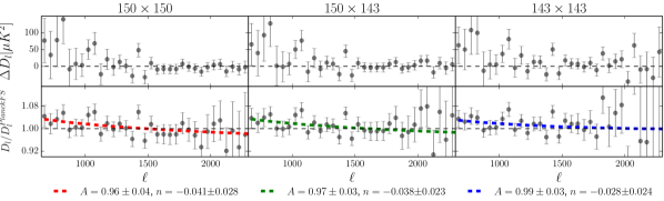
Figure 9.— Upper panel: Residuals between the in-patch and PlanckFS bandpowers. Lower panel: Ratios of the in-patch and PlanckFS bandpowers. The colored dashed lines are the best-fit power laws for each ratio.

While restricting the bandpower comparison to overlapping sky substantially reduces differential sample variance, it does increase the Planck covariance. In this section, we instead investigate differences between the “in-patch” bandpowers (i.e., the 150 $\times$ 150, 150 $\times$ 143, and 143 $\times$ 143 bandpowers from the 2540 deg² SPT-SZ survey region) and the full-sky Planck 2015 TT high-$\ell$ unbinned frequency combined bandpowers (Planck Collaboration et al., 2016e), which we refer to as “PlanckFS.” In this case, the null hypothesis is that any differences between PlanckFS and the in-patch bandpowers are consistent with expectations given Gaussian statistics and statistical isotropy.

In Figure 9 we show the residuals and ratios for the in-patch to PlanckFS bandpowers. The residual plots show all three sets of the in-patch bandpowers prefer greater power at $650<\ell<1200$, indicating the SPT-SZ patch has greater power at these multipoles than the full-sky average. The ratio plots also suggest a tilt with respect to PlanckFS, although the significance is modest. The slope of the tilt is consistent to $0.5\,\sigma$ between the three cross-spectra, being slightly larger in $150\times 150$ and smaller in $143\times 143$.

To quantify the statistical significance of this tilt we model the ratio of the in-patch and PlanckFS bandpowers as a power law:

$$\frac{D^{th,i\times j}_{\ell}}{D^{\rm{PlanckFS}}_{\ell}}=A\left(\frac{\ell}{4000}\right)^{n}.$$ (14)

We assume a Gaussian likelihood with

$$-2\ln\mathcal{L}(A,n|D^{i\times j},D^{\mathrm{PlanckFS}})=\Delta_{b}\Sigma_{bb^{\prime}}^{-1}\Delta_{b}^{\prime},$$ (15)

$$\Delta_{b}=\frac{D^{i\times j}_{b}}{W^{i\times j}_{b\ell}D^{\mathrm{PlanckFS}}_{\ell}}-R_{b}^{i\times j}(A,n),$$ (16)

$$R_{b}^{i\times j}(A,n)=W^{i\times j}_{b\ell}\bigg{(}A\bigg{(}\frac{\ell}{4000}\bigg{)}^{n}+F^{i\times j}_{\ell}\bigg{)}.$$ (17)

Here $D^{\mathrm{PlanckFS}}_{\ell}$ is the best-fit PlanckFS power spectrum, $\Sigma_{bb^{\prime}}=\langle\Delta_{b}\Delta_{b^{\prime}}\rangle$ (only the SPT beam uncertainty is included and cross-correlations between $D^{i\times j}_{b}$ and the $D^{\mathrm{PlanckFS}}_{\ell}$ are negligible), and $F^{i\times j}_{\ell}$ is the foreground model adopted from S13 with the frequency dependence from George et al. (2015) included. There are three foreground amplitude parameters included in $F^{i\times j}_{\ell}$ to account for the SZ, Poisson-point-source, and clustered CIB uncertainties. The best-fit re-calibration from Section 4.3 has been applied to the in-patch SPT-only and SPT-Planck bandpowers. The best-fit values for $A$ and $n$ are reported in Figure 9. We find only marginal evidence for a tilt between PlanckFS and any of the three cross-spectra; the most significant tilt is for $150\times 150$ and is $1.5\,\sigma$ away from zero. We conclude that the tilts we see in the observed spectra are roughly consistent with the expectation based on Gaussian statistics and the assumption of statistical isotropy—i.e., they are roughly consistent with $n=0$.

Table 2Power-law Parameter PTEs

	$\chi^{2}$	PTE
$150\times 150-150\times 143$	0.33	0.41
$150\times 150-143\times 143$	1.79	0.85
$150\times 143-143\times 143$	1.18	0.55

• The $\chi^{2}$ and PTE for the null hypothesis that the
  tilt relative to PlanckFS is the same in the in-patch
  $150\times 150$, $150\times 143$, and $143\times 143$ bandpowers.

To determine the expected statistical properties of the differences in the best-fit values of $A$ and $n$ we construct a covariance matrix ($\mathbf{C}$) from the set of best-fit values of $A$ and $n$ in each of the 400 simulations of Section 3.2. We then calculate $\chi^{2}$ for these differences as

$$\chi^{2}=(\mathbf{\Theta}-\bar{\mathbf{\Theta}})^{\intercal}\mathbf{C}^{-1}(\mathbf{\Theta}-\bar{\mathbf{\Theta}})$$ (18)

where $\mathbf{\Theta}$ is the vector of parameter differences and $\bar{\mathbf{\Theta}}$ is the mean simulation difference, which is consistent with zero. The breakdown of PTEs for the various pair differences is shown in Table 2. As can be seen, the most extreme PTE is 0.85 and the lowest is 0.41. We conclude that the observed tilts in the three cross-spectra are completely consistent with each other.

All our tests are consistent with the following explanation for the tilts we observe in the in-patch spectra relative to the best-fit Planck full-sky spectrum: they are driven by a sample-variance fluctuation away from the full-sky average, the magnitude of which is roughly consistent with expectations under the assumption of statistical isotropy and our noise model.

4.4. Pipeline Checks

All published power spectra from the SPT collaboration have been calculated using some variant of the cross-spectrum pseudo-$C_{\ell}$ pipeline used in this work. Extensive checks have been performed on this pipeline (see, e.g., Section 4.2 of Story et al. 2013), demonstrating that the correct input spectrum is recovered from simulated data, even when that spectrum differs from the spectrum assumed in calculating the filter transfer function. If, however, some aspect of the pipeline were inducing a bias in the estimated power spectra (through some mechanism that has escaped all pipeline tests), this bias would affect both the SPT-SZ and Planck data used in this work (because we have mock-observed the Planck data and analyzed it with the SPT pipeline). If the bias on the two data sets were comparable, it would then divide or subtract out in the bandpower comparison, and we would (wrongly) conclude there was no issue with either data set.

To test this scenario, we have analyzed the in-patch Planck data using an alternate pipeline. Specifically, we created a HEALPix version of the SPT-SZ sky-patch and point-source mask (stitched together from the individual-field masks), and we handed this mask and the half-mission Planck 143 GHz maps to the PolSpice(Szapudi et al., 2001; Chon et al., 2004) code, which is designed to estimate the power spectra of masked full-sky maps and properly account for the masking. We binned the $\Delta\ell=1$ PolSpice output into the $\Delta\ell=50$ bins used in the SPT pipeline using the bandpower window functions calculated for the $143\times 143$ “scanned, filtered” Planck bandpowers. We then calculated the ratio of the “unscanned, unfiltered” (PolSpice) bandpowers to the scanned, filtered ones and found that they agree to better than 3% in every individual bin in which there is appreciable signal-to-noise in the $143\times 143$ spectrum, with an overall ratio of $1.0028\pm 0.0050$ over the range $600<\ell<1800$ and no evidence of a trend with $\ell$. We have also re-done the tilt calculation in Section 4.3 using the unscanned, unfiltered bandpowers and found results consistent with what we found with the scanned, filtered bandpowers (within a fraction of a sigma). We thus conclude that our fundamental results are not an artifact of the SPT analysis method.

5. Conclusions

In this paper, we have compared 150 GHz SPT data and 143 GHz Planck data in the same region of the sky, namely the 2540 $\deg^{2}$ SPT-SZ survey footprint. We have performed a visual comparison of maps constructed from the two data sets and found the difference between the two maps to be visually consistent with noise, once they have been filtered to display the same angular modes.

We then performed a quantitative analysis of the consistency of the maps, relying primarily on a comparison of the cross-spectrum of two halves of the SPT data with the SPT $\times$ Planck cross spectrum. We also compared the SPT $\times$ SPT spectrum with the cross-spectrum of two halves of the Planck data. These comparisons were made using differences between and ratios of two sets of binned power spectra, or bandpowers, at a time, always using the SPT $\times$ SPT bandpowers as the fiducial set. To test the null hypothesis that the bandpower differences (after recalibrating the SPT data) are consistent with zero—or that the ratios are consistent with unity—we created a suite of 400 simulations of the signal and noise properties of the SPT and Planck maps, including signal contributions from the CMB and extragalactic foregrounds. We found our most stringent test, based on the expected variance of the differences, to be the comparison of the SPT $\times$ SPT spectrum with the SPT-Planck cross spectrum. Forming a $\chi^{2}$ quantity from these bandpower differences and the simulation-based covariance matrix, we have found a value that is exceeded by 22% of the analogous $\chi^{2}$ values derived from the simulated data, i.e., corresponding to the PTE value 0.22. When we add the residuals between the SPT $\times$ SPT and Planck $\times$ Planck cross-spectra, we find a PTE of 30%. All other tests result in similarly unremarkable PTEs. We find no evidence of a failure of our null model; i.e., we see no evidence for systematic errors or under- or over-estimate of statistical errors.

We have also compared the three sets of bandpowers from the 2540 deg² SPT-SZ survey region to the full-sky Planck 143 GHz power spectrum. Relative to the Planck full-sky spectrum, we have found a hint for a tilt in the in-patch bandpowers. For all three sets of in-patch bandpowers, the amplitude of the tilts we have obtained are consistent with each other and roughly consistent with expected noise and sample variance fluctuations.

This work shows that the SPT 150 GHz and Planck 143 GHz data are in very good agreement with each other within the 2540 deg² SPT-SZ survey area. In a companion paper (Aylor et al., 2017), we extend this comparison to the cosmological parameters that can be derived from these bandpowers.

References

- Addison et al. (2016) Addison, G. E., Huang, Y., Watts, D. J., et al. 2016, ApJ, 818, 132
- Aylor et al. (2017) Aylor, K., Hou, Z., Knox, L., et al. 2017, ApJ, 850, 101
- Battye & Moss (2014) Battye, R. A., & Moss, A. 2014, Physical Review Letters, 112, 051303
- Bennett et al. (2013) Bennett, C. L., Larson, D., Weiland, J. L., et al. 2013, ApJS, 208, 20
- Cai et al. (2013) Cai, Z.-Y., Lapi, A., Xia, J.-Q., et al. 2013, ApJ, 768, 21
- Calabrese et al. (2013) Calabrese, E., Hlozek, R. A., Battaglia, N., et al. 2013, Phys. Rev. D, 87, 103012
- Chon et al. (2004) Chon, G., Challinor, A., Prunet, S., Hivon, E., & Szapudi, I. 2004, MNRAS, 350, 914
- De Zotti et al. (2005) De Zotti, G., Ricci, R., Mesa, D., et al. 2005, A&A, 431, 893
- Efstathiou et al. (2014) Efstathiou, A., Pearson, C., Farrah, D., et al. 2014, MNRAS, 437, L16
- George et al. (2015) George, E. M., Reichardt, C. L., Aird, K. A., et al. 2015, ApJ, 799, 177
- Górski et al. (2005) Górski, K. M., Hivon, E., Banday, A. J., et al. 2005, ApJ, 622, 759
- Hinshaw et al. (2013) Hinshaw, G., Larson, D., Komatsu, E., et al. 2013, ApJS, 208, 19
- Hivon et al. (2002) Hivon, E., Górski, K. M., Netterfield, C. B., et al. 2002, ApJ, 567, 2
- Hou et al. (2014) Hou, Z., Reichardt, C. L., Story, K. T., et al. 2014, ApJ, 782, 74
- Keisler et al. (2011) Keisler, R., Reichardt, C. L., Aird, K. A., et al. 2011, ApJ, 743, 28
- Knox (1999) Knox, L. 1999, Phys. Rev. D, 60, 103516
- Lewis (2005) Lewis, A. 2005, Phys. Rev. D, 71, 083008
- Louis et al. (2014) Louis, T., Addison, G. E., Hasselfield, M., et al. 2014, J. of Cosm. & Astropart. Phys., 7, 016
- Mocanu et al. (2013) Mocanu, L. M., Crawford, T. M., Vieira, J. D., et al. 2013, ApJ, 779, 61
- Planck Collaboration et al. (2014a) Planck Collaboration, Ade, P. A. R., Aghanim, N., et al. 2014a, A&A, 571, A1
- Planck Collaboration et al. (2014b) —. 2014b, A&A, 571, A7
- Planck Collaboration et al. (2014c) —. 2014c, A&A, 571, A16
- Planck Collaboration et al. (2016a) Planck Collaboration, Adam, R., Ade, P. A. R., et al. 2016a, A&A, 594, A7
- Planck Collaboration et al. (2016b) —. 2016b, A&A, 594, A8
- Planck Collaboration et al. (2016c) Planck Collaboration, Aghanim, N., Arnaud, M., et al. 2016c, A&A, 594, A11
- Planck Collaboration et al. (2016d) Planck Collaboration, Ade, P. A. R., Aghanim, N., et al. 2016d, A&A, 594, A12
- Planck Collaboration et al. (2016e) —. 2016e, A&A, 594, A13
- Planck Collaboration et al. (2016f) —. 2016f, A&A, 594, A24
- Planck Collaboration et al. (2017) Planck Collaboration, Aghanim, N., Akrami, Y., et al. 2017, A&A, 607, A95
- Riess et al. (2011) Riess, A. G., Macri, L., Casertano, S., et al. 2011, ApJ, 730, 119
- Riess et al. (2016) Riess, A. G., Macri, L. M., Hoffmann, S. L., et al. 2016, ApJ, 826, 56
- Schaffer et al. (2011) Schaffer, K. K., Crawford, T. M., Aird, K. A., et al. 2011, ApJ, 743, 90
- Shaw et al. (2010) Shaw, L. D., Nagai, D., Bhattacharya, S., & Lau, E. T. 2010, ApJ, 725, 1452
- Shaw et al. (2012) Shaw, L. D., Rudd, D. H., & Nagai, D. 2012, ApJ, 756, 15
- Snyder (1987) Snyder, J. P. 1987, Map projections–a working manual (Washington: U.S. Geological Survey)
- Story et al. (2013) Story, K. T., Reichardt, C. L., Hou, Z., et al. 2013, ApJ, 779, 86
- Szapudi et al. (2001) Szapudi, I., Prunet, S., Pogosyan, D., Szalay, A. S., & Bond, J. R. 2001, ApJ, 548, L115
- Wyman et al. (2014) Wyman, M., Rudd, D. H., Vanderveld, R. A., & Hu, W. 2014, Physical Review Letters, 112, 051302