Estimating the spectral gap of a trace-class Markov operator

Abstract

The utility of a Markov chain Monte Carlo algorithm is, in large part, determined by the size of the spectral gap of the corresponding Markov operator. However, calculating (and even approximating) the spectral gaps of practical Monte Carlo Markov chains in statistics has proven to be an extremely difficult and often insurmountable task, especially when these chains move on continuous state spaces. In this paper, a method for accurate estimation of the spectral gap is developed for general state space Markov chains whose operators are non-negative and trace-class. The method is based on the fact that the second largest eigenvalue (and hence the spectral gap) of such operators can be bounded above and below by simple functions of the power sums of the eigenvalues. These power sums often have nice integral representations. A classical Monte Carlo method is proposed to estimate these integrals, and a simple sufficient condition for finite variance is provided. This leads to asymptotically valid confidence intervals for the second largest eigenvalue (and the spectral gap) of the Markov operator. In contrast with previously existing techniques, our method is not based on a near-stationary version of the Markov chain, which, paradoxically, cannot be obtained in a principled manner without bounds on the spectral gap. On the other hand, it can be quite expensive from a computational standpoint. The efficiency of the method is studied both theoretically and empirically.

1 Introduction

Markov chain Monte Carlo (MCMC) is widely used to estimate intractable integrals that represent expectations with respect to complicated probability distributions. Let $\pi:S\to[0,\infty)$ be a probability density function (pdf) with respect to a $\sigma$-finite measure $\mu$, where $(S,\mathcal{U},\mu)$ is some measure space. Suppose we want to approximate the integral

$$J:=\int_{S}f(u)\pi(u)\mu(du)$$

for some function $f:S\to\mathbb{R}$. Then $J$ can be estimated by $\hat{J}_{m}:=m^{-1}\sum_{k=0}^{m-1}f(\Phi_{k}),$ where $\{\Phi_{k}\}_{k=0}^{m-1}$ are the first $m$ elements of a well-behaved Markov chain with stationary density $\pi(\cdot)$. Unlike classical Monte Carlo estimators, $\hat{J}_{m}$ is not based on iid random elements. Indeed, the elements of the chain are typically neither identically distributed nor independent. Given $\mathrm{var}_{\pi}f,$ the variance of $f(\cdot)$ under the stationary distribution, the accuracy of $\hat{J}_{m}$ is primarily determined by two factors: (i) the convergence rate of the Markov chain, and (ii) the correlation between the $f(\Phi_{k})$s when the chain is stationary. These two factors are related, and can be analyzed jointly under an operator theoretic framework.

The starting point of the operator theoretic approach is the Hilbert space of functions that are square integrable with respect to the target pdf, $\pi(\cdot)$. The Markov transition function that gives rise to $\Phi=\{\Phi_{k}\}_{k=0}^{\infty}$ defines a linear (Markov) operator on this Hilbert space. (Formal definitions are given in Section 2.) If $\Phi$ is reversible, then it is geometrically ergodic if and only if the corresponding Markov operator admits a positive spectral gap (Roberts and Rosenthal, 1997; Kontoyiannis and Meyn, 2012). The gap, which is a real number in $(0,1]$, plays a fundamental role in determining the mixing properties of the Markov chain, with larger values corresponding to better performance. For instance, suppose $\Phi_{0}$ has pdf $\pi_{0}(\cdot)$ such that $d\pi_{0}/d\pi$ is in the Hilbert space, and let $d(\Phi_{k};\pi)$ denote the total variation distance between the distribution of $\Phi_{k}$ and the chain’s stationary distribution. Then, if $\delta$ denotes the spectral gap, we have

$$d(\Phi_{k};\pi)\leq C(1-\delta)^{k}$$

for all positive integers $k,$ where $C$ depends on $\pi_{0}$ but not on $k$ (Roberts and Rosenthal, 1997). Furthermore, $(1-\delta)^{k}$ gives the maximal absolute correlation between $\Phi_{j}$ and $\Phi_{j+k}$ as $j\to\infty$. It follows (see e.g. Mira and Geyer, 1999) that the asymptotic variance of $\sqrt{m}(\hat{J}_{m}-J)$ as $m\to\infty$ is bounded above by

$$\frac{2-\delta}{\delta}\mathrm{var}_{\pi}f\,.$$

Unfortunately, it is impossible to calculate the spectral gaps of the Markov operators associated with practically relevant MCMC algorithms, and even accurately approximating these quantities has proven extremely difficult. In this paper, we develop a method of estimating the spectral gaps of Markov operators corresponding to a certain class of data augmentation (DA) algorithms (Tanner and Wong, 1987), and then show that the method can be extended to handle a much larger class of reversible MCMC algorithms.

DA Markov operators are necessarily non-negative. Moreover, any non-negative Markov operator that is compact has a pure eigenvalue spectrum that is contained in the set $[0,1]$, and $1-\delta$ is precisely the second largest eigenvalue. We propose a classical Monte Carlo estimator of $1-\delta$ for DA Markov operators that are trace-class, i.e. compact with summable eigenvalues. While compact operators were once thought to be rare in MCMC problems with uncountable state spaces (Chan and Geyer, 1994), a string of recent results suggests that trace-class DA Markov operators are not at all rare (see e.g. Qin and Hobert, 2018; Chakraborty and Khare, 2017; Choi and Román, 2017; Pal et al., 2017). Furthermore, by exploiting a simple trick, we are able to broaden the applicability of our method well beyond DA algorithms. Indeed, if a reversible Monte Carlo Markov chain has a Markov transition density (Mtd), and the corresponding Markov operator is Hilbert-Schmidt, then our method can be utilized to estimate its spectral gap. This is because the square of such a Markov operator can be represented as a trace-class DA Markov operator. A detailed explanation is provided in Section 4.

Of course, there is a large literature devoted to developing theoretical bounds on the second largest eigenvalue of a Markov operator (see e.g. Lawler and Sokal, 1988; Sinclair and Jerrum, 1989; Diaconis and Stroock, 1991). However, these results are typically not useful in situations where the state space, $S$, is uncountable or multi-dimensional, which is our main focus. There also exist a number of computational methods for approximating the eigenvalues of a Hilbert-Schmidt operator (see e.g. Garren and Smith, 2000; Koltchinskii and Giné, 2000; Ahues et al., 2001; Chakraborty and Khare, 2019+). Some such methods require sampling directly from $\pi(\cdot)$, which is impossible in an MCMC context. The others require the user to simulate the Markov chain of interest until it is nearly stationary. Unfortunately, we cannot know if a chain has converged unless we have some information on its convergence rate, which is essentially what these methods are trying to acquire in the first place. The classical Monte Carlo estimator that we introduce is calculated by simulating many copies of the Markov chain, each of a short length. These short chains need not be close to stationarity in order for the estimator to be valid. Although powerful, this method is quite expensive from a computational standpoint. Indeed, it works well only when the underlying dataset of the Bayesian model is small. On the other hand, it is important as a “proof of concept” that it is actually possible to get a handle on the spectral gaps of Markov operators corresponding to MCMC algorithms on continuous state spaces, which, until now, have proven to be extremely elusive quantities.

The rest of the paper is organized as follows. The notion of Markov operator is formalized in Section 2. In Section 3, it is shown that the second largest eigenvalue of a non-negative trace-class operator can be bounded above and below by functions of the power sums of the operator’s eigenvalues. In Section 4, DA Markov operators are formally defined, and the sum of the $k$th ($k\in\mathbb{N}$) power of the eigenvalues of a trace-class DA Markov operator is related to a functional of its Mtd. This functional is usually a multi-dimensional integral, and a classical Monte Carlo estimator of it is developed in Section 5. The efficiency of the Monte Carlo estimator is studied in Section 6. Finally, in Section 7 we apply our method to a few well-known MCMC algorithms. Our examples include Albert and Chib’s (1993) DA algorithm for Bayesian probit regression, and a DA algorithm for Bayesian linear regression with non-Gaussian errors (Liu, 1996). Further application of the method can be found in Zhang et al. (2019).

2 Markov operators

Assume that the Markov chain $\Phi$ has a Markov transition density, $p(u,\cdot),\,u\in S$, such that, for any measurable $A\subset S$ and $u\in S$,

$$\mathbb{P}(\Phi_{k}\in A|\Phi_{0}=u)=\int_{A}p^{(k)}(u,u^{\prime})\,\mu(du^{\prime})\,,$$

where

$$p^{(k)}(u,\cdot):=\left\{\begin{array}[]{@{}ll@{}}p(u,\cdot)&k=1\\ \int_{S}p^{(k-1)}(u,u^{\prime})p(u^{\prime},\cdot)\,\mu(du^{\prime})&k>1\end{array}\right.$$

is the $k$-step Mtd corresponding to $p(u,\cdot)$. We will assume throughout that $\Phi$ is Harris ergodic, i.e. irreducible, aperiodic and Harris recurrent. Define a Hilbert space consisting of complex valued functions on $S$ that are square integrable with respect to $\pi(\cdot),$ namely

$$L^{2}(\pi):=\Big{\{}f:S\to\mathbb{C}\;\Big{\arrowvert}\,\int_{S}|f(u)|^{2}\pi(u)\,\mu(du)<\infty\Big{\}}\,.$$

For $f,g\in L^{2}(\pi),$ their inner product is given by

$$\langle f,g\rangle_{\pi}=\int_{S}f(u)\overline{g(u)}\pi(u)\,\mu(du)\,.$$

We assume that $\mathcal{U}$ is countably generated, which implies that $L^{2}(\pi)$ is separable and admits a countable orthonormal basis (see e.g. Billingsley, 1995, Theorem 19.2). The transition density $p(u,\cdot),\,u\in S$ defines the following linear operator $P.$ For any $f\in L^{2}(\pi),$

$$Pf(u)=\int_{S}p(u,u^{\prime})f(u^{\prime})\,\mu(du^{\prime})\,.$$

The spectrum of a linear operator $L$ is defined to be

$$\sigma(L)=\big{\{}\lambda\in\mathbb{C}\,\big{|}\,(L-\lambda I)^{-1}\text{ doesn't exist or is unbounded}\big{\}}\,,$$

where $I$ is the identity operator. It is well-known that $\sigma(P)$ is a closed subset of the unit disk in $\mathbb{C}.$ Let $f_{0}\in L^{2}(\pi)$ be the normalized constant function, i.e. $f_{0}(u)\equiv 1$, then $Pf_{0}=f_{0}$. (This is just a fancy way of saying that 1 is an eigenvalue with constant eigenfunction, which is true of all Markov operators defined by ergodic chains.) Denote by $P_{0}$ the operator such that $P_{0}f=Pf-\langle f,f_{0}\rangle_{\pi}f_{0}$ for all $f\in L^{2}(\pi).$ Then the spectral gap of $P$ is defined as

$$\delta=1-\sup\Big{\{}|\lambda|\,\Big{|}\,\lambda\in\sigma(P_{0})\Big{\}}\,.$$

For the remainder of this section, we assume that $P$ is non-negative (and thus self-adjoint) and compact. This implies that $\sigma(P)\subset[0,1]$, and that any non-vanishing element of $\sigma(P)$ is necessarily an eigenvalue of $P$. Furthermore, there are at most countably many eigenvalues, and they can accumulate only at the origin. Let $\lambda_{0},\lambda_{1},\dots,\lambda_{\kappa}$ be the decreasingly ordered strictly positive eigenvalues of $P$ taking into account multiplicity, where $0\leq\kappa\leq\infty$. Then $\lambda_{0}=1$ and $\lambda_{1}$ is what we previously referred to as the “second largest eigenvalue” of the Markov operator. If $\kappa=0$, we set $\lambda_{1}=0$ (which corresponds to the trivial case where $\{\Phi_{k}\}_{k=0}^{\infty}$ are iid). Since $\Phi$ is Harris ergodic, $\lambda_{1}$ must be strictly less than $1$. Also, the compactness of $P$ implies that of $P_{0}$, and it’s easy to show that $\sigma(P_{0})=\sigma(P)\backslash\{1\}$. Hence, $\Phi$ is geometrically ergodic and the spectral gap is

$$\delta=1-\lambda_{1}>0\,.$$

For further background on the spectrum of a linear operator, see e.g. Helmberg (2014) or Ahues et al. (2001).

3 Power sums of eigenvalues

We now develop some results relating $\lambda_{1}$ to the power sum of $P$’s eigenvalues. We assume throughout this section that $P$ is non-negative and trace-class (compact with summable eigenvalues). For any positive integer $k$, let

$$s_{k}=\sum_{i=0}^{\kappa}\lambda_{i}^{k}\,,$$

and define $s_{0}$ to be infinity. The first power sum, $s_{1}$, is the trace norm of $P$ (see e.g. Conway, 1990, 2000), while $\sqrt{s_{2}}$ is the Hilbert-Schmidt norm of $P.$ That $P$ is trace-class implies $s_{1}<\infty,$ and it’s clear that $s_{k}$ is decreasing in $k.$

The magnitude of $s_{k}$ is directly related to the convergence behavior of the chain. For instance, suppose that the chain starts at a point mass $\Phi_{0}=u$, then the chi-square distance between the distribution of $\Phi_{k}$ and the stationary distribution is given by (see e.g. Diaconis et al., 2008)

$$\chi_{k}^{2}(u):=\int_{S_{U}}\frac{\left(p^{(k)}(u,u^{\prime})-\pi(u^{\prime})\right)^{2}}{\pi(u^{\prime})}\,\mu(du^{\prime})=\sum_{i=1}^{\kappa}\lambda_{i}^{2k}|f_{i}(u)|^{2},$$

where $f_{i}:S_{U}\to\mathbb{C}$ is the normalized eigenfunction corresponding to $\lambda_{i}$. It follows that

$$s_{2k}=\sum_{i=1}^{\kappa}\lambda_{i}^{2k}=\int_{S_{U}}\chi_{k}^{2}(u)\pi(u)\,\mu(du),$$

which is the average of $\chi_{k}^{2}(u)$ under $\pi.$ More importantly, one can use functions of $s_{k}$ to bound $\lambda_{1},$ and thus the spectral gap.

Observe that,

$$\lambda_{1}\leq u_{k}:=(s_{k}-1)^{1/k},\quad\forall\,k\in\mathbb{N}\,.$$

Moreover, if $\kappa\geq 1,$ then it’s easy to show that

$$\lambda_{1}\geq l_{k}:=\frac{s_{k}-1}{s_{k-1}-1},\quad\forall\,k\in\mathbb{N}\,.$$

We now show that, in fact, these bounds are monotone in $k$ and converge to $\lambda_{1}$.

Proposition 1.

As $k\to\infty$,

$$u_{k}\downarrow\lambda_{1}\,,$$ (1)

and if furthermore $\kappa\geq 1,$

$$l_{k}\uparrow\lambda_{1}\,.$$ (2)

Proof.

We begin with (1). When $\kappa=0,$ $s_{k}\equiv 1$ and the conclusion follows. Suppose $\kappa\geq 1,$ and that the second largest eigenvalue is of multiplicity $m,$ i.e.

$$1=\lambda_{0}>\lambda_{1}=\lambda_{2}=\dots=\lambda_{m}>\lambda_{m+1}\geq\dots\geq\lambda_{\kappa}>0.$$

If $\kappa=m$, then $s_{k}-1=m\lambda_{1}^{k}$ for all $k\geq 1$ and the proof is trivial. Suppose for the rest of the proof that $\kappa\geq m+1.$ For positive integer $k,$ let $r_{k}=\sum_{i=m+1}^{\kappa}\lambda_{i}^{k}<\infty.$ Then $r_{k}>0,$ and

$$\frac{r_{k+1}}{r_{k}}\leq\lambda_{m+1}<\lambda_{1}\,.$$

Hence,

$$\lim\limits_{k\to\infty}\frac{r_{k}}{s_{k}-1-r_{k}}=\lim\limits_{k\to\infty}\frac{r_{k}}{m\lambda_{1}^{k}}\leq\lim\limits_{k\to\infty}\frac{r_{1}\lambda_{m+1}^{k-1}}{m\lambda_{1}^{k}}=0\,.$$

It follows that

$$\log u_{k}=\log\lambda_{1}+\frac{1}{k}\log m+\frac{1}{k}\log(1+o(1))\to\log\lambda_{1}\,.$$

Finally,

$$u_{k+1}<\lambda_{1}^{1/(k+1)}\Big{(}\sum_{i=1}^{\kappa}\lambda_{i}^{k}\Big{)}^{1/(k+1)}\leq\Big{(}\sum_{i=1}^{\kappa}\lambda_{i}^{k}\Big{)}^{1/[k(k+1)]}\Big{(}\sum_{i=1}^{\kappa}\lambda_{i}^{k}\Big{)}^{1/(k+1)}=u_{k}\,,$$

and (1) follows.

Now onto (2). We have already shown that

$$s_{k}-1=m\lambda_{1}^{k}(1+o(1))\,.$$

Thus,

$$l_{k}=\frac{m\lambda_{1}^{k}(1+o(1))}{m\lambda_{1}^{k-1}(1+o(1))}\to\lambda_{1}\,.$$

To show that $l_{k}$ is increasing in $k$, which would complete the proof, we only need note that

$$(s_{k+1}-1)(s_{k-1}-1) =\sum_{i=1}^{\kappa}\lambda_{i}^{k+1}\sum_{j=1}^{\kappa}\lambda_{j}^{k-1}$$

$$=\frac{1}{2}\sum_{i=1}^{\kappa}\sum_{j=1}^{\kappa}\lambda_{i}^{k-1}\lambda_{j}^{k-1}(\lambda_{i}^{2}+\lambda_{j}^{2})$$

$$\geq\sum_{i=1}^{\kappa}\sum_{j=1}^{\kappa}\lambda_{i}^{k}\lambda_{j}^{k}$$

$$=(s_{k}-1)^{2}\,.$$

∎

Suppose now that we are interested in the convergence behavior of a particular Markov operator that is known to be non-negative and trace-class. If it is possible to estimate $s_{k}$, then Proposition 1 provides a method of getting approximate bounds on $\lambda_{1}$. When a DA Markov operator is trace-class, there is a nice integral representation of $s_{k}$ that leads to a simple, classical Monte Carlo estimator of $s_{k}$. In the following section, we describe some theory for DA Markov operators, and in Section 5, we develop a classical Monte Carlo estimator of $s_{k}$.

4 Data augmentation operators and an integral representation of $s_{k}$

In order to formally define DA, we require a second measure space. Let $(S_{V},\mathcal{V},\nu)$ be a $\sigma$-finite measure space such that $\mathcal{V}$ is countably generated. Also, rename $S$ and $\pi$, $S_{U}$ and $\pi_{U}$, respectively. Consider the random element $(U,V)$ taking values in $S_{U}\times S_{V}$ with joint pdf $\pi_{U,V}(\cdot,\cdot).$ Suppose the marginal pdf of $U$ is the target, $\pi_{U}(\cdot)$, and denote the marginal pdf of $V$ by $\pi_{V}(\cdot).$ We further assume that the conditional densities $\pi_{U|V}(u|v):=\pi_{U,V}(u,v)/\pi_{V}(v)$ and $\pi_{V|U}(v|u):=\pi_{U,V}(u,v)/\pi_{U}(u)$ are well defined almost everywhere in $S_{U}\times S_{V}.$ Recall that $\Phi$ is a Markov chain on the state space $S_{U}$ with Mtd $p(u,\cdot),\,u\in S_{U}.$ We call $\Phi$ a DA chain, and accordingly, $P$ a DA operator, if $p(u,\cdot)$ can be expressed as

$$p(u,\cdot)=\int_{S_{V}}\pi_{U|V}(\cdot|v)\pi_{V|U}(v|u)\,\nu(dv)\,.$$ (3)

Such a chain is necessarily reversible with respect to $\pi_{U}(\cdot)$. To simulate it, in each iteration, one first draws the latent element $V$ using $\pi_{V|U}(\cdot|u)$, where $u\in S_{U}$ is the current state, and then given $V=v$, one updates the current state according to $\pi_{U|V}(\cdot|v)$. A DA operator is non-negative, and thus possesses a positive spectrum (Liu et al., 1994).

Assume that (3) holds. Given $k\in\mathbb{N}$, the power sum of $P$’s eigenvalues, $s_{k},$ if well defined, is closely related to the diagonal components of $p^{(k)}(\cdot,\cdot).$ Just as we can calculate the sum of the eigenvalues of a matrix by summing its diagonals, we can obtain $s_{k}$ by evaluating $\int_{S_{U}}p^{(k)}(u,u)\,\mu(du)$. Here is a formal statement.

Theorem 2.

The DA operator $P$ is trace-class if and only if

$$\int_{S_{U}}p(u,u)\,\mu(du)<\infty\,.$$ (4)

If (4) holds, then for any positive integer $k,$

$$s_{k}:=\sum_{i=0}^{\kappa}\lambda_{i}^{k}=\int_{S_{U}}p^{(k)}(u,u)\,\mu(du)\,.$$ (5)

Theorem 2 is a combination of a few standard results in classical functional analysis. It is fairly well-known, but we were unable to find a complete proof in the literature. An elementary proof is given in the appendix for completeness. For a more modern version of the theorem, see Brislawn (1988).

It is often possible to exploit Theorem 2 even when $\Phi$ is not a DA Markov chain. Indeed, suppose that $\Phi$ is reversible, but is not a DA chain. Then $P$ is not a DA operator, but $P^{2}$, in fact, is. (Just take $\pi_{U,V}(u,v)=\pi_{U}(u)p(u,v)$.) If, in addition, $P$ is Hilbert-Schmidt, which is equivalent to

$$\int_{S_{U}}\int_{S_{U}}\frac{(p(u,u^{\prime}))^{2}\pi_{U}(u)}{\pi_{U}(u^{\prime})}\,\mu(du)\,\mu(du^{\prime})<\infty\,,$$

then by a simple spectral decomposition (see e.g. Helmberg, 2014, §28 Corollary 2.1) one can show that $P^{2}$ is trace-class, and its eigenvalues are precisely the squares of the eigenvalues of $P$. In this case, the spectral gap of $P$ can be expressed as $1$ minus the square root of $P^{2}$’s second largest eigenvalue. Moreover, by Theorem 2, for $k\in\mathbb{N},$ the sum of the $k$th power of $P^{2}$’s eigenvalues is equal to $\int_{S_{U}}p^{(2k)}(u,u)\,\mu(du)<\infty$.

We now briefly describe the so-called sandwich algorithm, which is a variant of DA that involves an extra step sandwiched between the two conditional draws of DA (Liu and Wu, 1999; Hobert and Marchev, 2008). Let $s(v,\cdot),\,v\in S_{V}$ be a Markov transition function (Mtf) with invariant density $\pi_{V}(\cdot)$. Then

$$\tilde{p}(u,\cdot)=\int_{S_{V}}\int_{S_{V}}\pi_{U|V}(\cdot|v^{\prime})s(v,dv^{\prime})\pi_{V|U}(v|u)\nu(dv)\,,\;u\in S_{U}\,,$$ (6)

is an Mtd with invariant density $\pi_{U}(\cdot)$. This Mtd defines a new Markov chain, call it $\tilde{\Phi}$, which we refer to as a sandwich version of the original DA chain, $\Phi$. To simulate $\tilde{\Phi}$, in each iteration, the latent element is first drawn from $\pi_{V|U}(\cdot|u)$, and then updated using $s(v,\cdot)$ before the current state is updated according to $\pi_{U|V}(\cdot|v^{\prime})$. Sandwich chains often converge much faster than their parent DA chains (see e.g. Khare and Hobert, 2011).

Of course, $\tilde{p}(u,\cdot)$ defines a Markov operator on $L^{2}(\pi_{U})$, which we refer to as $\tilde{P}$. It is easy to see that, if the Markov chain corresponding to $s(v,\cdot)$ is reversible with respect to $\pi_{V}(\cdot)$, then $\tilde{p}(u,\cdot)$ is reversible with respect to $\pi_{U}(\cdot)$. Thus, when $s(v,\cdot)$ is reversible, $\tilde{P}^{2}$ is a DA operator. Interestingly, it turns out that $\tilde{p}(u,\cdot)$ can often be re-expressed as the Mtd of a DA chain, in which case $\tilde{P}$ itself is a DA operator. Indeed, a sandwich Mtd $\tilde{p}(u,\cdot)$ is said to be “representable” if there exists a random element $\tilde{V}$ in $S_{V}$ such that

$$\tilde{p}(u,u^{\prime})=\int_{S_{V}}\pi_{U|\tilde{V}}(u^{\prime}|v)\pi_{\tilde{V}|U}(v|u)\,\nu(dv)\,,$$ (7)

where $\pi_{U|\tilde{V}}(u^{\prime}|v)$ and $\pi_{\tilde{V}|U}(v|u)$ have the apparent meanings (see, e.g. Hobert, 2011). It is shown in Proposition 3 in Section 5 that when $P$ is trace-class and $\tilde{p}(u,\cdot)$ is representable, $\tilde{P}$ is also trace-class. In this case, let $\{\tilde{\lambda}_{i}\}_{i=0}^{\tilde{\kappa}}$ be the decreasingly ordered positive eigenvalues of $\tilde{P}$ taking into account multiplicity, where $0\leq\tilde{\kappa}\leq\infty$. Then $\tilde{\lambda}_{0}=1$, and $\tilde{\lambda}_{1}\leq\lambda_{1}<1$ (Hobert and Marchev, 2008). For a positive integer $k,$ we will denote $\sum_{i=0}^{\tilde{\kappa}}\tilde{\lambda}_{i}^{k}$ by $\tilde{s}_{k}$. Henceforth, we assume that $\tilde{p}(u,\cdot)$ is representable and we treat $\tilde{P}$ as a DA operator.

It follows from Theorem 2 that in order to find $s_{k}$ or $\tilde{s}_{k}$, all we need to do is evaluate $\int_{S_{U}}p^{(k)}(u,u)\,\mu(du)$ or $\int_{S_{U}}\tilde{p}^{(k)}(u,u)\,\mu(du),$ where $\tilde{p}^{(k)}(u,\cdot)$ is the $k$-step Mtd of the sandwich chain. Of course, calculating these integrals (in non-toy problems) is nearly always impossible, even for $k=1$. In the next section, we introduce a method of estimating these two integrals using classical Monte Carlo.

Throughout the remainder of the paper, we assume that $P$ is a DA operator with Mtd given by (3), and that (4) holds.

5 Classical Monte Carlo

Consider the Mtd given by

$$a(u,\cdot)=\int_{S_{V}}\int_{S_{V}}\pi_{U|V}(\cdot|v^{\prime})r(v,dv^{\prime})\pi_{V|U}(v|u)\,\nu(dv)\,,\;u\in S_{U}\,,$$ (8)

where $r(v,\cdot),\,v\in S_{V}$ is an Mtf on $S_{V}$ with invariant pdf $\pi_{V}(\cdot).$ We will show in this section that this form has utility beyond constructing sandwich algorithms. Indeed, the $k$-step Mtd of a DA algorithm (or a sandwich algorithm) can be re-expressed in the form (8). This motivates the development of a general method for estimating the integral $\int_{S_{U}}a(u,u)\,\mu(du)$, which is the main topic of this section.

We begin by showing how $p^{(k)}(u,\cdot),\,u\in S_{U}$ can be written in the form (8). The case $k=1$ is trivial. Indeed, if $r(v,\cdot)$ is taken to be the kernel of the identity operator, then $a(u,\cdot)=p(u,\cdot)$. Define an Mtd $q(v,\cdot),\,v\in S_{V}$ by

$$q(v,\cdot)=\int_{S_{U}}\pi_{V|U}(\cdot|u)\pi_{U|V}(u|v)\,\mu(du),$$

and let $q^{(k)}(v,\cdot),\,k\geq 1$ denote the corresponding $k$-step Mtd. If we let

$$r(v,dv^{\prime})=q^{(k-1)}(v,v^{\prime})\,\nu(dv^{\prime}),\,v\in S_{V}$$

for $k\geq 2,$ then $a(u,\cdot)=p^{(k)}(u,\cdot)$. Next, consider the sandwich Mtd $\tilde{p}^{(k)}(u,\cdot),\,u\in S_{U}$. Again, the $k=1$ case is easy. Taking

$$r(v,\cdot)=s(v,\cdot)$$

yields $a(u,\cdot)=\tilde{p}(u,\cdot)$. Now let

$$\tilde{q}(v,\cdot)=\int_{S_{U}}\int_{S_{V}}s(v^{\prime},\cdot)\pi_{V|U}(v^{\prime}|u)\pi_{U|V}(u|v)\,\nu(dv^{\prime})\,\mu(du)\,,$$

and denote the corresponding $k$-step transition function by $\tilde{q}^{(k)}(v,\cdot)$. Then taking

$$r(v,\cdot)=\int_{S_{V}}\tilde{q}^{(k-1)}(v^{\prime},\cdot)s(v,dv^{\prime})$$

when $k\geq 2$ yields $a(u,\cdot)=\tilde{p}^{(k)}(u,\cdot).$

The following proposition shows that, when $P$ is trace-class, $\int_{S_{U}}a(u,u)\,\mu(du)$ is finite.

Proposition 3.

$\int_{S_{U}}a(u,u)\,\mu(du)<\infty.$

Proof.

That $\int_{S_{U}}a(u,u)\,\mu(du)<\infty$ is equivalent to

$$\int_{S_{U}}\int_{S_{V}}\bigg{(}\int_{S_{V}}\frac{\pi_{U,V}(u,v^{\prime})}{\pi_{U}(u)\pi_{V}(v^{\prime})}r(v,dv^{\prime})\bigg{)}\bigg{(}\frac{\pi_{U,V}(u,v)}{\pi_{U}(u)\pi_{V}(v)}\bigg{)}\pi_{U}(u)\pi_{V}(v)\,\nu(dv)\,\mu(du)<\infty\,.$$ (9)

Note that

$$\int_{S_{U}}\bigg{(}\frac{\pi_{U,V}(u,v)}{\pi_{U}(u)\pi_{V}(v)}\bigg{)}^{2}\pi_{U}(u)\pi_{V}(v)\,\mu(du)\nu(dv)=\int_{S_{U}}p(u,u)\,\mu(du)<\infty\,,$$ (10)

and by Jensen’s inequality,

$$\int_{S_{U}}\int_{S_{V}}\bigg{(}\int_{S_{V}}\frac{\pi_{U,V}(u,v^{\prime})}{\pi_{U}(u)\pi_{V}(v^{\prime})}r(v,dv^{\prime})\bigg{)}^{2}\pi_{U}(u)\pi_{V}(v)\,\nu(dv)\,\mu(du)$$ (11)

$$\leq\int_{S_{U}}\int_{S_{V}}\int_{S_{V}}\bigg{(}\frac{\pi_{U,V}(u,v^{\prime})}{\pi_{U}(u)\pi_{V}(v^{\prime})}\bigg{)}^{2}r(v,dv^{\prime})\pi_{U}(u)\pi_{V}(v)\,\nu(dv)\,\mu(du)$$

$$=\int_{S_{U}}\int_{S_{V}}\bigg{(}\frac{\pi_{U,V}(u,v^{\prime})}{\pi_{U}(u)\pi_{V}(v^{\prime})}\bigg{)}^{2}\pi_{U}(u)\pi_{V}(v^{\prime})\,\nu(dv^{\prime})\,\mu(du)$$

$$=\int_{S_{U}}p(u,u)\,\mu(du)$$

$$<\infty\,.$$

The inequality (9) follows from (10), (11), and the Cauchy-Schwarz inequality. ∎

Combining Proposition 3 and Theorem 2 leads to the following result: If $P$ is trace-class and $\tilde{p}(u,\cdot)$ is representable, then $\tilde{P}$ is also trace-class. This is a generalization of Khare and Hobert’s (2011) Theorem 1, which states that, under a condition on $s(v,dv^{\prime})$ that implies representability, the trace-class-ness of $P$ implies that of $\tilde{P}$.

We now develop a classical Monte Carlo estimator of $\int_{S_{U}}a(u,u)\,\mu(du)$. Let $\omega:S_{V}\to[0,\infty)$ be a pdf that is almost everywhere positive. We will exploit the following representation of the integral of interest:

$$\int_{S_{U}}a(u,u)\,\mu(du)=\int_{S_{V}}\int_{S_{U}}\bigg{(}\frac{\pi_{V|U}(v|u)}{\omega(v)}\bigg{)}\Big{(}\int_{S_{V}}\pi_{U|V}(u|v^{\prime})r(v,dv^{\prime})\Big{)}\omega(v)\,\mu(du)\,\nu(dv)\,.$$ (12)

Clearly,

$$\eta(u,v):=\Big{(}\int_{S_{V}}\pi_{U|V}(u|v^{\prime})r(v,dv^{\prime})\Big{)}\omega(v)$$

defines a pdf on $S_{U}\times S_{V}$, and if $(U^{*},V^{*})$ has joint pdf $\eta(\cdot,\cdot)$, then

$$\int_{S_{U}}a(u,u)\,\mu(du)=\mathbb{E}\bigg{(}\frac{\pi_{V|U}(V^{*}|U^{*})}{\omega(V^{*})}\bigg{)}\,.$$

Therefore, if $\{(U^{*}_{i},V^{*}_{i})\}_{i=1}^{N}$ are iid random elements from $\eta(\cdot,\cdot)$, then

$$\frac{1}{N}\sum_{i=1}^{N}\frac{\pi_{V|U}(V^{*}_{i}|U^{*}_{i})}{\omega(V^{*}_{i})}$$ (13)

is a strongly consistent and unbiased estimator of $\int_{S_{U}}a(u,u)\,\mu(du)$. This is the Monte Carlo formula that is central to our discussion.

Of course, we are mainly interested in the cases $a(u,\cdot)=p^{(k)}(u,\cdot)$ or $a(u,\cdot)=\tilde{p}^{(k)}(u,\cdot)$. We now develop algorithms for drawing from $\eta(\cdot,\cdot)$ in these two situations. First, assume $a(u,\cdot)=p^{(k)}(u,\cdot)$. If $k=1$, then $r(u,\cdot)$ is the kernel of the identity operator, and

$$\eta(u,v)=\pi_{U|V}(u|v)\omega(v)\,.$$

If $k\geq 2$, then $r(v,dv^{\prime})=q^{(k-1)}(v,v^{\prime})\,dv^{\prime}$, and

$$\eta(u,v)=\Big{(}\int_{S_{V}}\pi_{U|V}(u|v^{\prime})q^{(k-1)}(v,v^{\prime})\,\nu(dv^{\prime})\Big{)}\omega(v)=\Big{(}\int_{S_{U}}p^{(k-1)}(u^{\prime},u)\pi_{U|V}(u^{\prime}|v)\,\mu(du^{\prime})\Big{)}\omega(v)\,.$$

Thus, when $k\geq 2$, we can draw from $\eta(u,v)$ as follows: Draw $V^{*}\sim\omega(\cdot)$, then draw $U^{\prime}\sim\pi_{U|V}(\cdot|v^{*})$, then draw $U^{*}\sim p^{(k-1)}(u^{\prime},\cdot)$, and return $(u^{*},v^{*})$. Of course, we can draw from $p^{(k-1)}(u^{\prime},\cdot)$ by simply running $k-1$ iterations of the original DA algorithm from starting value $u^{\prime}$. We formalize all of this in Algorithm 1.

  Algorithm 1: Drawing $(U^{*},V^{*})\sim\eta(\cdot,\cdot)$ when $a(\cdot,\cdot)=p^{(k)}(\cdot,\cdot)$.

1. Draw $V^{*}$ from $\omega(\cdot)$.

2. Given $V^{*}=v^{*},$ draw $U^{\prime}$ from $\pi_{U|V}(\cdot|v^{*})$.

3. If $k=1$, set $U^{*}=U^{\prime}$. If $k\geq 2$, given $U^{\prime}=u^{\prime}$, draw $U^{*}$ from $p^{(k-1)}(u^{\prime},\cdot)$ by running $k-1$ iterations of the DA algorithm.

 

Similar arguments lead to the following algorithm for the sandwich algorithm

  Algorithm 1S: Drawing $(U^{*},V^{*})\sim\eta(\cdot,\cdot)$ when $a(\cdot,\cdot)=\tilde{p}^{(k)}(\cdot,\cdot)$

1. Draw $V^{*}$ from $\omega(\cdot)$.

2. Given $V^{*}=v^{*}$, draw $V^{\prime}$ from $s(v^{*},\cdot)$.

3. Given $V^{\prime}=v^{\prime}$ draw $U^{\prime}$ from $\pi_{U|V}(\cdot|v^{\prime})$.

4. If $k=1$, set $U^{*}=U^{\prime}$. If $k\geq 2$, given $U^{\prime}=u^{\prime}$, draw $U^{*}$ from $\tilde{p}^{(k-1)}(u^{\prime},\cdot)$ by running $k-1$ iterations of the sandwich algorithm.

 

It is important to note that we do not need to know the representing conditionals $\pi_{U|\tilde{V}}(\cdot|v)$ and $\pi_{\tilde{V}|U}(\cdot|u)$ from (7) in order to run Algorithm 1S.

As with all classical Monte Carlo techniques, a key element in successful implementation is a finite variance. Define

$$D^{2}=\mathrm{var}\bigg{(}\frac{\pi_{V|U}(V^{*}|U^{*})}{\omega(V^{*})}\bigg{)}\,.$$

Of course, $D^{2}<\infty$ if and only if

$$\int_{S_{V}}\int_{S_{U}}\bigg{(}\frac{\pi_{V|U}(v|u)}{\omega(v)}\bigg{)}^{2}\eta(u,v)\,\mu(du)\,\nu(dv)<\infty\,.$$ (14)

The following theorem provides a sufficient condition for finite variance.

Theorem 4.

The variance, $D^{2}$, is finite if

$$\int_{S_{V}}\int_{S_{U}}\frac{\pi_{V|U}^{3}(v|u)\pi_{U|V}(u|v)}{\omega^{2}(v)}\,\mu(du)\,\nu(dv)<\infty.$$ (15)

Proof.

First, note that (14) is equivalent to

$$\int_{S_{V}}\int_{S_{U}}\bigg{(}\frac{\pi^{2}_{V|U}(v|u)}{\pi_{V}(v)\omega(v)}\bigg{)}\bigg{(}\frac{\int_{S_{V}}\pi_{U|V}(u|v^{\prime})r(v,dv^{\prime})}{\pi_{U}(u)}\bigg{)}\pi_{U}(u)\pi_{V}(v)\,\mu(du)\,\nu(dv)<\infty.$$

Now, it follows from (15) that

$$\int_{S_{V}}\int_{S_{U}}\bigg{(}\frac{\pi^{2}_{V|U}(v|u)}{\pi_{V}(v)\omega(v)}\bigg{)}^{2}\pi_{U}(u)\pi_{V}(v)\,\mu(du)\,\nu(dv)<\infty.$$ (16)

Moreover, by Jensen’s inequality,

$$\int_{S_{V}}\int_{S_{U}}\bigg{(}\frac{\int_{S_{V}}\pi_{U|V}(u|v^{\prime})r(v,dv^{\prime})}{\pi_{U}(u)}\bigg{)}^{2}\pi_{U}(u)\pi_{V}(v)\,\mu(du)\,\nu(dv)$$ (17)

$$\leq\int_{S_{V}}\int_{S_{U}}\int_{S_{V}}\bigg{(}\frac{\pi_{U|V}(u|v^{\prime})}{\pi_{U}(u)}\bigg{)}^{2}r(v,dv^{\prime})\pi_{U}(u)\pi_{V}(v)\,\mu(du)\,\nu(dv)$$

$$=\int_{S_{V}}\int_{S_{U}}\bigg{(}\frac{\pi_{U|V}(u|v^{\prime})}{\pi_{U}(u)}\bigg{)}^{2}\pi_{U}(u)\pi_{V}(v^{\prime})\,\mu(du)\,\nu(dv^{\prime})$$

$$=\int_{S_{U}}p(u,u)\,\mu(du)$$

$$<\infty.$$

The conclusion now follows from (16), (17), and Cauchy-Schwarz. ∎

Theorem 4 implies that an $\omega(\cdot)$ with heavy tails is more likely to result in finite variance (which is not surprising). It might seem natural to take $\omega(\cdot)=\pi_{V}(\cdot)$. However, in practice, we are never able to draw from $\pi_{V}(\cdot)$. (If we could do that, we would not need MCMC.) Moreover, setting $\omega(\cdot)$ to be $\pi_{V}(\cdot)$ does not always result in a finite variance. On the other hand, it can be beneficial to use $\omega(\cdot)$s resembling $\pi_{V}(\cdot)$, as we argue in Section 6.

When an appropriate $\omega(\cdot)$ is difficult to find, one can construct an alternative Monte Carlo estimator as follows. Let $\psi:S_{U}\to[0,\infty)$ be a pdf that is positive almost everywhere. The following dual of (12) may also be used to represent $\int_{S_{U}}a(u,u)\,\mu(du)$:

$$\int_{S_{U}}a(u,u)\,\mu(du)=\int_{S_{U}}\int_{S_{V}}\int_{S_{V}}\frac{\pi_{U|V}(u|v)}{\psi(u)}r(v^{\prime},dv)\pi_{V|U}(v^{\prime}|u)\psi(u)\,\nu(dv^{\prime})\,\mu(du)\,.$$

Now suppose that $\{(U^{*}_{i},V^{*}_{i})\}_{i=1}^{N}$ are iid from

$$\zeta(u,v)\,\mu(du)\,\nu(dv)=\bigg{(}\int_{S_{V}}r(v^{\prime},dv)\pi_{V|U}(v^{\prime}|u)\,\nu(dv^{\prime})\bigg{)}\psi(u)\,\mu(du)\,.$$

The analogue of (13) is the following classical Monte Carlo estimator of $\int_{S_{U}}a(u,u)\,\mu(du)$:

$$\frac{1}{N}\sum_{i=1}^{N}\frac{\pi_{U|V}(U^{*}_{i}|V^{*}_{i})}{\psi(U^{*}_{i})}\,.$$ (18)

We now state the obvious analogues of Algorithms 1 and 1S.

  Algorithm 2: Drawing $(U^{*},V^{*})\sim\zeta(\cdot,\cdot)$ when $a(\cdot,\cdot)=p^{(k)}(\cdot,\cdot)$.

1. Draw $U^{*}$ from $\psi(\cdot)$.

2. If $k=1$, set $U^{\prime}=U^{*}$. If $k\geq 2$, given $U^{*}=u^{*}$, draw $U^{\prime}$ from $p^{(k-1)}(u^{*},\cdot)$.

3. Given $U^{\prime}=u^{\prime}$, draw $V^{*}$ from $\pi_{V|U}(\cdot|u^{\prime})$.

 

  Algorithm 2S: Drawing $(U^{*},V^{*})\sim\zeta(\cdot,\cdot)$ when $a(\cdot,\cdot)=\tilde{p}^{(k)}(\cdot,\cdot)$.

1. Draw $U^{*}$ from $\psi(\cdot)$.

2. If $k=1$, set $U^{\prime}=U^{*}$. If $k\geq 2$, given $U^{*}=u^{*}$, draw $U^{\prime}$ from $\tilde{p}^{(k-1)}(u^{*},\cdot)$.

3. Given $U^{\prime}=u^{\prime}$, draw $V^{\prime}$ from $\pi_{V|U}(\cdot|u^{\prime})$.

4. Given $V^{\prime}=v^{\prime}$, draw $V^{*}$ from $s(v^{\prime},\cdot)$.

 

Let $D^{\prime 2}$ be the variance of $\pi_{U|V}(U^{*}|V^{*})/\psi(U^{*})$ under $\zeta$. To ensure that it’s finite, we only need

$$\int_{S_{U}}\int_{S_{V}}\int_{S_{V}}\bigg{(}\frac{\pi_{U|V}(u|v)}{\psi(u)}\bigg{)}^{2}r(v^{\prime},dv)\pi_{V|U}(v^{\prime}|u)\psi(u)\,\nu(dv^{\prime})\,\mu(du)<\infty\,.$$ (19)

The following result is the analogue of Theorem 4.

Corollary 5.

The variance, $D^{\prime 2}$, is finite if

$$\int_{S_{U}}\int_{S_{V}}\frac{\pi_{U|V}^{3}(u|v)\pi_{V|U}(v|u)}{\psi^{2}(u)}\,\nu(dv)\,\mu(du)<\infty\,.$$ (20)

Proof.

Note that the left hand side of (19) is equal to

$$\int_{S_{U}}\int_{S_{V}}\bigg{(}\int_{S_{V}}\frac{\pi_{U|V}^{2}(u|v)}{\psi(u)\pi_{U}(u)}r(v^{\prime},dv)\bigg{)}\bigg{(}\frac{\pi_{V|U}(v^{\prime}|u)}{\pi_{V}(v^{\prime})}\bigg{)}\pi_{U}(u)\pi_{V}(v^{\prime})\,\nu(dv^{\prime})\,\mu(du)\,.$$

Apply the Cauchy-Schwarz inequality, then utilize Jensen’s inequality to get rid of $r(v^{\prime},dv),$ and finally make use of (20) and the fact that $P$ is trace-class. ∎

Typically, it’s easy to select a good sampling density $\omega(\cdot)$ for Algorithm 1 when $S_{V}$ is low dimensional, or to select a good $\psi(\cdot)$ for Algorithm 2 when $S_{U}$ is low dimensional. For DA algorithms used in Bayesian models, it’s often the case that $\mbox{dim}(S_{U})=p$, and $\mbox{dim}(S_{V})=n$, where $p$ and $n$ are, respectively, the number of unknown parameters in the model and the number of observations. When this is the case, the estimator (13) is likely to be efficient when $n$ is small, while (18) is likely to be efficient when $p$ is small.

Suppose that we have obtained estimates of $s_{k}$ and $s_{k-1}$ based on (13) or (18), call them $s^{*}_{k}$ and $s^{*}_{k-1}$. Then $u^{*}_{k}=(s^{*}_{k}-1)^{1/k}$ and $l^{*}_{k}=(s^{*}_{k}-1)/(s^{*}_{k-1}-1)$ serve as point estimates of $u_{k}$ and $l_{k}$, respectively. When our estimators have finite variances, we can acquire, via the delta method, confidence intervals for $u_{k}$ and $l_{k}$. Assume that a confidence interval for $l_{k}$ is $(a_{k},b_{k})$ and a confidence interval for $u_{k}$ is $(c_{k},d_{k})$, then $(a_{k},d_{k})$ is an interval estimate for $\lambda_{1}$. Interval estimates of $\tilde{\lambda}_{1}$ can be derived in a similar fashion.

It’s worth pointing out that $u_{k}$ is a nontrivial upper bound on $\lambda_{1}\in[0,1)$ only if $s_{k}<2$. The parameter $k$ can be determined sequentially. Take Algorithm 1 for example. Suppose that we have drawn $N$ iid copies of $(U^{*},V^{*})$ from $\eta(\cdot,\cdot)$ with $a(\cdot,\cdot)=p^{(k)}(\cdot,\cdot)$, but find that $s^{*}_{k}$ is not small enough for our purposes. Since $s_{k}$ is decreasing in $k$, we wish to increase $k$ by a positive integer $j$. To draw $(U^{**},V^{**})$ from $\eta(\cdot,\cdot)$ with $a(\cdot,\cdot)=p^{(k+j)}(\cdot,\cdot)$, we only need to set $V^{**}=V^{*}$, and draw $U^{**}$ from $p^{(j)}(U^{*},\cdot)$. This procedure can be repeated until the estimated power sum $s^{*}_{k+j}$ is decreased to a satisfactory value. More guidance on the choice of $k$ can be found in the next section.

6 Efficiency of the algorithm

To obtain an interval estimate of $\lambda_{1}$ based on (13) or (18), one needs to run $N$ iterations of Algorithm 1 or 2. If the time needed to simulate one step of the DA chain is $\tau$, then the time needed to run $N$ iterations of Algorithm 1 or 2 is approximately $kN\tau$. Note that significant speedup can be achieved through parallel computing, since the $N$ iterations are carried out independently. Given $k$ and $N$, the accuracy of the estimate depends on two factors: 1. The distance between $l_{k}$ and $u_{k}$, and 2. The errors in the estimates, $l^{*}_{k}$ and $u^{*}_{k}$. We now briefly analyze these two factors, and give some additional guidelines regarding the choice of $\omega(\cdot)$ and $\psi(\cdot)$.

As before, suppose that

$$1=\lambda_{0}>\lambda_{1}=\lambda_{2}=\cdots=\lambda_{m}>\lambda_{m+1}\geq\cdots\geq\lambda_{\kappa}>0$$

for some $m<\infty$. Clearly, as $k\to\infty$,

$$s_{k}-1=\lambda_{1}^{k}\left(m+O\left(\lambda_{m+1}^{k}/\lambda_{1}^{k}\right)\right).$$

Hence, as $k\to\infty$,

$$l_{k}:=\frac{s_{k}-1}{s_{k-1}-1}=\lambda_{1}\left(1+O\left(\lambda_{m+1}^{k-1}/\lambda_{1}^{k-1}\right)\right),$$

and

$$u_{k} :=(s_{k}-1)^{1/k}$$

$$=\lambda_{1}m^{1/k}\left(1+O\left(k^{-1}\lambda_{m+1}^{k}/\lambda_{1}^{k}\right)\right)$$

$$=\lambda_{1}\left(1+(\log m)O\left(k^{-1}\right)\right)\left(1+O\left(k^{-1}\lambda_{m+1}^{k}/\lambda_{1}^{k}\right)\right).$$

$$=\left\{\begin{array}[]{@{}ll@{}}\lambda_{1}\left(1+O\left(k^{-1}\lambda_{2}^{k}/\lambda_{1}^{k}\right)\right)&m=1\\ \lambda_{1}\left(1+O\left(k^{-1}\right)\right)&m>1.\end{array}\right.$$

Depending on whether $m=1$ or not, $u_{k}-l_{k}$ decreases at either a geometric or polynomial rate as $k$ grows.

The errors of $l^{*}_{k}$ and $u^{*}_{k}$ arise from those of $s^{*}_{k}$ and $s^{*}_{k-1}$. We now consider the estimator (18) for estimating $s_{k}$. Its variance is given by

$$\frac{D^{\prime 2}}{N} =\frac{1}{N}\left\{\int_{S_{U}}\int_{S_{V}}\int_{S_{V}}\bigg{(}\frac{\pi_{U|V}(u|v)}{\psi(u)}\bigg{)}^{2}r(v^{\prime},dv)\pi_{V|U}(v^{\prime}|u)\psi(u)\,\nu(dv^{\prime})\,\mu(du)-s_{k}^{2}\right\}$$

$$=\frac{1}{N}\left\{\int_{S_{U}}\int_{S_{V}}\int_{S_{U}}\frac{\pi_{U|V}^{2}(u|v)}{\psi(u)}\pi_{V|U}(v|u^{\prime})p^{(k)}(u,u^{\prime})\,\mu(du^{\prime})\,\nu(dv)\,\mu(du)-s_{k}^{2}\right\}.$$

Note that

$$p_{k}\left((u,v),(u^{\prime},v^{\prime})\right):=\pi_{V|U}(v^{\prime}|u^{\prime})p^{(k)}(u,u^{\prime})$$

gives the $k$-step Mtd of a Gibbs chain whose stationary pdf is $\pi_{U,V}(\cdot,\cdot)$. Thus, under suitable conditions, for almost any $u\in S_{U}$,

$$\lim\limits_{k\to\infty}s_{k}(u) :=\lim\limits_{k\to\infty}\int_{S_{V}}\int_{S_{U}}\frac{\pi_{U|V}^{2}(u|v)}{\psi(u)}\pi_{V|U}(v|u^{\prime})p^{(k)}(u,u^{\prime})\,\mu(du^{\prime})\,\nu(dv)$$

$$=\int_{S_{V}}\int_{S_{U}}\frac{\pi_{U|V}^{2}(u|v)}{\psi(u)}\pi_{U,V}(u^{\prime},v)\,\mu(du^{\prime})\,\nu(dv)$$

$$=\frac{p(u,u)\pi_{U}(u)}{\psi(u)}.$$

As $k\to\infty$, we expect

$$D^{\prime 2}=\int_{S_{U}}s_{k}(u)\,\mu(du)-s_{k}^{2}\to\int_{S_{U}}\frac{p(u,u)\pi_{U}(u)}{\psi(u)}\,\mu(du)-1.$$

Suppose that $\psi(u)\approx\pi_{U}(u)$, then heuristically,

$$\int_{S_{U}}\frac{p(u,u)\pi_{U}(u)}{\psi(u)}\,\mu(du)-1\approx\int_{S_{U}}p(u,u)\mu(du)-1=s_{1}-1.$$

Thus, if the sum of $P$’s eigenvalues, $s_{1}$, is relatively small, we recommend picking $\psi(\cdot)$s that resemble $\pi_{U}(\cdot)$, with possibly heavier tails (to ensure that the moment condition (20) holds). By a similar argument, when using the estimator (13), picking $\omega(\cdot)$s that resemble $\pi_{V}(\cdot)$ is likely to control $D^{2}$ around $s_{1}-1$ for large $k$s.

While (under suitable conditions) the variance of $s_{k}^{*}$ converges to a constant as $k\rightarrow\infty$, this is not the case for $u^{*}_{k}$ and $l^{*}_{k}$ (because $u_{k}$ and $l_{k}$ are non-linear in $s_{k}$ and $s_{k-1}$). In fact, using the delta method, one can show that these variances are unbounded. Thus, there’s a trade-off between decreasing $u_{k}-l_{k}$ (by increasing $k$) and controlling the errors of $u^{*}_{k}$ and $l^{*}_{k}$. We do not recommend increasing $k$ indefinitely. As long as $k$ is large enough so that $s_{k}-1$ is significantly smaller than $1$, $u_{k}$ serves as a non-trivial (and often decent) upper bound for $\lambda_{1}$.

7 Examples

In this section, we apply our Monte Carlo technique to several common Markov operators. In particular, we examine one toy Markov chain, and two practically relevant Monte Carlo Markov chains. In the two real examples, we are able to take advantage of existing trace-class proofs to establish that (15) (or (20)) hold for suitable $\omega(\cdot)$ (or $\psi(\cdot)$).

7.1 Gaussian chain

We begin with a toy example. Let $S_{U}=S_{V}=\mathbb{R},$ $\pi_{U}(u)\propto\exp(-u^{2}),$ and

$$\pi_{V|U}(v|u)\propto\exp\Big{\{}-4\Big{(}v-\frac{u}{2}\Big{)}^{2}\Big{\}}\,.$$

Then

$$\pi_{U|V}(u|v)\propto\exp\{-2(u-v)^{2}\}\,.$$

This leads to one of the simplest DA chains known. Indeed, the Mtd,

$$p(u,\cdot)=\int_{\mathbb{R}}\pi_{U|V}(\cdot|v)\pi_{V|U}(v|u)\,dv\,,\;u\in S_{U}\,,$$

can be evaluated in closed form, and turns out to be a normal pdf. The spectrum of the corresponding Markov operator, $P$, has been studied thoroughly (see e.g. Diaconis et al., 2008). It is easy to verify that (4) holds, so $P$ is trace-class. In fact, $\kappa=\infty$, and for any non-negative integer $i,$ $\lambda_{i}=1/2^{i}$. Thus, the second largest eigenvalue, $\lambda_{1}$, and the spectral gap, $\delta$, are both equal to $1/2$. Moreover, for any positive integer $k$,

$$s_{k}=\sum_{i=0}^{\infty}\frac{1}{2^{ik}}=\frac{1}{1-2^{-k}}\,.$$

We now pretend to be unaware of this spectral information, and use (13) to estimate $\{s_{k},l_{k},u_{k}\}_{k=1}^{4}$. Recall that $l_{k}$ and $u_{k}$ are lower and upper bounds for $\lambda_{1}$, respectively. Note that

$$\int_{\mathbb{R}}\pi^{3}_{V|U}(v|u)\pi_{U|V}(u|v)\,du\propto\exp\Big{(}-\frac{6}{5}v^{2}\Big{)}\,.$$

It follows that, if we take $\omega(v)\propto\exp(-v^{2}/2)$, then (15) holds, and our estimator of $s_{k}$ has finite variance. We use a Monte Carlo sample size of $N=1\times 10^{5}$ to form our estimates, and the results are shown in Table 1.

Table 1: Estimated power sums of eigenvalues for the Gaussian chain

$k$	Est. $s_{k}$	Est. $D/\sqrt{N}$	Est. $l_{k}$	Est. $u_{k}$
$1$	$1.996$	$0.004$	$0.000$	$0.996$
$2$	$1.331$	$0.004$	$0.333$	$0.575$
$3$	$1.142$	$0.004$	$0.429$	$0.522$
$4$	$1.068$	$0.004$	$0.482$	$0.511$

Note that the estimates of the $s_{k}$s are quite good. We then construct $95\%$ confidence intervals (CIs) for $l_{4}$ and $u_{4}$ via the delta method, and the results are $(0.442,0.522)$ and $(0.498,0.524)$, respectively.

(a) The $k$s used for different values of $\lambda$.

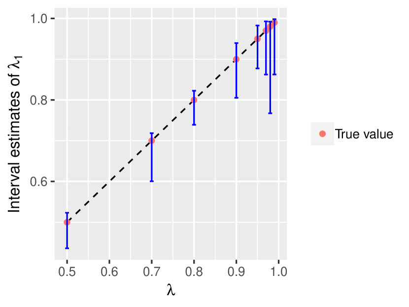
(b) Interval estimates for $\lambda_{1}$.

Figure 1: Spectral gap estimation for the Gaussian chain for different $\lambda$s

We now add an additional parameter to our toy example in order to study the effect of a closing spectral gap on our method. In particular, let $\pi_{V|U}(\cdot|u)$, $u\in\mathbb{R}$, be the pdf of $\mbox{N}(\lambda u,\lambda(1-\lambda)/2)$, where $\lambda\in(0,1)$. Note that our original example corresponds to $\lambda=1/2$. The eigenvalues of the resultant DA operator are $\{\lambda_{i}\}_{i=0}^{\infty}=\{\lambda^{i}\}_{i=0}^{\infty}$. We investigate the effectiveness of our method as $\lambda_{1}=\lambda$ goes to $1$, that is, as the spectral gap $\delta=1-\lambda$ closes. To this end, consider a sequence of Gaussian chains with $\lambda$ increasing from $0.5$ to $0.99$. In accordance with the discussion in Section 6, for a given $\lambda$, we set $\omega$ to be the density function of a $t$-distribution with similar variance as $\pi_{V}(\cdot)$, which is the pdf of $\mbox{N}(0,\lambda/2)$. One can verify that (15) holds for every $\lambda\in(0,1)$. Note that in order for $u_{k}=(s_{k}-1)^{1/k}$ to be a non-trivial upper bound on $\lambda_{1}$, we need $s_{k}<2$. As $\lambda$ increases, so does $s_{k}$ for any given $k$, and thus one must increase $k$ in order to find a useful upper bound. Figure 1(a) shows the $k$s used for different $\lambda$s. When $\lambda=0.5$, we only need $k=4$ to get a decent result; but when $\lambda=0.99$, $k\approx 70$ is needed. Recall that the time needed to run $N$ iterations of Algorithm 1 is approximately $kN\tau$, where $\tau$ is the time needed to simulate one step of the DA chain, which is roughly the same for any $\lambda\in(0,1)$. To compare the performance of our method for different $\lambda$s, we fix $kN=1\times 10^{6}$, and compare the length of the interval estimates of $\lambda_{1}$. The results are shown in Figure 1(b). As $\lambda$ grows, so does $k$, and we are forced to use a smaller sample size $N$. Thus, as $\lambda$ grows, it becomes more difficult to estimate the variances of $u_{k}^{*}$ and $l_{k}^{*}$ accurately. As a result, the length of the interval estimate of $\lambda_{1}$ becomes less stable when $\lambda$ is near $1$. This is reflected in Figure 1(b) by an unusually wide interval estimate at $\lambda=0.97$. On the other hand, most of the interval estimates at other values of $\lambda$ near $1$ are reasonably well-behaved.

7.2 Bayesian probit regression

Let $Y_{1},Y_{2},\dots,Y_{n}$ be independent Bernoulli random variables with $\mathbb{P}(Y_{1}=1|\beta)=\Phi(x_{i}^{T}\beta),$ where $x_{i},\beta\in\mathbb{R}^{p}$, and $\Phi(\cdot)$ is the cumulative distribution function of the standard normal distribution. Take the prior on $\beta$ to be $\mbox{N}_{p}(Q^{-1}w,Q^{-1}),$ where $w\in\mathbb{R}^{p}$ and $Q$ is positive definite. The resulting posterior distribution is intractable, but Albert and Chib (1993) devised a DA algorithm to sample from it. Let $z=(z_{1},z_{2},\dots,z_{n})^{T}$ be a vector of latent variables, and let $X$ be the design matrix whose $i$th row is $x_{i}^{T}.$ The Mtd of the Albert and Chib (AC) chain, $p(\beta,\cdot),\beta\in\mathbb{R}^{p},$ is characterized by

$$\pi_{U|V}(\beta|z)\propto\exp\bigg{[}-\frac{1}{2}\big{\{}\beta-\big{(}X^{T}X+Q\big{)}^{-1}\big{(}w+X^{T}z\big{)}\big{\}}^{T}\big{(}X^{T}X+Q\big{)}\big{\{}\beta-\big{(}X^{T}X+Q\big{)}^{-1}\big{(}w+X^{T}z\big{)}\big{\}}\bigg{]}\,,$$

and

$$\pi_{V|U}(z|\beta)\propto\prod_{i=1}^{n}\exp\bigg{\{}-\frac{1}{2}\big{(}z_{i}-x_{i}^{T}\beta\big{)}^{2}\bigg{\}}I_{\mathbb{R}_{+}}\big{(}(y_{i}-0.5)z_{i}\big{)}\,.$$

The first conditional density, $\pi_{U|V}(\cdot|z)$, is a multivariate normal density, and the second conditional density, $\pi_{V|U}(\cdot|\beta)$, is a product of univariate truncated normal pdfs.

A sandwich step can be added to facilitate the convergence of the AC chain. Chakraborty and Khare (2017) constructed a Haar PX-DA variant of the chain, which is a sandwich chain with transition density of the form (6) (see also Roy and Hobert (2007)). The sandwich step $s(z,dz^{\prime})$ is equivalent to the following update: $z\mapsto z^{\prime}=gz$, where the scalar $g$ is drawn from the following density:

$$\pi_{G}(g|z)\propto g^{n-1}\exp\bigg{[}-\frac{1}{2}z^{T}\big{\{}I_{n}-X(X^{T}X+Q)^{-1}X^{T}\big{\}}zg^{2}+z^{T}X(X^{T}X+Q)^{-1}wg\bigg{]}.$$

Note that this pdf is particularly easy to sample from when $w=0$.

Chakraborty and Khare (2017) showed that, for the AC chain, $P$ is trace-class when one uses a concentrated prior (corresponding to $Q$ having large eigenvalues). In fact, the following is shown to hold in their proof.

Proposition 6.

Suppose that $X$ is full rank. If all the eigenvalues of $Q^{-1/2}X^{T}XQ^{-1/2}$ are less than $7/2,$ then for any polynomial function $t:\mathbb{R}^{p}\to\mathbb{R}$,

$$\int_{\mathbb{R}^{p}}|t(\beta)|p(\beta,\beta)\,d\beta<\infty\,.$$

We will use the estimator (18). The following proposition provides a class of $\psi(\cdot)$s that lead to estimators with finite variance.

Proposition 7.

Suppose the hypothesis in Proposition 6 holds. If $\psi(\cdot)$ is the pdf of a $p$-variate $t$-distribution, i.e.

$$\psi(\beta)\propto\bigg{\{}1+\frac{1}{a}(\beta-b)^{T}\Sigma^{-1}(\beta-b)\bigg{\}}^{-(a+p)/2}$$

for some $b\in\mathbb{R}^{p},$ positive definite matrix $\Sigma\in\mathbb{R}^{p\times p},$ and positive integer $a,$ then the estimator (18) has finite variance.

Proof.

Note that for every $\beta$ and $z$

$$\pi^{3}_{U|V}(\beta|z)\leq C\pi_{U|V}(\beta|z)\,,$$

where $C$ is a constant. Hence, by Proposition 6, for any polynomial function $t:\mathbb{R}^{p}\to\mathbb{R},$

$$\int_{\mathbb{R}^{p}}\int_{\mathbb{R}^{n}}|t(\beta)|\pi^{3}_{U|V}(\beta|z)\pi_{V|U}(z|\beta)\,dz\,d\beta\leq C\int_{\mathbb{R}^{p}}|t(\beta)|p(\beta,\beta)\,d\beta<\infty.$$

Since $\psi^{-2}(\cdot)$ is a polynomial function on $\mathbb{R}^{p}$, the moment condition (20) holds. The result follows from Corollary 5. ∎

As a numerical illustration, we apply our method to the Markov operator associated with the AC chain corresponding to the famous “lupus data” of van Dyk and Meng (2001). In this dataset, $n=55$ and $p=3$. We will construct an asymptotically valid 95% CI for the second largest eigenvalue, and this appears to be the most rigorous and detailed analysis to date of the spectrum of a practically relevant MCMC algorithm on an uncountable state space. As in Chakraborty and Khare (2017), we will let $w=0$ and $Q=X^{T}X/c$, where $c=3.499999$. It can be easily shown that the assumptions in Proposition 6 are met. Chakraborty and Khare (2017) compared the AC chain, $\Phi$, and its Haar PX-DA variant, $\tilde{\Phi}$, defined a few paragraphs ago. This comparison was done using estimated autocorrelations. Their results suggest that $\tilde{\Phi}$ outperforms $\Phi$ when estimating a certain test function. We go further and estimate the second largest eigenvalue of each operator.

It can be shown that the posterior pdf, $\pi_{U}(\cdot)$, is log-concave, and thus possess a unique mode. Let $\hat{\beta}$ be the posterior mode, and $\hat{\Sigma}$ the estimated variance of the MLE. We pick $\psi(\cdot)$ to be the pdf of $t_{30}(\hat{\beta},(\hat{\Sigma}^{-1}+Q)^{-1}).$ This is to say, for any $\beta\in\mathbb{R}^{p},$

$$\psi(\beta)\propto\Big{\{}1+\frac{1}{30}(\beta-\hat{\beta})^{T}(\hat{\Sigma}^{-1}+Q)(\beta-\hat{\beta})\Big{\}}^{-(p+30)/2}.$$

By Proposition 7, this choice of $\psi(\cdot)$ guarantees finite variance. When $n$ is large, $\psi(\cdot)$ is expected to resemble $\pi_{U}(\cdot)$. The performance of our method seems insensitive to the degrees of freedom of the $t$-distribution (which is set at 30 for illustration).

We use a Monte Carlo sample size of $N=4\times 10^{5}$ to form our estimates for the DA operator, and the results are shown in Table 2. Asymptotic $95\%$ CIs for $l_{5}$ and $u_{5}$ are $(0.397,0.545)$ and $(0.573,0.595)$, respectively. Using a Bonferroni argument, we can state that asymptotically, with at least $95\%$ confidence, $\lambda_{1}\in(0.397,0.595)$.

Table 2: Estimated power sums of eigenvalues for the AC chain

$k$	Est. $s_{k}$	Est. $D^{\prime}/\sqrt{N}$	Est. $l_{k}$	Est. $u_{k}$
$1$	$6.744$	$0.072$	$0.000$	$5.744$
$2$	$2.041$	$0.007$	$0.181$	$1.020$
$3$	$1.363$	$0.004$	$0.349$	$0.713$
$4$	$1.156$	$0.004$	$0.430$	$0.628$
$5$	$1.068$	$0.003$	$0.436$	$0.584$

Table 3: Estimated power sums of eigenvalues for the Haar PX-DA version of the AC chain

$k$	Est. $\tilde{s}_{k}$	Est. $D^{\prime}/\sqrt{N}$	Est. $\tilde{l}_{k}$	Est. $\tilde{u}_{k}$
$1$	$3.796$	$0.012$	$0.000$	$1.796$
$2$	$1.538$	$0.004$	$0.193$	$0.734$
$3$	$1.172$	$0.004$	$0.319$	$0.556$
$4$	$1.060$	$0.003$	$0.352$	$0.496$
$5$	$1.025$	$0.003$	$0.419$	$0.479$

We now consider the sandwich chain, $\tilde{\Phi}$. It is known that the Mtd of any Haar PX-DA chain is representable (Hobert and Marchev, 2008). Hence, $\tilde{P}$ is indeed a DA operator. Recall that $\{\tilde{\lambda}_{i}\}_{i=0}^{\tilde{\kappa}},\,0\leq\tilde{\kappa}\leq\infty$, denote the decreasingly ordered positive eigenvalues of $\tilde{P}$. It was shown in Khare and Hobert (2011) that $\tilde{\lambda}_{i}\leq\lambda_{i}$ for $i\in\mathbb{N}$ with at least one strict inequality. For a positive integer $k,$ $\sum_{i=0}^{\tilde{\kappa}}\tilde{\lambda}_{i}^{k}$ is denoted by $\tilde{s}_{k}$. Let $\tilde{u}_{k}$ and $\tilde{l}_{k},$ be the respective counterparts of $u_{k}$ and $l_{k}$. Estimates of $\tilde{s}_{k},\,k=1,2,\cdots,5$ using $4\times 10^{5}$ Monte Carlo samples are given in Table 3. Our estimate of $\tilde{s}_{1}-1$ is less than half of $s_{1}-1$, implying that, in an average sense, the sandwich version of the AC chain reduces the nontrivial eigenvalues of $P$ by more than half. Asymptotic $95\%$ CIs for $\tilde{l}_{5}$ and $\tilde{u}_{5}$ are $(0.321,0.518)$ and $(0.456,0.503)$. Thus, asymptotically, with at least $95\%$ confidence, $\tilde{\lambda}_{1}\in(0.321,0.503)$. The method does not detect a significant difference between $\lambda_{1}$ and $\tilde{\lambda}_{1}$.

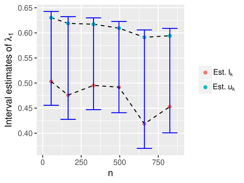
(a) Interval estimates for $\lambda_{1}$ for different $n$s.

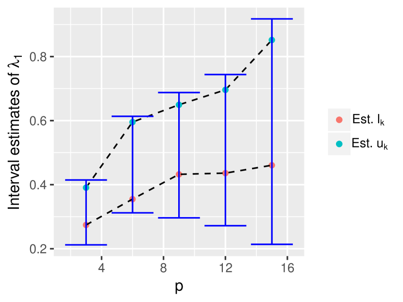
(b) Interval estimates for $\lambda_{1}$ for different $p$s.

Figure 2: Spectral gap estimation for the AC chain

We now study the performance of our method when $n$ or $p$ increases for the original AC chain. First, consider a sequence of datasets where $n$ grows. Let $X_{\scriptsize\mbox{lupus}}\in\mathbb{R}^{55\times 3}$ be the design matrix for the lupus data, and let $r$ be a positive integer. Set $X\in\mathbb{R}^{n\times 3}$ to be $r$ copies of $X_{\scriptsize\mbox{lupus}}$ stacked on top of each other, so that $n=55r$. The response vector $(Y_{1},Y_{2},\dots,Y_{n})^{T}$ is randomly generated in accordance with the probit regression model with the true value of $\beta$ being $(-3,0,3)^{T}$. Let $r$ range from $1$ to $15$. This gives rise to a sequence of datasets with $n$ growing from $55$ to $825$. An interval estimate for $\lambda_{1}$ is then constructed for each of these datasets. Throughout the simulation, $k$ is fixed at $5$, and $N$ is fixed at $4\times 10^{5}$. The result is given in Figure 2(a). Increasing $n$, which is the dimension of $S_{V}$, apparently does not undermine the method.

Now we consider a sequence of datasets where $n$ is fixed and $p$ grows. Let $n=200$, and let $X$ be a $200\times p$ matrix whose $ij$th element is $p_{j}(i)$, with $\{p_{j}(\cdot)\}_{j=1}^{p}$ being a set of orthogonal polynomials generated using the R function poly(). The response vector is randomly generated according to the probit model with the true value of $\beta$ being $(-p,-p+2p/(1-p),-p+4p/(1-p),\cdots,p)^{T}$. We apply our method to such a dataset when $p$ is increased from $3$ to $15$. $N$ is set to be $4\times 10^{5}$, and $k$ is either $4$ or $5$, whichever yields a better estimate. The interval estimates for $\lambda_{1}$ are given in Figure 2(b). As $p$ increases, the length of the interval estimate grows quite rapidly, indicating that the method does not scale well with $p$, that is, the dimension of $S_{U}$. This is consistent with the analysis near the end of Section 5, which suggests that Algorithm 2 works well when $n$ is large and $p$ is small, but not the other way around.

7.3 Bayesian linear regression model with non-Gaussian errors

Let $Y_{1},Y_{2},\dots,Y_{n}$ be independent $d$-dimensional random vectors from the linear regression model

$$Y_{i}=\beta^{T}x_{i}+\Sigma^{1/2}\varepsilon_{i}\,,$$

where $x_{i}\in\mathbb{R}^{p}$ is known, while $\beta\in\mathbb{R}^{p\times d}$ and the $d\times d$ positive definite matrix $\Sigma$ are to be estimated. The iid errors, $\varepsilon_{1},\varepsilon_{2},\dots,\varepsilon_{n}$, are assumed to have a pdf that is a scale mixture of Gaussian densities:

$$f_{h}(\varepsilon)=\int_{\mathbb{R}_{+}}\frac{u^{d/2}}{(2\pi)^{d/2}}\exp\Big{(}-\frac{u}{2}\varepsilon^{T}\varepsilon\Big{)}h(u)\,du,$$

where $h(\cdot)$ is a pdf with positive support, and $\mathbb{R}_{+}:=(0,\infty).$ For instance, if $d=1$ and $h(u)\propto u^{-2}e^{-1/(8u)},$ then $\varepsilon_{1}$ has pdf proportional to $e^{-|\varepsilon|/2}.$

To perform a Bayesian analysis, we require a prior on the unknown parameter, $(\beta,\Sigma)$. We adopt the (improper) Jeffreys prior, given by $1/|\Sigma|^{(d+1)/2}$. Let $y$ represent the $n\times d$ matrix whose $i$th row is the observed value of $Y_{i}$. The following four conditions, which are sufficient for the resulting posterior to be proper (Qin and Hobert, 2018; Fernandez and Steel, 1999), will be assumed to hold:

1. $n\geq p+d$,

2. $(X:y)$ is full rank, where $X$ is the $n\times p$ matrix whose $i$th row is $x_{i}^{T}$,

3. $\int_{\mathbb{R}_{+}}u^{d/2}h(u)\,du<\infty$, and

4. $\int_{\mathbb{R}_{+}}u^{-(n-p-d)/2}h(u)\,du<\infty$.

The posterior density is highly intractable, but there is a well-known DA algorithm to sample from it (Liu, 1996). Under our framework, the DA chain $\Phi$ is characterized by the Mtd

$$p\big{(}(\beta,\Sigma),(\cdot,\cdot)\big{)}=\int_{\mathbb{R}_{+}^{n}}\pi_{U|V}(\cdot,\cdot|z)\pi_{V|U}(z|\beta,\Sigma)\,dz,$$

where $z=(z_{1},z_{2},\dots,z_{n})^{T}$,

$$\pi_{U|V}(\beta,\Sigma|z) \propto|\Sigma|^{-(n+d+1)/2}\prod_{i=1}^{n}\exp\Big{\{}-\frac{z_{i}}{2}\big{(}y_{i}-\beta^{T}x_{i}\big{)}^{T}\Sigma^{-1}\big{(}y_{i}-\beta^{T}x_{i}\big{)}\Big{\}},\,\mbox{and}$$

$$\pi_{V|U}(z|\beta,\Sigma) \propto\prod_{i=1}^{n}z_{i}^{d/2}\exp\Big{\{}-\frac{z_{i}}{2}\big{(}y_{i}-\beta^{T}x_{i}\big{)}^{T}\Sigma^{-1}\big{(}y_{i}-\beta^{T}x_{i}\big{)}\Big{\}}h(z_{i})\,.$$

The first conditional density, $\pi_{U|V}(\cdot,\cdot|z)$, characterizes a multivariate normal distribution on top of an inverse Wishart distribution, i.e. $\beta|\Sigma,z$ is multivariate normal, and $\Sigma|z$ is inverse Wishart. The second conditional density, $\pi_{V|U}(\cdot|\beta,\Sigma)$, is a product of $n$ univariate densities. Moreover, when $h(\cdot)$ is a standard pdf on $\mathbb{R}_{+}$, these univariate densities are often members of a standard parametric family. The following proposition about the resulting DA operator is proved in Qin and Hobert (2018).

Proposition 8.

Suppose $h(\cdot)$ is strictly positive in a neighborhood of the origin. If there exists $\xi\in(1,2)$ and $\delta>0$ such that

$$\int_{0}^{\delta}\frac{u^{d/2}h(u)}{\int_{0}^{\xi u}v^{d/2}h(v)\,dv}\,du<\infty,$$

then $P$ is trace-class.

When $P$ is trace-class, we can pick an $\omega(\cdot)$ and try to make use of (13). A sufficient condition for the estimator’s variance, $D^{2}$, to be finite is stated in the following proposition, whose proof is given in the appendix.

Proposition 9.

Suppose that $h(\cdot)$ is strictly positive in a neighborhood of the origin. If $\omega(z)$ can be written as $\prod_{i=1}^{n}\omega_{i}(z_{i}),$ and there exists $\xi\in(1,4/3)$ such that for all $i\in\{1,2,\dots,n\},$

$$\int_{\mathbb{R}_{+}}\frac{u^{3d/2}h^{3}(u)}{(\int_{0}^{\xi u}v^{d/2}h(v)\,dv)^{3}\omega_{i}^{2}(u)}\,du<\infty,$$ (21)

then (15) holds, and thus by Theorem 4, the estimator (13) has finite variance.

For illustration, take $d=1$ and $h(u)\propto u^{-2}e^{-1/(8u)}$. Then $\varepsilon_{1}$ follows a scaled Laplace distribution, and the model can be viewed as a median regression model with variance $\Sigma$ unknown. It’s easy to show that $h(\cdot)$ satisfies the assumptions in Proposition 8, so the resultant DA operator is trace-class. Now let

$$\omega(z)=\prod_{i=1}^{n}\omega_{i}(z_{i})\propto\prod_{i=1}^{n}z_{i}^{-3/2}e^{-1/(32z_{i})}\,.$$

The following result shows that this will lead to an estimator with finite variance.

Corollary 10.

Suppose $d=1$, $h(u)\propto u^{-2}e^{-1/(8u)}$, and

$$\omega(z)=\prod_{i=1}^{n}\omega_{i}(z_{i})\propto\prod_{i=1}^{n}z_{i}^{-\alpha-1}e^{-\gamma/z_{i}}\,,$$

where $0<\alpha<3/4$ and $0<\gamma<3/64$. Then the variance, $D^{2}$, is finite.

Proof.

In light of Proposition 9, we only need to show that (21) holds for some $\xi\in(1,4/3).$ For any $\xi>0,$ making use of the fact that (by monotone convergence theorem)

$$\lim\limits_{u\to\infty}\int_{0}^{\xi u}v^{1/2}h(v)\,dv=\int_{\mathbb{R}_{+}}u^{1/2}h(u)\,du>0\,,$$

one can easily show for any $\delta>0$,

$$\int_{\delta}^{\infty}\frac{u^{3/2}h^{3}(u)}{(\int_{0}^{\xi u}v^{1/2}h(v)\,dv)^{3}\omega_{i}^{2}(u)}\,du=\int_{\delta}^{\infty}\frac{u^{2\alpha-5/2}\exp\{2\gamma/u-3/(8u)\}}{(\int_{0}^{\xi u}v^{1/2}h(v)\,dv)^{3}}\,du<\infty.$$ (22)

On the other hand, using L’Hôpital’s rule, we can see for $(1-16\gamma/3)^{-1}<\xi<4/3,$

$$\lim\limits_{u\to 0}\Bigg{(}\frac{u^{3/2}h^{3}(u)}{(\int_{0}^{\xi u}v^{1/2}h(v)\,dv)^{3}\omega_{i}^{2}(u)}\Bigg{)}^{1/3} =\lim\limits_{u\to 0}\frac{u^{2\alpha/3-5/6}\exp\{2\gamma/(3u)-1/(8u)\}}{\int_{0}^{\xi u}v^{-3/2}e^{-1/(8v)}\,dv}$$

$$=\lim\limits_{u\to 0}R(u)\exp\Big{\{}-\Big{(}-\frac{2\gamma}{3}-\frac{1}{8\xi}+\frac{1}{8}\Big{)}\frac{1}{u}\Big{\}}$$

$$=0,$$

where $R(u)$ is a function that is either bounded near the origin or goes to $\infty$ at the rate of some power function as $u\to 0.$ It follows that for $\xi\in((1-16\gamma/3)^{-1},4/3)$ and small enough $\delta,$

$$\int_{0}^{\delta}\frac{u^{3/2}h^{3}(u)}{(\int_{0}^{\xi u}v^{1/2}h(v)\,dv)^{3}\omega_{i}^{2}(u)}\,du<\infty.$$ (23)

Combining (22) and (23) yields (21). The result then follows. ∎

(a) Interval estimates for $\lambda_{1}$ for different $n$s.

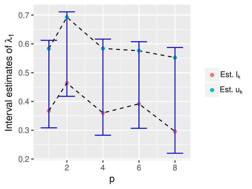
(b) Interval estimates for $\lambda_{1}$ for different $p$s.

Figure 3: Spectral gap estimation for the DA chain for Bayesian linear model

We now test the effectiveness of the Monte Carlo estimator (13) on a sequence of growing datasets with $d=1$. Let $p=3$, and let $X$ be an $n\times p$ design matrix with 3 distinct rows, $(1,0,0)^{T}$, $(0,1,0)^{T}$, and $(0,0,1)^{T}$, each replicated $r$ times, so that $n=3r$. The responses, $Y_{1},Y_{2},\cdots,Y_{n}$, are then generated according to the previously defined linear regression model with the true value of $\beta$ being $(-3,0,3)^{T}$, and the true value of $\Sigma$ being $1$. In other words, $Y_{i}-x_{i}^{T}(-3,0,3)^{T}\sim f_{h}(\cdot)$ independently for each $i$, where $f_{h}(u)\propto e^{-|u|/2}$. The resultant DA chain $\Phi$ lives in $S_{U}=\mathbb{R}^{3}\times\mathbb{R}_{+}$, and $S_{V}=\mathbb{R}^{n}=\mathbb{R}^{3r}$. Let $r$ grow from $2$ to $6$. We use a Monte Carlo sample size of $N=2\times 10^{6}$ to form interval estimates of $\lambda_{1}$ for different values of $r$. For simplicity, we fix $k$ to be $4$. The results are given in Figure 3(a). As $n$ grows, the length of the interval estimate increases quite rapidly. This is understandable, since our method is essentially an importance sampling technique, which does not work well in high dimensional settings unless tuned with great care. In the previous subsection where we study Bayesian probit regression, we are able to easily deal with a dataset with $n>800$. Part of the reason is that, in that case, Algorithm 2 is used, and since $S_{U}$ is low dimensional, it’s easy to choose $\psi(\cdot)$ that resembles $\pi_{U}(\cdot)$.

Consider another sequence of datasets where $d=1$, $n=10$, and $p$ is increased from $1$ to $8$. The $ij$th element of the design matrix $X$ is set to be $p_{j}(i)$, where $\{p_{j}(\cdot)\}_{j=1}^{p}$ are orthogonal polynomials generated in R. The responses are generated according to the aforementioned linear regression model with the true value of $\beta$ being $(-p,p+2p/(1-p),-p+4p/(1-p),\dots,p)^{T}$, and the true value of $\Sigma$ being $1$. In this case, $S_{U}=\mathbb{R}^{p}\times\mathbb{R}_{+}$, and $S_{V}=\mathbb{R}^{10}$. Using a Monte Carlo sample size of $N=2\times 10^{6}$ and setting $k=4$, we obtain interval estimates of $\lambda_{1}$ for different $p$s. The results are given in Figure 3(b). Compare this to the case where $p$ is fixed an $n$ grows. We see that the effectiveness of Algorithm 1, characterized by the length of the interval estimate it produces, is much less susceptible to the growing dimension of $S_{U}$ than to that of $S_{V}$.

Acknowledgment. The second and third authors were supported by NSF Grant DMS-15-11945.

Appendix

Appendix A Proof of Theorem 2

Theorem 2.  The DA operator $P$ is trace-class if and only if

$$\int_{S_{U}}p(u,u)\,\mu(du)<\infty.$$ (4)

If (4) holds, then for any positive integer $k,$

$$s_{k}:=\sum_{i=0}^{\kappa}\lambda_{i}^{k}=\int_{S_{U}}p^{(k)}(u,u)\,\mu(du)<\infty.$$ (5)

Proof.

Note that $P$ is self-adjoint and non-negative. Let $\{g_{i}\}_{i=0}^{\infty}$ be an orthonormal basis of $L^{2}(\pi_{U})$. The operator $P$ is defined to be trace-class if (see e.g. Conway, 2000)

$$\sum_{i=0}^{\infty}\langle Pg_{i},g_{i}\rangle_{\pi_{U}}<\infty.$$ (24)

This condition is equivalent to $P$ being compact with summable eigenvalues. To show that $P$ being trace-class is equivalent to (4), we will prove a stronger result, namely

$$\sum_{i=0}^{\infty}\langle Pg_{i},g_{i}\rangle_{\pi_{U}}=\int_{S_{U}}p(u,u)\mu(du).$$ (25)

We begin by defining two new Hilbert spaces. Let $L^{2}(\pi_{V})$ be the Hilbert space consisting of functions that are square integrable with respect to the weight function $\pi_{V}(\cdot).$ For $f,g\in L^{2}(\pi_{V}),$ their inner product is defined, as usual, by

$$\langle f,g\rangle_{\pi_{V}}=\int_{S_{V}}f(v)\overline{g(v)}\pi_{V}(v)\,\nu(dv).$$

Let $L^{2}(\pi_{U}\times\pi_{V})$ be the Hilbert space of functions on $S_{U}\times S_{V}$ that are square integrable with respect to the weight function $\pi_{U}(\cdot)\pi_{V}(\cdot).$ For $f,g\in L^{2}(\pi_{U}\times\pi_{V}),$ their inner product is

$$\langle f,g\rangle_{\pi_{U}\times\pi_{V}}=\int_{S_{U}\times S_{V}}f(u,v)\overline{g(u,v)}\pi_{U}(u)\pi_{V}(v)\,\mu(du)\,\nu(dv).$$

Note that $L^{2}(\pi_{V})$ is separable. Let $\{h_{j}\}_{j=0}^{\infty}$ be an orthonormal basis of $L^{2}(\pi_{V}).$ It can be shown that $\{g_{i}h_{j}\}_{(i,j)\in\mathbb{Z}_{+}^{2}}$ is an orthonormal basis of $L^{2}(\pi_{U}\times\pi_{V})$. Of course, $g_{i}h_{j}$ denotes the function given by $(g_{i}h_{j})(u,v)=g_{i}(u)h_{j}(v).$

The inequality (4) is equivalent to

$$\int_{S_{U}\times S_{V}}\bigg{(}\frac{\pi_{U,V}(u,v)}{\pi_{U}(u)\pi_{V}(v)}\bigg{)}^{2}\pi_{U}(u)\pi_{V}(v)\,\mu(du)\,\nu(dv)<\infty,$$

which holds if and only if the function $\varphi:S_{U}\times S_{V}\to\mathbb{R}$ given by

$$\varphi(u,v)=\frac{\pi_{U,V}(u,v)}{\pi_{U}(u)\pi_{V}(v)}$$

is in $L^{2}(\pi_{U}\times\pi_{V}).$ Suppose (4) holds. Then by Parseval’s identity,

$$\int_{S_{U}}p(u,u)\,\mu(du) =\langle\varphi,\varphi\rangle_{\pi_{U}\times\pi_{V}}$$

$$=\sum_{(i,j)\in\mathbb{Z}_{+}^{2}}|\langle\varphi,g_{i}h_{j}\rangle_{\pi_{U}\times\pi_{V}}|^{2}$$

$$=\sum_{(i,j)\in\mathbb{Z}_{+}^{2}}\Big{|}\int_{S_{U}\times S_{V}}\overline{g_{i}(u)}\overline{h_{j}(v)}\pi_{U,V}(u,v)\,\mu(du)\,\nu(dv)\Big{|}^{2}$$

$$=\sum_{i=0}^{\infty}\sum_{j=0}^{\infty}\Big{|}\int_{S_{V}}\Big{(}\int_{S_{U}}\overline{g_{i}(u)}\pi_{U|V}(u|v)\,\mu(du)\Big{)}\overline{h_{j}(v)}\pi_{V}(v)\,\nu(dv)\Big{|}^{2}.$$

Again by Parseval’s identity, this time applied to the function on $S_{V}$ (and in fact, in $L^{2}(\pi_{V})$ by Jensen’s inequality) given by

$$\varphi_{i}(v)=\int_{S_{U}}\overline{g_{i}(u)}\pi_{U|V}(u|v)\,\mu(du),$$

we have

$$\int_{S_{U}}p(u,u)\,\mu(du) =\sum_{i=0}^{\infty}\sum_{j=0}^{\infty}|\langle\varphi_{i},h_{j}\rangle_{\pi_{V}}|^{2}$$ (26)

$$=\sum_{i=0}^{\infty}\langle\varphi_{i},\varphi_{i}\rangle_{\pi_{V}}$$

$$=\sum_{i=0}^{\infty}\int_{S_{V}}\Big{|}\int_{S_{U}}\overline{g_{i}(u)}\pi_{U|V}(u|v)\,\mu(du)\Big{|}^{2}\pi_{V}(v)\,\nu(dv)$$

$$=\sum_{i=0}^{\infty}\int_{S_{V}}\int_{S_{U}}\Big{(}\int_{S_{U}}g_{i}(u^{\prime})\pi_{U|V}(u^{\prime}|v)\pi_{V|U}(v|u)\,\mu(du^{\prime})\Big{)}\overline{g_{i}(u)}\pi_{U}(u)\,\mu(du)\,\nu(dv)$$

$$=\sum_{i=0}^{\infty}\int_{S_{U}}\Big{(}\int_{S_{U}}p(u,u^{\prime})g_{i}(u^{\prime})\,\mu(du^{\prime})\Big{)}\overline{g_{i}(u)}\pi_{U}(u)\,\mu(du).$$

Note that the use of Fubini’s theorem in the last equality can be easily justified by noting that $g_{i}\in L^{2}(\pi_{U})$, and making use of Jensen’s inequality. But the right hand side of (26) is precisely $\sum_{i=0}^{\infty}\langle Pg_{i},g_{i}\rangle_{\pi_{U}}.$ Hence, (25) holds when $\int_{S_{U}}p(u,u)\,\mu(du)$ is finite.

To finish our proof of (25), we’ll show (24) implies (4). Assume that (24) holds. Tracing backwards along (26) yields

$$\sum_{(i,j)\in\mathbb{Z}_{+}^{2}}|\langle\varphi_{i},h_{j}\rangle_{\pi_{V}}|^{2}<\infty.$$

This implies that the function

$$\tilde{\varphi}:=\sum_{(i,j)\in\mathbb{Z}_{+}^{2}}\langle\varphi_{i},h_{j}\rangle_{\pi_{V}}g_{i}h_{j}$$

is in $L^{2}(\pi_{U}\times\pi_{V}).$ Recall that (4) is equivalent to $\varphi$ being in $L^{2}(\pi_{U}\times\pi_{V}).$ Hence, it suffices to show that $\tilde{\varphi}(u,v)=\varphi(u,v)$ almost everywhere. Define a linear transformation $T:L^{2}(\pi_{U})\to L^{2}(\pi_{V})$ by

$$Tf(v)=\int_{S_{U}}f(u)\pi_{U|V}(u|v)\,\mu(du),\quad\forall f\in L^{2}(\pi_{U}).$$

By Jensen’s inequality, $T$ is bounded, and thus, continuous. For any $g=\sum_{i=0}^{\infty}\alpha_{i}g_{i}\in L^{2}(\pi_{U})$ and $h=\sum_{j=0}^{\infty}\beta_{j}h_{j}\in L^{2}(\pi_{V}),$

$$\int_{S_{V}}\int_{S_{U}}\varphi(u,v)\overline{g(u)}\overline{h(v)}\,\pi_{U}(u)\pi_{V}(v)\,\mu(du)\,\nu(dv)$$

$$=\langle T\overline{g},h\rangle_{\pi_{V}}$$

$$=\sum_{i=0}^{\infty}\sum_{j=0}^{\infty}\overline{\alpha_{i}\beta_{j}}\langle T\overline{g_{i}},h_{j}\rangle_{\pi_{V}}$$

$$=\sum_{i=0}^{\infty}\sum_{j=0}^{\infty}\overline{\alpha_{i}\beta_{j}}\langle\varphi_{i},h_{j}\rangle_{\pi_{V}}$$

$$=\langle\tilde{\varphi},gh\rangle_{\pi_{U}\times\pi_{V}}$$

$$=\int_{S_{V}}\int_{S_{U}}\tilde{\varphi}(u,v)\overline{g(u)}\overline{h(v)}\,\pi_{U}(u)\pi_{V}(v)\,\mu(du)\,\nu(dv),$$

where $\overline{g}\in L^{2}(\pi_{V})$ is given by $\overline{g}(u):=\overline{g(u)},$ and $\overline{g_{i}}$ is defined similarly for $i\in\mathbb{Z}_{+}$. This implies that for any $C_{1}\in\mathcal{U}$ and $C_{2}\in\mathcal{V},$

$$\int_{C_{1}\times C_{2}}\varphi(u,v)\,\pi_{U}(u)\pi_{V}(v)\,\mu(du)\,\nu(dv)=\int_{C_{1}\times C_{2}}\tilde{\varphi}(u,v)\,\pi_{U}(u)\pi_{V}(v)\,\mu(du)\,\nu(dv).$$

Note that

$$\int_{S_{U}\times S_{V}}|\tilde{\varphi}(u,v)|\,\pi_{U}(u)\pi_{V}(v)\,\mu(du)\,\nu(dv)\leq\langle\tilde{\varphi},\tilde{\varphi}\rangle_{\pi_{U}\times\pi_{V}}^{1/2}<\infty.$$ (27)

By (27) and the dominated convergence theorem, one can show that

$$\mathcal{A}:=\Big{\{}C\in\mathcal{U}\times\mathcal{V}\,\Big{|}\,\int_{C}\varphi(u,v)\,\pi_{U}(u)\pi_{V}(v)\,\mu(du)\,\nu(dv)=\int_{C}\tilde{\varphi}(u,v)\,\pi_{U}(u)\pi_{V}(v)\,\mu(du)\,\nu(dv)\Big{\}}$$

is a $\lambda$ system. An application of Dynkin’s $\pi$-$\lambda$ theorem reveals that $\mathcal{\mathcal{U}\times\mathcal{V}}\subset\mathcal{A}.$ Therefore, $\tilde{\varphi}(u,v)=\varphi(u,v)$ almost everywhere, and (4) follows.

For the rest of the proof, assume that $P$ is trace-class. This implies that $P$ is compact, and thus admits the spectral decomposition (see e.g. Helmberg, 2014, §28 Corollary 2.1) given by

$$Pf=\sum_{i=0}^{\kappa}\lambda_{i}\langle f,f_{i}\rangle_{\pi_{U}}f_{i},\quad f\in L^{2}(\pi_{U})$$ (28)

where $f_{i},\,i=0,1,\dots,\kappa,$ is the normalized eigenfunction corresponding to $\lambda_{i}.$ By Parseval’s identity,

$$\sum_{i=0}^{\infty}\langle Pg_{i},g_{i}\rangle_{\pi_{U}} =\sum_{i=0}^{\infty}\sum_{j=0}^{\kappa}\lambda_{j}|\langle g_{i},f_{j}\rangle_{\pi_{U}}|^{2}$$

$$=\sum_{j=0}^{\kappa}\lambda_{j}\langle f_{j},f_{j}\rangle_{\pi_{U}}$$

$$=\sum_{j=0}^{\kappa}\lambda_{j}.$$

This equality is in fact a trivial case of Lidskii’s theorem (see e.g. Erdös, 1974; Gohberg et al., 2012). It follows that (5) holds for $k=1.$

We now consider the case where $k\geq 2.$ By (28) and a simple induction, we have the following decomposition for $P^{k}.$

$$P^{k}f=\sum_{i=0}^{\kappa}\lambda_{i}^{k}\langle f,f_{i}\rangle_{\pi_{U}}f_{i},\quad f\in L^{2}(\pi_{U})\,.$$

Hence $P^{k}$ is trace-class with ordered positive eigenvalues $\{\lambda_{i}^{k}\}_{i=0}^{\kappa}.$ Note that $P^{k}$ is a Markov operator whose Mtd is $p^{(k)}(u,\cdot),\,u\in S_{U}.$ Thus, in order to show that (5) holds for $k\geq 2,$ it suffices to verify $P^{k}$ is a DA operator, for then we can treat $P^{k}$ as $P$ and repeat our argument for the $k=1$ case. To be specific, we’ll show that there exists a random variable $\tilde{V}$ taking values on $S_{\tilde{V}},$ where $(S_{\tilde{V}},\mathcal{\tilde{V}},\tilde{\nu})$ is a $\sigma$-finite measure space and $\mathcal{\tilde{V}}$ is countably generated, such that for $u\in S_{U},$

$$p^{(k)}(u,\cdot)=\int_{S_{\tilde{V}}}\pi_{U|\tilde{V}}(\cdot|v)\pi_{\tilde{V}|U}(v|u)\,\tilde{\nu}(dv),$$ (29)

where $\pi_{\tilde{V}}(\cdot),$ $\pi_{U|\tilde{V}}(\cdot|\cdot),$ and $\pi_{\tilde{V}|U}(\cdot|\cdot)$ have the apparent meanings.

Let $(U_{k},V_{k})_{k=0}^{\infty}$ be a Markov chain. Suppose that $U_{0}$ has pdf $\pi_{U}(\cdot)$, and for any non-negative integer $k,$ let $V_{k}|U_{k}=u$ have pdf $\pi_{V|U}(\cdot|u),$ and let $U_{k+1}|V_{k}=v$ have pdf $\pi_{U|V}(\cdot|v).$ It’s easy to see $\{U_{k}\}_{k=0}^{\infty}$ is a stationary DA chain with Mtd $p(u,\cdot).$ Suppose $k$ is even. The pdf of $U_{k}|U_{0}=u$ is

$$p^{(k)}(u,\cdot)=\int_{S_{U}}p^{(k/2)}(u,u^{\prime})p^{(k/2)}(u^{\prime},\cdot)\mu(du).$$

Meanwhile, since the chain is reversible and starts from the stationary distribution, $U_{0}|U_{k/2}=u$ has the same distribution as $U_{k/2}|U_{0}=u,$ which is just $p^{(k/2)}(u,\cdot).$ Thus, (29) holds with $\tilde{V}=U_{k/2}.$ A similar argument shows that when $k$ is odd, (29) holds with $\tilde{V}=V_{(k-1)/2}.$ ∎

Appendix B Proof of Proposition 9

Proposition 9.  Suppose that $h(\cdot)$ is strictly positive in a neighborhood of the origin. If $\omega(z)$ can be written as $\prod_{i=1}^{n}\omega_{i}(z_{i}),$ and there exists $\xi\in(1,4/3)$ such that for all $i\in\{1,2,\dots,n\},$

$$\int_{\mathbb{R}_{+}}\frac{u^{3d/2}h^{3}(u)}{(\int_{0}^{\xi u}v^{d/2}h(v)\,dv)^{3}\omega_{i}^{2}(u)}\,du<\infty,$$

then (15) holds, and thus by Theorem 4, second moment exists for the estimator (13).

Proof.

Let $S_{d}$ be the set of $d\times d$ positive definite matrices. For any $\beta\in\mathbb{R}^{p},$ $\Sigma\in S_{d},$ $z\in\mathbb{R}^{n},$ and $\xi\in(1,4/3),$

$$\pi_{U|V}(\beta,\Sigma|z)\pi^{3}_{V|U}(z|\beta,\Sigma)$$

$$=\frac{|\Sigma|^{-(n+d+1)/2}\prod_{i=1}^{n}\exp\{-z_{i}(y_{i}-\beta^{T}x_{i})^{T}\Sigma^{-1}(y_{i}-\beta^{T}x_{i})/2\}}{\int_{\mathbb{R}^{p}}\int_{S_{d}}|\tilde{\Sigma}|^{-(n+d+1)/2}\prod_{i=1}^{n}\exp\{-z_{i}(y_{i}-\tilde{\beta}^{T}x_{i})^{T}\tilde{\Sigma}^{-1}(y_{i}-\tilde{\beta}^{T}x_{i})/2\}\,d\tilde{\Sigma}\,d\tilde{\beta}}\times$$

$$\quad\quad\prod_{i=1}^{n}\frac{z_{i}^{3d/2}\exp\{-3z_{i}(y_{i}-\beta^{T}x_{i})^{T}\Sigma^{-1}(y_{i}-\beta^{T}x_{i})/2\}h^{3}(z_{i})}{\{\int_{0}^{\infty}v^{d/2}\exp[-v(y_{i}-\beta^{T}x_{i})^{T}\Sigma^{-1}(y_{i}-\beta^{T}x_{i})/2]h(v)\,dv\}^{3}}$$

$$\leq\frac{|\Sigma|^{-(n+d+1)/2}\prod_{i=1}^{n}\exp\{-z_{i}(y_{i}-\beta^{T}x_{i})^{T}[\Sigma/(4-3\xi)]^{-1}(y_{i}-\beta^{T}x_{i})/2\}}{\int_{\mathbb{R}^{p}}\int_{S_{d}}|\tilde{\Sigma}|^{-(n+d+1)/2}\prod_{i=1}^{n}\exp\{-z_{i}(y_{i}-\tilde{\beta}^{T}x_{i})^{T}\tilde{\Sigma}^{-1}(y_{i}-\tilde{\beta}^{T}x_{i})/2\}\,d\tilde{\Sigma}\,d\tilde{\beta}}\times$$

$$\quad\quad\prod_{i=1}^{n}\frac{z_{i}^{3d/2}h^{3}(z_{i})}{(\int_{0}^{\xi z_{i}}v^{d/2}h(v)\,dv)^{3}}.$$

Note that

$$\int_{S_{d}}|\Sigma|^{-(n+d+1)/2}\prod_{i=1}^{n}\exp\bigg{\{}-\frac{z_{i}}{2}\big{(}y_{i}-\beta^{T}x_{i}\big{)}^{T}\bigg{(}\frac{\Sigma}{4-3\xi}\bigg{)}^{-1}\big{(}y_{i}-\beta^{T}x_{i}\big{)}\bigg{\}}\,d\Sigma$$

$$=(4-3\xi)^{-nd/2}\int_{S_{d}}|\Sigma|^{-(n+d+1)/2}\prod_{i=1}^{n}\exp\Big{\{}-\frac{z_{i}}{2}\big{(}y_{i}-\beta^{T}x_{i}\big{)}^{T}\Sigma^{-1}\big{(}y_{i}-\beta^{T}x_{i}\big{)}\Big{\}}\,d\Sigma.$$

Thus,

$$\int_{\mathbb{R}^{p}}\int_{S_{d}}\pi_{U|V}(\beta,\Sigma|z)\pi^{3}_{V|U}(z|\beta,\Sigma)\,d\Sigma\,d\beta\leq(4-3\xi)^{-nd/2}\prod_{i=1}^{n}\frac{z_{i}^{3d/2}h^{3}(z_{i})}{(\int_{0}^{\xi z_{i}}v^{d/2}h(v)\,dv)^{3}}.$$

The result follows immediately. ∎

References

- Ahues et al. (2001) Ahues, M., Largillier, A. and Limaye, B. (2001). Spectral Computations for Bounded Operators. CRC Press.
- Albert and Chib (1993) Albert, J. H. and Chib, S. (1993). Bayesian analysis of binary and polychotomous response data. Journal of the American statistical Association 88 669–679.
- Billingsley (1995) Billingsley, P. (1995). Probability and Measure. 3rd ed. John Wiley & Sons.
- Brislawn (1988) Brislawn, C. (1988). Kernels of trace class operators. Proceedings of the American Mathematical Society 104 1181–1190.