Anisotropic magnetoresistance and piezoelectric effect in GaAs Hall samples

Abstract

Application of a strong magnetic field perpendicular to a two-dimensional electron system leads to a variety of quantum phases ranging from incompressible quantum Hall liquid to Wigner solid, charge density wave and exotic non-Abelian states. A few quantum phases seen on past experiments on GaAs Hall samples of electrons show pronounced anisotropic magneto-resistance values at certain weak magnetic fields. We argue that this might be due to the piezoelectric effect that is inherent in a semiconductor host like GaAs. Such an effect has the potential to create a sufficient in-plane internal strain that will be felt by electrons and will determine the direction of high and low resistance. When Wigner solid, charge density wave and isotropic liquid phases are very close in energy, the overall stability of the system is very sensitive to local order and, thus, can be strongly influenced even by a weak perturbation such as the piezoelectric-induced effective electron-electron interaction which is anisotropic. In this work, we argue that an anisotropic interaction potential may stabilize anisotropic liquid phases of electrons even in a strong magnetic field regime where normally one expects to see only isotropic quantum Hall or isotropic Fermi liquid states. We use this approach to support a theoretical framework that envisions the possibility of an anisotropic liquid crystalline state of electrons in the lowest Landau level. In particular, we argue that an anisotropic liquid state of electrons may stabilize in the lowest Landau level close to the liquid-solid transition region at filling factor $\nu=1/6$ for a given anisotropic Coulomb interaction potential. Quantum Monte Carlo simulations for a liquid crystalline state with broken rotational symmetry indicate stability of liquid crystalline order consistent with the existence of an anisotropic liquid state of electrons stabilized by anisotropy at filling factor $\nu=1/6$ of the lowest Landau level.

I Introduction

The study of properties of a strongly correlated two-dimensional electron system (2DES) has always been a fundamental goal of modern condensed matter physics. When a high mobility 2DES typically created in a host GaAs semiconductor environment is placed in a strong perpendicular magnetic field, purely quantum behavior dominates at very low temperatures. The combination of 2D confinement and magnetic field leads to a set of discrete, massively degenerate energy levels well separated from each other known as Landau levels (LLs) labeled by an integer quantum number, $n=0,1,\ldots$. For simplicity of treatment one routinely assumes that the system of electrons is fully spin-polarized. A key parameter that characterizes the properties of a 2DES in a perpendicular magnetic field is the filling factor, $\nu=N/N_{s}$ defined as the ratio of the number of electrons, $N$ to the degeneracy (number of available states), $N_{s}$ of each LL. For an integer number of completely filled LLs, we imagine that the electrons act independently and do not interact with each other jmp-iqhe-one . At very high magnetic fields, when electrons occupy only the lowest Landau level (LLL), correlation effects give rise to fractional quantum Hall effect (FQHE), a novel quantum many-body electronic liquid state tsui82 . The phase diagram of a 2DES in a strong perpendicular magnetic field at filling factors $0<\nu\leq 1$ is intricate with competing liquid and Wigner solid phases. At filling factors, $\nu=1/3,2/5,3/7,\ldots$ and $\nu=1/5,2/9,\ldots$ electrons condense into an incompressible liquid FQHE state. It is believed that at even-denominator filling factors, $\nu=1/2,1/4$ and $1/6$ the electrons form a compressible Fermi liquid state willett1 ; willett2 while for filling factors, $0<\nu\leq 1/7$, Wigner crystallization occurs lam ; esfarjani ; zhu2 . The principal FQHE states at filling factor $\nu=1/3$ and $1/5$ are thoroughly explained and are well described by the Laughlin wave function approach laughlin83 . Other FQHE states at filling factors, $\nu=p/(2mp+1)$ (where $p$ and $m$ are integers) are readily understood in terms of the composite fermion (CF) theory jain ; physe . The $p\rightarrow\infty$ limit of such FQHE states orepjb corresponds to even-denominator filled fractions, $\nu=1/(2m)$ that are believed to be compressible Fermi liquid states qualitatively different from the FQHE states of the originating sequence hlr ; rr ; fantoni4 . While the nature of various quantum states in the LLL seems to be well understood, the situation is more complicated in higher LLs. Fascinating cases are the anisotropic quantum Hall phases lilly at filling factors $\nu=9/2,11/2,\ldots$ in high LLs (where upper LLs with quantum numbers, $n\geq 2$ are partially filled). The observed magneto-resistance anisotropy in such systems has been interpreted as strong evidence for the existence of a unidirectional (or striped) charge-density wave (CDW) state fogler ; moessner . A related possibility consistent with the experimental evidence would view the emergence of anisotropy in this regime as signature of a phase transition from an isotropic to an anisotropic electronic liquid crystalline phase fradkin . This way, one can view the onset of anisotropy as a transition to a quantum Hall nematic state described either as a Pomeranchuk-distorted phase vadim ; doan or as a broken rotational symmetry (BRS) liquid crystalline phase brshalf ; ijmpb ; orion2010 ; cite2011d . In all scenarios above, one assumes a Coulomb interaction between electrons.

II Microscopic Origin of Anisotropy

The microscopic origin of the weak native rotational symmetry breaking potential that may cause preferable orientation of electronic phases relative to the crystallographic axes of the host GaAs material in a GaAs/AlGaAs hetero-structure, so far, has been unclear cooper . Studies in a tilted magnetic field jungwirth ; stanescu indicate that the strength of this anisotropic perturbation is only about $10^{-4}\,e^{2}/l_{0}\approx 1\,mK$ per electron ($l_{0}$ is the electron’s magnetic length). It is also expected that such an anisotropic interaction should be comparatively weak, because the effect of realignment of anisotropy in a tilted magnetic field has been observed lilly2 . One possibility is that the GaAs crystalline substrate itself (coupled to electrons by exchange of phonons) induces a weak angular-dependent correction of the electron-electron Coulomb interaction pan . Emergence of a weak electron-phonon coupling (important below a certain low critical temperature) appears possible.

Based on these considerations, it is reasonable to argue that the precise mechanism which breaks the in-plane symmetry of the 2DES originates from the GaAs host lattice and may be related to the crystal structure of GaAs as well as the particular way of how electrons couple to the lattice in a given GaAs/AlGaAs hetero-structure. We note that GaAs has a zinc-blende cubic structure which is described by two interpenetrating face-centered cubic (fcc) lattices. An important aspect of GaAs crystals is the absence of a center of inversion/symmetry. Hence, GaAs is capable of exhibiting piezoelectric and related effects depending on polar symmetry. Usually the piezoelectric interaction in semiconductors is not of major importance. However, in high quality crystals (such as GaAs Hall samples) and in very low temperatures, this interaction, while weak, can play a role. Given that GaAs is a piezoelectric crystal, we remark that it is possible that the piezoelectric interaction, which is anisotropic for cubic crystals, plays a role in the anisotropic orientation of the given electronic structure hosted there. Clearly, it is possible that the piezoelectric effect inherent in GaAs semiconductor samples can create a sufficient in-plane internal strain which determines the direction of high and low resistance in GaAs Hall samples and, thus, may induce some native anisotropy in the hosted system of electrons.

At this juncture, the key point made is that an anisotropic perturbation term (in general) may explain some basic physics features that control the eventual emergence of anisotropic liquid states of electrons in the quantum Hall regime. As such, this anisotropic term might play an important role in the stability of various electronic phases in all LL-s, including the LLL. In particular, when Wigner solid, CDW and isotropic liquid phases are very close in energy, the overall stability of the system is very sensitive to local order and, thus, can be strongly influenced even by an anisotropic perturbation like the piezoelectric-induced one. This argument leads one to believe that anisotropic phases of electrons may arise even in the strong magnetic field regime (in the LLL) at settings where one would normally expect isotropic fractional quantum Hall liquid, isotropic Fermi liquid, or Wigner solid states. This mechanism may be appealed to explain recent experiments that indicate the presence of a new anisotropic fractional quantum Hall effect state of electrons at regimes not anticipated before abstract3 .

III Anisotropic phases in the lowest Landau level

In earlier work brsall ; hexatic , we investigated the possible existence of anisotropic liquid phases of electrons in the LLL at Laughlin fractions, $\nu=1/3$, $1/5$ and $1/7$. We introduced many-body trial wave functions that are translationally invariant but possess twofold, fourfold, or sixfold BRS at respective filling factors, $\nu=1/3$, $1/5$, and $1/7$ of either the LLL, or excited LLs. We considered a standard Coulomb interaction potential between electrons as well as two other model potentials that include thickness effects. All the electron-electron interaction potentials considered in such a study were isotropic brsall . One of the specific findings was that all the anisotropic liquid crystalline phases considered had higher energy than the competing isotropic Laughlin liquid states in the LLL for systems electrons interacting with the usual isotropic Coulomb potential. Based on these findings we concluded that, if there are electronic liquid states in the LLL, these states are isotropic and should possess rotation symmetry.

However, presence of an anisotropic interaction term in the Hamiltonian reopens the problem and suggests a re-examination of the possibility of anisotropic liquid phases of electrons at all filling factors in the LLL where isotropic liquid states were previously known to exist. We have identified the very fragile isotropic Fermi liquid state kun-yang at $\nu=1/6$ (just before the onset of Wigner crystallization) as a good candidate that may be destabilized by an electron-electron anisotropic perturbation. With this idea in mind, we looked at $\nu=1/6$ and first compared the stability conditions of various known phases such as Wigner solids, Fermi liquids, Bose Laughlin liquids (Wigner crystallization occurs around $\nu=1/6.5$). We found out that different quantum states, for instance, a CF Fermi liquid and a Bose Laughlin state bose have energies extremely close to each other with differences in the order of $10^{-4}\,e^{2}/l_{0}$. Hence, an anisotropic perturbation of comparable magnitude (that can readily be induced) may suffice to shift the energy balance in favour of an anisotropic liquid phase.

Table 1: Roman-numbered energy shells (in $\vec{k}$-space) in increasing order of energy where $g$ is the degeneracy of each energy value, $N$ is the total number of electrons (for a spin-polarized system) and $(n_{x},n_{y})$ are the corresponding plane wave quantum numbers.

Shell	$n_{x}^{2}+n_{y}^{2}$	$g$	$N$	$(n_{x},n_{y})$
I	0	1	1	$(0,0)$
II	1	4	5	$(-1,0),(0,-1),(0,1),(1,0)$
III	2	4	9	$(-1,-1),(-1,1),(1,-1),(1,1)$
IV	4	4	13	$(-2,0),(0,-2),(0,2),(2,0)$
V	5	8	21	$(-2,-1),(-2,1),(-1,-2),(-1,2),(1,-2),(1,2),(2,-1),(2,1)$
VI	8	4	25	$(-2,-2),(-2,2),(2,-2),(2,2)$
VII	9	4	29	$(-3,0),(0,-3),(0,3),(3,0)$
VIII	10	8	37	$(-3,-1),(-3,1),(-1,-3),(-1,3),(1,-3),(1,3),(3,-1),(3,1)$
IX	13	8	45	$(-3,-2),(-3,2),(-2,-3),(-2,3),(2,-3),(2,3),(3,-2),(3,2)$
X	16	4	49	$(-4,0),(0,-4),(0,4),(4,0)$
XI	17	8	57	$(-4,-1),(-4,1),(-1,-4),(-1,4),(1,-4),(1,4),(4,-1),(4,1)$

Typically, the Hamiltonian for a 2DES of $N$ electrons of isotropic mass, $m_{e}$ and charge, $-e(e>0)$ in a perpendicular magnetic field, $\vec{B}=(0,0,-B)=\vec{\nabla}\times\vec{A}(\vec{r})$ (symmetric gauge) is written as:

$$\hat{H}=\hat{K}+\hat{V}\ ,$$ (1)

where $\hat{K}=\frac{1}{2\,m_{e}}\sum_{i=1}^{N}\left[\hat{\vec{p}}_{i}+e\,\vec{A}(\vec{r}_{i})\right]^{2}$ is the kinetic energy operator and $\hat{V}$ is the potential energy operator:

$$\hat{V}=\hat{V}_{ee}+\hat{V}_{eb}+\hat{V}_{bb}\ ,$$ (2)

where $\hat{V}_{ee},\hat{V}_{eb}$ and $\hat{V}_{bb}$ are the electron-electron (ee), electron-background (eb) and background-background (bb) potential energy operators. The interaction potential is usually assumed to be the (isotropic) Coulomb potential, $v_{C}(r_{ij})=e^{2}/r_{ij}$, where $r_{ij}=|\vec{r}_{i}-\vec{r}_{j}|$ is the distance between two electrons (as customary, Coulomb’s electric constant is not included in the expressions of the interaction potential and/or energy). A standard model for a 2DES in a disk geometry assumes that $N$ fully spin-polarized electrons are embedded in a uniform neutralizing background disk of area $\Omega_{N}=\pi\,R_{N}^{2}$ and radius $R_{N}$. The electrons can move freely all over the 2D space and are not constrained to stay inside the disk. The uniform density of the system can be written as $\rho_{0}=\nu/(2\pi l_{0}^{2})$ where $l_{0}=\sqrt{\hbar/(e\,B)}$ is the magnetic length. The radius of the disk is determined from the condition: $\rho_{0}=N/\Omega_{N}$.

To account for the influence of the GaAs crystalline substrate (for instance, through the piezoelectric effect) we will have to ammend the given Hamiltonian with an anisotropic electron-electron perturbation term:

$$v(r_{ij},\theta_{ij})=v_{C}(r_{ij})+\Delta v(r_{ij},\theta_{ij})\ ,$$ (3)

where $v_{C}(r_{ij})$ is the bare Coulomb potential and $\Delta v(r_{ij},\theta_{ij})$ is an additional substrate-related anisotropic perturbation term. Here $\theta_{ij}$ is some angle between the radial vector, $\vec{r}_{ij}=(x_{ij},y_{ij})$ between electron’s positions and the crystallographic axes of the GaAs substrate. In absence of a realistic ab-initio potential for $\Delta v(r_{ij},\theta_{ij})$, we choose to adopt a phenomenological approach and considered an anisotropic Coulomb interaction potential of the form:

$$v_{\gamma}(x_{ij},y_{ij})=\frac{e^{2}}{\sqrt{x_{ij}^{2}/\gamma^{2}+\gamma^{2}\,y_{ij}^{2}}}\ ,$$ (4)

where the interaction anisotropy parameter, $\gamma\geq 1$ tunes the degree of anisotropy of the electron-electron interaction potential. Note that $v_{\gamma=1}(x_{ij},y_{ij})=v_{C}(r_{ij})$ where $r_{ij}=\sqrt{x_{ij}^{2}+y_{ij}^{2}}$. This ammendment affects only the $\hat{V}_{ee}$ operator in Eq.(2). In order to build a suitable microscopic wave function with anisotropic features, we started with a BRS wave function for filling factor $\nu=1/2$ that we had introduced in an earlier work brshalf and generalized it to filling factor $\nu=1/6$. This approach lead us to an anisotropic BRS liquid crystalline state appropriate for a system of electrons at filling factor $\nu=1/6$ that was written in the following form:

$$\Psi_{\alpha} = \prod_{i>j}^{N}\,(z_{i}-z_{j})^{4}(z_{i}-z_{j}+\alpha)(z_{i}-z_{j}-\alpha)$$ (5)

$$\times\exp{\left(-\sum_{j=1}^{N}\frac{|z_{j}|^{2}}{4\,l_{0}^{2}}\right)}det\left|e^{i\,\vec{k}_{\alpha}\,\vec{r}_{j}}\right|\ ,$$

where $N$ is the number of electrons that occupy the $N$ lowest-lying plane wave states labeled by the momenta $\{\vec{k}_{\alpha}\}$ of an ideal 2D spin-polarized Fermi gas, $z_{j}=x_{j}+i\,y_{j}$ is the 2D position coordinate in complex notation and we discard the LLL projection operator (with the usual assumption that kinetic energy is not very important). The allowed plane wave states for an ideal 2D spin-polarized Fermi gas 2013d have an energy of $E(\vec{k})=\frac{\hbar^{2}}{2\,m_{e}}\,|\vec{k}|^{2}$ where $\vec{k}=\frac{2\,\pi}{L}\,\vec{n}$ and $\vec{n}=(n_{x},n_{y})$ with $n_{x,y}=0,\pm 1,\pm 2,\ldots$. The value of $L$ is such that $L^{2}=\pi\,R_{N}^{2}$ for any given $N$. In our case we considered systems with a number, $N$ of electrons that corresponds to closed shells (in $\vec{k}$-space). Different $\vec{k}$-states may have the same energy value, $E(\vec{k})$ and, thus, they belong to the same energy shell. The number of different $\vec{k}$-states for a given energy shell represents the degeneracy of that energy value. In Table. 1 we list such energy shells in increasing order of energy (roman-numbered) with their degeneracies, corresponding quantum states, $(n_{x},n_{y})$ and the resulting total number of electrons, $N$ for closed shells. This means that our simulations were performed with systems containing $N=5,9,\ldots,57$ electrons.

The (generally complex) anisotropy parameter, $\alpha$ of the anisotropic BRS liquid wave function can be considered as a nematic director whose phase is associated with the angle relative to GaAs hard resistance crystalline axis. Note that the wave function in Eq.(5) reduces to a generalized version of the Rezayi-Read (RR) wave function rr for $\nu=1/6$ when $\alpha=0$. In our case, we consider $\alpha$ to be real so that the system has a stronger modulation in the $x$-direction. The wave function, $\Psi_{\alpha}$ is antisymmetric and translationally invariant, but lacks rotational symmetry when $\alpha\neq 0$. Thus, it is an obvious starting point for a nematic anisotropic liquid state at $\nu=1/6$. The (minimal) splitting of the zeroes in the Laughlin polynomial part of the wave function follows the same rationale as that of the $\nu=1/3$ BRS Laughlin state musaelian .

It is believed that the $\alpha=0$ RR Fermi liquid wave function in Eq.(5) lies quite close to the true ground state of the system at filling factor $\nu=1/6$ for the case of electrons interacting with an isotropic Coulomb interaction potential. However, this filling factor also represents the approximate liquid-solid crossing point. Thus, other competing phases jltp2016 , for instance crystal states, may intervene to destabilize it. One class of competing states that has been recently studied in detail is a CF crystal state for filling factors between $\nu=1/5$ and $2/9$ in the LLL archer . Although the range of filling factors from $\nu=1/5$ to $2/9$ is slightly larger than filling factor $\nu=1/6$ considered in this work, one gets the feeling that the competing energies involved (CF crystal state versus liquid state) are very close to each other. It is worthwhile mentioning that the CF crystal results mentioned above deal with a system of $N=96$ electrons in a spherical geometry archer . A direct comparison of the energy results between the isotropic $\alpha=0$ RR Fermi liquid state and the CF crystal state energies archer would be difficult at this juncture. This is because of differences in model, geometry and treatment that exist between the current study in disk geometry and its counterpart in spherical geometry (for a given finite system of $N$ particles, the energy per particle in a disk geometry is different from its counterpart in a spherical geometry, LLL projection causes differences, and so on.).

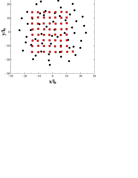
Figure 1: Snapshot of the final configuration of a system of $N=57$ electrons (filled circles) after a full QMC run (disk geometry). The system of electrons is described by an anisotropic Fermi liquid BRS wave function with $\alpha=5$ and represents a state with filling factor $\nu=1/6$ of the LLL. The initial configuration of the system at the start of the QMC run is also given (filled squares). Note that the electrons are initially placed in a regular square lattice and, then, are randomly displaced by a little bit relative to the lattice sites for better randomization before the start of a QMC run.

In our study we resort to the approximation of neglecting the LLL projection operator (LLL projection would affect the plane wave states of the Slater determinant). The kinetic energy would have been a mere constant if the whole wave function would have been properly projected kamilla . Although lack of LLL projection may affect quantitatively the energy values for a given system of electrons, it will not change qualitatively any of the main conclusions drawn since we are interested in energy differences. With other words, energy differences will likely be quite accurate (with or without LLL projection) since separately the energies are calculated within the same approximation. Hence, the discrepancies/errors which are systematic will be of the same order of magnitude and would tend to cancel out when energy differences are calculated. Earlier studies of isotropic CF wave functions (constructed by multiplying the wave functions for filled LLs with Jastrow-Laughlin correlation factors) have shown that such correlation factors ensure that the resulting states lie predominantly in the LLL trivedi . For simplicity of notation, let’s denote as $P_{N}(\nu)=\prod_{i>j}^{N}(z_{i}-z_{j})^{1/\nu}$ the Laughlin polynomial factor of an isotropic state at filling factor, $\nu$. For instance, $P_{N}(\nu=1/3)=\prod_{i>j}^{N}(z_{i}-z_{j})^{3}$ represents the typical isotropic polynomial factor of a Laughlin wave function at filling factor $\nu=1/3$ of the LLL. Note that the $\alpha$-dependent anisotropic polynomial factor in the BRS wave function of Eq.(5) can be viewed as: $P_{N}(\nu=1/6)-\alpha^{2}\,P_{N}(\nu=1/4)$. As already pointed out, each of the isotropic unprojected wave functions, separately, are expected to have tiny amplitudes in higher LLs. Since the anisotropic BRS wave function can be viewed as a linear combination of two isotropic counterparts, the conclusion reached for each isotropic portion is expected to apply to the linear combination. This means that the presence of Jastrow-Laughlin polynomial factors with relative high powers in Eq.(5) already provides a considerably projection into the LLL trivedi reassuring us on the validity of the approach.

Figure 2: Difference of energy (per electron), $\Delta\epsilon_{\alpha}=\epsilon_{\alpha}-\epsilon_{0}$ as a function of the anisotropy parameter, $\alpha$. The energy, $\epsilon_{\alpha}$ is the energy (per electron) of the anisotropic BRS liquid state while, $\epsilon_{0}$ is its isotropic liquid counterpart. Results are obtained after QMC simulations in a disk geometry for a system of $N=25$ electrons at filling factor $\nu=1/6$ of the LLL. Electrons interact with an anisotropic Coulomb interaction potential, $v_{\gamma=2}(x,y)$ where $\gamma=2$ represents the value of the interaction anisotropy parameter. Energies are in units of $e^{2}/l_{0}$.

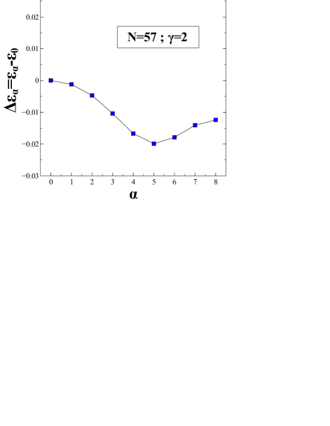
Figure 3: Same as in Fig. 2 but for a larger system of $N=57$ electrons. The energy differences for the larger system of $N=57$ electrons are very close to values seen for the smaller system of $N=25$ electrons.

It has been recently pointed out that the topological description of FQHE wave functions is not complete since the usual implicit assumption of rotational symmetry hides key geometrical features haldane2011 . Along these lines, one must distinguish between several ”metrics” that naturally arise in a real electronic system. One metric derives from the band mass tensor of electrons. A second metric is controlled by the dielectric properties of the semiconducting material that hosts the electrons haldane2011 . The second metric determines the nature of the interaction between electrons. The rotational invariance of the system is lifted if these two metrics are different from one another. What counts is the relative difference between them bo . Thus, one can, for simplicity, assume an isotropic mass tensor and anisotropic dielectric tensor. In other words, as done in this work, one can assume that the mass of electrons is isotropic, but treat the interaction between electrons as anisotropic. It turns out that, despite differences in specific details, the discussion in Sec. II, the model/treatment and the wave function considered here dovetail and are fully consistent with the spirit of Haldane’s ideas haldane2011 .

IV Results and conclusions

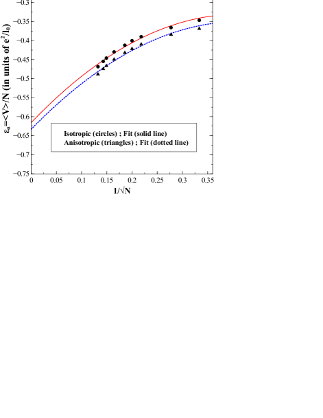
Figure 4: Monte Carlo results in disk geometry corresponding to an isotropic ($\alpha=0$) and anisotropic ($\alpha\neq 0$) Fermi liquid states at filling factor $\nu=1/6$ of the LLL. The interaction energy per electron, $\epsilon_{\alpha}=\langle\hat{V}\rangle/N$, is plotted as a function of $1/\sqrt{N}$ for systems with $N=5,9,13,21,25,29,37,49$ and $57$ electrons. Filled circles correspond to energies of isotropic states ($\alpha=0$) where the solid line is the least square fit function in Eq.(6). Filled triangles correspond to energies of anisotropic states (at optimal $\alpha_{0}\neq 0$) where the dotted line is the least square fit of Eq.(7). Electrons interact with an anisotropic Coulomb interaction potential, $v_{\gamma=2}(x,y)$. Statistical uncertainty is of the size of the symbols used. Energies are in units of $e^{2}/l_{0}$.

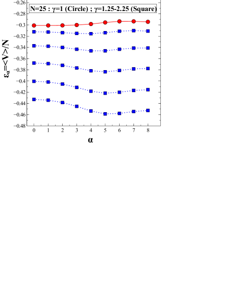
Figure 5: Energy per electron as a function of wave function anisotropy parameter, $\alpha$ for an anisotropic Coulomb interaction potential, $v_{\gamma}(x,y)$ with interaction anisotropy parameter values varying from $\gamma=1$ (standard isotropic Coulomb interaction potential) up to $\gamma=2.25$ (largest strength of the anisotropic Coulomb interaction potential considered). Filled circles correspond to $\gamma=1$ (isotropic Coulomb). Filled squares correspond to $\gamma=1.25,1.50,1.75,2.00$ and $2.25$ (from top to bottom). The system under consideration consists of $N=25$ electrons in disk geometry at filling factor $\nu=1/6$ of the LLL. The value, $\alpha=0$ represents an isotropic Fermi liquid phase. Any other value, $\alpha>0$ represents anisotropic BRS Fermi liquid states. Statistical uncertainty is of the size of the symbols used. Solid/dotted lines are guides for the eye. Energies are in units of $e^{2}/l_{0}$.

In our calculations, we consider small finite systems of electrons at filling factor $\nu=1/6$ of the LLL. The electrons are confined in a uniformly charged background disk and interact with each other via the anisotropic Coulomb interaction potential, $v_{\gamma}(x,y)$ of Eq.(4). The system of electrons under consideration is described by the BRS Fermi liquid wave function in Eq.(5). We performed detailed quantum Monte Carlo (QMC) simulations mcdisk in disk geometry in order to assess the stability of given BRS liquid crystalline phases relative to the isotropic liquid counterpart. QMC simulations enabled us to calculate accurately the potential energy (per electron), $\epsilon_{\alpha}=\langle\hat{V}\rangle/N$ for a chosen set of values of the anisotropy parameter ranging from $\alpha=0$ (isotropic) to $\alpha=8$ (the largest value considered) in steps of $1$. From now on, it is implied that values of $\alpha$ are given in units of the magnetic length, $l_{0}$. We, initially, choose an anisotropic Coulomb interaction potential with $\gamma=2$ to start the calculations. We considered various systems with $5\leq N\leq 57$ electrons. As can be seen from Fig. 1 the distribution of electrons somehow reflects the built-in anisotropy of the BRS liquid crystalline wave function. After obtaining the energies of all systems considered, we calculated the energy difference between anisotropic BRS liquid crystalline states and their isotropic liquid counterpart: $\Delta\epsilon_{\alpha}=\epsilon_{\alpha}-\epsilon_{0}$ as a function of the anisotropy parameter, $\alpha$. In Fig. 2 we show the results for $\Delta\epsilon_{\alpha}$ for a system of $N=25$ electrons where electrons interact with the anisotropic Coulomb interaction potential, $v_{\gamma=2}(x,y)$. The statistical uncertainity of the results is smaller than the size of the symbols (note that energy differences are generally very accurate). It is evident that the anisotropic BRS liquid state of electrons is energetically favored at all instances. Even though we did not try a full optimization of the energy as a function of the continuous parameter, $\alpha$, the QMC simulations clearly indicated that there is always a value $\alpha\neq 0$ (namely, there is an anisotropic liquid state of electrons) that has lower energy than the isotropic one. For the given choice of discrete, $\alpha=0,1,\ldots,8$ values, the lowest energy of a system of $N=25$ electrons was achieved for an optimal value of $\alpha_{0}=5$. For the case study of $N=25$ electrons interacting with an anisotropic Coulomb interaction, $v_{\gamma=2}(x,y)$, the amount of gain in energy was found to be approximately $\sim 20\times 10^{-3}\,{e^{2}}/{l_{0}}$ which is quite sizeable in a quantum Hall energy scale. As can be seen from Fig. 3, simulations with a larger number of $N=57$ electrons and same $v_{\gamma=2}(x,y)$ anisotropic interaction potential show similar qualitative features as those for $N=25$ electrons. This means that energy differences are almost size-independent.

In order to obtain a reasonable bulk estimate of the energy of the system in the thermodynamic limit for the $v_{\gamma=2}(x,y)$ anisotropic interaction potential, we performed a careful finite-size analysis of the available data for systems of $5\leq N\leq 57$ electrons. We followed wellknown procedures morfhalperin to fit the available energies with a quadratic polynomial function (of $1/\sqrt{N}$). This was done for both isotropic Fermi liquid states ($\alpha=0$) and anisotropic BRS liquid states (those with the lowest energy for an optimal value, $\alpha_{0}\neq 0$). For the isotropic case ($\alpha=0$), we found:

$$\epsilon_{0}=\left(-0.61565+\frac{1.38519}{\sqrt{N}}-\frac{1.68438}{N}\right)\frac{e^{2}}{l_{0}}\ .$$ (6)

The result of the fit for the optimal anisotropic BRS energies was:

$$\epsilon_{\alpha_{0}}=\left(-0.63322+\frac{1.36197}{\sqrt{N}}-\frac{1.63615}{N}\right)\frac{e^{2}}{l_{0}}\ .$$ (7)

In Fig. 4 we show the interaction energy per electron plotted as a function of $1/\sqrt{N}$ together with the results of the fit. Extrapolation of the results (for $N\rightarrow\infty$) provides a useful estimate to the energy in the thermodynamic limit (the first term in each of the parentheses). Although the convergence of the results (as a function of $N$) is slow (very typical) and we are limited by our computational power to systems with up to $N\leq 57$ electrons, the results of the extrapolation in the $N\rightarrow\infty$ limit seem unambiguous in suggesting that the lower energy of the anisotropic BRS Fermi liquid state persists in the bulk limit.

The value of the interaction anisotropy parameter, $\gamma$ is set phenomenologically. We choose to set it initially to $\gamma=2$ and the results in Fig. 2, Fig. 3 and Fig. 4 reflect this choice. This choice of $\gamma$, while not special, seems to be somewhere in the middle of the range of choices seen on related studies dealing with a similar topic. For instance, a recent work on the effect of the same anisotropic Coulomb interaction potential on the $\nu=1/3$ FQHE state employing an exact diagonalization method for $N=10$ electrons in torus geometry haowang uses values of interaction anisotropy parameter that range from $1$ (isotropic) to way larger than $4$ or $5$ (anisotropic). That said, a legitimate question that arises is whether the same behavior as seen for $\gamma=2$ persists if we use smaller values of the interaction anisotropy parameter, $\gamma$. To check the situation, we performed additional simulations for a finite system of $N=25$ electrons at filling factor $\nu=1/6$ of the LLL using different $\gamma$ values that are smaller than the initially considered value of $\gamma=2$. This way we can see whether the isotropic Fermi liquid state survives the breakdown of rotational invariance for smaller interaction anisotropy values. To this effect we considered a series of values for the interaction anisotropy parameter, $\gamma$ that vary from $1$ (isotropic Coulomb interaction potential) to $2.25$ and in between in steps of $0.25$. The results in Fig. 5 for $\gamma=1,1.25,1.50,\ldots$ and systems of $N=25$ electrons clearly show that any value $\gamma\neq 1$ considered leads to an anisotropic BRS liquid phase at filling $\nu=1/6$, while the isotropic liquid state is always stable for $\gamma=1$. The results seem to suggest that any value, $\gamma>\gamma_{c}$ where $\gamma_{c}$ is between $1$ and $1.25$ (and possibly quite close to $1$) will lead to the stabilization of an anisotropic BRS liquid state. However, a precise determination of $\gamma_{c}$ would be hard to quantify based on the numerical accuracy limitations of these calculations when calculating the expected very small energy differences between states in such limit. Since the parameter, $\alpha$ in the BRS wave function, $\Psi_{\alpha}$ is adjustable, the present calculations test the variational principle for a Hamiltonian with isotropic ($\gamma=1$) and anisotropic ($\gamma>1$) interaction. In both cases, the energy (namely, the expectation value of the quantum Hamiltonian with respect to the chosen wave function) develops a minimum. The minimum occurs at $\alpha=0$ for the isotropic ($\gamma=1$) interaction and at a nonzero value, $\alpha_{0}\neq 0$ for the anisotropic ($\gamma>1$) case. Therefore, a related question that one might want to ask is how $\alpha_{0}$ varies as $\gamma\rightarrow 1$. Hence, a study of the $\alpha$-$\gamma$ relationship in the $\gamma\rightarrow 1$ limit is of great interest. When $\gamma=1$, the value $\alpha=0$ is the natural minimum for the energy of this family of wave functions. This fact can be used to obtain a qualitative understanding of how the overlap between the $\alpha\neq 0$ and the $\alpha=0$ state varies since one can see from Eq.(5) that:

$$\Psi_{\alpha}=\Biggl{[}1-\alpha^{2}\prod_{i>j}^{N}\frac{1}{(z_{i}-z_{j})^{2}}\Biggr{]}\,\Psi_{\alpha=0}\ .$$ (8)

Apart normalization factors, one notices that $\langle\Psi_{\alpha=0}|\Psi_{\alpha}\rangle\approx 1-c\,\alpha^{2}$, where $c$ represents a constant.

When $\alpha=0$, the wave function in Eq.(5) represents an isotropic Fermi liquid state. It appears clear that, for this set of wave functions, the $\alpha=0$ BRS wave function in Eq.(5) represents the mininum energy state when electrons interact with a standard isotropic Coulomb interaction potential ($\gamma=1$). For a system of $N=25$ electrons, we found that $\epsilon_{\alpha=0}(\gamma=1)=-0.30083\,e^{2}/l_{0}$ (see Fig. 5). This energy value compares very favorably with the expected CF Wigner crystal energy at the same filling factor. The study in Ref. 38 provides a useful reference energy (that serves as a broad guideline of typical ground state energies as a function of filling factor). It is denoted as $E_{fit}$ in the caption of Fig. 2 of Ref. 38 (a figure that reflects results obtained with systems of $N=96$ electrons in spherical geometry). We used the expression for $E_{fit}$ that was provided to obtain an estimate of the expected CF crystal state energy at filling factor $\nu=1/6$ resulting in $E_{fit}(\nu=1/6)=-0.299477\,e^{2}/l_{0}$. A crude analysis of the data available, indicates further decrease of the $\epsilon_{\alpha=0}(\gamma=1)$ energy when $N$ increases. This trend is typical for systems of electrons in a disk geometry (for instance, see Fig. 4). The indication is that the $\alpha=0$ isotropic Fermi liquid state energies for the $\nu=1/6$ state of electrons interacting with a standard Coulomb interaction potential are close and lower than the $E_{fit}(\nu=1/6)$ value. However, as we already cautioned earlier in Sec. III, one should not draw any definitive conclusions since in this case we are comparing results that are obtained under different conditions, namely disk versus spherical geometry and LLL unprojected versus projected wave function (the case of the CF Wigner crystal states). What is definitely clear from our results is a substantial decrease of the energy achieved by the BRS wave function in Eq.(5) for the case of the anisotropic $v_{\gamma=2}(x,y)$ interaction potential. A useful hint that we can draw from this finding is to suggest that a ”deformed/distorted” (via the splitting of the zeroes mechanism) CF Wigner crystal state may be a better starting point to study Wigner crystal phases in the LLL for a $v_{\gamma>1}(x,y)$ anisotropic interaction potential between electrons as the one considered here.

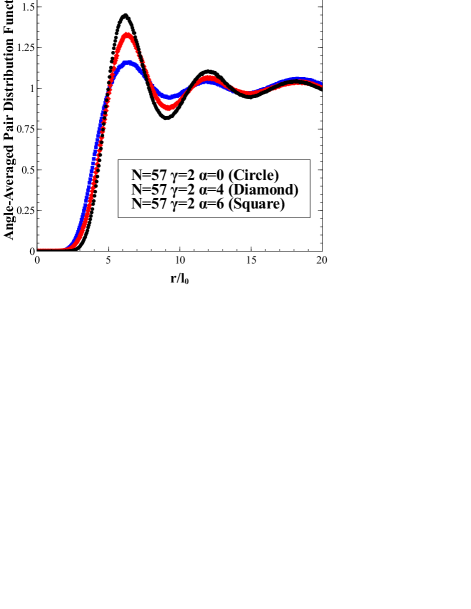
Figure 6: Angle-averaged pair distribution function, $g(r)$ as a function of dimensionless distance, $r/l_{0}$ for a system of $N=57$ electrons. The system is described by an anisotropic BRS Fermi liquid wave function for filling factor $\nu=1/6$ of the LLL. The values of the anisotropy parameter are $\alpha=0$ (Filled circle), $\alpha=4$ (Filled diamond) and $\alpha=6$ (Filled square). Note that the value $\alpha=0$ represents an isotropic Fermi liquid phase. Electrons interact with an anisotropic Coulomb interaction potential, $v_{\gamma=2}(x,y)$.

Figure 7: Angle-averaged density function, $\rho(r)/\rho_{0}$ as a function of the dimensionless distance, $r/l_{0}$ from the center of the disk for a system of $N=49$ electrons. Electrons interact with an anisotropic Coulomb interaction potential, $v_{\gamma=2}(x,y)$. The system is described by an anisotropic BRS Fermi liquid wave function for filling factor $\nu=1/6$ of the LLL. The values of the anisotropy parameter are $\alpha=0$ (Filled circle), $\alpha=4$ (Filled diamond) and $\alpha=6$ (Filled square). Note that the value $\alpha=0$ represents an isotropic Fermi liquid phase. Note the persistence of an ”edge region” of finite width at the edge of the disk. The quantity, $\rho_{0}=\nu/(2\,\pi\,l_{0}^{2})$ represents the uniform density value for the system under consideration.

There are some qualitative similarities between the $\Delta\epsilon_{\alpha}$ vs $\alpha$ dependence in the current work to an earlier study cite2011d that dealt with the possibility of an anisotropic quantum Hall liquid state at filling factor $\nu=9/2$. In that study, we considered finite systems of electrons interacting with an isotropic (though non-Coulomb) interaction potential that was properly raised in the second excited LL (the level with quantum number, $n=2$). In such an instance, we argued for the possibility of liquid crystalline phases where rotational symmetry is spontaneously broken (since the interaction potential is isotropic). We found out that the optimal value, $\alpha_{0}$ for which a minimum energy is obtained tends to be size-dependent for the $\nu=9/2$ state. It was $\alpha_{0}\approx 4$ for a system of $N=5$ electrons, it became $\alpha_{0}\approx 3$ for $N=13$ electrons and eventually stabilized to the value $\alpha_{0}\approx 2$ for the largest systems considered ($21\leq N\leq 49$). We attributed the variations of $\alpha_{0}$ for small systems ($5\leq N\leq 13$) to the small size and ”edge” effects. However, we argued that the optimal value $\alpha_{0}=2$ is not casual. In fact we suggested that the optimal choice, $\alpha_{0}=2$ for the $\nu=9/2$ state is approximately set by the location of the dominant cusp of the $v_{n=2}(r)$ potential which represents the effective interaction potential between electrons in the upper LL with quantum number $n=2$ that is half-filled cite2011d . We remind the reader that the interaction potential, $v_{n=2}(r)$ is isotropic but non-monotonic (has cusps). It can be exactly calculated in real space orionjltp . It differs substantially from an isotropic and/or anisotropic Coulomb interaction potential (like the one in the current work) for all excited LLs where $n\geq 1$.

For the case of the anisotropic Coulomb interaction potential, $v_{\gamma=2}(x,y)$ we found out that, except for the smallest of the systems of electrons considered ($N=5$), the lowest energy of an anisotropic state is achieved for $\alpha_{0}=5$ in all other cases ($9\leq N\leq 57$). Specifically speaking, the results for the $v_{\gamma=2}(x,y)$ interaction potential indicate that the optimal value, $\alpha_{0}$ shows some size-dependence for the smallest systems considered, but then quickly settles to $\alpha_{0}\approx 5$ when the system size increases. It is hard to tell if this value is hinting at something of significance. Generally speaking, we would argue that the optimal choice for $\alpha_{0}$ is set by the strength of the interaction anisotropy parameter, $\gamma$. It is very tempting to say that the optimal value, $\alpha_{0}$ is set by the ratio $v_{\gamma}(x,y=0)/v_{\gamma}(x=0,y)\propto\gamma^{2}$ for $|x|\approx|y|$ but this appears to be too crude. Nevertheless, this statement might still bear some truth since simulations with $N=25$ electrons indicate that the optimal choice, $\alpha_{0}$ decreases when $\gamma$ decreases. For instance, our simulation results for $N=25$ electrons indicate that the optimal value is $\alpha_{0}=4$ for $v_{\gamma=1.25}(x,y)$ and $v_{\gamma=1.50}(x,y)$ interaction potentials. However, as can also be seen from the results in Fig. 5, the value $\alpha_{0}$ increases to $\alpha_{0}=5$ for $v_{\gamma=1.75}(x,y)$, $v_{\gamma=2.00}(x,y)$, and $v_{\gamma=2.25.}(x,y)$ interaction potentials. As previously stated, we use only values, $\alpha=0,1,\ldots,8$ in our calculations. In Fig. 6 we plot the angle-averaged pair distribution function, $g(r)=\int_{0}^{2\,\pi}\frac{d\,\theta}{2\,\pi}\,g(r,\theta)$ for $\alpha=0,4$ and $6$ corresponding to a system of $N=57$ electrons, the largest that we were able to consider. One notices that the major peak of $g(r)$ becomes less pronounced and very slightly shifts to larger values of $r$ as $\alpha$ increases. The short-range behavior of the $g(r)$ also changes as $\alpha$ increases. We found that $g(r)$ changes from approximately $\propto r^{14}$ ($\alpha=0$) to approximately $\propto r^{10}$ ($\alpha\neq 0$). Such a shift is expected from general considerations of the nature of the magnitude square of the wave function at small separation distances between electrons. The differences in the $g(r)$-s may also be the result of different correlations in different directions canceling. In Fig. 7 we plot the angle-averaged density function, $\rho(r)=\int_{0}^{2\,\pi}\frac{d\,\theta}{2\,\pi}\,\rho(r,\theta)$ relative to its uniform density value, $\rho_{0}$ as a function of the dimensionless distance parameter, $r/l_{0}$ for several BRS wave functions with different values of the anisotropy parameter, $\alpha$. The density function seems to be sensitive to the wave function parameters in the central region of the disk, but less at the edge. This might be an indication of interesting topological quantum Hall edge effects ijmpb2012 where anisotropy might play some subtle role.

Another way to incorporate the effects of anisotropy into a typical quantum Hall wave function is through appropriate modifications of the CF theory. For instance, one can write a family of microscopic CF wave functions that incorporate electron mass anisotropy by a rescaling of the electron coordinates balram . In this model one starts with electrons that have anisotropic mass ($m_{x}\neq m_{y}$) and then sets up the single-particle particle states in terms of complex coordinates that depend on a mass anisotropy parameter (with $x$ and $y$ coordinates scaled differently). The resulting CF wave functionn is anisotropic since in this approach the single-particle states are anisotropic by construction. The problem of electrons with anisotropic mass interacting with an isotropic Coulomb interaction potential is effectively equivalent to the problem of electrons with isotropic mass interacting with an anisotropic Coulomb interaction potential as the one considered in our work. Thus, we are basically dealing with the some problem despite apparent differences in formalism, namely, the interaction anisotropy parameter $\gamma$ of the $v_{\gamma}(x,y)$ potential may be interpreted as a mass anisotropy parameter in the anisotropic CF approach of systems of electrons interacting via the usual isotropic Coulomb interaction potential. At this juncture, apart from the fact that we are looking at different filling factors, it is important to remark a striking difference between the wave function in Eq.(5) and the anisotropic CF wave functions already mentioned balram . Anisotropy in our case is introduced at the two-body level of the wave function while anisotropy originates from single-particle states within the anisotropic CF wave function framework.

It is interesting to point out that small-$N$ results for anisotropic CF states at Laughlin filling factor $\nu=1/3$ seem to suggest that energy is very insensitive to anisotropy for up to fairly large values of the effective mass/interaction anisotropy parameter balram . Our calculations for the Fermi liquid state at filling factor $\nu=1/6$ pursue a different avenue, but seem to indicate that the energy of the $\nu=1/6$ state is quite sensitive to the increasing anisotropy at least for the specific choice of the wave function that we made. Absence of an energy gap for the $\nu=1/6$ Fermi liquid state under consideration might suggest that such a state is easily deformable and, thus, might be prone to destabilization. If there is some truth in this statement, a more general hint comes from this behavior, namely, all the other Fermi liquid states in the LLL might show similar tendencies since all Fermi liquid states at filling factors of the form $\nu=1/2$, $1/4$ and $1/6$ share similar characteristics. Thus, one might be tempted to say that all even-denominator filled Fermi liquid states in the LLL (including the ones at $\nu=1/2$ and $\nu=1/4$) might be prone to destabilization by an anisotropic Coulomb interaction of the form considered here through the same mechanism.

To conclude, in this work we introduced the idea that the impact of a weak anisotropic electron-electron interaction perturbation possibly originating from the piezoelectric property of the GaAs substrate may stabilize novel electronic liquid crystalline phases even in the LLL. In particular, we envisioned the possibility that the very fragile isotropic Fermi liquid state at filling factor $\nu=1/6$ of the LLL can be destabilized by an electron-electron anisotropic perturbation. Our calculations suggest that this happens for the case of a phenomenological anisotropic Coulomb interaction potential, $v_{\gamma}(x,y)$ at all values of the interaction anisotropy parameter we considered ($1.25\leq\gamma\leq 2.25$) for all the sizes of the finite systems of electrons that we considered ($5\leq N\leq 57$). Our finite QMC results suggest the stabilization of a novel anisotropic liquid crystalline phase of electrons due to anisotropy whose experimental signatures may be detectable at ultra-low temperatures of order $1\,mK$. It is conjectured that the same tendency toward liquid crystalline order in presence of an anisotropic interaction potentional may be observed at other known even-denominator filled Fermi liquid states in the LLL (for instance, $\nu=1/2$ and $1/4$).

- (1) O. Ciftja, J. Math. Phys. 52, 122105 (2011).
- (2) D. C. Tsui, H. L. Stormer, and A. C. Gossard, Phys. Rev. Lett. 48, 1559 (1982).
- (3) R. L. Willett, M. A. Paalanen, R. R. Ruel, K. W. West, L. N. Pfeiffer, and D. J. Bishop, Phys. Rev. Lett. 65, 112 (1990).
- (4) R. L. Willett, R. R. Ruel, M. A. Paalanen, K. W. West, and L. N. Pfeiffer, Phys. Rev. B. 47, 7344 (1993).
- (5) P. K. Lam and S. M. Girvin, Phys. Rev. B 30, 473(R) (1984).
- (6) K. Esfarjani and S. T. Chui, Phys. Rev. B 42, 10758 (1990).
- (7) X. Zhu and S. G. Louie, Phys. Rev. B 52, 5863 (1995).
- (8) R. B. Laughlin, Phys. Rev. Lett. 50, 1395 (1983).
- (9) J. K. Jain, Phys. Rev. Lett. 63, 199 (1989).
- (10) O. Ciftja, Physica E 9, 226 (2001).
- (11) O. Ciftja, Eur. Phys. J. B 13, 671 (2000).
- (12) B. I. Halperin, P. A. Lee, and N. Read, Phys. Rev. B 47, 7312 (1993).
- (13) E. Rezayi and N. Read, Phys. Rev. Lett. 72, 900 (1994).
- (14) O. Ciftja and S. Fantoni, Phys. Rev. B 58, 7898 (1998).
- (15) M. P. Lilly, K. B. Cooper, J. P. Eisenstein, L. N. Pfeiffer, and K. W. West, Phys. Rev. Lett. 82, 394 (1999).
- (16) M. M. Fogler, A. A. Koulakov, and B. I. Shklovskii, Phys. Rev. B 54, 1853 (1996).
- (17) R. Moessner and J. T. Chalker, Phys. Rev. B 54, 5006 (1996).
- (18) E. Fradkin and S. A. Kivelson, Phys. Rev. B 59, 8065 (1999).
- (19) V. Oganesyan, S. A. Kivelson, and E. Fradkin, Phys. Rev. B 64, 195109 (2001).
- (20) Q. M. Doan and E. Manousakis, Phys. Rev. B 75, 195433 (2007).
- (21) O. Ciftja and C. Wexler, Phys. Rev. B 65, 205307 (2002).
- (22) C. Wexler and O. Ciftja, Int. J. Mod. Phys. B 20, 747 (2006).
- (23) O. Ciftja, J. Appl. Phys. 107, 09C504 (2010).
- (24) O. Ciftja, B. Cornelius, K. Brown, and E. Taylor, Phys. Rev. B 83, 193101 (2011).
- (25) K. B. Cooper, M. P. Lilly, J. P. Eisenstein, L. N. Pfeiffer, and K. W. West, Phys. Rev. B 65, R241313 (2002).
- (26) T. Jungwirth, A. H. MacDonald, L. Smrčka, and S. M. Girvin, Phys. Rev. B 60, 15574 (1999).
- (27) T. Stanescu, I. Martin, and P. Phillips, Phys. Rev. Lett. 84, 1288 (2000).
- (28) M. P. Lilly, K. B. Cooper, J. P. Eisenstein, L. N. Pfeiffer, and K. W. West, Phys. Rev. Lett. 83, 824 (1999).
- (29) W. Pan, T. Jungwirth, H. L. Stormer, D. C. Tsui, A. H. MacDonald, S. M. Girvin, L. Smrčka, L. N. Pfeiffer, K. W. Baldwin, and K. W. West, Phys. Rev. Lett. 85, 3257 (2000).
- (30) J. Xia, J. P. Eisenstein, L. N. Pfeiffer, and K. West, Nat. Phys. 7, 845 (2011).
- (31) O. Ciftja, C. M. Lapilli, and C. Wexler, Phys. Rev. B 69, 125320 (2004).
- (32) A. J. Schmidt, O. Ciftja, and C. Wexler, Phys. Rev. B 67, 155315 (2003).
- (33) K. Yang, F. D. M. Haldane, and E. H. Rezayi, Phys. Rev. B 64, 081301(R) (2001).
- (34) O. Ciftja, Europhys. Lett. 74, 486 (2006).
- (35) O. Ciftja, B. Sutton, and A. Way, AIP Advances 3, 052110 (2013).
- (36) K. Musaelian and R. Joynt, J. Phys. Cond. Matter 8, L105 (1996).
- (37) O. Ciftja, J. Low. Temp. Phys. 183, 85 (2016).
- (38) A. C. Archer, K. Park, and J. K. Jain, Phys. Rev. Lett. 111, 146804 (2013).
- (39) R. K. Kamilla and J. K. Jain, Phys. Rev. B 55, 9824 (1997).
- (40) N. Trivedi and J. K. Jain, Mod. Phys. Lett. B 05, 503 (1991).
- (41) F. D. M. Haldane, Phys. Rev. Lett. 107, 116801 (2011).
- (42) B. Yang, Z. Papić, E. H. Rezayi, R. N. Bhatt, and F. D. M. Haldane, Phys. Rev. B 85, 165318 (2012).
- (43) O. Ciftja and C. Wexler, Phys. Rev. B 67, 075304 (2003).
- (44) R. Morf and B. I. Halperin, Phys. Rev. B. 33, 2221 (1986).
- (45) H. Wang, R. Narayanan, X. Wan, and F. Zhang, Phys. Rev. B 86, 035122 (2012).
- (46) O. Ciftja and J. Quintanilla, J. Low. Temp. Phys. 159, 189 (2010).
- (47) O. Ciftja, Int. J. Mod. Phys. B 26, 1244001 (2012).
- (48) A. C. Balram and J. K. Jain, Phys. Rev. B 93, 075121 (2016).