Criterion for Stability of a Special Relativistically Covariant Dynamical System

Abstract

We study classically the problem of two relativistic particles with an invariant Duffing-like potential which reduces to the usual Duffing form in the nonrelativistic limit. We use a special relativistic generalization (RGEM) of the geometric method (GEM) developed for the analysis of nonrelativistic Hamiltonian systems to study the local stability of a relativistic Duffing oscillator. Poincaré plots of the simulated motion are consistent with the RGEM. We find a threshold for the external driving force required for chaotic behavior in the Minkowski spacetime.

I Introduction

In Newton’s classical mechanics and in quantum mechanics, one makes use of a global time that has causal meaning. The manifestly covariant Stueckelberg formalism Stueckelberg:1941rg ,17.horwitz1973relativistic is based on a similar idea, that there is an invariant parameter $\tau$ of evolution of the system.

According to Stueckelberg, covariant functions of space and time (Einstein’s time, $t$) form a Hilbert space (over $R^{4}$) for each value of $\tau$ (which we shall refer to as “world time”). Thus, there are two types of time, one transforming covariantly, and the second an invariant parameter of evolutionhorwitz2015relativistic . The first type, Einstein’s time in the theory of relativity, $t$, of an event as measured in the laboratory is subject to variation (Lorentz transformation) according to the velocity of the apparatus related to the transmitting system and may as well be affected by forces (such as gravity), and the second type is the Stueckelberg’s world time, $\tau$, that remains unaffected horwitz1988two .

This allows us to write equations of motion for a single particle that depend on the world time $\tau$, in terms of Hamilton equations based on a Hamilton function of $x,p$ in the quantum theory where $x,p$ are covariant four-vectors. The dynamics of the system is driven by $\tau$; $t$ and $x$ are quantities that are observed in the laboratory. The Maxwell equations, for examples, describe electromagnetic phenomena in terms of the observable $t$ and $x$, but. in Stueckelberg’s framework, the sources (with spacetime positions given by $x$ and $t$) are governed by equations of motion in $\tau$, as discussed in detail in 17.horwitz1973relativistic . The results of our analysis therefore describe the physically observable consequences of the dynamical evolution. consequences of the dynamical evolution.

As done by Stueckelberg, one can write a Schr$\ddot{o}$dinger type equation for the wave function for a free particle (for $\mu=0,1,2,3$):

$$i\frac{\partial}{\partial\tau}\psi_{\tau}(x^{\mu})=\eta_{\mu\nu}\frac{p^{\mu}p^{\nu}}{2M}\psi_{\tau}(x^{\mu}),$$

where $x^{\mu}=x(x,t)$, $\eta_{\mu\nu}=diag(-1,1,1,1)$ and $\tau$ is the invariant parameter of evolution. M is a parameter of dimension mass (but not the measured or the rest mass; it may be considered the Galilean (nonrelativistic) limit mass 11.horwitz1981gibbs ). One sees that for the classical case by the Hamilton equations

$$\dot{x}^{\mu}\equiv\frac{dx^{\mu}}{d\tau}=\frac{p^{\mu}}{M}=\frac{\partial H}{\partial p_{\mu}}$$

so that

$$-\frac{ds^{2}}{d\tau^{2}}=\frac{dx^{\mu}dx_{\mu}}{d\tau^{2}}=-\frac{m^{2}}{M^{2}}$$

where $m$ is the measured mass and $s$ is the proper time. Therefore, the proper time coincides with with $\tau$ when $m=M$ (called the "mass shell").

To describe the dynamical evolution of a more than one particle system, Horwitz and Piron generalized Stueckelberg’s theory and postulated a universal $\tau$ for any number of particles, enabling the solution of the two body problem in particular. They separated variables to CM (center of four-mometnum frame variables) and relative motion, and solved the classical Kepler problem with invariant potential proportional to $1/\rho$, where $\rho=\sqrt{x^{2}-t^{2}}$, with $x,t$ relative coordinates. Arshansky and Horwitz 12.arshansky1989quantum1 , reduced the relativistic quantum problem to the corresponding nonrelativistic Schr$\ddot{o}$dinger equation with $V(\rho)$, where $\rho$ replaces the radial coordinate r everywhere in the equation. The solutions they found were irreducible representations of O(2,1) and they therefore introduced an induced representation to obtain representations of O(3,1) 13.arshansky1989quantum2 .

Horwitz and Schieve treated the reduced motion of a relativistic Duffing oscillator with a potential of the form

$$V(\rho)=a\rho^{4}-b\rho^{2}+c$$

where $\rho^{2}=x^{\mu}x_{\mu}$, by simulation.

In this work, we generalize the method of Horwitz et al 14.horwitz2007geometry (called GEM) for studying the stability of nonrelativistic Hamiltonian systems to the relativistic case (which we shall call RGEM), and use both methods, simulation and the application of the RGEM criterion to study the stability of the relativistic Duffing oscillator.

It will be shown here that the unstable orbits found by Schieve and Horwitz pass through the regions of instability indicated by the GEM criterion generalized to the relativistic (RGEM) case and that the occurrence of chaos on Poincaré plots and on the space time orbits. The formula for the relativistic generalization is derived here. This application is the first that has been carried out for the relativistic form of this criterion.

II Review of Nonrelativistic Stability Theory

It has been shown 13.arshansky1989quantum2 that a Hamiltonian of standard form in nonrelativistic mechanics $(fori,j,k=1,2,3)$:

$$H=\frac{1}{2M}\eta_{\text{ij}}p^{i}p^{j}+V(y)$$ (1)

can be cast 14.horwitz2007geometry into a geometrical form 15.gutzwiller2013chaos (a method which we call GEM):

$$\hat{H}=\frac{1}{2M}g_{\text{ij}}p^{i}p^{j}$$ (2)

where $g_{ij}=\phi(x)\delta_{ij}$ (we shall call the variable of the curved space manifold $x_{i}$ to distinguish from the Hamilton space designated here by$y^{i}$).

The Hamilton equations applied to (2) imply the geodesic equation (a local diffeomorphism covariant form)

$$\ddot{x}_{i}=-\Gamma_{i}^{jk}\dot{x}_{j}\dot{x}_{k}$$ (3)

where

$$\Gamma_{i}^{jk}=\frac{1}{2}g_{im}(\frac{\partial g^{mk}}{\partial x_{j}}+\frac{\partial g^{jm}}{\partial x_{k}}-\frac{\partial g^{jk}}{\partial x_{m}})$$ (4)

A mapping in the tangent space defined by

$$\dot{x}_{i}=g_{ij}(x)\dot{y}^{j}$$ (5)

puts this equation into the (also) diffeomorphism covariant form

$$\ddot{y}^{i}=-\frac{1}{2}g^{ij}\frac{\partial g_{kl}}{\partial y^{j}}\dot{y}^{k}\dot{y}^{l}\equiv-M_{kl}^{i}\dot{y}^{k}\dot{y}^{l}$$ (6)

In the special coordinate system (for $H=\hat{H}=E$) for which $g_{ij}=\phi\delta_{ij}$,$\phi=E/(E-V)$, this equation reduces to:

$$\ddot{y}^{j}=-\frac{\partial V(y)}{\partial y^{j}},$$ (7)

and therefore recovers the usual Hamiltonian evolution.

We shall identify the variables $y^{i}$with the Hamiltonian variable, since they constitute in (6) an embedding of the actual Hamilton motion into a curved space.

As a measure of stability, the geodesic deviation derived from this is given by

$$\frac{D^{2}\zeta^{i}}{D\tau^{2}}=R_{jkl}^{i}\dot{y}^{\text{j}}\dot{y}^{l}\zeta^{k},$$ (8)

where $R_{jkl}^{i}$ is a curvature associated with the geodesic motion, turns out to be a very sensitive and reliable criterion for the stability of the original system16.zion2008applications . In this work, we generalize this procedure to the relativistic case.

III The relativistic Hamiltonian and its transformation to geometric form

Let us consider a Hamiltonian in Minkowski space of the form:

$$H=\eta_{\mu\nu}\frac{p^{\mu}p^{\nu}}{2M}+V(y)$$ (9)

where $\eta_{\mu\nu}$ is the Minkowski metric and the manifold is described in the $y$-coordinate system by our definition.

A Hamiltonian of this kind is assumed by Stueckelberg stueckelberg1993helv, who formulated the basic dynamics for both classical and quantum theory. Horwitz and Piron 17.horwitz1973relativistic generalized the theory to be applicable to the many body problem, by defining the parameter $\tau$ as universal, and worked out the two body Kepler case as an example. The quantum two body problem with invariant action at a distance potential was solved by Horwitz and Arshansky 18.arshansky1988solutions .

Our goal is to check the stability of the system by applying a conformal transformation on the metric and writing the Hamiltonian in a curved space (as done for the nonrelativistic case in 14.horwitz2007geometry ; see also Gershon and Horwitz 19.gershon2009kaluza ).

To do so, we will first write an "equivalent" Hamiltonian in curved space with no potential 20.misner1973gravitation :

$$\hat{H}=g_{\mu\nu}\frac{p^{\mu}p^{\nu}}{2M}$$ (10)

where $g_{\mu\nu}$ is the metric of the new manifold which we will describe in a coordinate manifold which we shall call ${x}$; to establish the equivalence, we require $p^{\mu}(\tau)$ to be the same in both systems. We define this dynamical equivalence on the basis that the measureable quantities $p^{\mu}$, associated with forces, should be the same at every stage of the evolution governed by $\tau$; it enables the definition of the conformal map 14.horwitz2007geometry between $(1)$ and $(2)$, shown to be highly effective in the nonrelativistic case.

In order to construct a relation between $H$ and $\hat{H}$, let us define a conformal transformation on the metric, i.e. (on the manifold ${x}$)

$$g_{\mu\nu}=\phi(x)\eta_{\mu\nu}$$ (11)

We shall assume the “energy” $E$ (value of $H$) to be equal for both systems and a correspondence between the $x$’s and $y$’s so that:

$$E=\eta_{\mu\nu}\frac{p^{\mu}p^{\nu}}{2m}+V(y)=g_{\mu\nu}(x)\frac{p^{\mu}p^{\nu}}{2M}$$ (12)

consequently:

$$\phi(x)=\frac{E}{E-V(y)}$$ (13)

for the corresponding points $x$ and $y$.

It follows from the requirement of equal momentum that (the dot corresponds to differentiation with respect to $\tau$):

$$\dot{y}^{\mu} = g^{\mu\nu}(x)\dot{x}_{\nu}$$ (14)

$$\dot{x}_{\nu} = g_{\mu\nu}(x)\dot{y}^{\mu}$$ (15)

so that:

$$\ddot{y}^{\mu}=\frac{\partial g^{\mu\nu}}{\partial\tau}\dot{x}_{\nu}+g^{\mu\nu}\ddot{x}_{\nu}\\$$ (16)

and also, by the Hamilton equations derived from (9) 15.gutzwiller2013chaos ,14.horwitz2007geometry

$$\ddot{x}_{\alpha}=-\frac{1}{2}g_{\alpha\nu}(\frac{\partial g^{\nu\theta}}{\partial x_{\lambda}}+\frac{\partial g^{\theta\nu}}{\partial x_{\lambda}}-\frac{\partial g^{\lambda\theta}}{\partial x_{\nu}})\dot{x}_{\lambda}\dot{x}_{\theta}=-\Gamma_{\alpha}^{\lambda\theta}\dot{x}_{\lambda}{\dot{x}}_{\theta}$$ (17)

so that:

$$\ddot{y}_{\nu}=\frac{1}{2}\frac{\partial g^{\lambda\theta}}{\partial x_{\nu}}g_{\rho\lambda}g_{\sigma\theta}\dot{y}^{\rho}\dot{y}^{\sigma}\equiv-M_{\rho\sigma}^{\mu}\dot{y}^{\rho}\dot{y}^{\sigma}$$ (18)

We remark that since ${y}$ corresponds to a manifold different from ${x}$ (through the mapping (14)), we have called the corresponding connection form $M_{\rho\sigma}^{\mu}$.

Now let us define the deviation between two orbits by

$$\zeta{}^{\alpha} = y^{\prime\alpha}-y^{\alpha}$$ (19)

$$y^{\prime\alpha} = y^{\alpha}+\zeta^{\alpha}$$ (20)

so that

$$\ddot{y}^{\prime\nu}=-M^{{}^{\prime}}{}_{\rho\sigma}^{\nu}\dot{y}^{\prime\rho}\dot{y}^{\prime\sigma}$$ (21)

where:

$$M^{{}^{\prime}}{}_{\rho\sigma}^{\nu}=M_{\rho\sigma}^{\nu}+\partial_{\alpha}(M_{\rho\sigma}^{\nu})\zeta^{\alpha}$$ (22)

and:

$$\partial_{\alpha}=\frac{\partial}{\partial y^{\alpha}}$$ (23)

Through the definition (13),$M_{\rho\sigma}^{\nu}$ is explicitly a function of $y^{\alpha}$.

Now, expanding up to first order in $\zeta$, $\dot{\zeta}$ we get:

$$\ddot{\zeta}^{\nu}=-2M{}_{\rho\sigma}^{\nu}\dot{y}{}^{\rho}\dot{\zeta}^{\sigma}-\partial_{\alpha}(M{}_{\rho\sigma}^{\nu})\dot{y}{}^{\rho}\dot{y}{}^{\sigma}\zeta^{\alpha}$$ (24)

If $\zeta$ is small enough, we can treat it as a tensor, and its covariant derivative is:

$$\frac{D\zeta^{\nu}}{D\tau}=\dot{\zeta}^{\nu}+M{}_{\rho\sigma}^{\nu}\dot{y}^{\rho}\zeta^{\sigma}$$ (25)

The second covariant derivative is

$$\frac{D^{2}\zeta^{\nu}}{D\tau^{2}}=\frac{d}{d\tau}(\dot{\zeta}^{\nu}+M{}_{\rho\sigma}^{\nu}\dot{y}^{\rho}\zeta^{\sigma})+M{}_{\alpha\beta}^{\nu}(\dot{\zeta}^{\alpha}+M{}_{\rho\sigma}^{\alpha}\dot{y}^{\rho}\zeta^{\sigma})\dot{y}^{\beta}\\$$ (26)

Substituting (24) into (26), we get

$$\frac{D^{2}\zeta^{\nu}}{D\tau^{2}} = -\partial_{\alpha}(M{}_{\rho\sigma}^{\nu})\dot{y}{}^{\rho}\dot{y}{}^{\sigma}\zeta^{\alpha}+\partial_{\alpha}(M{}_{\rho\sigma}^{\nu})\dot{y}^{\alpha}\dot{y}^{\rho}\zeta^{\sigma}$$ (27)

$$+ M{}_{\rho\sigma}^{\nu}\ddot{y}^{\rho}\zeta^{\sigma}+M{}_{\alpha\beta}^{\nu}M{}_{\rho\sigma}^{\alpha}\dot{y}^{\beta}\dot{y}^{\rho}\zeta^{\sigma}$$

Now inserting (18) into (27) and changing contracted indices we get:

$$\frac{D^{2}\zeta^{\nu}}{D\tau^{2}}=R_{\beta\sigma\rho}^{\nu}\dot{y}^{\beta}\dot{y}^{\rho}\zeta^{\sigma}$$ (28)

where $R$ is a "dynamical curvature" associated with the geodesic motion (18), i.e;

$$R_{\mu\nu\sigma}^{\alpha}=\frac{\partial M_{\mu\nu}^{\alpha}}{\partial y^{\sigma}}-\frac{\partial M_{\mu\sigma}^{\alpha}}{\partial y^{\nu}}+M_{\mu\nu}^{\lambda}M_{\sigma\lambda}^{\alpha}-M_{\mu\sigma}^{\lambda}M_{\nu\lambda}^{\alpha}$$ (29)

In the special coordinate system in which (13) is valid

$$R_{\mu\sigma\nu}^{\alpha}=\eta^{\alpha\kappa}[\frac{1}{2\phi(y)}(\eta_{\nu\mu}\frac{\partial^{2}\phi(y)}{\partial y^{\sigma}\partial y^{\kappa}}-\eta_{\sigma\mu}\frac{\partial^{2}\phi(y)}{\partial y^{\nu}\partial y^{\kappa}})$$

$$-\frac{1}{4\phi^{2}(y)}(\eta_{\mu\nu}\frac{\partial\phi(y)}{\partial y^{\sigma}}\frac{\partial\phi(y)}{\partial y^{\kappa}}-\eta_{\sigma\mu}\frac{\partial\phi(y)}{\partial y^{\nu}}\frac{\partial\phi(y)}{\partial y^{\kappa}})]$$ (30)

Using (13), we can calculate the first and second derivatives of $\phi(y)$ and consequently we can calculate R explicitly:

$$R_{\mu\nu\sigma}^{\alpha}=$$ (31)

$$\eta^{\alpha\kappa}[\frac{3}{4(E-V(y))^{2}}(\eta_{\mu\nu}\frac{\partial V(y)}{\partial y^{\sigma}}\frac{\partial V(y)}{\partial y^{\kappa}}-\eta_{\sigma\mu}\frac{\partial V(y)}{\partial y^{\nu}}\frac{\partial V(y)}{\partial y^{\kappa}})$$

$$+\frac{1}{2(E-V(y))}(\eta_{\mu\nu}\frac{\partial^{2}V(y)}{\partial y^{\sigma}\partial y^{\kappa}}-\eta_{\sigma\mu}\frac{\partial^{2}V(y)}{\partial y^{\nu}\partial y^{\kappa}})]$$

from (9), we have

$$E-V(y) = \eta_{\mu\nu}\frac{p^{\nu}p^{\nu}}{2m}=\frac{p^{2}}{2M}$$ (32)

We also know from the Hamilton equations that

$$\dot{y}^{\mu}=\frac{\partial H}{\partial p_{\mu}}=\frac{1}{M}p^{\mu}$$ (33)

Substituting (32) and (33) into (31),and after contracting $\mu$ and $\sigma$, the geodesic deviation equation then reads:

$$\eta_{\alpha\kappa}\frac{D^{2}\zeta^{\alpha}}{D\tau^{2}}=$$

$$[\eta_{\mu\nu}(\frac{3}{M^{2}\dot{y}^{2}}\frac{\partial V(y)}{\partial y^{\sigma}}\frac{\partial V(y)}{\partial y^{\kappa}}+\frac{1}{M}\frac{\partial^{2}V(y)}{\partial y^{\sigma}\partial y^{\kappa}})\frac{\dot{y}^{\mu}\dot{y}^{\sigma}}{\dot{y}^{2}}$$

$$-(\frac{3}{M^{2}\dot{y}^{2}}\frac{\partial V(y)}{\partial y^{\nu}}\frac{\partial V(y)}{\partial y^{\kappa}}+\frac{1}{M}\frac{\partial^{2}V(y)}{\partial y^{\nu}\partial y^{\kappa}})]\zeta^{\nu}$$ (34)

Let us define

$$Q_{\sigma\kappa}=\frac{3}{M^{2}\dot{y}^{2}}\frac{\partial V(y)}{\partial y^{\sigma}}\frac{\partial V(y)}{\partial y^{\kappa}}+\frac{1}{M}\frac{\partial^{2}V(y)}{\partial y^{\sigma}\partial y^{\kappa}}$$ (35)

and the projection (orthogonal to ${\dot{p}}^{\mu}$)

$$p_{\nu}^{\sigma}=(\eta_{\nu}^{\sigma}-\eta_{\mu\nu}\frac{\dot{y}^{\mu}\dot{y}^{\sigma}}{\dot{y}^{2}}).$$ (36)

we can then write

$$\ \eta_{\alpha\kappa}\frac{D^{2}\zeta^{\alpha}}{D\tau^{2}} = -p_{\nu}^{\sigma}Q_{\sigma\kappa}\zeta^{\nu}$$ (37)

We wish to project the deviation on the direction orthogonal to ${\dot{y}}^{\mu}$. We then obtain

$$p_{\alpha}^{\gamma}\frac{D^{2}\zeta^{\alpha}}{D\tau^{2}} = -(p_{\alpha}^{\gamma}Q_{\sigma}^{\alpha}p_{\nu}^{\sigma})\zeta^{\nu}$$ (38)

If the eigenvalues of $Q_{\sigma}^{\alpha}$ are positive, then the eigenvalues of $p_{\alpha}^{\gamma}Q_{\sigma}^{\alpha}p_{\nu}^{\sigma}$ are positive as well, so that if both of the eigenvalues of $Q_{\sigma}^{\alpha}$ are positive, then the system is stable. If either or both of the eigenvalues are negative, then the system may be considered unstable. In this case, there could be an exponentially rapid divergence of neighboring trajectories, charfacteristic of local instability. A zero eigenvalue may be considered as indicating instability as well, since a small additional perturbation may render it negative.

IV The Duffing Oscillator

We now choose a potential of the form of the invariant relativistic Duffing oscillator 23.schieve1991chaos :

$$\centering V(y)=ay^{4}-by^{2}+c,\@add@centering$$ (39)

where $y^{\mu}=y_{1}^{\mu}-y_{2}^{\mu}$, the relative coordinates of the two body system and we take $c=0$ in this study.

We shall study this problem for the 1+1 dimensional case. As we have seen, stability depends on the eigenvalues of the resulting matrix obtained by projecting the left hand side also in the direction orthogonal to the trajectory. Inserting (39) into (35) will result in the following symmetric matrix of the form:

$$Q=\left[\begin{array}[]{cc}A&B\\ B&C\end{array}\right]$$ (40)

where

$$A = -(\frac{3}{M^{2}\dot{y}^{2}}(4ay^{2}-2b)^{2}+\frac{1}{M}8a)y^{0}y_{0}$$ (41)

$$+\frac{1}{M}(4ay^{2}-2b)$$

$$B = (\frac{3}{M^{2}\dot{y}^{2}}(4ay^{2}-2b)^{2}+\frac{1}{M}8a)y_{1}y^{0}$$ (42)

$$C = (\frac{3}{M^{2}\dot{y}^{2}}(4ay^{2}-2b)^{2}+\frac{1}{M}8a)y^{1}y_{1}$$ (43)

$$+\frac{1}{M}(4ay^{2}-2b)$$

In the general case of a symmetric matrix of this form the eigenvalues are:

$$\lambda_{1,2}=\frac{(A+C)\pm\sqrt{(A+C)^{2}+4(B^{2}-AC)}}{2}$$ (44)

Since the eigenvalues of a real symmetric matrix are real, we obtain two conditions which the matrix elements must meet in order for both eigenvalues to be positive:

1. $(A+C)>0$

2. $4(B^{2}-AC)<0$

If the one of the conditions fails then at least one of the eigenvalues is negative.

The first condition gives is:

$$(\frac{3}{M^{2}\dot{y}^{2}}(4ay^{2}-2b)^{2}+\frac{1}{M}8a)y^{2}+\frac{2}{M}(4ay^{2}-2b)>0$$ (45)

Using (32) and (33) we can write the first condition explicitly:

$$(\frac{3}{8(E-V(y))}(4ay^{2}-2b)^{2}+4a)y^{2}>b$$ (46)

The second condition gives:

$$\frac{1}{M}(4ay^{2}-2b)(\frac{3}{M^{2}\dot{y}^{2}}(4ay^{2} -2b)^{2}+\frac{1}{M}8a)y^{2}>$$ (47)

$$-\frac{1}{M^{2}}(4ay^{2}-2b)^{2}$$

where we used the relation $y_{1}y^{0}=-y_{0}y^{1}$. Using the fact that $\frac{1}{M^{2}}(4ay^{2}-2b)^{2}>0$, and substituting (32) and (33) into (47) ,we can write the second condition explicitly:

$$(\frac{3(4ay^{2}-2b)}{2(E-V(y))}+\frac{8a}{(4ay^{2}-2b)})y^{2}+1>0$$ (48)

Next, the equations of motion with respect to $\tau$ for the Hamiltonian of the form

$$E\equiv H=\frac{p_{\mu}p^{\mu}}{2M}+ay^{4}-by^{2}$$ (49)

are

$$\ddot{y}^{\mu}=\frac{\dot{p}^{\mu}}{M}=\frac{(4ay^{2}-2b)\eta^{\alpha\mu}y_{\alpha}}{M}$$ (50)

V Results

We wrote an algorithm to draw the regions of instability and to solve the equations of motion numerically. the algorithm was a variation of the MidPoint method, only that in our case we didn’t possess the first derivative of $y$, we had to evaluate it in every iteration along with the value of $y$ itself. The regions of instability depend only on the value of $E$ and are independent of the initial conditions. The smallest eigenvalue occurs where both conditions are met. Setting $E=1$ and adding a driving force the equations of motion now read

$$\ddot{y}^{\mu}=\frac{\dot{p}^{\mu}}{M}=\frac{(4ay^{2}-2b)\eta^{\alpha\mu}y_{\mu}}{M}+f\text{y}^{\mu}sin(\omega\tau)$$ (51)

Explicit equations for the time and space parts of $y$ are obtained by selecting the indices $0$ and $i$ for $\mu$. We examine the results that follow from the conditions for stability and the trajectories that correspond to different values of the driving force coefficient. Also, using the period of $\omega$ we can construct a Poincare plot for $\rho$ and $\dot{\rho}$, where $\rho=\sqrt{x^{2}-t^{2}}$ and $\dot{\rho}=\frac{x\dot{x}-t\dot{t}}{\rho}$. We wish to study whether chaotic behavior can be detected and what are the conditions for generating it. Setting $a=\frac{3}{4}$ , $b=\frac{1}{2}$ and the initial conditions $t=0.001$ , $x=0.2$ , $\dot{t}=0.001$ and $\dot{x}=0.01$ to comply with the paper of Horwitz and Schieve 23.schieve1991chaos ,we have 3 parameters to choose arbitrarily for the equations of motion: $M,f$ and $\omega$. We set $\omega=\frac{\pi}{3}$ for convenience. Inserting (50) into (49) we get:

$$E=H=\frac{M\dot{y}^{2}}{2}+ay^{4}-by^{2}+c$$ (52)

For $E=1$ and no driving force, i.e, $f=0$, we obtain the results in (fig.1).

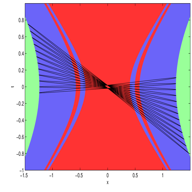
(a)

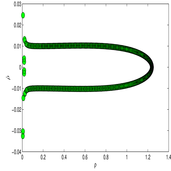
(b)

Figure 1: (color online) (a) The trajectory in the x-t plain. The blue area is the stable area. The red area is an unstable area where only one of the conditions for instability is met. The green area is an unstable area where both conditions of instability are met and the instability is the strongest. (b) The Poincare plot of the motion using $\omega$ as the period of the motion.

We can see that the trajectory crosses the red areas but doesn’t go into the green area where the instability is the strongest. We can also see that in the blue area, the trajectory doesn’t change its direction or crosses itself, however when the trajectory enters the unstable region around the origin, trajectory crosses itself; and when it reaches the green area, it changes its direction. This pattern will be conserved until the trajectory runs off to infinity.
We can also see that the Poincaré plot doesn’t indicate chaotic behavior since the trajectory crosses the $\rho-\dot{\rho}$ plan in a different point every period but there is a distinct pattern to these crossings and for the case of $f=0$, it is also symmetric around $\dot{\rho}=0$.

Other plots we wish to examine are those of the trajectory in each dimension as a function of $\tau$ (fig.2).

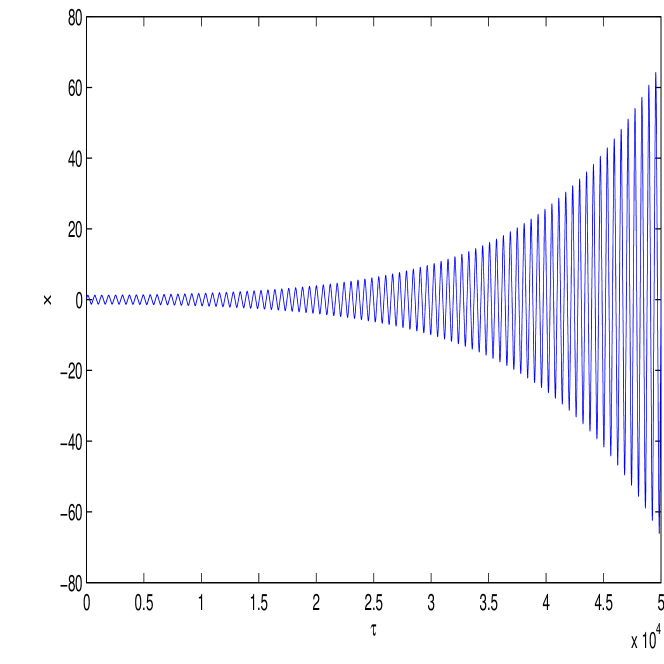
(a)

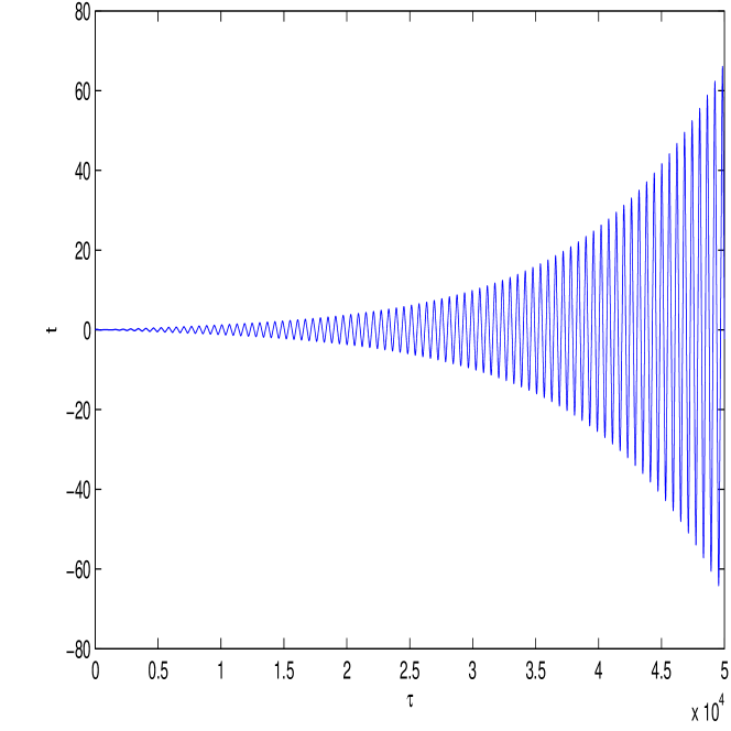
(b)

Figure 2: Both x (a) and t (b) as functions of $\tau$ shows expanding oscillations with a distinct pattern and what seems to be a constant period in $\tau$.

The trajectories on the x-$\tau$ and t-$\tau$ planes have distinct patterns and they do not exhibit chaotic behavior.

We now add a driving force and set $f=0.05$ and examine the results (fig.3).

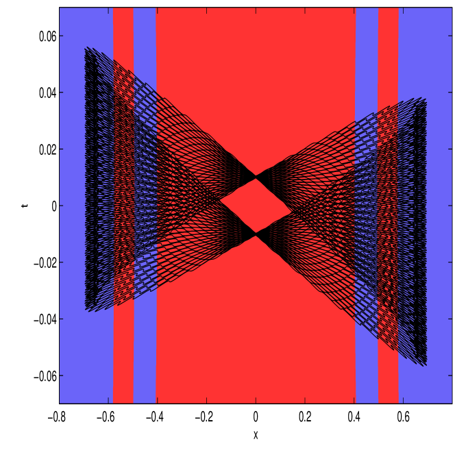
(a)

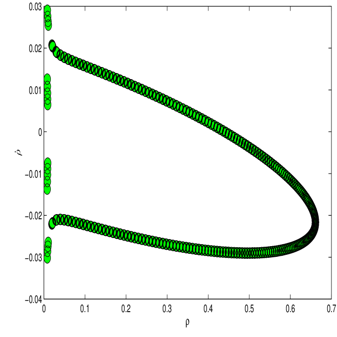
(b)

Figure 3: The motion under the influence of a small driving force, is contained within a small area around the origin and crosses the unstable regions there (a). We can also see that the trajectory crosses the $\rho-\dot{\rho}$ plan in a different point every period but there is a distinct pattern to these crossings (b).

We can see that by adding this small driving force, the trajectory stays around the origin and doesn’t spread. We can also see that the trajectory crosses the unstable red area but doesn’t go into the green area. This motion doesn’t indicate chaotic behavior. The fact that at each period, the crossing of the $\rho-\dot{\rho}$ plane occurs on a different point and never twice at the same point implies unstable behavior, however, there is a distinct pattern spread over a very small area which does not indicate chaotic behavior, although the plot is no longer symmetric around $\dot{\rho}=0$ due to the driving force.

Examining the the trajectory in each dimension as a function of $\tau$ we get the results in (fig.4).

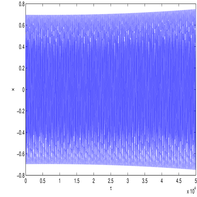
(a)

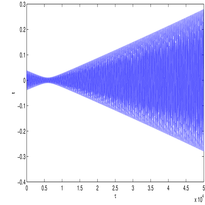
(b)

Figure 4: Both x (a) and t (b) as functions of $\tau$ shows oscillations with a distinct pattern and what seems to be a constant period in $\tau$.

The trajectories of $t$ as a function of $\tau$ snd $x$ as a function of $\tau$ do not imply such behavior as well. We see that there is a distinct pattern of these plots and what seems to be a constant period of the motion.

If we take f=1 (fig.5),

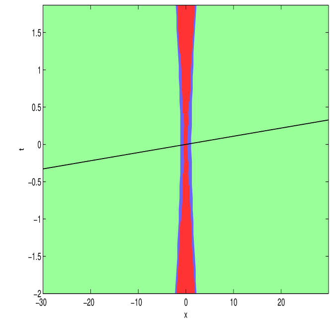
(a)

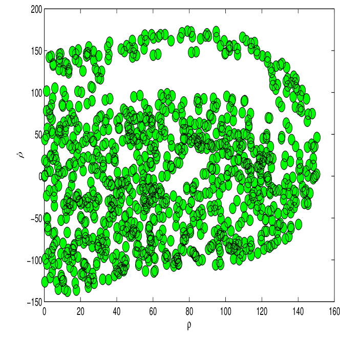
(b)

Figure 5: (a)The trajectory we get from the equations of motion for $E=1$ and $f=1$ over the different regions. (b)The Poincare plot for $E=1$ and $f=1$ using $\omega$ as the period of the motion. Approximatelty $1000$ points are represented in this figure.

we see that the trajectory (fig.5a) oscillates in a wide range of x and goes deep into the green area where the instability is the strongest. The Poincare plot (fig.5b) is scattered randomly with no distinct pattern, suggesting chaotic behavior. We find no regularity in the resulting plots.

If we focus on the trajectory and enlarge it significantly, we will see that there are 2 sets of trajectories (fig.6).

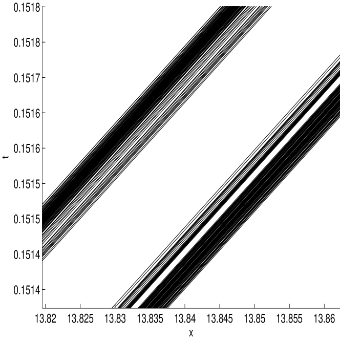
Figure 6: A closer look at the trajectory reveals two distinct subsets

Each contains a group of close-by sub-trajectories - which matches the two potential wells of the Duffing oscillator and it looks like a period doubling which suggests chaotic behavior.

Also, the trajectories of $x$ vs $\tau$ (fig.7a) and $t$ vs $\tau$ (fig.7b) imply such behavior.Both plots indicate chaotic behavior.

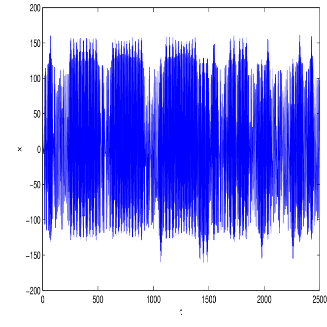
(a)

(b)

Figure 7: Both x (a) and t (b) as functions of $\tau$ shows no distinct pattern or a period in $\tau$.

The value of the driving force that seems to be the boundary between stability and instability for E=1 appear to be f=0.71, i.e., larger values provide clearly unstable behavior, and smaller values, clearly stable. For this choice, we obtain (fig.8) and (fig.9), demonstrating what might be expected of a threshold behavior.

In this case, we obtain (fig.8).

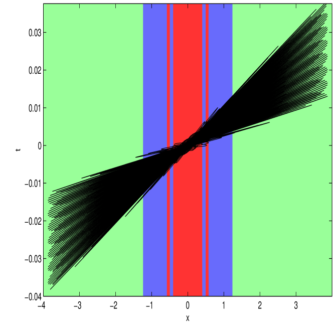
(a)

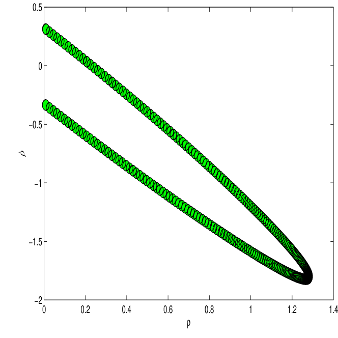
(b)

Figure 8: The trajectory we get from the equations of motion for $E=1$ and $f=0.71$ over the different regions (a) and its Poincare plot using $\omega$ as the period of the motion (b)

We can see that the trajectory (fig.8a) goes into the green areas, but it doesn’t go very deep into it and the Poincare plot (fig.8b) doesn’t suggest chaotic behavior. Although we can still see a pattern, the Poincare plot spreads on a much wider range of values now, which indicates that the pattern is about to break.

Taking a closer look at the trajectory we see the result (fig.9);

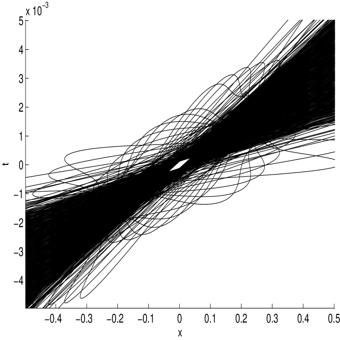
Figure 9: A closer look at the trajectory doesn’t show the pattern that we identified for small values of $f$ or the subsets that we saw for large values of $f$

This image indicates the beginning of chaotic behavior. We can’t see periodic doubling doubling at this level, but the pattern that we saw for a small value of $f$ is already broken.

Also, the trajectories of $x$ vs $\tau$ (fig.10a) and $t$ vs $\tau$ (fig.10b) seems to imply the same.

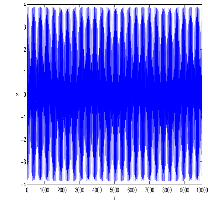
(a)

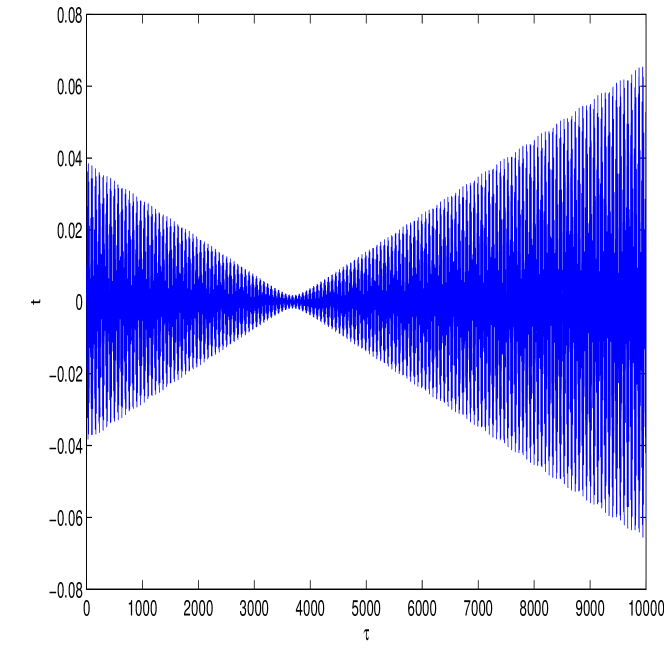
(b)

Figure 10: Both $x$ (a) and $t$ (b) as functions of $\tau$ show some pattern and a period in $\tau$. Both the pattern and the period don’t seem to be very distinct and it appears that they are about to break.

The trajectories don’t seem to be chaotic yet, but it looks as if the pattern is reaching a threshold for chaotic behavior as realized in (fig.5).

VI Conclusions

We have studied a method of determining criteria for stablilty of a relativistic system. First, we performed a conformal transformation on the original relativistic Hamiltonian which was in flat-space coordinates, and embedded it into a curved space. Then, we used the geodesic equation of the curved space in order to obtain a connection form for the seconed derivative in the original flat space and from that, we derived a geodesic deviation eqation that depends only on the flat space coordinates and their derivatives.

Next, we used the criteria that we found and applied it to a two body Hamiltonian in $1+1$ dimensions with a Duffing oscillator relative potential $V(y)$, where $y^{\mu}=y_{1}^{\mu}-y_{2}^{\mu}$, with $y_{1}^{\mu}$ and $y_{2}^{\mu}$ the coordinates of each of the particles, with a driving force. Our results describe the relative motion of the two body system. Since we are working in $1+1$ dimensions the corresponding (spacelike) orbital motion is completely described dynamically by the invariant $\rho=\sqrt{y^{\mu}y_{\mu}}$ and a hyperbolic angle $\beta$ [14] for which the space component is $y=\rho\cosh\beta$ and the time component is $t=\rho\sinh\beta$; our results are given in terms of the variable $x$ defined by Eqs. $(14)$ and $(15)$.

We found unstable regions in the relativitic flat-space and calculated the trajectory for given initial conditions and a different driving forces numerically.

We found two conditions for instability and discovered that there are two different types of instability: the first is when only one of the conditions is met and the second is when both conditions are met. The second type of instability is stronger and if the driving force is strong enough so that the trajectory enters such a region, then chaotic behavior appears to be generated.

We found the threshold driving force value to be $f\approx 0.71$. For this value of $f$, the trajectory enters the region where both conditions of instability are met and chaotic behavior is starting to take place.

References

- [1] E. C. G. Stueckelberg. Remarks on the creation of pairs of particles in the theory of relativity. Helv. Phys. Acta, 14:588–594, 1941.
- [2] L.P. Horwitz and C. Piron. Relativistic dynamics. Helv. Physica Acta, 46:316, 1973.
- [3] Lawrence P Horwitz. Relativistic Quantum Mechanics, Fundamental Theories of Physics 180. Springer, 2015.
- [4] LP Horwitz, RI Arshansky, and AC Elitzur. On the two aspects of time: The distinction and its implications. Foundations of Physics, 18(12):1159–1193, 1988.
- [5] LP Horwitz, WC Schieve, and Constantin Piron. Gibbs ensembles in relativistic classical and quantum mechanics. Annals of Physics, 137(2):306–340, 1981.
- [6] R Arshansky and LP Horwitz. The quantum relativistic two-body bound state. I. the spectrum. Journal of Mathematical Physics, 30(1):66–80, 1989.
- [7] R Arshansky and LP Horwitz. The quantum relativistic two-body bound state. II. the induced representation of sl (2, c). Journal of Mathematical Physicsathematical physics, 30(2):380–392, 1989.
- [8] Lawrence Horwitz, Yossi Ben Zion, Meir Lewkowicz, Marcelo Schiffer, and Jacob Levitan. Geometry of Hamiltonian chaos. Physical Review Letters, 98(23):234301, 2007. Other methods for predicting instability of nonrelativistic systems are discussed as well in this paper; it was found that the method proposed there (GEM) was very effective for a wide range of systems. Criteria for predicting the stability of relativistic dynamical systems of the type considered here have not been previously discussed.
- [9] Martin C Gutzwiller. Chaos in Classical and Quantum Mechanics, volume 1. Springer Science & Business Media, 2013. The notion of geodesic deviation arises as well in general relativity, for example, the discussion in S. Weinberg, "Gravitation and Cosmology: Principles and Applications of the General Theory of Relativity", Wiley, New York (1973).
- [10] Yossi Ben Zion and Lawrence Horwitz. Applications of geometrical criteria for transition to Hamiltonian chaos. Physical Review E, 78(3):036209, 2008.
- [11] RI Arshansky and LP Horwitz. Solutions of the quantum relativistic two-body bound state problem with invariant direct action potentials. Physics Letters A, 128(3):123–128, 1988.
- [12] Avi Gershon and Lawrence Horwitz. Kaluza-Klein theory as a dynamics in a dual geometry. Journal of Mathematical Physics, 50(10):102704, 2009.
- [13] Charles W Misner, Kip S Thorne, and John Archibald Wheeler. Gravitation. Macmillan, 1973.
- [14] WC Schieve and LP Horwitz. Chaos in the classical relativistic mechanics of a damped Duffing-like driven system. Physics Letters A, 156(3):140–146, 1991.