Effects of Degree Correlations in Interdependent Security: Good or Bad?

Abstract

We study the influence of degree correlations or network mixing in interdependent security. We model the interdependence in security among agents using a dependence graph and employ a population game model to capture the interaction among many agents when they are strategic and have various security measures they can choose to defend themselves. The overall network security is measured by what we call the average risk exposure (ARE) from neighbors, which is proportional to the total (expected) number of attacks in the network.

We first show that there exists a unique pure-strategy Nash equilibrium of a population game. Then, we prove that as the agents with larger degrees in the dependence graph see higher risks than those with smaller degrees, the overall network security deteriorates in that the ARE experienced by agents increases and there are more attacks in the network. Finally, using this finding, we demonstrate that the effects of network mixing on ARE depend on the (cost) effectiveness of security measures available to agents; if the security measures are not effective, increasing assortativity of dependence graph results in higher ARE. On the other hand, if the security measures are effective at fending off the damages and losses from attacks, increasing assortativity reduces the ARE experienced by agents.

I Introduction

As many critical engineering systems, such as power grids, become more connected, there is a growing interest in understanding the security of large, complex networks in which security of many comprising agents or subsystems is interdependent. This is dubbed interdependent security (IDS) by Kunreuther and Heal [17]. It arises naturally in many settings, and examples include cybersecurity [7, 14, 25, 26], cyber-physical systems security (e.g., power grids) [8], epidemiology [30, 34], financial networks and systems [4, 9, 10], homeland security [13, 18], and supply chain and transportation system security (e.g., airline security) [12, 16].

The sizes and complexity of these systems as well as the number of participating agents introduce several major challenges to studying their reliability and security. This is especially the case when they contain many individuals, organizations or (sub)systems that can make local security decisions based on locally observable risks. Throughout the manuscript, we refer to these individuals, organizations or systems that make own security decisions simply as agents.

First, in many cases, it is reasonable to assume that the agents are rational or strategic and are only interested in their own objectives with little or no regards for others. Therefore, a study of static settings in which the agents make decisions without taking into account the experienced risks may not be realistic. Second, in IDS settings, the security of individual agents is interdependent, thereby causing the agents’ security decisions to be coupled as a result of externalities produced by security measures they employ. Furthermore, these externalities and the resulting security risks seen by agents depend on the properties of their dependence structure. Third, any attempt to model and study detailed interactions between many strategic agents suffers from the curse of dimensionality. Finally, while there are some popular metrics used in the literature (e.g., global cascade probability), there is a lack of standard metrics on which security experts agree for measuring network- or system-level security.

As mentioned above, the security of the systems in IDS settings depends on many system properties, including the properties of interdependence in security among agents, which we model using a dependence graph. Although the effects of some graph properties (e.g., degree distributions and clustering [11, 19, 20]) have been recently studied in the literature, to the best of our knowledge, the influence of the degree correlations in the dependence graph with strategic agents has not been examined before. The degree correlations, which are also known as assortative mixing, (degree) assortativity or network mixing, refer to the correlations in the degrees of end nodes of edges present in the graph.

It has been shown [28, 29] that engineered networks, e.g., the Internet, tend to be disassortative, whereas social networks are typically assortative. In other words, nodes in engineered systems tend to be connected to other nodes with dissimilar degrees, while those in social networks exhibit a tendency to be neighbors with other nodes with similar degrees. These correlations in the degrees of end nodes in the dependence graph change the security risk experienced by agents from their neighbors based on their own degrees. This is because the security investments chosen by agents with different degrees are likely to vary and some agents are more vulnerable to attacks than others. The goal of our study is to shed some light on how the degree correlations in the dependence graph affect the security investments of strategic agents and, in doing so, the overall system security.

While there have been some numerical studies on the influence of network mixing on the robustness of networks in static settings (e.g., [28, 29]), as we will discuss in Section II, there are two key differences between our study and existing studies: (i) In our study, agents are strategic and can choose how much they wish to invest in security in response to the security risks they experience. (ii) The security measures adopted by an agent (e.g., incoming traffic monitoring, anti-malware utility) produce positive externalities [37] and alter the security risks and threats seen by other agents in the network, thereby influencing their security investments.

It is shown that positive externalities produced by security measures on neighbors often lead to free riding [19, 20, 26]; when some agents invest in security measures, positive externalities they generate curtail the risk experienced by other agents, thus reducing their incentive to protect themselves and invest in security. Consequently, they cause under-investments in security by strategic agents and social inefficiency [39]. For this reason, the presence of externalities in IDS considerably complicates the analysis of the interactions among strategic agents.

Let us illustrate these concepts with the help of the following example.

$\diamond$ Spread of malware via emails: When a user’s device is infected by malware, it can scan the user’s emails or the hard disk drive of the infected machine and send the user’s personal or other confidential information to criminals interested in stealing, for instance, the user’s identity (ID) or trade secrets. Moreover, the malware can browse the user’s address book and either forward it to attackers or send out bogus emails, i.e., email spoofing, with a link or an attachment to those on the contact list. When a recipient clicks on the link or opens the attachment, it too becomes infected.

In order to reduce the risks or threats from malware, users can install an anti-malware utility on their devices. When a user adopts an anti-malware tool, not only does it reduce its own risk, but it also lessens the risk to those on its address book for the reason stated above, in doing so protecting its friends to some degree. Therefore, it produces positive externalities for others [36, 37]. Interestingly, these positive externalities diminish the benefits of installing anti-malware utilities for others, thus introducing negative network effects for them.

I-A Summary and main contributions

For mathematical tractability, we employ a population game [33] to model the interactions among agents. This model is a generalization of the model used in our previous studies that considered neutral dependence graphs [19, 20]; we assume a continuous action space, where an action represents the security investment chosen by an agent with an understanding that the agent selects the best combination of security measures subject to the budget constraint.

In order to measure the global network security and the local security experienced by individual agents, which is then utilized for choosing security investments, we adopt what we call the average risk exposure (ARE) from neighbors. While other global metrics, such as the probability of cascading failures/infections, have been adopted by existing studies, including our previous study [20], we argue that the ARE is a more natural and meaningful metric for our purpose for the following reasons.

Since the agents can base their decisions only on local information or risks they can observe and assess, we need to model the local security risks they experience. First, we will show that the ARE captures the average security risks agents of varying degrees perceive from a neighbor, which allow them to approximate their total security risks from all neighbors. Second, the agents are unlikely to have access to the value of a commonly adopted global metric (e.g., cascade probability) as they lack global information, including network topology and the security decisions of other agents. This makes such global metrics unsuitable as information on which the agents can act. In contrast, the ARE also serves as a global security metric because it is proportional to the total (expected) number of attacks in the network. For this reason, it provides us with a consistent metric for (a) measuring the global security and (b) capturing the local security information on which agents act, and enables us to compare the overall network security as we vary the properties of dependence graph.

Our main contributions can be summarized as follows:

S1. We show that there exists a unique (pure-strategy) Nash equilibrium (NE) of a population game under a mild technical condition. Then, we examine how the assortativity of dependence graph changes the ARE at the unique NE as agents with varying degrees experience different risks from their neighbors due to degree correlations. In particular, we prove that when the agents with larger degrees in the dependence graph see higher risks than those with smaller degrees, the overall network security deteriorates in that the ARE experienced by agents increases and there are more attacks in the network.

S2. Making use of this finding, we demonstrate that the effects of network mixing on ARE depend on the cost effectiveness of security measures available to agents; if the security measures are not effective, increasing assortativity of dependence graph results in higher ARE. On the other hand, if the security measures are effective at lowering the damages and losses from attacks, increasing assortativity reduces the ARE experienced by agents.

S3. Using numerical studies, we examine how the cost effectiveness of security measures and the sensitivity of ARE to the vulnerability of agents to attacks shapes the influence of assortativity. Numerical results suggest that as security measures improve and become more effective at fending off attacks, the assortativity of dependence graph has greater effects on network security. Similarly, when ARE is more sensitive to agents’ vulnerability to attacks, assortativity has stronger impact on equilibrium ARE.

As summarized in the following section, existing studies demonstrated that the assortativity of a network can significantly affect its robustness and resilience, e.g., [29, 38, 39]. Thus, understanding the effects of dependence graph properties is important to (i) predicting the overall network- or system-level security and (ii) devising sound policies.

While we admit that our analysis is carried out using a simplified model, to the best our knowledge, our work here and in [19, 20, 21] is the first (analytical) study of how the network security is shaped by the properties of dependence graph that governs the interdependence in security among strategic agents. Unlike our previous studies that assumed neutral dependence graphs, however, the focus of the current study is the impact of degree correlations in the dependence graph on network security. As summarized earlier, incorporating the strategic nature of agents leads to somewhat unexpected and interesting observation that the net influence of degree correlations is also determined by the effectiveness of available security measures.

We believe that the qualitative nature of our findings provides valuable insights into the behavior of strategic agents in IDS settings, which we hope would be helpful in (i) understanding the pitfalls in studying the security of complex systems and (ii) designing better security policies and regulations. Finally, we emphasize that our goal is to understand the effects of heterogeneous security risks experienced by agents based on their degrees (due to degree correlations) on network security, as opposed to accurate modeling of assortativity observed in real networks. Thus, it is not our intent to develop a more accurate model of dependence graphs with degree correlations.

The remainder of the paper is organized as follows: We provide a short survey of closely related literature in Section II. Section III describes the population game model we adopt for our analysis, and Section IV introduces the security metric we employ for comparing network security and explains how we model the effects of degree correlations. Section V introduces some preliminary results we need for our main findings reported in Section VI. Numerical results are provided in Section VIII. We conclude in Section IX.

II Related literature

There are existing studies on IDS, many of which employ a game theoretic approach to model the strategic nature of agents (e.g., [14, 16, 17]). We refer an interested reader to a survey paper by Laszka et al. [27] and references therein for a succinct discussion of these and other related studies. In addition, many researchers investigated the existence of assortativity in many different types of networks, e.g., [2, 29, 31, 38]. Here, we only focus on studies that examined the effects of assortativity in epidemics or security-related settings and summarize their main findings.

In [28, 29], Newman studied network mixing in different types of networks, including biological networks, engineered networks, and social networks. He first showed that while social networks in general exhibit assortativity, both engineered and biological networks tend to be disassortative. He then investigated how assortativity affects the phase transition in the emergence of a giant component in random graphs as the average degree of nodes increases.

His findings revealed that stronger assortativity makes it easier for a giant component to appear, but at the same time, the size of the giant component tends to be smaller. Furthermore, breaking up the giant component by removing a subset of nodes with the highest degrees becomes more difficult when the network is assortative; the numerical results suggest that the number of nodes that must be removed from the network to split up the giant component in an assortative network can be an order of magnitude larger than that of a disassortative network.

He argued that these findings have following important implications. First, preventing an outbreak of a disease via vaccination of high-degree individuals can be problematic because social networks exhibit assortativity and the cluster of high-degree nodes could serve as a reservoir of disease. However, for the same reason, an epidemic will likely be limited to a smaller portion of population if an outbreak does occur. On the other hand, improving the resilience of engineered networks, such as the Internet, which show disassortativity becomes more challenging as disassortative networks are more susceptible to coordinated attacks that target high-degree nodes in the networks.

In [5, 6], Bogu$\tilde{\rm n}\acute{\rm a}$ et al. studied the (existence) of epidemic threshold in scale-free networks, using the popular susceptible-infected-susceptible model. The key finding of the study was that the degree correlations do not significantly affect the existence of epidemic threshold as long as the degree correlations are limited to immediate neighbors. Instead, the (lack of) the existence of threshold is shaped by the divergence of the second moment of node degrees when the power law exponent lies in the interval (2, 3].

Another related study by Zhou et al. [40] investigated the influence of assortativity on the robustness of interdependent networks with the help of independent failure model, using both Erd$\ddot{\rm o}$s-R$\acute{\rm e}$nyi networks and scale-free networks. Their main finding suggests that increasing assortativity leads to deteriorating robustness of interdependent network; as a network becomes more assortative, the initial number of nodes that need to be removed in order to break up the giant component in the network drops. This indicates that it is easier to break up the giant component in an interdependent network by eliminating randomly chosen nodes.

In a more concrete cybersecurity application, Yen and Reiter [38] studied how the assortativity of botnets influences the performance of takedown strategies. They first demonstrated that botnets exhibit high assortativity and attributed this in part to the working of botnets. Secondly, they showed that some of well studied takedown strategies, in particular uniform takedown and degree-based takedown strategies, are far less effective as the botnets become more assortative. This finding suggests that previous studies carried out with neutral botnets may be inaccurate and incorrectly portray a more optimistic picture. Finally, they also considered other alternative takedown strategies that take into account clustering coefficients and closeness centrality and showed that a similar trend continues.

We note that these studies do not take into consideration the strategic nature of individual agents that can make their own security decisions, which is natural in many settings of interest. Our study considers strategic agents that determine their security investments in response to the security risks they observe. In addition, rather than focusing on giant components in networks and possible cascades of infection, we analyze the (local) network security experienced by individual agents as a result of their security decisions at equilibria.

We studied related problems in [19, 20, 21] under neutral dependence graphs. In [21], we investigated (i) how we could improve the overall (network) security by internalizing the externalities produced by the security measures adopted by agents and (ii) how the sensitivity of network security to agents’ security investments influences the penalties or taxes that need to be imposed on the agents to internalize externalities. Moreover, we showed [19, 21] that as the security of agents gets more interdependent in that their degrees in the dependence graph become larger (with respect to the usual stochastic order [35]), the security experienced by agents whose degrees remain fixed improves in that the number of attacks they suffer goes down. Thus, this finding tells us, to some extent, how the degree distribution in the dependence graph affects the network security.

In [20], we considered a simple model where agents can choose from three possible actions: i) invest in security, ii) purchase security insurance to transfer (some of) risks, and iii) take no actions. Using this model, we carried out numerical studies that examined how the degree distribution of dependence graph affects the cascade probability. Our study demonstrated that as the interdependence in security rises, so does the probability of cascade. Moreover, we derived an upper bound on the price of anarchy, i.e., the ratio of the social cost at the Nash equilibrium to that of the social optimum, which is a linear function of the average node degree.

We point out that none of the above studies, including our own studies, investigated the role of network mixing in IDS settings with strategic agents and no analytical findings have been reported. A key difference between our study in [19, 21] and the current study is the following: our previous study focused on how varying degree distributions influence the network security in a neutral dependence graph. The current study, on the other hand, considers a fixed degree distribution and examines how differing security risks seen by agents based on their own degrees (due to degree correlations), shape the resulting network security. Some of our preliminary results have been reported in [22]. It, however, employs a simpler, hence more restrictive model to facilitate the analysis.

III Model

We capture the interdependence in security among the agents using an undirected graph, which we call the dependence graph. A node or vertex in the graph corresponds to an agent (e.g., an individual or organization), and an undirected edge between nodes $n_{1}$ and $n_{2}$ implies interdependence of their security. We interpret an undirected edge as two directed edges pointing in the opposite directions with an understanding that a directed edge from node $n_{1}$ to node $n_{2}$ indicates that the security of node $n_{1}$ affects that of node $n_{2}$ in the manner we explain shortly. When there is an edge between two nodes, we say that they are immediate or one-hop neighbors or, simply, neighbors when it is clear.

We model the interaction among agents as a noncooperative game, in which players are the agents. This is reasonable because, in many cases, it may be difficult for agents to cooperate with each other and take coordinated countermeasures to attacks. In addition, even if they could coordinate their actions, they would be unlikely to do so when there are no clear incentives for coordination.

We are interested in scenarios where the number of agents is large. Unfortunately, modeling detailed microscale interactions among many agents in a large network and analyzing ensuing games is difficult; the number of possible strategy profiles typically increases exponentially with the number of players and finding the NEs of noncooperative games is often challenging even with a moderate number of players.

The notation we adopt throughout the paper is listed in Table I.

$C({\bf x},d,a,{\bf s})$	Cost of an agent with degree $d$ playing action $a$ at
	social state ${\bf x}$
${\mathcal{D}}$	Set of agent degrees or populations
	(${\mathcal{D}}=\{1,2,\ldots,D_{\max}\}$)
$D_{\max}$	Maximum degree among agents or the number of
	populations, i.e., $D_{\max}=|{\mathcal{D}}|$
${\mathcal{I}}$	(Pure) action space (${\mathcal{I}}=[I_{\min},I_{\max}]$)
$I^{{\rm opt}}(r)$	Optimal security investment of an agent facing $r$
	expected attacks
$L$	Average loss from a single infection
${\mathcal{P}}_{{\mathcal{I}}}$	Set of probability distributions over ${\mathcal{I}}$
${\mathcal{X}}$	Cartesian product ${\mathcal{P}}_{{\mathcal{I}}}^{D_{\max}}$
$d_{{\rm avg}}$ or $d_{{\rm avg}}({\bf s})$	Average or mean degree of agents
	($d_{{\rm avg}}({\bf s})=\sum_{d\in{\mathcal{D}}}d\cdot f_{d}({\bf s})$)
$e_{{\rm avg}}({\bf x},{\bf s})$	Average risk exposure at social state ${\bf x}$
$e_{d}({\bf x},{\bf s})$	Risk exposure of pop. $d$ at social state ${\bf x}$
$f_{d}$ or $f_{d}({\bf s})$	Fraction of agents with degree $d$
	($f_{d}({\bf s})=s_{d}/\sum_{d^{\prime}\in{\mathcal{D}}}s_{d^{\prime}}$)
${\bf g}$	Mixing vector (${\bf g}=(g_{d};\ d\in{\mathcal{D}})$)
$p(a)$	Infection prob. of an agent investing $a$ in security
$p^{\star}(r)$	Infection prob. of an agent facing $r$ expected attacks
	and investing $I^{{\rm opt}}(r)$ in security
	($p^{\star}(r)=p(I^{{\rm opt}}(r))$)
$p_{d,{\rm avg}}({\bf x})$	Average infection prob. of population $d$ at social
	state ${\bf x}$
${\bf s}$	Pop. size vector (${\bf s}=(s_{d};\ d\in{\mathcal{D}})$)
$s_{d}$	Size of pop. $d\in{\mathcal{D}}$
$w_{d}$ or $w_{d}({\bf s})$	Weighted fraction of agents with degree $d$
	($w_{d}({\bf s})=\frac{d\cdot s_{d}}{\sum_{d^{\prime}\in{\mathcal{D}}}d^{\prime}\cdot s_{d^{\prime}}}=\frac{d\cdot f_{d}({\bf s})}{d_{{\rm avg}}({\bf s})}$ )
${\bf x}_{d}$	Pop. state of pop. $d$
${\bf x}$	Social state (${\bf x}=({\bf x}_{d};\ d\in{\mathcal{D}})$)
$\beta_{IA}$	Prob. of indirect attack on a neighbor by an infected
	agent
$\tau_{A}$	Prob. that an agent experiences a direct attack

TABLE I: Notation (pop. $=$ population, prob. $=$ probability).

III-A Population game model

For analytical tractability, we adopt a population game with a continuous action space to model the interaction among the agents [33]. As stated earlier, the (local) network security is captured using ARE from neighbors. As we explain in Section IV-A, the ARE is proportional to the total (expected) number of attacks that propagate from the victims of successful attacks to their neighbors in the network and can be viewed as a measure of global network security.

We assume that the maximum degree among all agents in the dependence graph is $D_{\max}<\infty$. For each $d\in\{1,2,\ldots,D_{\max}\}=:{\mathcal{D}}$, population $d$ consists of all agents with common degree $d$. Let $s_{d}$ denote the size or mass of population $d$, and the population size vector ${\bf s}:=\big{(}s_{d};\ d\in{\cal D}\big{)}$ tells us the sizes of populations with varying degrees.

We find it convenient to define ${\bf f}({\bf s}):=(f_{d}({\bf s});\ d\in{\mathcal{D}})$, where $f_{d}({\bf s})=s_{d}/\sum_{d^{\prime}\in{\mathcal{D}}}s_{d^{\prime}}$ is the fraction of agents with degree $d$ in the dependence graph. Given a population size vector ${\bf s}$, we denote the average degree of agents by $d_{{\rm avg}}({\bf s}):=\sum_{d\in{\mathcal{D}}}d\cdot f_{d}({\bf s})$. When there is no confusion, we simply denote ${\bf f}({\bf s})$ and $d_{{\rm avg}}({\bf s})$ by ${\bf f}$ and $d_{{\rm avg}}$, respectively.

$\bullet$ Population state and social state – All agents have the same action space ${\mathcal{I}}=[I_{\min},I_{\max}]\subset{\rm I\kern-2.5ptR}_{+}:=[0,\infty)$, where $I_{\min}<I_{\max}<\infty$. A (pure) action taken by an agent represents the security investment made by the agent. We denote the set of probability distributions over ${\mathcal{I}}$ by ${\cal P}_{\mathcal{I}}$.

The population state of population $d$ is given by ${\bf x}_{d}\in{\cal P}_{\mathcal{I}}$. In other words, given any (Borel) subset ${\cal S}\subseteq{\mathcal{I}}$, ${\bf x}_{d}({\cal S})$ tells us the fraction of population $d$ whose security investment lies in ${\cal S}$. The social state, denoted by ${\bf x}=({\bf x}_{d};\ d\in{\mathcal{D}})\in{\mathcal{X}}:={\cal P}_{\mathcal{I}}^{D_{\max}}$, specifies the actions chosen by all agents.

$\bullet$ Two types of attacks – In order to understand how the degree correlations of dependence graph affect the security investments of the agents and overall network security, we model two different types of attacks agents suffer from – direct and indirect attacks. While the first type of attacks is independent of the dependence graph, the latter depends on it, allowing us to capture the externalities produced by agents’ security choices.

a) Direct attacks: We assume that malicious attackers launch attacks on the agents, which we call direct attacks. While our model can be easily modified to handle a scenario in which an agent can suffer more than one direct attack from different attackers by modifying the cost function, here we assume that an agent experiences at most one direct attack and the probability of bearing a direct attack is $\tau_{A}$, independently of other agents.

When an agent experiences a direct attack, its cost depends on its security investment; when an agent adopts action $a\in{\mathcal{I}}$, it is infected with probability $p(a)\in[0,1]$. Also, each time an agent is infected, it incurs on the average a cost of $L$. Hence, the expected cost or loss of an agent from a single attack is $L(a):=L\cdot p(a)$ when investing $a$ in security.

It is shown [3] that, under some technical assumptions, the security breach probability or probability of loss is a log-convex (hence, strictly convex) decreasing function of the investments. Based on this finding, we introduce the following assumption on the infection probability $p(a)$, $a\in{\mathcal{I}}$.

Assumption 1

The infection probability $p:{\mathcal{I}}\to[0,1]$ is continuous, decreasing and strictly convex. Moreover, it is continuously differentiable on ${\rm int}({\mathcal{I}})=(I_{\min},I_{\max})$.

b) Indirect attacks: Besides the direct attacks by the attackers, an agent may also experience indirect attacks from its neighbors that have sustained successful attacks and are infected. We assume that an infected agent will unwittingly participate in indirect attacks on its neighbors, each of which is attacked with probability $\beta_{IA}\in(0,1]$ independently of each other. When an agent investing $a$ in security suffers an indirect attack, it is infected with the same infection probability $p(a)$.

We call $\beta_{IA}$ indirect attack probability (IAP). It affects the local spreading behavior. Unfortunately, the dynamics of infection propagation depend on the details of underlying dependence graph, which are difficult to obtain or model faithfully. In order to skirt this difficulty, instead of attempting to model the detailed dynamics of infection transmissions between agents, we abstract out the security risks seen by the agents using the expected number of attacks an agent sees from its neighbors. However, to capture the effects of network mixing, we allow agents of varying degrees to experience different risks from their neighbors as explained below and in Section IV.

$\bullet$ Cost function – The cost function of the game is determined by a function $C:{\mathcal{X}}\times{\mathcal{D}}\times{\mathcal{I}}\times{\rm I\kern-2.5ptR}_{+}^{D_{\max}}\to{\rm I\kern-2.5ptR}$. The interpretation is that, when the population size vector is ${\bf s}$ and the social state is ${\bf x}$, the cost of an agent with degree $d$ (hence, from population $d$) playing action $a\in{\mathcal{I}}$ (thus, investing $a$ in security) is equal to $C({\bf x},d,a,{\bf s})$. As we will show below, in addition to the cost of security investments, our cost function also reflects the (expected) losses from attacks.

Given a social state ${\bf x}\in{\mathcal{X}}$, let $e_{d}({\bf x},{\bf s})$ denote the average number of indirect attacks an agent with degree $d\in{\mathcal{D}}$ sees from a single neighbor. Hence, the average number of indirect attacks experienced by agents of degree $d$ would be $d\cdot e_{d}({\bf x},{\bf s})$. One natural metric for the security risk seen by agents is the number of attacks they expect to see. Hence, $e_{d}({\bf x},{\bf s})$ captures the security risk per neighbor observed by agents of degree $d$. We call $e_{d}({\bf x},{\bf s})$ the risk exposure (RE) for population $d$ at social state ${\bf x}$. Since we are interested in understanding how network mixing affects the agents’ security investments, it is necessary to allow the RE to vary from one population to another, i.e., $e_{d}({\bf x},{\bf s})$ and $e_{d^{\prime}}({\bf x},{\bf s})$ can differ if $d\neq d^{\prime}$.

Before we proceed, let us comment on the key difference between the current model and that of our earlier work [21], which only considers neutral dependence graphs with no degree correlations. When the underlying dependence graph is neutral, the degree distribution of neighbors does not depend on the degree of the agent under consideration and the risk exposure is identical for populations, i.e., $e_{d}({\bf x},{\bf s})=e_{d^{\prime}}({\bf x},{\bf s})$ for all $d,d^{\prime}\in{\mathcal{D}}$. As a result, both the model and the analysis become much simpler.

We assume that the costs of an agent due to multiple infections are additive. Hence, the expected cost of an agent with degree $d$ from indirect attacks is proportional to its degree and RE $e_{d}({\bf x},{\bf s})$. The additivity of costs is reasonable in many scenarios, including the earlier example of malware propagation; each time a user is infected by different malware (e.g., ransomware) or its ID is stolen, the user will need to spend time and incur expenses to deal with the problem. Similarly, every time a corporate network is breached, besides any financial losses or legal expenses, the network operator will need to assess the damages and take corrective measures.

Based on this assumption, we adopt the following cost function for our population game: for a given social state ${\bf x}\in{\mathcal{X}}$, the cost of an agent with degree $d$ investing $a$ in security is equal to

$$C({\bf x},d,a,{\bf s}) = \left(\tau_{A}+d\cdot e_{d}({\bf x},{\bf s})\right)L(a)+a.$$ (1)

Note that $\tau_{A}+d\cdot e_{d}({\bf x},{\bf s})$ is the total number of both direct and indirect attacks an agent of degree $d$ expects. Hence, the first term on the right-hand side of (1) is the total expected loss due to infections.

From now on, we take the viewpoint that the agents use their expected number of attacks given by $\tau_{A}+d\cdot e_{d}({\bf x},{\bf s})$ as their perceived security risks at social state ${\bf x}$. Based on these observed risks, they decide their security investments to minimize their cost given in (1).

$\bullet$ Nash equilibria – We focus on the NEs of population games as an approximation to agents’ behavior in practice. For every $d\in{\mathcal{D}}$, define a mapping ${\mathcal{I}}^{{\rm opt}}_{d}:{\mathcal{X}}\to\mathcal{B}({\mathcal{I}})$, where $\mathcal{B}({\mathcal{I}})$ is the set of (Borel) subsets of ${\mathcal{I}}$ and

$${\mathcal{I}}^{{\rm opt}}_{d}({\bf x}):=\left\{a\in{\mathcal{I}}\ \big{|}\ C({\bf x},d,a,{\bf s})=\inf_{a^{\prime}\in{\mathcal{I}}}C({\bf x},d,a^{\prime},{\bf s})\right\}.$$

Definition 1

A social state ${\bf x}^{\star}$ is an NE if ${\bf x}^{\star}_{d}({\mathcal{I}}^{{\rm opt}}_{d}({\bf x}^{\star}))=1$ for all $d\in{\mathcal{D}}$.

Clearly, our model does not require that all agents from a population adopt the same action in general. However, we are often interested in cases in which the social state is degenerate, i.e., all agents with the same degree adopt the same action. In this case, we denote the action chosen by population $d\in{\mathcal{D}}$ by $a_{d}$, and refer to ${\bf a}:=(a_{d};\ d\in{\mathcal{D}})\in{\mathcal{I}}^{D_{\max}}$ as a pure strategy profile.

With a little abuse of notation, we denote the RE of population $d\in{\mathcal{D}}$ when a pure strategy profile ${\bf a}$ is employed by $e_{d}({\bf a},{\bf s})$.

Definition 2

A pure strategy profile ${\bf a}^{\star}\in{\mathcal{I}}^{D_{\max}}$ is said to be a pure-strategy NE if, for all $d\in{\mathcal{D}}$,

$$a^{\star}_{d}\in\arg\min_{a\in{\mathcal{I}}}\big{(}(\tau_{A}+d\cdot e_{d}({\bf a}^{\star},{\bf s}))L(a)+a\big{)}.$$

In other words, every agent in a population adopts the same best response.

IV Average risk exposure and the effects of network mixing

In this section, we first define the security metric we adopt to measure the (global) network security, namely ARE, and describe how we estimate it. Then, we lay out how we model the the influence of degree correlations on the average security risks experienced by agents of varying degrees (measured by the expected number of attacks) via the REs $e_{d}({\bf x},{\bf s})$, $d\in{\mathcal{D}}$.

IV-A Average risk exposure

As mentioned in Section I, we use a metric we call ARE to measure and compare the network security as we study the impact of degree correlations. The ARE is defined to be the (expected) total number of indirect attacks experienced by all agents divided by the number of directed edges in the dependence graph. Since $e_{d}({\bf x},{\bf s})$ is the number of indirect attacks an agent of degree $d$ expects from a single neighbor at social state ${\bf x}$, its expected total number of indirect attacks is $d\cdot e_{d}({\bf x},{\bf s})$. Therefore, the expected total number of indirect attacks in the network is equal to $\sum_{d\in{\mathcal{D}}}\left(s_{d}\times d\cdot e_{d}({\bf x},{\bf s})\right)$, and the ARE is given by

$$e_{{\rm avg}}({\bf x},{\bf s}) = \frac{\sum_{d\in{\mathcal{D}}}s_{d}\cdot d\cdot e_{d}({\bf x},{\bf s})}{\sum_{d\in{\mathcal{D}}}s_{d}\cdot d}$$ (2)

$$= \sum_{d\in{\mathcal{D}}}w_{d}({\bf s})\cdot e_{d}({\bf x},{\bf s}),$$ (3)

where $w_{d}({\bf s}):=d\cdot f_{d}({\bf s})/d_{{\rm avg}}({\bf s})$, $d\in{\mathcal{D}}$.

Since it is by definition proportional to the expected total number of indirect attacks in the network (for fixed degrees in the network), the ARE can be considered a global metric for network security which measures the aggregate security risks to all agents in the form of attacks from neighbors. In the rest of the paper, we take this viewpoint and study how network mixing influences the network security measured by ARE.

While the definition of ARE is simple and intuitive, it does not provide a means of computing ARE unless we already know the REs $e_{d}({\bf x},{\bf s})$ for all populations. Therefore, we need a way to estimate it. Unfortunately, computing the ARE exactly starting with its definition suffers from several major technical difficulties; it depends on the detailed properties of both the dependence graph and the dynamics of infection propagation among agents. Modeling these accurately is difficult, if possible at all. More importantly, such detailed models in general do not yield to mathematical analysis. For these reasons, we seek to approximate ARE.

IV-A1 Approximation of ARE

In order to approximate the ARE (and the REs), we base our model on the following observation: all indirect attacks begin with the first-hop indirect attacks on the immediate neighbors by the victims of successful direct attacks. Thus, it is reasonable to assume that the total number of indirect attacks in the network increases with the number of the first-hop indirect attacks, each of which can initiate a chain of indirect attacks thereafter.

Let

$$p_{d,{\rm avg}}({\bf x}):=\int_{{\mathcal{I}}}p(a)\ {\bf x}_{d}(da)$$

be the probability that a randomly selected agent of degree $d$ will suffer an infection from a single attack at social state ${\bf x}$. The expected number of agents with degree $d$ which will fall victims to direct attacks is $\tau_{A}\cdot s_{d}\cdot p_{d,{\rm avg}}({\bf x})$, and each infected agent of degree $d$ will attempt to transmit the infection to each of its $d$ neighbors with IAP $\beta_{IA}$. Thus, the expected total number of first-hop indirect attacks by the victims infected by direct attacks is equal to $\tau_{A}\cdot\beta_{IA}\ \sum_{d\in{\cal D}}\left(d\cdot s_{d}\cdot p_{d,{\rm avg}}({\bf x})\right)$.

Based on this argument, we approximate the ARE as a strictly increasing function of $\tau_{A}\cdot\beta_{IA}\ \sum_{d\in{\mathcal{D}}}(d\cdot s_{d}\cdot p_{d,{\rm avg}}({\bf x}))$. But, we first normalize it by the total population size and work with the expected number of first-hop indirect attacks per agent, i.e., $\tau_{A}\cdot\beta_{IA}\ \sum_{d\in{\cal D}}\left(d\cdot s_{d}\cdot p_{d,{\rm avg}}({\bf x})\right)/\sum_{d\in{\mathcal{D}}}s_{d}=\tau_{A}\cdot\beta_{IA}\ \sum_{d\in{\cal D}}\left(d\cdot f_{d}({\bf s})\cdot p_{d,{\rm avg}}({\bf x})\right)$, where the equality follows from the definition of ${\bf f}({\bf s})$. In summary, we estimate the ARE using

$$e_{{\rm avg}}({\bf x},{\bf s}) = \Theta\left(\sum_{d\in{\mathcal{D}}}d\ f_{d}({\bf s})\ p_{d,{\rm avg}}({\bf x})\right)$$ (4)

for some strictly increasing function $\Theta:{\rm I\kern-2.5ptR}_{+}\to{\rm I\kern-2.5ptR}_{+}$, which we assume factors in both $\tau_{A}$ and $\beta_{IA}$. A simple example of function $\Theta$ is a linear function, i.e.,

$$e_{{\rm avg}}({\bf x},{\bf s}) = K\sum_{d\in{\mathcal{D}}}d\ f_{d}({\bf s})\ p_{d,{\rm avg}}({\bf x})$$ (5)

for some $K>0$. The exact form of the function $\Theta$ will depend on many factors, including the detailed dynamics of infection propagation, direct attack probability $\tau_{A}$, IAP $\beta_{IA}$, and the timeliness of deployed remedies (e.g., security patches) to stop the spread of infection.

We impose the following assumption on the function $\Theta$.

Assumption 2

The function $\Theta:{\rm I\kern-2.5ptR}_{+}\to{\rm I\kern-2.5ptR}_{+}$ is continuous and strictly increasing. Furthermore, it is continuously differentiable over ${\rm I\kern-2.5ptR}_{++}:=(0,\infty)$.

The first part of the assumption is natural as argued above. While the latter part (i.e., continuous differentiability) is introduced for convenience to facilitate our analysis, we feel that it is reasonable; recall that the ARE is proportional to the expected total number of indirect attacks in the network, and multi-hop indirect attacks can be viewed as offsprings of one-hop indirect attacks, starting with the victims of direct attacks. For this reason, in practice, we expect the average security risk measured by ARE to be a ‘smooth’ function of the expected number of one-hop indirect attacks.

IV-A2 Alternate expression of ARE

Before we proceed, let us provide an alternate expression of ARE, which helps us highlight two distinct sources that influence the ARE and isolate the one of interest to us. To this end, let us define a mapping $\Phi:{\rm I\kern-2.5ptR}_{+}^{D_{\max}}\times{\rm I\kern-2.5ptR}_{+}\to{\rm I\kern-2.5ptR}_{+}$ with $\Phi({\bf s},r)=\Theta(d_{{\rm avg}}({\bf s})\ r)$. From the definition of ${\bf w}({\bf s})$, we have the following equality.

$$\sum_{d\in{\mathcal{D}}}d\ f_{d}({\bf s})\ p_{d,{\rm avg}}({\bf x}) = d_{{\rm avg}}({\bf s})\sum_{d\in{\mathcal{D}}}w_{d}({\bf s})\ p_{d,{\rm avg}}({\bf x})$$

As explained in [20, 21], $\sum_{d\in{\mathcal{D}}}w_{d}({\bf s})\ p_{d,{\rm avg}}({\bf x})$ is the probability that an end node of a randomly selected edge in the dependence graph is vulnerable to an attack, i.e., it becomes infected when attacked, at social state ${\bf x}$. Therefore, it captures on the average how vulnerable neighboring agents are to indirect attacks and, hence, serves as an indicator of how easily an infection might transmit from one agent to another.

Using the definition of the mapping $\Phi$, the ARE can be rewritten as

$$e_{{\rm avg}}({\bf x},{\bf s}) = \Theta\left(d_{{\rm avg}}({\bf s})\sum_{d\in{\mathcal{D}}}w_{d}({\bf s})\ p_{d,{\rm avg}}({\bf x})\right)$$

$$= \Phi\left({\bf s},\sum_{d\in{\mathcal{D}}}w_{d}({\bf s})\ p_{d,{\rm avg}}({\bf x})\right).$$

From (IV-A2), it is obvious that the ARE depends on two measures that capture the ease with which an infection can spread through the network: (a) the average degree of agents, $d_{{\rm avg}}({\bf s})$, indicates on the average how many other agents an infected agent could potentially infect, and (b) $\sum_{d\in{\mathcal{D}}}w_{d}({\bf s})\ p_{d,{\rm avg}}({\bf x})$ tells us how vulnerable neighboring agents are in general.

The first argument of $\Phi$ depends only on the dependence graph and is beyond the control of agents. Moreover, in our study, we assume that the population sizes ${\bf s}$, hence the average degree $d_{{\rm avg}}({\bf s})$, are fixed and study the influence of degree correlations. On the other hand, the second argument is a function of the social state ${\bf x}$ chosen by agents. Thus, it incorporates the effects of degree correlations that induce heterogeneous REs seen by agents of varying degrees and, as a result, alter the equilibrium ARE (and REs) by affecting their security investments.

IV-B The effects of network mixing

The expression in (2) tells us how the REs shape the ARE. Another way of putting this is that, once the agents choose the social state ${\bf x}$ and the REs are fixed for all populations, we can compute the ARE and then infer the relations between the ARE $e_{{\rm avg}}({\bf x},{\bf s})$ and individual REs $e_{d}({\bf x},{\bf s})$, $d\in{\mathcal{D}}$. These relations reveal how the underlying degree correlations bias the REs at the social state ${\bf x}$ (relative to a neutral dependence graph under which $e_{d}({\bf x},{\bf s})=e_{{\rm avg}}({\bf x},{\bf s})$ for all $d\in{\mathcal{D}}$ and all ${\bf x}\in{\mathcal{X}}$). Therefore, they summarize the net effects of degree correlations on security risks experienced by agents based on their degrees.

In this paper, we assume that these relations are approximately linear. In other words, for every $d\in{\mathcal{D}}$, there exists some $g_{d}>0$ such that $e_{d}({\bf x},{\bf s})=g_{d}\cdot e_{{\rm avg}}({\bf x},{\bf s})$ for all ${\bf x}\in{\mathcal{X}}$. The case with $g_{d}=1$ for all $d\in{\mathcal{D}}$ corresponds to the neutral dependence graph because $e_{d}({\bf x},{\bf s})=e_{{\rm avg}}({\bf x},{\bf s})$ for all $d\in{\mathcal{D}}$, and agents see similar risks from their neighbors regardless of their own degrees.

Obviously, this is a simplifying assumption and might not hold in practice. However, we feel that it is a reasonable first-order approximation for local analysis around neutral dependence graphs at the NEs, which is the main focus of this paper (Theorem 2 in Section VI), and allows us to tackle otherwise a very difficult problem of understanding how different REs experienced by agents with varying degrees shape their security investments and resulting network security.

We refer to ${\bf g}:=(g_{d};d\in{\mathcal{D}})$ as a mixing vector. It models a bias or skewness in the average risk posed by neighbors to agents with varying degrees, which is caused by degree correlations. However, it does not correspond to any existing measure of assortativity, such as assortativity coefficient (which is Pearson correlation coefficient). In this sense, we are primarily concerned with capturing the net effects of degree correlations seen by agents with different degrees, without having to worry about accurate modeling or measuring of assortativity itself.

For example, suppose that (i) agents with smaller degrees do not have a strong incentive to invest in security and fall victim to attacks more often than those with larger degrees and (ii) the dependence graph exhibits disassortativity (hence, agents with high degrees are more likely to be connected to agents of small degrees). Then, $g_{d}$ would be greater than one for large $d$ because they would see larger risks from their neighbors with small degrees. Similarly, $g_{d}$ would be less than one for small $d$ because agents with small degrees would be more likely to have neighbors with large degrees, which would pose lower risks.

V Preliminaries

From (1) and (4), for a fixed mixing vector ${\bf g}$, the cost function is identical for two population size vectors ${\bf s}^{1}$ and ${\bf s}^{2}$ with the same node degree distribution, i.e., ${\bf f}({\bf s}^{1})={\bf f}({\bf s}^{2})$. This scale invariance property of the cost function implies that the set of NEs is identical for both population size vectors. As a result, it suffices to study the NEs for population size vectors whose sum is equal to one, i.e., $\sum_{d\in{\mathcal{D}}}s_{d}=1$. For this reason, without loss of generality we impose the following assumption in the remainder of the paper.

Assumption 3

The population size vectors are normalized so that the total population size is equal to one.

Keep in mind that, under Assumption 3, the node degree distribution ${\bf f}({\bf s})$ is equal to the population size vector ${\bf s}$, i.e., ${\bf f}({\bf s})={\bf s}$.

Let us discuss a few observations that will help us prove the main results.

$\bullet$ Infection probability at optimal investments: For each $r\in{\rm I\kern-2.5ptR}_{+}$, let $I^{{\rm opt}}(r)$ be the set of optimal investments for an agent when its security risk (measured by the number of attacks it expects) is $r$. In other words,

$$I^{{\rm opt}}(r) = \arg\min_{a\in{\mathcal{I}}}\big{(}r\ L(a)+a\big{)}.$$

Under Assumption 1, one can show that the optimal investment is unique, i.e., $I^{{\rm opt}}(r)$ is a singleton for all $r\in{\rm I\kern-2.5ptR}_{+}$. Hence, we can view $I^{{\rm opt}}:{\rm I\kern-2.5ptR}_{+}\to{\mathcal{I}}$ as a mapping that tells us the optimal investment that will be chosen by an agent as a function of the number of attacks it expects. This in turn implies that, at an NE ${\bf x}^{\star}$, the population state ${\bf x}^{\star}_{d}$ is concentrated on a single point, i.e., ${\bf x}^{\star}_{d}(\{I^{{\rm opt}}(\tau_{A}+d\cdot e_{d}({\bf x}^{\star},{\bf s}))\})=1$ for all $d\in{\mathcal{D}}$.

Define

$$r_{\min}=\sup\{r\in{\rm I\kern-2.5ptR}_{+}\ |\ I^{{\rm opt}}(r)=I_{\min}\}$$

and

$$r_{\max}=\inf\{r\in{\rm I\kern-2.5ptR}_{+}\ |\ I^{{\rm opt}}(r)=I_{\max}\}.$$

From their definitions, $r_{\min}$ (resp. $r_{\max})$ is the largest number of attacks (resp. the smallest number of attacks) experienced by an agent, for which the optimal investment is $I_{\min}$ (resp. $I_{\max}$). Then, $I^{{\rm opt}}(r)$ is nondecreasing in $r$. Moreover, it is strictly increasing over [$r_{\min},r_{\max}]$.

Let the mapping $p^{\star}:{\rm I\kern-2.5ptR}_{+}\to[0,1]$ be the composition of $p:{\mathcal{I}}\to[0,1]$ and $I^{{\rm opt}}:{\rm I\kern-2.5ptR}_{+}\to{\mathcal{I}}$, i.e., $p^{\star}(r)=p\left(I^{{\rm opt}}(r)\right)$. The following corollary is an immediate consequence of (i) the assumption that $p$ is decreasing and (ii) the earlier observation that $I^{{\rm opt}}$ is nondecreasing (and strictly increasing over [$r_{\min},r_{\max}$]).

Corollary 1

The mapping $p^{\star}$ is nonincreasing. Furthermore, it is strictly decreasing over $[r_{\min},r_{\max}]$.

Example: We provide an example to illustrate this. Suppose that $\tilde{C}:{\rm I\kern-2.5ptR}_{+}\times{\mathcal{I}}\to{\rm I\kern-2.5ptR}$, where $\tilde{C}(r,a)=r\ L(a)+a=r\ L\ p(a)+a$ and $p(a)=\exp(-\xi\ a)$ for some $\xi>0$. Clearly, $\tilde{C}$ is a mapping that tells us the cost of an agent seeing $r$ attacks as a function of its security investment. Fix $r\in{\rm I\kern-2.5ptR}_{+}$ and differentiate $\tilde{C}(r,a)$ with respect to $a$.

$$\frac{\partial\tilde{C}(r,a)}{\partial a} = r\ L\ p^{\prime}(a)+1$$

$$= -r\ L\ \xi\ \exp(-\xi\ a)+1$$

This yields $I^{{\rm opt}}(r)=\min(I_{\max},\max(I_{\min},\log(r\ L\ \xi)/\xi))$, $r\in{\rm I\kern-2.5ptR}_{+}$. It is obvious that $I^{{\rm opt}}$ is nondecreasing in $r$. Also, $r_{\min}=\exp(I_{\min}\ \xi)/(L\ \xi)$ and $r_{\max}=\exp(I_{\max}\ \xi)/(L\ \xi)$. Substituting these expressions in the given functions, we obtain

$$p^{\star}(r) = p(I^{{\rm opt}}(r))=\big{(}\tilde{R}(r)\ L\ \xi\big{)}^{-1},$$

where $\tilde{R}(r)=\min(r_{\max},\max(r_{\min},r))$. Thus, the infection probability at the optimal investment is decreasing in the expected number of attacks $r$.

$\bullet$ The existence of pure-strategy Nash equilibrium: Let $\Delta_{n}$, $n\in{\rm I\kern-1.5ptN}$, denote the probability simplex in ${\rm I\kern-2.5ptR}^{n}$. The following lemma establishes the existence of pure-strategy NEs of population games. In order to improve readability, we defer the proofs of all main results to Section VII, which can be skipped without causing confusion elsewhere.

Lemma 1

For every pair of population size vector ${\bf s}\in\Delta_{D_{\max}}$ and mixing vector ${\bf g}\in{\rm I\kern-2.5ptR}_{+}^{D_{\max}}$, there exists a pure-strategy NE of the corresponding population game.

Proof:

A proof is provided in Section VII-A. ∎

From an earlier discussion, under Assumption 1, any NE of a population game, say ${\bf x}^{\star}$, is a pure-strategy NE. In other words, there exists a pure strategy profile ${\bf a}^{\star}$ such that ${\bf x}^{\star}(\{{\bf a}^{\star}\})=1$. This is because, once the REs $e_{d}({\bf x}^{\star},{\bf s}),d\in{\mathcal{D}},$ are fixed at the NE, every population has a unique optimal investment that minimizes its cost given by (1).

VI Main Analytical Results

In the previous section, we established the existence of a pure-strategy NE. But, when there are more than one NE, it is not always obvious which NE is more likely to emerge in practice, and one often has to turn to equilibrium selection theory in order to identify more likely NEs. If this were the case for our problem, it would be difficult to compare how the overall security would be affected by the varying degree correlations of the underlying dependence graph.

Our first result addresses this issue and establishes the uniqueness of pure-strategy NE of a population game. Thus, it allows us to compare the network security at NEs as system parameters change.

Theorem 1

Given a population size vector ${\bf s}\in\Delta_{D_{\max}}$ and a mixing vector ${\bf g}\in{\rm I\kern-2.5ptR}_{+}^{D_{\max}}$, there exists a unique pure-strategy NE of the population game.

Proof:

A proof is provided in Section VII-B. ∎

We denote the unique pure-strategy NE in Theorem 1 by ${\bf a}^{\star}({\bf s},{\bf g})$ hereinafter. Our main result on the influence of degree correlations on network security is stated in the following theorem: it tells us how the effects of network mixing captured via the mixing vector ${\bf g}$ might change the security investments of strategic agents and ensuing network security in the local neighborhood of a neutral dependence graph.

To make progress, we assume that $p^{\star}$ satisfies the following assumption.

Assumption 4

The product $r\cdot\dot{p}^{\star}(r)$ is strictly increasing over $[r_{\min},r_{\max}]$.

For example, this assumption is true when the optimal infection probability $p^{\star}$ can be well approximated over the interval [$r_{\min},r_{\max}]$ by (a) $p^{\star}(r)=\nu_{1}/(r+\nu_{2})^{\chi_{1}}$ with $\nu_{1},\chi_{1}>0$ and $0\leq\nu_{2}\leq r_{\min}/\chi_{1}$ or (b) $p^{\star}(r)=\nu_{3}/\left(\log(r+\nu_{4})\right)^{\chi_{2}}$ with $\nu_{3},\chi_{2}>0$ and $\nu_{4}\geq 1$ satisfying

$$\frac{r_{\min}}{\log(r_{\min}+\nu_{4})}\geq\frac{\nu_{4}}{\chi_{2}+1}.$$

Obviously, it holds when the optimal infection probability can be approximated by a sum of these functions or other functions that satisfy the assumption.

Let ${\bf 1}$ be the $D_{\max}\times 1$ vector consisting of ones, i.e., ${\bf 1}=(1,\ldots,1)^{T}$.

Theorem 2

Fix a population size vector ${\bf s}\in\Delta_{D_{\max}}$ and assume that ${\bf a}^{\star}({\bf s},{\bf 1})\in{\rm int}({\mathcal{I}}^{D_{\max}})$. Then, there exists an open, convex set ${\cal G}\subset{\rm I\kern-2.5ptR}_{+}^{D_{\max}}$ containing ${\bf 1}$ such that if ${\bf g}^{i}\in{\cal G}$, $i=$ 1, 2, are two mixing vectors satisfying

$$\sum_{d^{\prime}=1}^{d}w_{d^{\prime}}({\bf s})\ g^{1}_{d^{\prime}} \leq \sum_{d^{\prime}=1}^{d}w_{d^{\prime}}({\bf s})\ g^{2}_{d^{\prime}}\ \mbox{ for all }\ d\in{\mathcal{D}},$$ (7)

then $e_{{\rm avg}}({\bf a}^{\star}({\bf s},{\bf g}^{2}),{\bf s})\leq e_{{\rm avg}}({\bf a}^{\star}({\bf s},{\bf g}^{1}),{\bf s})$. Furthermore, if the inequality in (7) is strict for some $d\in{\mathcal{D}}$, then $e_{{\rm avg}}({\bf a}^{\star}({\bf s},{\bf g}^{2}),{\bf s})<e_{{\rm avg}}({\bf a}^{\star}({\bf s},{\bf g}^{1}),{\bf s})$.

Proof:

Please see Section VII-C for a proof. ∎

A key idea in the proof of the theorem is the following: we construct a finite sequence of mixing vectors, starting with ${\bf g}^{2}$ and ending with ${\bf g}^{1}$. In each step, the RE experienced by agents in some population $d_{1}$ climbs while that of agents in another population $d_{2}<d_{1}$ is reduced proportionately. We show that this ‘transfer’ of some of RE from agents with a smaller degree ($d_{2}$) to other agents with a larger degree ($d_{1}$) results in an increase in ARE at the unique pure-strategy NE. Moreover, we provide a procedure for constructing such a sequence of mixing vectors.

From (3) and the definition of mixing vector, an admissible mixing vector ${\bf g}$ must satisfy the following equality.

$$e_{{\rm avg}}({\bf x},{\bf s}) = \sum_{d\in{\mathcal{D}}}\big{(}w_{d}({\bf s})\cdot e_{d}({\bf x},{\bf s})\big{)}$$

$$= \sum_{d\in{\mathcal{D}}}\big{(}w_{d}({\bf s})\cdot g_{d}\cdot e_{{\rm avg}}({\bf x},{\bf s})\big{)}$$

or, equivalently, $\sum_{d\in{\mathcal{D}}}w_{d}({\bf s})\cdot g_{d}=1$. This implies that we can view ${\bf v}({\bf s},{\bf g})=(v_{d}({\bf s},{\bf g});\ d\in{\mathcal{D}})$ with $v_{d}({\bf s},{\bf g})=w_{d}({\bf s})\cdot g_{d}$ as a distribution over ${\mathcal{D}}$. When the inequality in (7) is strict for some $d\in{\mathcal{D}}$ (i.e., ${\bf g}^{1}\neq{\bf g}^{2}$), it means that the distribution ${\bf v}^{1}({\bf s},{\bf g})$ first-order stochastically dominates ${\bf v}^{2}$(s, g) [35]. Hence, Theorem 2 states that the ARE increases as the distribution ${\bf v}({\bf s},{\bf g})$ becomes (stochastically) larger.

The following lemma provides a sufficient condition for (7).

Lemma 2

Suppose that two mixing vectors ${\bf g}^{1}$ and ${\bf g}^{2}$ satisfy

$$\frac{g^{1}_{d}}{g^{2}_{d}}\leq\frac{g^{1}_{d+1}}{g^{2}_{d+1}}\ \mbox{ for all }\ d=1,2,\ldots,D_{\max}-1.$$ (8)

Then, the condition (7) in Theorem 2 holds.

Proof:

Please see Section VII-D for a proof. ∎

An interpretation of (8) is that agents experience comparatively greater REs with increasing degrees under mixing vector ${\bf g}^{1}$ compared to under mixing vector ${\bf g}^{2}$. Thus, Theorem 2 tells us that, when agents face higher risks from their neighbors with increasing degrees, the resulting ARE at the pure-strategy NE climbs.

VI-A Case study - role of cost effectiveness of security measures

As mentioned earlier, Theorem 2 sheds some light on how the changing degree correlations of the underlying dependence graph might influence the ARE as it deviates from a neutral graph and becomes either assortative or disassortative. Interestingly, it turns out that the answer also depends on the (cost) effectiveness of available security measures, i.e., how quickly the infection probability $p$ drops with security investment. To illustrate this, we consider following example cases.

Suppose that $p^{\star}(r)=\nu\ r^{-\chi}$ over $[r_{\min},r_{\max}]$ for some $\nu,\chi>0$.

Case 1: Effective security measures – $\chi>1$: This describes cases where the security measures are cost effective in that the probability of infection falls quickly with increasing security investments. In this case, it is easy to see that the expected number of successful attacks or infections an agent of degree $d$ suffers at an NE, namely $\big{(}\tau_{A}+d\ e_{d}({\bf a}^{\star}({\bf s},{\bf g}),{\bf s})\big{)}p^{\star}\big{(}\tau_{A}+d\ e_{d}({\bf a}^{\star}({\bf s},{\bf g}),{\bf s})\big{)}$, is decreasing in $d$ when the mixing vector ${\bf g}$ is sufficiently close to ${\bf 1}$. Thus, at a pure-strategy NE, agents with higher degrees suffer fewer number of infections than agents with smaller degrees.

For this reason, if the network is assortative, agents with higher degrees would see lower risks from their neighbors that tend to have larger degrees as well. Accordingly, $g_{d}$ would decrease with $d$, and Theorem 2 suggests that the ARE would decrease (compared to the case with a neutral dependence graph). A similar argument tells us that if the network becomes disassortative and agents with higher degrees tend to be neighbors with those of smaller degrees, the ARE would rise as a result.

Case 2: Ineffective security measures – $\chi<1$: In contrast to the first case, in the second case the probability of infection does not diminish rapidly with the security investments. Consequently, agents with higher degrees would suffer more infections in spite of higher security investments because they also experience more attacks. Thus, Theorem 2 indicates that when the network is assortative (resp. disassortative), the ARE would be higher (resp. lower) compared to the case of a neutral dependence graph.

This finding highlights another layer of difficulty in understanding the effects of network mixing on overall network security when the agents are strategic; the overall effects of degree correlations depend also on how effective security measures are at fending off attacks. Our finding suggests that when the security measures are more cost effective and the probability of infection drops quickly with increasing security investments (case 1), the higher assortativity of dependence graph tends to reduce the ARE at the equilibrium. On the other hand, when the security measures are not cost effective (case 2), it has the opposite effect.

Finally, we point out that our finding is proved only in the local neighborhood around the neutral dependence graph. However, as our numerical study in the subsequent section shows, we suspect that it holds much more generally even outside the local neighborhood.

VII Proofs of Main Results

This section contains the proofs of main results in Sections V and VI. A reader who is not interested in the proofs can proceed to Section VIII for numerical studies.

VII-A A proof of Lemma 1

Let $H:{\mathcal{I}}^{D_{\max}}\to{\mathcal{I}}^{D_{\max}}$, where $H_{d}({\bf a})=I^{{\rm opt}}(\tau_{A}+d\ e({\bf a},{\bf s}))$, $d\in{\mathcal{D}}$. Then, from Assumption 1 and the definition of $I^{{\rm opt}}$, the mapping $H$ is continuous. Therefore, since ${\mathcal{I}}^{D_{\max}}$ is a compact, convex subset of ${\rm I\kern-2.5ptR}^{D_{\max}}$, the Brouwer’s fixed point theorem [15] tells us that there exists a fixed point of $H$, say ${\bf a}^{\prime}$, such that $H({\bf a}^{\prime})={\bf a}^{\prime}$. It is clear from the definition of a pure-strategy NE in Definition 2 that ${\bf a}^{\prime}$ is a pure-strategy NE.

VII-B A proof of Theorem 1

In order to prove the theorem, we will first prove that if ${\bf a}^{1}$ and ${\bf a}^{2}$ are two pure-strategy NEs, then $e_{{\rm avg}}({\bf a}^{1},{\bf s})=e_{{\rm avg}}({\bf a}^{2},{\bf s})$. We prove this by contradiction. Suppose that the claim is false and there exist two pure-strategy NEs with different AREs. Without loss of generality, assume $e_{{\rm avg}}({\bf a}^{1},{\bf s})<e_{{\rm avg}}({\bf a}^{2},{\bf s})$. This means that $e_{d}({\bf a}^{1},{\bf s})<e_{d}({\bf a}^{2},{\bf s})$ for all $d\in{\mathcal{D}}$.

Together with Corollary 1, this means $p(a^{1}_{d})\geq p(a^{2}_{d})$ for all $d\in{\mathcal{D}}$ and, as a result,

$$e_{\rm avg}({\bf a}^{1},{\bf s}) = \Theta\left(\sum_{d\in cD}d\ s_{d}\ p(a^{1}_{d})\right)$$

$$\geq \Theta\left(\sum_{d\in cD}d\ s_{d}\ p(a^{2}_{d})\right)=e_{\rm avg}({\bf a}^{2},{\bf s}).$$

But, this contradicts the earlier assumption $e_{{\rm avg}}({\bf a}^{1},{\bf s})<e_{{\rm avg}}({\bf a}^{2},{\bf s})$. The theorem now follows from the observation that, for every population $d\in{\mathcal{D}}$, given a fixed RE, there exists a unique optimal investment that minimizes the cost. This proves the uniqueness of pure-strategy NE.

VII-C A proof of Theorem 2

Since the population size vector ${\bf s}$ is fixed, for notational convenience, we shall omit the dependence of $e_{{\rm avg}}$, $\Phi$ and ${\bf w}$ on ${\bf s}$ throughout the proof.

First, note from (3) that pure-strategy NEs ${\bf a}^{i}={\bf a}^{\star}({\bf s},{\bf g}^{i})$, $i=1,2$, satisfy

$$e_{{\rm avg}}({\bf a}^{i}) = \Phi\left(\sum_{d\in{\mathcal{D}}}w_{d}\ p(a^{i}_{d})\right)$$ (9)

$$= \Phi\left(\sum_{d\in{\mathcal{D}}}w_{d}\ p^{\star}\big{(}\tau_{A}+d\ g_{d}^{i}\ e_{{\rm avg}}({\bf a}^{i})\big{)}\right).$$

Moreover, given a mixing vector ${\bf g}$, by the uniqueness of pure-strategy NE and Corollary 1, there exists a unique $e_{{\rm avg}}$ that satisfies (9), namely $e_{{\rm avg}}({\bf a}^{\star}({\bf s},{\bf g}))$.

Define $\vartheta:{\rm I\kern-2.5ptR}_{+}^{D_{\max}}\times{\rm I\kern-2.5ptR}_{+}\to{\rm I\kern-2.5ptR}$, where

$$\vartheta({\bf g},e) = \Phi\left(\sum_{d\in{\mathcal{D}}}w_{d}\ p^{\star}(\tau_{A}+d\ g_{d}\ e)\right)-e.$$ (10)

From (9), we have

$$\vartheta({\bf g}^{i},e_{{\rm avg}}({\bf a}^{i}))=0,\ i=1,2.$$ (11)

Also, one can verify

$$\frac{\partial\vartheta({\bf g}^{i},e_{{\rm avg}}({\bf a}^{i}))}{\partial e}<0.$$ (12)

This is intuitive because as the ARE rises, agents see higher risks and invest more in security, thus reducing their vulnerability to attacks.

From (11) and (12) and the assumption in the theorem, the implicit function theorem [32] tells us that there exist open sets $O_{e}\in{\rm I\kern-2.5ptR}_{+}$ and $O_{{\bf g}}\subset{\rm I\kern-2.5ptR}_{+}^{D_{\max}}$, which contains ${\bf 1}$, and a function $e^{\star}:O_{{\bf g}}\to O_{e}$ such that, for all ${\bf g}\in O_{{\bf g}}$,

$$\vartheta({\bf g},e^{\star}({\bf g}))=0.$$

It is clear that $e^{\star}({\bf g})=e_{{\rm avg}}({\bf a}^{\star}({\bf s},{\bf g}))$ for all ${\bf g}\in O_{{\bf g}}$. In addition, for all $d\in{\mathcal{D}}$,

$$\frac{\partial e^{\star}({\bf g})}{\partial g_{d}} = -\left(\frac{\partial\vartheta({\bf g},e^{\star}({\bf g}))}{\partial e}\right)^{-1}\frac{\partial\vartheta({\bf g},e^{\star}({\bf g}))}{\partial g_{d}}.$$ (13)

Hence, (13) tells us how the ARE will change locally as the mixing vector is perturbed around ${\bf 1}$, i.e., a neutral graph.

The theorem can be proved with the help of the following lemma. Let ${\bf e}_{d}$ denote the $D_{\max}\times 1$ zero-one vector whose only nonzero element is the $d$th entry.

Lemma 3

Let $1\leq d_{2}<d_{1}\leq D_{\max}$. Choose ${\bf g}^{3}\in O_{{\bf g}}$ and $\delta>0$. Suppose ${\bf g}^{4}:={\bf g}^{3}+\delta{\bf e}_{d_{1}}-\delta\frac{w_{d_{1}}}{w_{d_{2}}}{\bf e}_{d_{2}}\in O_{{\bf g}}$. Then, for all sufficiently small $\delta$, we have $e_{{\rm avg}}({\bf a}^{\star}({\bf s},{\bf g}^{3}))<e_{{\rm avg}}({\bf a}^{\star}({\bf s},{\bf g}^{4}))$.

Proof:

A proof of lemma is provided in Section VII-E. ∎

Theorem 2 now follows from the observation that, starting with mixing vector ${\bf g}^{2}$, we can obtain the other mixing vector ${\bf g}^{1}$ by performing a sequence of operations described in Lemma 3. We first provide the procedure for general cases and then illustrate it using an example.

Procedure for constructing ${\bf g}^{1}$ from ${\bf g}^{2}$

• Step 0: Let $\tilde{{\bf g}}={\bf g}^{2}$.

• Step 1: Find $d_{1}=\max\{d\in{\mathcal{D}}\ |\ g^{1}_{d}>\tilde{g}_{d}\}$ and $d_{2}=\min\{d\in{\mathcal{D}}\ |\ \tilde{g}_{d}>g^{1}_{d}\}$.

• Step 2: Increase $\tilde{g}_{d_{1}}$ by $\min\big{(}g^{1}_{d_{1}}-\tilde{g}_{d_{1}},\frac{w_{d_{2}}}{w_{d_{1}}}(\tilde{g}_{d_{2}}-g^{1}_{d_{2}})\big{)}$, and reduce $\tilde{g}_{d_{2}}$ by $\min\big{(}\tilde{g}_{d_{2}}-g^{1}_{d_{2}},\frac{w_{d_{1}}}{w_{d_{2}}}(g^{1}_{d_{1}}-\tilde{g}_{d_{1}})\big{)}$.

• Step 3: If $\tilde{{\bf g}}\neq{\bf g}^{1}$, repeat Steps 1 and 2 with new $\tilde{{\bf g}}$.
  

The first-order stochastic dominance of ${\bf v}^{1}:=(w_{d}\ g^{1}_{d};\ d\in{\mathcal{D}})$ over ${\bf v}^{2}:=(w_{d}\ g^{2}_{d};\ d\in{\mathcal{D}})$ guarantees that the above procedure will terminate after a finite number of iterations with $\tilde{{\bf g}}={\bf g}^{1}$. Moreover, Lemma 3 tells us that the ARE increases after each iteration.

Example – Suppose ${\bf w}=(0.6\ 0.3\ 0.1)^{T}$, ${\bf g}^{1}=(0.942\ 1.05\ 1.2)^{T}$, and ${\bf g}^{2}=(1.02\ 1.0\ 0.88)^{T}$. Then, one can easily verify that condition (7) in Theorem 2 is satisfied.

$\circ$ Step 0: $\tilde{{\bf g}}={\bf g}^{2}$.

Iteration #1

$\circ$ Step 1: $d_{1}=3$ and $d_{2}=1$.

$\circ$ Step 2: Increase $\tilde{g}_{3}$ by $\min\big{(}1.2-0.88,\frac{0.6}{0.1}\times(1.02-0.942)\big{)}=0.32$, and decrease $\tilde{g}_{1}$ by $\min\big{(}1.02-0.942,\frac{0.1}{0.6}\times(1.2-0.88)\big{)}=0.053$. This gives us new $\tilde{{\bf g}}=(0.967\ 1.0\ 1.2)^{T}$, which does not equal ${\bf g}^{1}$.

Iteration #2

$\circ$ Step 1: $d_{1}=2$ and $d_{2}=1$.

$\circ$ Step 2: Increase $\tilde{g}_{2}$ by $\min\big{(}1.05-1.0,\frac{0.6}{0.3}\times(0.967-0.942)\big{)}=0.05$, and reduce $\tilde{g}_{1}$ by $\min\big{(}0.967-0.942,\frac{0.3}{0.6}\times(1.05-1.0)\big{)}=0.025$. This yields new $\tilde{{\bf g}}=(0.942\ 1.05\ 1.2)^{T}$, which is equal to ${\bf g}^{1}$, and we terminate the procedure.

VII-D A proof of Lemma 2

We prove the lemma with help of the following Lemma 2, whose proof is straightforward and is omitted here.

Lemma 4

Suppose that ${\bf a}=(a_{\ell};\ell=1,\ldots,K)$ and ${\bf b}=(b_{\ell};\ell=1,\ldots,K)$ are two finite sequences of nonnegative real numbers of length $K>1$ and satisfy

$$\frac{b_{\ell+1}}{a_{\ell+1}}\leq\frac{b_{\ell}}{a_{\ell}}\ \mbox{ for all }\ell=1,\ldots,K-1.$$ (14)

Then,

$$\frac{\sum_{\ell=1}^{K}b_{\ell}}{\sum_{\ell=1}^{K}a_{\ell}} \leq \frac{\sum_{\ell=1}^{k}b_{\ell}}{\sum_{\ell=1}^{k}a_{\ell}}\ \mbox{ for all }k=1,\ldots,K.$$ (15)

Proceeding with the proof of Lemma 2, recall that the condition (8) in Lemma 2 states

$$\frac{w_{d+1}({\bf s})\ g^{2}_{d+1}}{w_{d+1}({\bf s})\ g^{1}_{d+1}}=\frac{v_{d+1}({\bf s},{\bf g}^{2})}{v_{d+1}({\bf s},{\bf g}^{1})}\leq\frac{v_{d}({\bf s},{\bf g}^{2})}{v_{d}({\bf s},{\bf g}^{1})}=\frac{w_{d}({\bf s})\ g^{2}_{d}}{w_{d}({\bf s})\ g^{1}_{d}}$$

$$\hskip 36.135pt\mbox{ for all }d=1,2,\ldots,D_{\max}-1.$$ (16)

Together with (16), Lemma 4 tells us, for all $d=1,2,\ldots,D_{\max}$, we have

$$\frac{\sum_{d^{\prime}=1}^{D_{\max}}v_{d^{\prime}}({\bf s},{\bf g}^{2})}{\sum_{d^{\prime}=1}^{D_{\max}}v_{d^{\prime}}({\bf s},{\bf g}^{1})}=\frac{1}{1}\leq\frac{\sum_{d^{\prime}=1}^{d}v_{d^{\prime}}({\bf s},{\bf g}^{2})}{\sum_{d^{\prime}=1}^{d}v_{d^{\prime}}({\bf s},{\bf g}^{1})}$$

or, equivalently,

$$\sum_{d^{\prime}=1}^{d}v_{d^{\prime}}({\bf s},{\bf g}^{1})\leq\sum_{d^{\prime}=1}^{d}v_{d^{\prime}}({\bf s},{\bf g}^{2}).$$

This completes the proof of the lemma.

VII-E A proof of Lemma 3

In order to prove the lemma, we will use (13) to demonstrate

$$0>\frac{\partial e^{\star}({\bf g}^{3})}{\partial g_{d_{1}}}>\frac{w_{d_{1}}}{w_{d_{2}}}\frac{\partial e^{\star}({\bf g}^{3})}{\partial g_{d_{2}}}.$$ (17)

First, note

$$\frac{\partial\vartheta({\bf g}^{3},e)}{\partial e} = \dot{\Phi}\left(\sum_{d^{\prime}\in{\mathcal{D}}}w_{d^{\prime}}\ p^{\star}(\tau_{A}+d^{\prime}\ g^{3}_{d^{\prime}}\ e)\right)$$

$$\times\left(\sum_{d^{\prime}\in{\mathcal{D}}}w_{d^{\prime}}\ \dot{p}^{\star}(\tau_{A}+d^{\prime}\ g^{3}_{d^{\prime}}\ e)\ d^{\prime}\ g^{3}_{d^{\prime}}\right)-1$$

$$< 0.$$

Hence, in order to prove (17), it suffices to show

$$0>\frac{\partial\vartheta({\bf g}^{3},e^{\star}({\bf g}^{3}))}{\partial g_{d_{1}}}>\frac{w_{d_{1}}}{w_{d_{2}}}\frac{\partial\vartheta({\bf g}^{3},e^{\star}({\bf g}^{3}))}{\partial g_{d_{2}}}.$$

From the definition of $\vartheta$ in (10),

$$\frac{\partial\vartheta({\bf g}^{3},e)}{\partial g_{d}} = \dot{\Phi}\left(\sum_{d^{\prime}\in{\mathcal{D}}}w_{d^{\prime}}\ p^{\star}(\tau_{A}+d^{\prime}\ g^{3}_{d^{\prime}}\ e)\right)$$ (18)

$$\times\ w_{d}\ \dot{p}^{\star}(\tau_{A}+d\ g^{3}_{d}\ e)\ d\ e.$$

Thus,

$$\frac{\partial\vartheta({\bf g}^{3},e^{\star}({\bf g}^{3}))}{\partial g_{d_{1}}}-\frac{w_{d_{1}}}{w_{d_{2}}}\frac{\partial\vartheta({\bf g}^{3},e^{\star}({\bf g}^{3}))}{\partial g_{d_{2}}}$$ (19)

$$= \dot{\Phi}\left(\sum_{d^{\prime}\in{\mathcal{D}}}w_{d^{\prime}}\ p^{\star}(\tau_{A}+d^{\prime}\ g^{3}_{d^{\prime}}\ e^{\star}({\bf g}^{3}))\right)\ w_{d_{1}}\ e^{\star}({\bf g}^{3})$$

$$\times\Big{(}d_{1}\ \dot{p}^{\star}(\tau_{A}+d_{1}\ g^{3}_{d_{1}}\ e^{\star}({\bf g}^{3}))$$

$$\hskip 21.68121pt-\ d_{2}\ \dot{p}^{\star}(\tau_{A}+d_{2}\ g^{3}_{d_{2}}\ e^{\star}({\bf g}^{3}))\Big{)}$$

$$> 0,$$

where the inequality follows from our assumption $d_{2}<d_{1}$, $g^{3}_{d_{1}}\approx g^{3}_{d_{2}}$ for sufficiently small set $O_{{\bf g}}$ including ${\bf 1}$ and Assumption 4.

Putting things together,

$$e_{{\rm avg}}({\bf a}^{\star}({\bf s},{\bf g}^{4}),{\bf s})-e_{{\rm avg}}({\bf a}^{\star}({\bf s},{\bf g}^{3}),{\bf s})$$ (20)

$$= -\left(\frac{\partial\vartheta({\bf g}^{3},e^{\star}({\bf g}^{3}))}{\partial e}\right)^{-1}$$

$$\hskip 7.22743pt\times\left(\frac{\partial\vartheta({\bf g}^{3},e^{\star}({\bf g}^{3}))}{\partial g_{d_{1}}}\delta-\frac{w_{d_{1}}}{w_{d_{2}}}\frac{\partial\vartheta({\bf g}^{3},e^{\star}({\bf g}^{3}))}{\partial g_{d_{2}}}\delta\right)$$

$$+\ o(\delta).$$

From the inequality in (19), for all sufficiently small $\delta>0$, we have (20) $>0$.

VIII Numerical Results

In this section, we provide some numerical results (i) to validate our main findings in the previous section and (ii) to illustrate how the cost effectiveness of available security measures and the function $\Theta$ in (4) affect the resulting ARE at the pure-strategy NE. While our analytical findings in the previous section offer some insights into the qualitative behavior of the network security measured by ARE, it does not provide quantitative answers. For this reason, we resort to numerical studies to find out how the effectiveness of security measures and the sensitivity of ARE to agents’ vulnerability to attacks shape the impact of degree correlations on network security.

For the numerical results, the maximum degree is set to $D_{\max}=20$, and the population size vector is assumed to be a (truncated) power law with exponent 2, i.e. $f_{d}\propto d^{-2}$. It is shown that the degree distribution of many natural and engineered networks can be approximated using a power law with exponents in [1, 3] (e.g., [1, 23]). In addition, we choose $\tau_{A}=0.7$, $\beta_{IA}=1$, $I_{\min}=10^{-3}$, $I_{\max}=10^{3}$, and $L=10$. Here, we intentionally pick small $I_{\min}$ and large $I_{\max}$ so that neither becomes an active constraint at an NE.

The mixing vectors we consider are of the form $g_{d}^{(\rho)}\propto d^{\rho},d\in{\mathcal{D}}$, with $\rho\in$ [-0.3, 0.3], subject to the constraint $\sum_{d\in{\mathcal{D}}}w_{d}\cdot g^{(\rho)}_{d}=1$. We pick this range of $\rho$ to clearly demonstrate the behavior of ARE as a function of $\rho$. Obviously, when $\rho=0$, we have $g_{d}^{(0)}=1$ for all $d\in{\mathcal{D}}$ and the dependence graph is neutral. Note that if $\rho_{2}<\rho_{1}$, we have

$$\frac{g^{(\rho_{2})}_{d+1}}{g^{(\rho_{2})}_{d}}=\left(\frac{d+1}{d}\right)^{\rho_{2}} < \left(\frac{d+1}{d}\right)^{\rho_{1}}=\frac{g^{(\rho_{1})}_{d+1}}{g^{(\rho_{1})}_{d}}$$

$$\mbox{ for all }d=1,2,\ldots,D_{\max}-1,$$

and the sufficient condition in (8) holds with strict inequality for ${\bf g}^{i}={\bf g}^{(\rho_{i})}$, $i=1,2$. Consequently, as $\rho$ ascends, agents experience greater REs with increasing degrees. Finally, the interval [-0.3, 0.3] provides a sufficiently wide range of mixing vectors to illustrate that the qualitative nature of our analytical findings in the previous section holds outside a small local neighborhood around the neutral graph.

We assume infection probability $p(a)=\epsilon^{\gamma}/(a+\epsilon)^{\gamma}$, where $\epsilon=0.1$. We vary $\gamma$ to alter the cost effectiveness of security measures; the larger $\gamma$ is, the more cost effective they are in that the infection probability diminishes faster with security investments. After a little algebra, we get

$$I^{{\rm opt}}(r) = (r\ L\ \epsilon^{\gamma})^{\frac{1}{\gamma+1}}-\epsilon,\ r\in[r_{\min},r_{\max}],$$ (21)

where

$$r_{\min}=\frac{(\epsilon+I_{\min})^{\gamma+1}}{L\ \epsilon^{\gamma}}\ \mbox{ and }\ r_{\max}=\frac{(\epsilon+I_{\max})^{\gamma+1}}{L\ \epsilon^{\gamma}}.$$

Substituting (21) in $p(a)$ yields

$$p^{\star}(r) = \frac{\epsilon^{\gamma}}{(r\ L\ \epsilon^{\gamma})^{\gamma/(\gamma+1)}},\ r\in[r_{\min},r_{\max}].$$

Therefore, $p^{\star}(r)\propto r^{-\gamma/(\gamma+1)}$ over the interval $[r_{\min},r_{\max}]$, and the infection probability at the optimal investment falls more quickly with an increasing risk as $\gamma$ climbs.

VIII-A Effects of infection probability function

In our first numerical study, we examine how the effectiveness of security measures, which is determined by $\gamma$, shapes the effects of dependence graph assortativity on equilibrium ARE. Since $\frac{\gamma}{\gamma+1}<1$, this corresponds to case 2 discussed in the previous section. As a result, when $\rho$ is negative (resp. positive), the dependence graph is disassortative (resp. assortative), and Theorem 2 suggests that the ARE shall rise with increasing $\rho$. However, the theorem does not tell us the quantitative behavior of the equilibrium ARE as either $\rho$ or the parameter of infection probability, namely $\gamma$, changes. Thus, we turn to numerical studies to find an answer. For our study, we employ a linear ARE function in (5) with $K\cdot d_{{\rm avg}}({\bf s})=K\cdot 2.254=1000$.

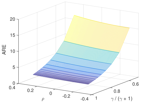
Figure 1: Plots of ARE as a function of $\gamma$ and $\rho$.

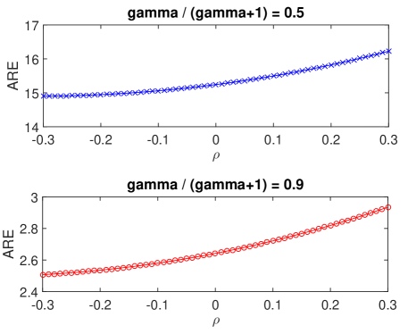
Figure 2: Plots of ARE as a function of $\rho$ for $\gamma=1$ and $\gamma=9$.

Fig. 1 plots the ARE at the pure-strategy NE as both the parameters $\rho$ and $\gamma$ are varied. There are two observations that we point out. First, it confirms that, for fixed $\gamma$, the ARE rises with increasing $\rho$ as predicted by Theorem 2. This can be seen more easily in Fig. 2, which displays the ARE as a function of $\rho$ for two different values of $\gamma$ ($\gamma=1$ and 9). Second, it is clear from Fig. 1 that as $\gamma$ increases, hence $\gamma/(\gamma+1)$ climbs, the ARE decreases quickly for all values of $\rho$ we considered. This hints at high sensitivity of the equilibrium ARE with respect to the cost effectiveness of available security measures.

In addition to corroborating Theorem 2, Fig. 2 reveals two additional interesting observations. First, it illustrates that the influence of network mixing (equivalently, parameter $\rho$) on ARE is more pronounced when the security measures are more cost effective (i.e., $\gamma$ is larger); when $\gamma=1$ (resp. $\gamma=9$), the ARE rises from 14.9 to 16.23 (resp. from 2.508 to 2.935) as $\rho$ ascends from -0.3 to 0.3, which is roughly an 8.9 percent increase (resp. a 17 percent increase). Therefore, they indicate that, although the equilibrium AREs are smaller when the security measures are more cost effective, they also become more sensitive to the bias in REs caused by assortativity.

Second, the ARE is a convex function of $\rho$. This hints that the impact of degree correlations on ARE gets stronger as the dependence graph becomes more assortative. As a result, a drop in ARE a disassortative dependence graph enjoys may not be as large as an increase in ARE an assortative dependence graph suffers. This in turn suggests that social networks, which in general exhibit non-negligible positive degree correlations [28, 29], may experience significant deterioration in security relative to the findings obtained using neutral networks.

VIII-B Effects of ARE function $\Theta$

In our second study, we explore how the ARE function $\Theta$ in (4) affects equilibrium ARE. In particular, we are interested in how sensitive the ARE is to the assortativity of dependence graph as we vary the shape of the function $\Theta$.

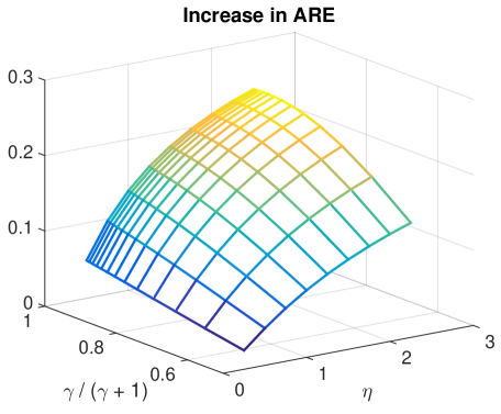
Figure 3: Plots of the increase in ARE as a function of $\gamma$ and $\eta$.

To this end, we adopt a family of functions of the form $\Theta(z)=K^{\prime}(\eta)z^{\eta}$ with $K^{\prime}(\eta),\eta>0$, where the parameter $\eta$ is used to change the shape of the function $\Theta$. In order to compare the ARE as we vary $\eta$, we adjust the value of parameter $K^{\prime}(\eta)$ as a function of $\eta$ so that the equilibrium ARE is identical under the neutral dependence graph (i.e., $\rho=0$) with $\gamma=5$ (equivalently, $\gamma/(\gamma+1)=0.8\bar{3}$) for all values of $\eta$ we consider.

Fig. 3 plots the increase in ARE as we vary $\rho$ from -0.3 to 0.3 for different values of $(\gamma,\eta)$. More precisely, each point in the figure represents the difference in ARE for $\rho=$ 0.3 and -0.3, divided by the value of ARE for $\rho=-0.3$.

It is clear from Fig. 3 that when $\gamma/(\gamma+1)$ is larger (indicating that the security measures are more cost effective), the ARE is more sensitive to assortativity because the relative increase in ARE is greater for all considered values of $\eta$. This confirms our finding in the previous subsection (illustrated by Fig. 2).

More importantly, Fig. 3 reveals that assortativity has greater impact on ARE when the ARE function $\Phi$ is more sensitive to the vulnerability of neighbors summarized by $\sum_{d\in{\mathcal{D}}}w_{d}({\bf s})\ p(a_{d})$. This observation is somewhat intuitive; as ARE becomes more sensitive to the vulnerability of agents, any changes in the security investments of agents will likely amplify the effects other parameters, including the assortativity of dependence graph.

IX Conclusion

We studied the effects of degree correlations on network security in IDS. Our findings reveal that the network security degrades when agents with larger degrees experience higher risks than those with smaller degrees. Moreover, somewhat unexpectedly, the cost effectiveness of available security measures determines how network mixing influences network security. Finally, our numerical studies suggest that as the infection probability or the vulnerability of neighboring agents becomes more sensitive to security investments, assortativity exerts greater impact on network security. Our analytical study carried out only a local analysis around neutral dependence graphs. We are currently working to generalize our results beyond the local neighborhood of neutral graphs.

References

- [1] R. Albert, H. Jeong and A.-L. Barabsi, “Error and attack tolerance of complex networks,” Nature, 406:378-382, Jul. 2000.
- [2] G. Bagler and S. Sinha, “Assortative mixing in protein contact networks and protein folding kinetics,” Bioinformatics, 23(14):1760-1767, 2007.
- [3] Y. Baryshnikov, “IT security investment and Gordon-Loev’s rule,” Proc. of the 11th Annual Workshop on the Economics of Information Security (WEIS), Berlin (Germany), Jun. 2012.
- [4] N. Beale, D.G. Rand, H. Battey, K. Croxson, R.M. May and M.A. Nowak, “Individual versus systemic risk and the regulator’s dilemma,” Proceedings of the National Academy of Sciences of the United States of America (PNAS), 108(31):12647-12652, Aug. 2011.
- [5] M. Bogu, R. Pastor-Satorras and A. Vespignani, “Absence of epidemic threshold in scale-free networks with degree correlations,” Phys. Rev. Lett., 90(2), 028701, Jan. 2003.
- [6] M. Bogu, R. Pastor-Satorras and A. Vespignani, “Epidemic spreading in complex networks with degree correlations,” Lecture Notes in Physics, 625:127-147, Sep. 2003.
- [7] J.C. Bolot and M. Lelarge, “A new perspective on Internet security using insurance,” Proc. of IEEE INFOCOM, Phoenix (AZ), Apr. 2008.
- [8] E. Bou-Harb, C. Fachkha, M. Pourzandi, M. Debbabi, and C. Assi, “Communication security for smart grid distribution networks,” IEEE Communications Magazine, 51(1):42-49, Jan. 2013.
- [9] F. Caccioli, T.A. Catanach, and J.D. Farmer, “Heterogeneity, correlations and financial contagion,” arXiv:1109.1213, Sep. 2011.
- [10] F. Caccioli, T.A. Catanach, and J.D. Farmer, “Stability analysis of financial contagion due to overlapping portfolios,” arXiv:1210.5987, Oct. 2012.
- [11] E. Coupechoux and M. Lelarge, “How clustering affects epidemics in random networks,”’ Advances in Applied Probability, 46(4):985-1008.
- [12] K.G. Gkonis and H.N. Psaraftis, “Container transportation as an interdependent security problem,” Journal of Transportation Security, 3(4):197-211, Dec. 2010.
- [13] G. Heal, H.C. Kunreuther and P.R. Orszag, “Interdependent security: Implications for homeland security policy and other areas,” Brookings Policy Brief Series, #108, Oct. 2002.
- [14] L. Jiang, V. Anantharam and J. Walrand, “How bad are selfish investments in network security?”, IEEE/ACM Trans. on Networking, 19(2):549-560, Apr. 2011.
- [15] S. Kakutani, “A generalization of Brouwer’s fixed point theorem,” Duke Mathematical Journal, 8(3):457-459, 1941.
- [16] M. Kearns and L.E. Ortiz, “Algorithms for interdependent security games,” Advances in Neural Information Processing Systems 16, 2003.
- [17] H. Kunreuther and G. Heal, “Interdependent Security,” The Journal of Risk and Uncertainty, 26(2/3):231-249, 2003.
- [18] H.C. Kunreuther and E.O. Michel-Kerjan, “Assessing, managing and benefiting from global interdependent risks: The case of terrorism and natural disasters,” Global Business and the Terrorist Threat, edited by H.W. Richardson, P. Gordon and J.E. Moore, Edward Elgar Publishing, 2009.
- [19] R.J. La, “Role of network topology in cybersecurity,” Proc. of IEEE Conference on Control and Decision (CDC), Los Angeles (CA), Dec. 2014.
- [20] R.J. La, “Interdependent security with strategic agents and global cascades,” IEEE/ACM Trans. on Networking (ToN), 24(3):1378-1391, Jun. 2016.
- [21] R.J. La, “Internalization of externalities in interdependent security: large network cases,” available at http://arxiv.org/abs/1703.01380.
- [22] R.J. La, “Influence of network mixing on interdependent security: local analysis,” Proc. of IEEE Globecom, Washington D.C., Dec. 2016.
- [23] A. Lakhina, J. Byers, M. Crovella and P. Xi, “Sampling biases in IP topology measurements,”’ Proc. of IEEE INFOCOM, San Francisco (CA), Apr. 2003.
- [24] A. Laszka, M. Felegyhazi and L. Buttyn, “A survey of interdependent information security games,” ACM Computing Surveys, 47(2):23:1-23:38, Jan. 2015.
- [25] M. Lelarge and J. Bolot, “A local mean field analysis of security investments in networks,” Proc. of the 3rd International Workshop on Economics of Networked Systems (NetEcon), pp. 25-30, Seattle (WA), Aug. 2008.
- [26] M. Lelarge and J. Bolot, “Economic incentives to increase security in the Internet: the case for insurance,” Proc. of IEEE INFOCOM, Rio de Janeiro (Brazil), Apr. 2009.
- [27] “Sampling from large graphs,” Proc. of ACM Knowledge Discovery and Data Mining (KDD), Philadelphia (PA), Aug. 2006.
- [28] M.E.J. Newman, “Assortative mixing in networks,” Phys. Rev. Lett., 89, 208701, Oct. 2002.
- [29] M.E.J. Newman, “Mixing patterns in networks,” Phys. Rev. E, 67, 026126, Feb. 2003.
- [30] R. Pastor-Satorras and A. Vespignani, “Epidemics and immunization in scale-free networks,” Handbook of Graphs and Networks: From the Genome to the Internet, Wiley, 2005.
- [31] M. Piraveenan, M. Prokopenko and A. Zomaya, “Assortative mixing in directed biological networks,” IEEE/ACM Trans. on Computational Biology and Bioinformatics, 9(1):66-78, Jan. 2012.
- [32] W. Rudin, The Principles of Mathematical Analysis, third ed., McGraw-Hill, 1976.
- [33] W.H. Sandholm Population Games and Evolutionary Dynamics, The MIT Press, 2010.
- [34] C.M. Schneider, M. Tamara, H. Shlomo and H.J. Herrmann, “Suppressing epidemics with a limited amount of immunization units,” Phys. Rev. E, 84, 061911, Dec. 2011.
- [35] M. Shaked and J.G. Shanthikumar, Stochastic Orders, Springer Series in Statistics, Springer, 2007.
- [36] C. Shapiro and H.R. Varian, Information Rules, Harvard Business School Press, 1999.
- [37] H.R. Varian, Microeconomic Analysis, 3rd edition, W.W. Norton & Company, 1992.
- [38] T.-F. Yen and M.K. Reiter, “Revisiting botnet models and their implications for takedown strategies,” Lecture Notes in Computer Science, 7215, pp. 249-268, 2012.
- [39] X. Zhao, L. Xue and A.B. Whinston, “Managing interdependent information security risks: cyberinsurance, managed security services, and risk pooling arrangements,” Proc. of International Conference on Information Systems (ICIS), Phoenix (AZ), 2009.
- [40] D. Zhou, H.E. Stanley, G. D’Agostino and A. Scala, “Assortativity decreases the robustness of interdependent networks,” Phys. Rev. E, 86, 066103, 2012.