Abstract

Spin-charge interconversion is currently the focus of intensive experimental and theoretical research both for its intrinsic interest and for its potential exploitation in the realization of new spintronic functionalities. Spin-orbit coupling is one of the key microscopic mechanisms to couple charge currents and spin polarizations. The Rashba spin-orbit coupling in a two-dimensional electron gas has been shown to give rise to the inverse spin galvanic effect, i.e. the generation of a non-equilibrium spin polarization by a charge current. Whereas the Rashba model may be applied to the interpretation of experimental results in many cases, in general in a given real physical system spin-orbit coupling also occurs due other mechanisms such as Dresselhaus bulk inversion asymmetry and scattering from impurities. In this work we consider the inverse spin galvanic effect in the presence of Rashba, Dresselhaus and impurity spin-orbit scattering. We find that the size and form of the inverse spin galvanic effect is greatly modified by the presence of the various sources of spin-orbit coupling. Indeed, spin-orbit coupling affects the spin relaxation time by adding the Elliott-Yafet mechanism to the Dyakonov-Perel and, furthermore, it changes the non-equilibrium value of the current-induced spin polarization by introducing a new spin generation torque. We use a diagrammatic Kubo formula approach to evaluate the spin polarization-charge current response function. We finally comment about the relevance of our results for the interpretation of experimental results.

x 10.3390/—— xx Received:Inverse spin galvanic effect in the presence of impurity spin-orbit scattering: a diagrammatic approach Amin Maleki and Roberto Raimondi^⋆Amin Maleki, and Roberto Raimondi Correspondence: email: roberto.raimondi@uniroma3.it; Tel. +39 06 5733 7032

1 Introduction

The spin galvanic effect and its inverse manifestation have been intensively investigated over the past decade both for their intrinsic fundamental interest Ganichev et al. (2016) and for their application potential in future generation electronic and spintronics technology Ando and Shiraishi (2017); Soumyanarayanan et al. (2016). The non-equilibrium generation of a spin polarization perpendicular to an externally applied electric field is referred to as the inverse spin galvanic effect (ISGE), whereas the spin galvanic effect (SGE) is its Onsager reciprocal, whereby a spin polarization injected through a nonmagnetic material creates a charge current in the direction perpendicular to the spin polarization. As an all-electrical method of generating and detecting spin polarization in nonmagnetic materials, both these effects may be used for applications such as spin-based field effect transistors Gardelis et al. (1999); Sarma et al. (2001); Sugahara and Tanaka (2005); Koo et al. (2009) and magnetic random access memory (MRAM) Miyazaki and Tezuka (1995); Yuasa Shinji et al. (2004).

The ISGE, also known as Edelstein effect or current-induced spin polarization, was originally proposed by Ivchenko and Pikus Ivchenko and Pikus (1978), and observed by Vorob’ev et al. in tellurium Vorob’ev et al. (1979). Later the ISGE was theoretically analyzed by Edelstein in a two-dimensional electron gas (2DEG) with Rashba spin-orbit coupling (SOC) Edelstein (1990) and also by Lyanda-Geller and AronovAronov and Lyanda-Geller (1989). Notice that the SGE in the spin-charge conversion is sometimes referred to as the inverse Rashba-Edelstein effect. The SGE has been observed experimentally in GaAs QWs by Ganichev et al. Ganichev S. D. et al. (2002), where the spin polarization was detected by measuring the current produced by circularly polarized light. In semiconducting structures the ISGE can be measured by optical methods such as Faraday rotation, linear-circular dichroism in transmission of terahertz radiation and time resolved Kerr rotation Ganichev et al. (2001, 2006); Yang et al. (2006); Ganichev et al. (2016). Very recently, a new way of converting spin to charge current has been experimentally developed by Rojas-Sánchez et al., where, by the spin-pumping technique, the non-equilibrium spin polarization injected from a ferromagnet into a silver (Ag)/Bismuth (Bi) interface yields an electrical current Sánchez et al. (2013). Successively, the SGE has also been observed in many interfaces with strong spin-orbit splitting, including metals with semiconductor giant SOC or insulator such as Fe/GaAs Chen et al. (2016), $Cu/Bi_{2}O_{3}$Karube et al. (2016).

Generally speaking, the SGE can be understood phenomenologically by symmetry arguments. Electrical currents and spin polarizations are polar and axial vectors, respectively. In centro-symmetric systems, polar and axial vectors transform differently and no SGE effect is expected. In restricted symmetry conditions, however, polar and axial vectors components may transform similarly. Consider, for instance, the case of electrons confined in the xy plane with the mirror reflection through the yz plane. Under such a symmetry operation, the electrical currents along the the x and y directions transform as $J_{x}\rightarrow-J_{x}$ and $J_{y}\rightarrow J_{y}$. The spin polarizations transform as the components of angular momentum, and we have $S^{y}\rightarrow-S^{y}$ and $S^{x}\rightarrow S^{x}$. Hence, one expects a coupling between $J_{x}$ and $S^{y}$ or between $J_{y}$ and $S^{x}$. Such a coupling is the SGE.

At microscopic level the strength of the coupling is due to the SOC. Usually the SOC is classified as extrinsic and intrinsic, depending on the origin of the electrical potential. The intrinsic SOC arises due to the crystalline potential of the host material or due the confinement potential associated with the device structure. On the other hand, the extrinsic SOC is due to the atomic potential of random impurities, which determine the transport properties of a given material. The majority of the studies on SGE/ISGE has focused on the Rashba SOC (RSOC) for electrons moving in the xy plane, which was originally introduced by Rashba Rashba (1960) to study the properties of the energy spectrum of non-centrosymmetric crystals of the CdS type and later successfully applied to the interpretation the two-fold spin splitting of electrons and holes in asymmetric semiconducting heterostructures Bychkov and Rashba (1984). RSOC is classified as due to structure inversion asymmetry (SIA), which is responsible for the confinement of electrons in the xy plane. In addition one may also consider the SOC arising from the bulk inversion asymmetry (BIA), usually referred to as Dresselhaus SOC (DSOC) Winkler (2003). Both RSOC and DSOC modify the energy spectrum by introducing a momentum-dependent spin splitting. This also can be understood quite generally on the basis of symmetry considerations. In a solid spin degneracy for a couple of states with opposite spin and with cristalline wave vector ${\bf k}$ is the result of both time reversal invariance and parity (space inversion invariance). By breaking the parity, as for instance, in a confined two-dimensional electron gas, the spin degeneracy is lifted and the Hamiltonian acquires an effective momentum-dependent magnetic field, which is the SOC. As a result electron states can be classified with their chirality in the sense that their spin state depends on their wave vector. In a such a situation, scalar disorder, although not directly acting on the spin state, influences the spin dynamics by affecting the wave vector of the electrons and holes. Spin relaxation arising in this context is usually referred to as the Dyakonov-Perel (DP) mechanism.

Extrinsic SOC originates from the potential which is responsible for the scattering from an impurity. In this case, before and after the scattering event, there is no direct connection between the wave vector and the spin of the electron. The scattering amplitude can be divided in spin-independent and spin-dependent contributions

$$S_{{\bf p},{\bf p}^{\prime}}=A+{\hat{\bf p}}\times{\hat{\bf p}^{\prime}}\cdot{\boldsymbol{\sigma}}B,$$ (1)

where $\hat{\bf p}$ and $\hat{\bf p}^{\prime}$ are the unit vector along the direction of the momentum before and after the scattering and ${\boldsymbol{\sigma}}$ is the vector of the Pauli matrices. As explained in Ref.Lifshits and Dyakonov (2009), different combinations of the amplitudes $A$ and $B$ correspond to specific physical processes. The $|A|^{2}+|B|^{2}$ describes the total scattering rate, whereas $|B|^{2}$ is associated to the Elliott-Yafet (EY) spin relaxation rate. Interference terms between the two amplitudes yield coupling among the currents. More in detail, the combination $AB^{*}+A^{*}B$ describes the skew scattering, which is responsible for the coupling between the charge and spin currents, whereas $AB^{*}-AB^{*}$ gives rise to the swapping of spin currents.

As noted in Ref.Ganichev et al. (2016), when both intrinsic and extrinsic SOC is present, the non-equilibrium spin polarization of the ISGE depends on the ratio of the DP and EY spin relaxation rates. This was analyzed in Ref.Raimondi et al. (2012) by means of the Keldysh non-equilibrium Green function within a SU(2) gauge theory-description of the SOC. Successively, a parallel analysis by standard Feynman diagrams for the Kubo formula was carried out in Ref.Maleki et al. (2016). These theoretical studies indeed confirmed that the ratio of DP to EY spin relaxation is able to tune the value of the ISGE. Such tuning is also affected by the value of the spin Hall angle due to the fact that spin polarization and spin current are coupled in the presence of intrinsic RSOC.

Recently, it has been shown theoretically Gorini et al. (2017) that the interplay of intrinsic and extrinsic SOC gives rise to an additional spin torque in the Bloch equations for the spin dynamics and affects the value of the ISGE. This additional spin torque, which is proportional to both the EY spin relaxation rate and to the coupling constant of RSOC, in Ref.Gorini et al. (2017) has been derived in the context of the SU(2) gauge theory formulation mentioned above. Although the SU(2) gauge theory is a very powerful approach, in order to emphasize the physical origin of this new torque it is very useful to show also how the same result can be obtained independently by using the diagrammatic approach of the Kubo linear response theory. This is the aim of the present paper.

In this paper we obtain an analytical formula of the ISGE in the presence of the Rashba, Dresselhaus and impurity SOC. In a 2DEG we will show that the intrinsic and extrinsic SOC act in parallel as far as relaxation to the equilibrium state is concerned.

The model Hamiltonian for a 2DEG in the presence of SOC reads

$$H=\frac{p^{2}}{2m}+\alpha(p_{y}\sigma_{x}-p_{x}\sigma_{y})+\beta(p_{x}\sigma_{x}-p_{y}\sigma_{y})+V({\bf r})-\frac{\lambda_{0}^{2}}{4}\nabla V({\bf r})\times{\bf p}\cdot\mbox{\boldmath$\sigma$},$$ (2)

where ${\bf p}=(p_{x},p_{y})$ is the vector of the components of the momentum operator, $\mbox{\boldmath$\sigma$}=(\sigma_{x},\sigma_{y},\sigma_{z})$ and ${\bf r}$ are the Pauli matrices and the coordinate operators. $m$ is the effective mass, $\alpha$ and $\beta$ are the Rashba and Dresselhaus SOC constants. $V({\bf r})$ represents a short-range impurity potential and finally $\lambda_{0}$ is the effective Compton wave length describing the strength of the extrinsic SOC. We assume the standard model of white-noise disorder potential with $\langle V({\bf r})\rangle=0$ and Gaussian distribution given by $\langle V({\bf r})V({\bf r}^{\prime})\rangle=n_{i}v_{0}^{2}\delta({\bf r}-{\bf r}^{\prime})=(\hbar/(2\pi N_{0}\tau_{0}))\delta({\bf r}-{\bf r}^{\prime})$. $N_{0}=m/2\hbar^{2}\pi$, $n_{i}$ and $v_{0}$ are the single-particle density of states per spin in the absence of SOC, the impurity concentration and the scattering amplitude, respectively. $\tau_{0}$ is the elastic scattering time at the level of the Fermi Golden Rule. From now on we work with units such that $\hbar=1$.

The layout of the paper is as follows. In the next Section we formulate the ISGE (the SGE can be obtained similarly by using the Onsager relations) in terms of the Kubo linear response theory. In Section 3 we derive an expression for the ISGE in the presence of the RSOC and extrinsic SOC. This case with no DSOC, whereas it is important by itself, allows to understand the origin of the additional spin torque in a situation which technically simpler to treat with respect to the general case when both RSOC and DSOC are different from zero. In Section 4, we expand our result to the specific case when the both RSOC and DSOC, as well as SOC from impurities, are present. We show how our result can be seen as the stationary solution of the Bloch equations for the spin dynamics. We comment briefly on the relevance of our result for the interpretation of the experiments. Finally, we state our conclusions in Section 5.

2 Linear response theory

In this Section we use the standard Kubo formula of linear response theory to derive the ISGE in the presence of extrinsic and intrinsic SOC. The in-plane spin polarization to linear order in the electric fields is given by

$$S^{i}=\sigma^{ij}_{EC}E_{j},\ i,j=x,y,$$ (3)

where $E_{i}$ is the external electric fields with frequency $\omega$ and $\sigma^{ij}_{EC}$ is the frequency-dependent "Edelstein conductivity"Edelstein (1990) given by the Kubo formula Shen et al. (2014)

$$\sigma^{ij}_{EC}(\omega)=\frac{(-e)}{2\pi}\sum\limits_{{\bf p}}{\rm Tr}[G^{A}(\epsilon+\omega)\Upsilon_{i}(\epsilon,\omega))G^{R}(\epsilon)J_{j}],$$ (4)

where the trace symbol includes the summation over spin indices. We keep the frequency dependence of $\sigma^{ij}_{EC}(\omega)$ in order to obtain the Bloch equations for the spin dynamics. In Eq.(4), $\Upsilon_{i}(\epsilon,\omega)$ is the renormalized spin vertex relative to a polarization along the $i$ axis, required by the standard series of ladder diagrams of the impurity technique Schwab and Raimondi (2002); Raimondi and Schwab (2005). $J_{j}$ are the bare number current vertices. In the plane-wave basis their matrix element from state ${\bf p}^{\prime}$ to state ${\bf p}$ read

$$J_{x} = \delta_{{\bf p},{\bf p}^{\prime}}\left(\frac{p_{x}}{m}-\alpha\sigma_{y}+\beta\sigma_{x}\right)+\delta j_{x,{\bf p}{\bf p}^{\prime}},$$ (5)

$$J_{y} = \delta_{{\bf p},{\bf p}^{\prime}}\left(\frac{p_{y}}{m}+\alpha\sigma_{x}-\beta\sigma_{y}\right)+\delta j_{y,{\bf p}{\bf p}^{\prime}}.$$ (6)

The latter term $\delta J_{j,{\bf p}{\bf p}^{\prime}}$ in Eqs.(5-6), which depends explicitly on disorder, is of order $\lambda_{0}^{2}$ and originates from the last term in the Hamiltonian of Eq.(2). Such a term gives rise to the side-jump contribution to the spin Hall effect Engel et al. (2005); Tse and Das Sarma (2006) due to the extrinsic SOC. The side-jump and skew-scattering contributions to the spin Hall effect in the presence of RSOC have been considered in Ref.Raimondi and Schwab (2009, 2010); Raimondi et al. (2012). A similar analysis of the side-jump and skew-scattering contributions to the ISGE has been carried out within the SU(2) gauge theory formualtion in Ref.Raimondi et al. (2012) and, more recently, in Ref.Maleki et al. (2016) by standard Kubo formula diagrammatic methods. For this reason we will not repeat such an analysis here, where instead we concentrate on the contributions generated by the first term on the right hand side of Eq.(5-6).

Within the self-consistent Born approximation, the last two terms of the Hamiltonian (2) yield an effective the self-energy when averaging over disorder. The self-energy is diagonal in momentum space and has two contributions due to the spin independent and spin dependent scattering Edelstein (1990); Shen et al. (2014)

$$\Sigma^{R}_{tot}({\bf p}) \equiv \Sigma^{R}_{0}({\bf p})+\Sigma^{R}_{EY}({\bf p})$$ (7)

$$= n_{i}v_{0}^{2}\sum_{{\bf p}^{\prime}}G^{R}_{{\bf p}^{\prime}}+n_{i}v_{0}^{2}\frac{\lambda_{0}^{4}}{16}\sum_{{\bf p}^{\prime}}\sigma_{z}G_{{\bf p}^{\prime}}^{R}\sigma_{z}({\bf p}\times{\bf p}^{\prime})^{2}_{z}.$$

Whereas the imaginary part of the first term gives rise to the standard elastic scattering time

$${\it Im}\Sigma^{R}_{0}({\bf p})=-i2\pi N_{0}n_{i}v_{0}^{2}=-\frac{i}{2\tau_{0}},$$ (8)

The second one is responsible for the EY spin relaxation. From the point of view of the scattering matrix introduced in the previous Section (cf. Eq.(1)), the two self-energies contributions correspond to the Born approximation for the $|A|^{2}$ and $|B|^{2}$, respectively. Given the self-energy (7), the retarded Green function is also diagonal in momentum space and can be expanded in the Pauli matrix basis in the form

$$G_{{\bf p}}^{R}=G^{R}_{0}\sigma_{0}+G^{R}_{x}\sigma_{x}+G^{R}_{y}\sigma_{y},$$ (9)

where

$$G^{R}_{0} = \frac{G^{R}_{+}+G^{R}_{-}}{2}$$

$$G^{R}_{x} = (\alpha\hat{p}_{y}+\beta\hat{p}_{x})\frac{G^{R}_{+}-G^{R}_{-}}{2\gamma}$$

$$G^{R}_{y} = -(\alpha\hat{p}_{x}+\beta\hat{p}_{y})\frac{G^{R}_{+}-G^{R}_{-}}{2\gamma}.$$ (10)

In the above $G^{R}_{\pm}(\epsilon)=(\epsilon-\frac{p^{2}}{2m}\mp\gamma p+\frac{i}{2\tau_{\pm}})^{-1}$ is the Green function corresponding to the two branches in which the energy spectrum splits due to the SOC. The factor $\gamma^{2}=\alpha^{2}+\beta^{2}+2\alpha\beta\sin(2\phi)$ with $\hat{p}_{x}=\cos(\phi)$ and $\hat{p}_{y}=\sin(\phi)$ describes the dependence in momentum space of the SOC, when both RSOC and DSOC are present. Notice that inversion in the two-dimensional momentum space ($(p_{x},p_{y})\rightarrow(-p_{x},-p_{y})$) leaves the factor $\gamma$ invariant, since it corresponds to $\phi\rightarrow\phi+\pi$. As a consequence, $G_{x,y}\rightarrow-G_{x,y}$, whereas $G_{0}$ is invariant. This observation will turn out to be useful later when evaluating the renormalization of the spin vertices. The advanced Green function is easily obtained via the relation $G^{A}_{\pm}=(G^{R}_{\pm})^{*}$. In the expression for $G^{R}_{\pm}$, $\frac{1}{2\tau_{\pm}}$ is a band-dependent time relaxation and plays an important role in our analysis. In order to obtain this term we note that, after momentum integration over ${\bf p}^{\prime}$ in Eq.(7), the imaginary part of the retarded self-energy reads

$$\Sigma^{R}_{\pm}=-{\rm i}\frac{1}{2\tau_{0}}-{\rm i}\left(\frac{\lambda_{0}^{2}}{4}\right)^{2}\frac{1}{4\tau_{0}}p_{F}^{2}p^{2}_{\pm}\equiv-\frac{{\rm i}}{2\tau_{\pm}}$$ (11)

Above, we indicate with $p_{F}$ the Fermi momentum without RSOC and DSOC and with $p_{\pm}$ the $\gamma$-dependent momenta of the two spin-orbit split Fermi surfaces. To lowest order in the spin-orbit splitting we have

$$p_{\pm}=p_{F}(1\mp\frac{\gamma}{v_{F}}),$$ (12)

where $v_{F}=p_{F}/m$. The momentum factors originate from the square of the vector product in the second term of Eq.(7). The factor $p_{F}^{2}$ is due to the inner ${\bf p}^{\prime}$ momentum, which upon integration is eventually fixed at the Fermi surface in the absence of RSOC and DSOC. More precisely, when evaluating the momentum integral, one ends up by summing the contributions of the two spin-orbit split bands in such a way that the $\alpha$- and $\beta$-dependent shift of the two Fermi surfaces cancels in the sum. However, the outer ${\bf p}$ momentum remains unfixed. Its value will be fixed by the poles of the Green function in a successive integration over the momentum. Then, the $\gamma$-dependent relaxation times of the two Fermi surfaces read

$$\frac{1}{\tau_{\pm}}=\frac{1}{\tau}(1\mp\frac{\tau}{\tau_{EY}}\frac{\gamma}{v_{F}}),$$ (13)

where

$$\frac{1}{\tau}=\frac{1}{\tau_{0}}+\frac{1}{2\tau_{EY}},$$ (14)

with the standard expression for the EY spin relaxation rates

$$\frac{1}{\tau_{EY}}=\frac{1}{\tau_{0}}\left(\frac{\lambda_{0}p_{F}}{2}\right)^{4}.$$ (15)

In order to evaluate Eq.(4), we need the renormalized spin vertex $\Upsilon_{i}$ which has an expansion in Pauli matrices $\Upsilon_{i}=\sum_{\rho=0,1,2,3}\Upsilon_{i}^{\rho}\sigma_{\rho}$, with the bare spin vertices $\Upsilon^{(0)}_{i}=\sigma_{i}$. We have dropped the explicit dependence $\Upsilon_{i}(\epsilon,\omega)$ for simplicity’s sake. For vanishing RSOC or DSOC, symmetry tells that the renormalized spin vertices share the same matrix structure of the bare ones $\Upsilon_{i}\sim\sigma_{i}$. However, when both RSOC and DSOC are present, symmetry arguments again indicate that $\Upsilon_{x}$ and $\Upsilon_{y}$ are not simply proportional to $\sigma_{x}$ and $\sigma_{y}$, but acquire both $\sigma_{x}$ and $\sigma_{y}$ components. By following the standard procedure Shen et al. (2014), after projecting over the Pauli matrix components, the vertex equation reads

$$\Upsilon_{i}^{\rho}=\delta_{\rho i}+\frac{1}{2}\sum_{\mu\upsilon\lambda}I_{\mu\upsilon}{\rm Tr}[\sigma_{\rho}\sigma_{\mu}\sigma_{\lambda}\sigma_{\upsilon}]\Upsilon_{i}^{\lambda}+\frac{1}{2}\sum_{\mu\upsilon\lambda}J_{\mu\upsilon}{\rm Tr}[\sigma_{\rho}\sigma_{z}\sigma_{\mu}\sigma_{\lambda}\sigma_{\upsilon}\sigma_{z}]\Upsilon_{i}^{\lambda},$$ (16)

where

$$I_{\mu\upsilon}=\frac{1}{2\pi N_{0}\tau_{0}}\sum_{{\bf p}^{\prime}}G^{A}_{\mu}(\epsilon+\omega)G^{R}_{\upsilon}(\epsilon),\ J_{\mu\upsilon}=\frac{\tau_{0}}{2\tau_{EY}}I_{\mu\upsilon}.$$ (17)

Once the spin vertices are known, the "Edelstein conductivities" from Eq.(4) can be put in the form

$$\sigma^{ij}_{EC}=\Upsilon_{i}^{\rho}\Pi_{\rho j}$$ (18)

with the bare "Edelstein conductivities" given by

$$\Pi_{\rho j}=\frac{(-e)}{2\pi}\sum_{{\bf p}}{\rm Tr}[G^{A}(\epsilon+\omega)\frac{\sigma_{\rho}}{2}G^{R}(\epsilon)J_{j}].$$ (19)

The bare "Edelstein conductivities" are those one would obtain by neglecting the vertex corrections due to the ladder diagrams. It is useful to point that one could have adopted the alternative route to renormalize the number current vertices and use the bare spin vertices. Indeed, this was the route followed originally by Edelstein Edelstein (1990). Since, the renormalized number current vertices, in the DC zero-frequency limit, vanish Raimondi and Schwab (2005), the evaluation of the Edelstein conductivity reduces to a bubble with bare spin vertices and the current vertices in absence of RSOC and DSOC.

3 Inverse spin-galvanic effect in the Rashba model

To keep the discussion as simple as possible, in this Section we confine first to the case when only RSOC is present. We will derive the spin polarization, $S^{y}$, when an external electric field is applied along the $x$ direction. Then in the next Section we will evaluate the Bloch equation in the more general case when both RSOC and DSOC are present. In the case $\beta=0$, the renormalized spin vertex $\Upsilon^{y}$ is simply proportional to $\sigma_{y}$, which means $\Upsilon^{y}=\Upsilon^{y}_{y}\sigma^{y}$. Upon the integration over momentum in Eq.(16), only $I_{00}$ is non-zero and other eight possibilities of $(\mu,\nu)$ in $I_{\mu,\nu}$ are zero. The cases $(0,x/y)$, $(x/y,0)$, $(x,y)$ and $(y,x)$ vanish because of angle integration, whereas the two other cases $(x,x)$ and $(y,y)$ cancel each other after taking the trace in Eq.(16).

As a result we finally obtain (in the diffusive approximation $\omega\tau\ll 1$)

$$\Upsilon_{y}=\Upsilon_{y}^{y}\sigma^{y}=\frac{1}{1-I_{00}+J_{00}}\sigma^{y}=\frac{1-4i\omega\tau}{\frac{\tau}{\tau_{s}}-i\omega\tau}\sigma^{y}$$ (20)

where the integral $I_{00}$ has been evaluated in the appendix A

$$I_{00}=\left(\frac{1-3i\omega\tau-\frac{\tau}{\tau_{\alpha}}}{1-4i\omega\tau}\right)\left(\frac{\tau}{\tau_{0}}\right)$$ (21)

with the total spin relaxation rate being $\frac{1}{\tau_{s}}=\frac{1}{\tau_{EY}}+\frac{1}{\tau_{\alpha}}$. Here $1/\tau_{\alpha}=(2m\alpha)^{2}D$ defines the DP spin relaxation rate due to the RSOC. Notice that, in the absence of SOC the vertex becomes singular by sending to zero the frequency, signaling the spin conservation in that limit. One sees that the EY and DP relaxation rates simply add up. This gives then $\sigma^{yx}=\Upsilon_{y}^{y}\Pi_{yx}$. Physically, in the zero-frequency limit, the factor $\Upsilon_{y}^{y}=\tau_{s}/\tau$ counts how many impurity scattering events are necessary to relax the spin. In the diffusive regime $\tau_{s}\gg\tau$, i.e. many impurity scattering events are necessary to erase the memory of the initial spin direction.

By neglecting the contribution from the extrinsic SOC in the expression (5) for the current vertex, the bare conductivity $\Pi_{yx}$ naturally separates in two terms $\Pi^{(A)}_{yx}$ and $\Pi^{(B)}_{yx}$ due to the components $p_{x}/m$ and $-\alpha\sigma^{y}$ of the number current vertex. The expression for $\Pi^{(A)}_{yx}$ reads

$$\Pi^{(A)}_{yx} = (-e)\frac{1}{2\pi}\sum_{\bf p}{\rm Tr}\left[G^{A}(\epsilon+\omega)\frac{\sigma^{y}}{2}G^{R}(\epsilon)\frac{p_{x}}{m}\right]$$ (22)

$$= \frac{e}{4\pi m}\sum_{\bf p}\frac{p}{2}\left[G^{A}_{+}(\epsilon+\omega)G^{R}_{+}(\epsilon)-G^{A}_{-}(\epsilon+\omega)G^{R}_{-}(\epsilon)\right]$$

$$= \frac{e}{4m}\left(\frac{p_{+}N_{+}}{-i\omega+\frac{1}{\tau_{+}}}-\frac{p_{-}N_{-}}{-i\omega+\frac{1}{\tau_{-}}}\right).$$

In the above $p_{\pm}$, $N_{\pm}$ and $\tau_{\pm}$ refer to the Fermi momentum, density of states and quasiparticle time in the $\pm$-band. To order $\alpha/v_{F}$, one has

$$p_{\pm}=p_{F}(1\mp\alpha/v_{F}),\ N_{\pm}=N_{0}(1\mp\alpha/v_{F}).$$ (23)

By including the contribution of the quasiparticle time in the $\pm$-band from Eq.(13), one gets

$$\Pi^{(A)}_{yx}=S_{0}\left(\frac{1-\frac{\tau}{2\tau_{EY}}-i\omega\tau}{1-2i\omega\tau}\right),$$ (24)

where $S_{0}=-eN_{0}\alpha\tau$. The evaluation of $\Pi^{(B)}_{yx}$ is more direct. It gives

$$\Pi^{(B)}_{yx} = \frac{e\alpha}{2\pi}\sum_{\bf p}{\rm Tr}\left[G^{A}(\epsilon+\omega)\frac{\sigma^{y}}{2}G^{R}(\epsilon)\sigma^{y}\right]$$ (25)

$$= \frac{e\alpha}{2\pi}\sum_{\bf p}\left(G^{A}_{0}(\epsilon+\omega)G^{R}_{0}(\epsilon)\right)$$

$$= -S_{0}\left(\frac{1-\frac{\tau}{\tau_{\alpha}}-3i\omega\tau}{1-4i\omega\tau}\right)$$

Combining both contributions with accuracy up to order $\omega\tau$ gives

$$\Pi_{yx}=\Pi^{(A)}_{yx}+\Pi^{(B)}_{yx}=S_{0}\left(\frac{\frac{\tau}{\tau_{\alpha}}-\frac{\tau}{2\tau_{EY}}}{1-6i\omega\tau}\right)$$ (26)

By combining the vertex correction Eq.(20) and the bare conductivity $\Pi_{yx}$ in Eq.(18), we get following contribution to the frequency-dependent spin polarization

$$(S^{y})^{(1)}=\frac{1}{(\frac{\tau}{\tau_{s}}-i\omega\tau)}\left(\frac{1-4i\omega\tau}{1-6i\omega\tau}\right)S_{\alpha}^{x}\left(\frac{\tau}{\tau_{\alpha}}-\frac{\tau}{2\tau_{EY}}\right).$$ (27)

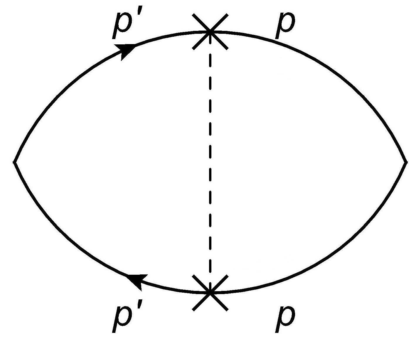
Figure 1: The diagram needed to evaluate the extra vertex correction to the ISGE due to extrinsic SOC. The left and right vertices denote the spin vertex $S^{y}$ and the component $(p_{x}/m)$ of the number current vertex $J_{x}$, whereas, the crosses on the top and bottom Green functions line stand for $-i(\lambda_{0}^{2}/4){\bf p}^{\prime}\times{\bf p}$ and $-i(\lambda_{0}^{2}/4){\bf p}\times{\bf p}^{\prime}$, respectively.

with $S_{\alpha}^{x}=-eN_{0}\alpha\tau E_{x}$. This is not the full story yet as we are to explain. What we have learned up to now is that the momentum dependence of the EY self-energy on the two spin-split Fermi surfaces yields an extra term to the Edelstein polarization. Such a momentum dependence can also modify the vertex corrections (the integrals $J_{\mu\upsilon}$ in Eq.(17)), which lead to the renormalized spin vertex. To appreciate this aspect we notice that in evaluating such integrals in the absence of the RSOC, the moduli of ${\bf p}$ and ${\bf p^{\prime}}$ are taken at the unsplit Fermi surface. We emphasize that, instead, taking into account the momentum dependence on the Rashba-split Fermi surfaces one gets an extra contribution. Consider the diagram of Fig. 1. After integration over ${\bf p}^{\prime}$, the left side part of the diagram gives

$$-\frac{(\lambda_{0}^{2}/4)^{2}p_{F}^{2}p^{2}}{2\tau_{0}}\tau=-\frac{\tau}{2\tau_{EY}}\frac{p^{2}}{p_{F}^{2}}.$$

If we set $p=p_{F}$, we would recover the standard diagrammatic calculation in the absence of intrinsic RSOC. By combining the above left side with the rest of the diagram, one gets an additional contribution to the bare conductivity

$$(\delta\Pi) = -\frac{\tau}{2\tau_{EY}}\left(-\frac{e}{2\pi}\sum_{\bf p}\frac{p^{2}}{p_{F}^{2}}{\rm Tr}\left[G^{A}(\epsilon+\omega)\frac{\sigma^{y}}{2}G^{R}(\epsilon)\frac{p_{x}}{m}\right]\right)$$ (28)

$$= \frac{-\tau}{2\tau_{EY}}(\frac{e}{4mp_{F}^{2}})\left(\frac{p^{3}_{+}N_{+}}{-i\omega+\frac{1}{\tau_{+}}}-\frac{p^{3}_{-}N_{-}}{-i\omega+\frac{1}{\tau_{-}}}\right).$$

To this expression we must subtract the one obtained by replacing $p=p_{F}$, which is already accounted for in the ladder summation. Hence the extra vertex part ($\delta\Pi$) modifies the spin polarization to give the second contribution

$$(S^{y})^{(2)}=\frac{1}{\left({\frac{\tau}{\tau_{s}}-i\omega\tau}\right)}\left(\frac{1-4i\omega\tau}{1-6i\omega\tau}\right)S_{\alpha}^{x}\left(-\frac{\tau}{2\tau_{EY}}\right).$$ (29)

Hence, by summing the above result to Eq.(27), the total spin polarization reads

$$S^{y}=\frac{1}{\left(\frac{1}{\tau_{s}}-i\omega\right)}\left(1+\frac{2i\omega\tau}{1-6i\omega\tau}\right)S_{\alpha}^{x}\left(\frac{1}{\tau_{\alpha}}-\frac{1}{\tau_{EY}}\right)\approx\frac{1}{\left(\frac{1}{\tau_{s}}-i\omega\right)}S_{\alpha}^{x}\left(\frac{1}{\tau_{\alpha}}-\frac{1}{\tau_{EY}}\right).$$ (30)

In the diffusive regime, terms in $\omega\tau$ in the second round brackets on the right hand side of Eq.(30) which are responsible for higher-order frequency dependence, can be neglected. In the zero-frequency limit, the Eq.(30) has two main contributions described by the two terms in the last round brackets. The first term is responsible for the Edelstein result Edelstein (1990) due to the intrinsic SOC, whereas the second one, which arises to order $\lambda_{0}^{4}$, is an additional contribution to the spin polarization due to the extrinsic SOC. In the Rashba model without extrinsic SOC, only the first term is present and, indeed, Eq.(30) reduces to it when $\lambda_{0}=\omega=0$. After Fourier transforming, the above equation can be written in the form of the Bloch equation

$$\partial_{t}S^{y}=-\left(\frac{1}{\tau_{\alpha}}+\frac{1}{\tau_{EY}}\right)S^{y}+\left(\frac{1}{\tau_{\alpha}}-\frac{1}{\tau_{EY}}\right)S^{x}_{\alpha}.$$ (31)

The terms on the right hand side describe the various torques controlling the spin dynamics. The first term, which includes DP and EY contributions, is the spin relaxation torques, wheres the second term represent the spin generation torques. The above result coincides with that obtained in Ref.Gorini et al. (2017) by the SU(2) gauge theory formulation. We have then succeeded in showing by diagrammatic methods the origin of the EY-induced spin torque discussed by Ref.Gorini et al. (2017). In the next Section we will generalize this result to the case when both RSOC and DSOC are present.

4 Inverse spin-galvanic effect in the Rashba-Dresslhaus model

As we have seen in the previous Section, the size and form of the ISGE is greatly modified by the presence of the EY spin relaxation due to the extrinsic SOC. To analyze this fact more generally we focus here on the model with RSOC and DSOC as well as SOC from impurities. In order to evaluate Eq.(4) for the Edelstein conductivity, we need the renormalized spin vertex $\Upsilon_{i}$. For vanishing RSOC or DSOC, the renormalized spin vertices share the same matrix structure of the bare ones $\Upsilon_{i}\sim\sigma_{i}$. However, when both RSOC and DSOC are explicitly taken into account, $\Upsilon_{x}$ and $\Upsilon_{y}$ are not only simply proportional to $\sigma_{x}$ and $\sigma_{y}$, but also acquire components on both $\sigma_{x}$ and $\sigma_{y}$. By following the procedure shown in Eq.(16) and upon integration over momentum, the vertex equation for $\Upsilon_{y}$ reduces to

$$\begin{pmatrix}1-I_{00}+J_{00}&-2(I_{yx}-J_{yx})\\ -2(I_{xy}-J_{xy})&1-I_{00}+J_{00}\end{pmatrix}\begin{pmatrix}\Upsilon^{y}_{y}\\ \Upsilon^{x}_{y}\end{pmatrix}=\begin{pmatrix}1\\ 0\end{pmatrix}$$ (32)

while that for$\Upsilon_{x}$ is

$$\begin{pmatrix}1-I_{00}+J_{00}&-2(I_{xy}-J_{xy})\\ -2(I_{yx}-J_{yx})&1-I_{00}+J_{00}\end{pmatrix}\begin{pmatrix}\Upsilon^{y}_{x}\\ \Upsilon^{x}_{x}\end{pmatrix}=\begin{pmatrix}0\\ 1\end{pmatrix},$$ (33)

where

$$1-I_{00}+J_{00} \simeq \left(\frac{-i\omega+\langle\frac{1}{\tau_{\gamma}}\rangle+\frac{1}{\tau_{EY}}}{1-4i\omega\tau}\right)\tau$$ (34)

$$-2(I_{xy}-J_{xy}) \simeq \left(\frac{1-i\omega\tau}{1-4i\omega\tau}\right)\left(1-\frac{\tau}{\tau_{EY}}\right)\frac{2\tau}{\tau_{\alpha\beta}},$$

where $\langle\dots\rangle$ indicated the average over the momentum directions. The technical points of the calculation in Eq.(34) are given in appendix A at the end of the paper. In the diffusive regime, $\frac{1}{\tau_{\gamma}}=(2m\gamma)^{2}D$ and $\frac{1}{\tau_{\alpha\beta}}=(2m)^{2}\alpha\beta D$ are the Dyakonov-Perel (DP) relaxation rates due to the total intrinsic spin-orbit strength and the interplay of RSOC/DSOC, respectively. For vanishing DSOC, the Eq.(34) reduce to the same expression in Eq.(20) as expected in the Rashba model. However, with both RSOC and DSOC, spin relaxation is anisotropic and one needs to diagonalize the matrix in the left hand side of Eqs.(32-33). Such a matrix then identifies the spin eigenmodes. Having in mind to derive the Bloch equations governing to spin dynamics, we rewrite Eq.(3) by using Eq.(18)

$$\begin{pmatrix}S^{x}\\ S^{y}\end{pmatrix}=\begin{pmatrix}\Upsilon^{x}_{x}&\Upsilon^{y}_{x}\\ \Upsilon^{x}_{y}&\Upsilon^{y}_{y}\end{pmatrix}\sum_{j}\begin{pmatrix}\Pi_{xj}\\ \Pi_{yj}\end{pmatrix}E_{j}$$ (35)

where, by virtue of Eqs.(32-33)

$$\begin{pmatrix}\Upsilon^{x}_{x}&\Upsilon^{x}_{y}\\ \Upsilon^{y}_{x}&\Upsilon^{y}_{y}\end{pmatrix}^{-1}=\frac{\tau}{1-4i\omega\tau}\begin{pmatrix}-i\omega+\langle\frac{1}{\tau_{\gamma}}\rangle+\frac{1}{\tau_{EY}}&\frac{2}{\tau_{\alpha\beta}}(1-i\omega\tau)\\ \frac{2}{\tau_{\alpha\beta}}(1-i\omega\tau)&-i\omega+\langle\frac{1}{\tau_{\gamma}}\rangle+\frac{1}{\tau_{EY}}\end{pmatrix}.$$ (36)

In the diffusive regime we can safely neglect the factor $\omega\tau$ with respect to unity in the denominator in front of the matrix and in the off diagonal elements of the matrix. The quantities $\Pi_{\rho j}$ appearing in the right hand side of Eq.(35) can be evaluated by standard techniques. However, some care is required when evaluating the momenta due to the extrinsic SOC at the spin-split Fermi surfaces, as we did in Eq.(28). The final result for the bare conductivities reads

$$\Pi_{xx} = \frac{-\tau S_{\beta}^{x}}{1-6i\omega\tau}\langle\frac{1}{\tau_{\gamma}}-\frac{1}{\tau_{EY}}-\frac{2}{\tau_{\gamma}}\frac{\alpha^{2}}{\gamma^{2}}\rangle,$$ (37)

$$\Pi_{xy} = \frac{-\tau S_{\alpha}^{y}}{1-6i\omega\tau}\langle\frac{1}{\tau_{\gamma}}-\frac{1}{\tau_{EY}}-\frac{2}{\tau_{\gamma}}\frac{\beta^{2}}{\gamma^{2}}\rangle,$$ (38)

$$\Pi_{yx} = \frac{\tau S_{\alpha}^{x}}{1-6i\omega\tau}\langle\frac{1}{\tau_{\gamma}}-\frac{1}{\tau_{EY}}-\frac{2}{\tau_{\gamma}}\frac{\beta^{2}}{\gamma^{2}}\rangle,$$ (39)

$$\Pi_{yy} = \frac{\tau S_{\beta}^{y}}{1-6i\omega\tau}\langle\frac{1}{\tau_{\gamma}}-\frac{1}{\tau_{EY}}-\frac{2}{\tau_{\gamma}}\frac{\alpha^{2}}{\gamma^{2}}\rangle,$$ (40)

with

$$S_{\beta}^{x} = -eN_{0}\tau\beta E_{x}$$ (41)

$$S_{\alpha}^{y} = -eN_{0}\tau\alpha E_{y}$$ (42)

$$S_{\alpha}^{x} = -eN_{0}\tau\alpha E_{x}$$ (43)

$$S_{\beta}^{y} = -eN_{0}\tau\beta E_{y}..$$ (44)

We take the angular average over the DP relaxation rates in Eqs.(36-40)

$$\int\limits_{0}^{2\pi}\frac{d\phi}{2\pi}\frac{1}{\tau_{\gamma}}=\frac{1}{\tau_{\alpha}}+\frac{1}{\tau_{\beta}}$$ (45)

$$(-2)(\alpha^{2}\ {\rm or}\ \beta^{2})\int\limits_{0}^{2\pi}\frac{d\phi}{2\pi}\frac{1}{\tau_{\gamma}}\frac{1}{\gamma^{2}}=\frac{-2}{\tau_{\alpha}}\ {\rm or}\ \frac{-2}{\tau_{\beta}}.$$ (46)

where $\frac{1}{\tau_{\alpha}}=(2m\alpha)^{2}D$, $\frac{1}{\tau_{\beta}}=(2m\beta)^{2}D$ are the DP relaxation rates due to RSOC and DSOC in the diffusive approximation. By inserting the above expression into Eqs.(37-40) and vertex correction in Eq.(36) and using Eq.(35), we may write the expression of the ISGE components in a form reminiscent of the Bloch equations

$$\begin{pmatrix}-i\omega+\frac{1}{\tau_{\alpha}}+\frac{1}{\tau_{\beta}}+\frac{1}{\tau_{EY}}&\frac{2}{\tau_{\alpha\beta}}\\ \frac{2}{\tau_{\alpha\beta}}&-i\omega+\frac{1}{\tau_{\alpha}}+\frac{1}{\tau_{\beta}}+\frac{1}{\tau_{EY}}\end{pmatrix}\begin{pmatrix}S^{x}\\ S^{y}\end{pmatrix}=\begin{pmatrix}-S_{\alpha}^{y}(\frac{1}{\tau_{\alpha}}-\frac{1}{\tau_{\beta}}-\frac{1}{\tau_{EY}})-S_{\beta}^{x}(\frac{-1}{\tau_{\alpha}}+\frac{1}{\tau_{\beta}}-\frac{1}{\tau_{EY}})\\ S_{\alpha}^{x}(\frac{1}{\tau_{\alpha}}-\frac{1}{\tau_{\beta}}-\frac{1}{\tau_{EY}})+S_{\beta}^{y}(\frac{-1}{\tau_{\alpha}}+\frac{1}{\tau_{\beta}}-\frac{1}{\tau_{EY}})\end{pmatrix},$$ (47)

Indeed, by performing the anti-Fourier transform with respect to the frequency $\omega$, Eq.(47) can be written as

$$\partial_{t}{\bf S}=-(\hat{\Gamma}_{DP}+\hat{\Gamma}_{EY}){\bf S}+(\hat{\Gamma}_{DP}-\hat{\Gamma}_{EY})\frac{N_{0}}{2}{\bf B},$$ (48)

where ${\bf B}$ represents the internal SOC field induced by the electric current. The $\hat{\Gamma}_{DP}$ and $\hat{\Gamma}_{EY}$ are the DP and EY relaxation matrix

$${\bf B}=2e\tau\begin{pmatrix}\beta E_{x}+\alpha E_{y}\\ -(\alpha E_{x}+\beta E_{y})\end{pmatrix},\hat{\Gamma}_{DP}=\begin{pmatrix}\frac{1}{\tau_{\alpha}}+\frac{1}{\tau_{\beta}}&\frac{2}{\tau_{\alpha\beta}}\\ \frac{2}{\tau_{\alpha\beta}}&\frac{1}{\tau_{\alpha}}+\frac{1}{\tau_{\beta}}\end{pmatrix},\hat{\Gamma}_{EY}=\begin{pmatrix}\frac{1}{\tau_{EY}}&0\\ 0&\frac{1}{\tau_{EY}}\end{pmatrix}.$$ (49)

Eq.(48) is the main result of our paper. It shows that the intrinsic and extrinsic SOC act in parallel as far as relaxation to the equilibrium state is concerned, i.e. the DP and EY spin relaxation matrices add up. However, as far as the spin generation torques are concerned, DP and EY processes have opposite sign. This is in full agreement with the result of Ref.Gorini et al. (2017) once we take into account also the spin generation torque due to side-jump and skew-scattering processes discussed diagramatically in Ref.Maleki et al. (2016). This is simply obtained by multiplying the DP relaxation matrix $\hat{\Gamma}_{DP}$ in the second term in the right hand side of Eq.(48) by the factor $1+\theta^{sH}_{ext}/\theta^{sH}_{int}$, where $\theta^{sH}_{ext}$ and $\theta^{sH}_{int}$ are the spin Hall angles for extrinsic and intrinsic SOC.

To develop some quick intuition, one may notice that again for $\beta=\lambda_{0}=0$ and $E_{y}=\omega=0$, Eq.(47) reproduces the Edelstein result for the Rashba model Edelstein (1990). Furthermore, when also $\omega\neq 0$ it reproduces the frequency-dependent spin polarization for the Rashba model as shown in the previous Section. When $\lambda_{0}\neq 0$ and $\beta=0$, we see that the ISGE, due to the interplay of the extrinsic and intrinsic SOC, gets an additional spin torque, suggesting that the EY spin-relaxation is detrimental to the Edelstein effect. The diagrammatic analysis reported here provides the following interpretation. The EY spin relaxation depends on the Fermi momentum. When there are two Fermi surfaces with different Fermi momenta, the one with the smaller momentum undergoes less spin relaxation of the EY type than the one with larger momentum. On the other hand, the ISGE arises precisely because there is an unbalance among the two Fermi surfaces with respect to spin polarization. For a given momentum direction, the larger Fermi surface contributes more to the Edelstein polarization than the smaller Fermi surface. Hence, the combination of these two facts suggests a negative effect from the interplay of Edelstein effect and EY spin relaxation. By neglecting the EY relaxation, one sees that the DP terms can cancel each other if the RSOC and DSOC strengths are equal. This cancellation or anisotropy of the spin accumulation could be used to determine the absolute values of the RSOC and DSOC strengths under spatial combination of spin dependent relaxation.
Finally, we comment on the relevance of our theory with respect to existing experiments Ref.Norman et al. (2014). The latter show that the current-induced spin polarization does not align along the internal magnetic field ${\bf B}$ due to the SOC. According to our Eq.(48) this may occur due to the presence of the extrinsic SOC both in the spin relaxation torque and in the spin generation torque. Indeed when the extrinsic SOC is absent, the spin polarization must necessarily align along the ${\bf B}$ field. Hence, our theory could, in principle, provide a method to measure the relative strength of intrinsic and extrinsic SOC.

5 Conclusions

In this present work, we showed how the interplay of intrinsic and extrinsic spin-orbit coupling modifies the current-induced spin polarization in a 2DEG. This phenomenon, known as the inverse spin galvanic effect, is the consequence of the coupling between spin polarization and electric current, due to restricted symmetry conditions. We derived the frequency-dependent spin polarization response, which allowed us to obtain the Bloch equations governing the spin dynamics of carriers. We identified the various sources of spin relaxation. In fact, the precise relation between the non-equilibrium spin polarization and spin-orbit coupling depends on ratio of the DP and EY spin relaxation rates. More precisely, the spin-orbit coupling affects the spin relaxation time by adding the EY mechanism to the DP and, furthermore, it changes the non-equilibrium value of the current-induced spin polarization by introducing an additional spin torque. Our treatment, which is valid at the level of Born approximation and was obtained by diagrammatic technique agrees with the analysis of Ref.Gorini et al. (2017), derived via the quasiclassical Keldysh Green function technique. Finally, to make comparison between theory and experiments, we found that the spin polarization and internal magnetic field will not be aligned if the EY is strong enough.

one

Appendix A Integrals of products involving pairs of retarded and advanced Green functions

To perform the calculations of the renormalized spin vertex in Eq.(34) and also in all the analysis, we encounter the following kind of integrals, which are evaluated to first order in $\frac{\gamma}{v_{F}}$ and $\omega\tau$

$$\sum_{{\bf p}}p^{n}G^{R}_{\pm}(\epsilon+\omega)G^{A}_{\pm}(\epsilon) \approx 2\pi N_{\pm}p^{n}_{\pm}\frac{1}{-i\omega+\frac{1}{\tau_{\pm}}}$$ (50)

$$\sum_{{\bf p}}p^{n}G^{R}_{\pm}(\epsilon+\omega)G^{A}_{\mp}(\epsilon) \approx 2\pi N_{0}p^{n}_{\pm}\frac{1}{-i\omega\pm 2i\gamma p_{F}+\frac{1}{\tau}}$$ (51)

where $n=0,1$. We can then evaluate the $I_{00}$ integral as

$$I_{00} = \frac{1}{2\pi N_{0}\tau_{0}}\sum_{{\bf p}^{\prime}}G^{A}_{0}(\epsilon+\omega)G^{R}_{0}(\epsilon)$$ (52)

$$= \frac{1}{2\pi N_{0}\tau_{0}}\sum_{{\bf p}^{\prime}}\frac{1}{4}\left(G^{A}_{+}(\epsilon+\omega)G^{R}_{+}(\epsilon)+G^{A}_{+}(\epsilon+\omega)G^{R}_{-}(\epsilon)+G^{A}_{-}(\epsilon+\omega)G^{R}_{+}(\epsilon)+G^{A}_{-}(\epsilon+\omega)G^{R}_{-}(\epsilon)\right)$$

$$= \frac{1}{4N_{0}\tau_{0}}\langle\frac{N_{+}}{-i\omega+\frac{1}{\tau_{+}}}+\frac{N_{-}}{-i\omega+\frac{1}{\tau_{-}}}+\frac{N_{0}}{-i\omega+2ip_{F}\gamma+\frac{1}{\tau}}+\frac{N_{0}}{-i\omega-2ip_{F}\gamma+\frac{1}{\tau}}\rangle$$

$$\approx (\frac{\tau}{\tau_{0}})\left(\frac{1-3i\omega\tau-\langle\frac{\tau}{\tau_{\gamma}}\rangle}{1-4i\omega\tau}\right)$$

and the same calculations for $2I_{xy}=2I_{yx}$ yields

$$2I_{xy} = \frac{2}{2\pi N_{0}\tau_{0}}\sum_{{\bf p}^{\prime}}G^{A}_{x}(\epsilon+\omega)G^{R}_{y}(\epsilon)$$ (53)

$$= \frac{2}{2\pi N_{0}\tau_{0}}\left(\frac{-\alpha\beta}{4\gamma^{2}}\right)\sum_{{\bf p}^{\prime}}\left(G^{A}_{+}(\epsilon+\omega)G^{R}_{+}(\epsilon)-G^{A}_{+}(\epsilon+\omega)G^{R}_{-}(\epsilon)-G^{A}_{-}(\epsilon+\omega)G^{R}_{+}(\epsilon)+G^{A}_{-}(\epsilon+\omega)G^{R}_{-}(\epsilon)\right)$$

$$\approx (\frac{4\tau}{\tau_{0}})(\frac{2\tau}{\tau_{\gamma}})\left(\frac{-\alpha\beta}{4\gamma^{2}}\right)(\frac{1-i\omega\tau}{1-4i\omega\tau})$$

$$= \frac{2\tau}{\tau_{\alpha\beta}}(\frac{1-i\omega\tau}{1-4i\omega\tau}).$$