Block-Matching Convolutional Neural Network for Image Denoising

Abstract

There are two main streams in up-to-date image denoising algorithms: non-local self similarity (NSS) prior based methods and convolutional neural network (CNN) based methods. The NSS based methods are favorable on images with regular and repetitive patterns while the CNN based methods perform better on irregular structures. In this paper, we propose a block-matching convolutional neural network (BMCNN) method that combines NSS prior and CNN. Initially, similar local patches in the input image are integrated into a 3D block. In order to prevent the noise from messing up the block matching, we first apply an existing denoising algorithm on the noisy image. The denoised image is employed as a pilot signal for the block matching, and then denoising function for the block is learned by a CNN structure. Experimental results show that the proposed BMCNN algorithm achieves state-of-the-art performance. In detail, BMCNN can restore both repetitive and irregular structures.

I Introduction

With current image capturing technologies, noise is inevitable especially in low light conditions. Moreover, captured images can be affected by additional noises through the compression and transmission procedures. Since the noise degrades visual quality, compression performance, and also the performance of computer vision algorithms, the image denoising has been extensively studied over several decades [1, 2, 3, 4, 5, 6, 7, 8, 9, 10, 11, 12, 13].

In order to estimate a clean image from its noisy observation, a number of methods that take account of certain image priors have been developed. Among various image priors, the NSS is considered a remarkable one such that it is employed in most of current state-of-the-art methods. The NSS implies that some patterns occur repeatedly in an image and the image patches that have similar patterns can be located far from each other. The nonlocal means filter [1] is a seminal work that exploits this NSS prior. The employment of NSS prior has boosted the performance of image denoising significantly, and many up-to-date denoising algorithms [3, 14, 7, 15, 16] can be categorized as NSS based methods. Most NSS based methods consist of following steps. First, they find similar patches and integrate them into a 3D block. Then the block is denoised using some other priors such as low-band prior[3], sparsity prior[15, 16] and low-rank prior[7]. Since the patch similarity can be easily disrupted by noise, the NSS based methods are usually implemented as two-step or iterative procedures.

Although the NSS based methods show high denoising performance, they have some limitations. First, since the block denoising stage is designed considering a specific prior, it is difficult to satisfy mixed characteristics of an image. For example, some methods work very well with the regular structures (such as stripe pattern) whereas some do not. Furthermore, since the prior is based on human observation, it can hardly be optimal. The NSS based methods also contain some parameters that have to be tuned by a user, and it is difficult to find the optimal parameters for the overall tasks. Lastly, many NSS based methods such as LSSC[14], NCSR[5] and WNNM[7] involve complex optimization problems. These optimizations are very time-consuming, and also very difficult to be parallelized.

Some researchers, meanwhile, developed discriminative learning methods for image denoising, which learn the image prior models and corresponding denoising function. Schmidt et al.[17] proposed a cascade of shrinkage fields (CSF) that unifies the random field-based model and quadratic optimization. Chen et al. [18] proposed a trainable nonlinear reaction diffusion (TNRD) model which learns parameters for a diffusion model by the gradient descent procedure. Although these methods find optimal parameters in a data-driven manner, they are limited to the specific prior model. Recently, neural network based denoising algorithms [9, 2, 19] are attracting considerable attentions for their performance and fast processing by GPU. They trained networks which take noisy patches as input and estimate noise-free original patch. These networks consist of series of convolution operations and non-linear activations. Since the neural network denoising algorithms are also based on the data-driven framework, they can learn at least locally optimal filters for the local regions provided that sufficiently large number of training patches from abundant dataset are available. It is believed that the networks can also learn the priors which were neglected by human observers or difficult to be implemented. However, the patch-based denoising is basically a local processing and the existing neural network methods did not consider the NSS prior. Hence, they often show inferior performance than the NSS based methods especially in the case of regular and repetitive structures [20], which lowers the overall performance.

In this paper, a combined denoising framework named block-matching convolutional neural network (BMCNN) is presented. Fig. 1 illustrates the difference between the existing denoising algorithms and the proposed method. As shown in the figure, the proposed method finds similar patches and stack them as a 3D input like BM3D [3], which is illustreated in Fig. 1-(d). By using the set of similar patches as the input, the network is able to consider the NSS prior in addition to the local prior that the conventional neural networks could train. Compared to the conventional NSS based algorithms, the BMCNN is a data-driven framework and thus can find more accurate denoising function for the given input. Finally, it will be explained that some of the conventional methods can also be interpreted as a kind of BMCNN framework.

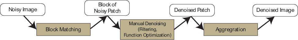
(a)

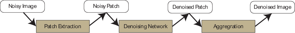
(b)

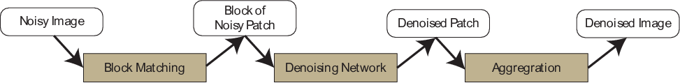
(c)

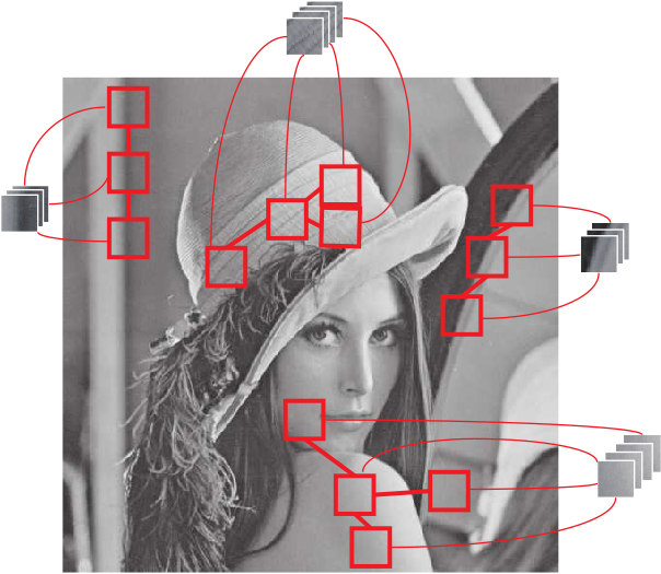
(d)

Figure 1: Flow chart of (a) conventional NSS based system, (b) NN based system and (c) the proposed BMCNN. (d) Illustration of block-matching step.

The rest of this paper is organized as follows. In Section II, researches that are related with the proposed framework are reviewed. There are two main topics: image denoising based on NSS, and image restoration based on neural network. Section III presents the proposed BMCNN network. In Section IV, experimental results and the comparison with the state-of-the-art methods are presented. This paper is concluded in Section V.

II Related works

II-A Image Denoising based on Nonlocal Self-similarity

Most state-of-the-art denoising methods [1, 3, 7, 21, 4] employ NSS prior of natural images. The nonlocal means filter (NLM)[1] was the first to employ this prior to estimate a clean pixel from the relations of similar non-neighboring blocks. Some other algorithms estimate the denoised patch rather than estimating each pixel separately. For instance, Dabov et al. [3] proposed the BM3D algorithm that exploits non-local similar patches for denoising a patch. The similar patches are found by block matching and they are stacked to be a 3D block, which is then denoised in the 3D transform domain. Dong et al. [4, 5] solved the denoising problem by using the sparsity prior of natural images. Since the matrix formed by similar patches is of low rank, finding the sparse representation of noisy group results in a denoised patch. Nejati et al. [15] proposed a low-rank regularized collaborative filtering. Gu et al. [7] also considered denoising as a kind of low-rank matrix approximation problem which is solved by weighted nuclear norm minimization (WNNM). In addition to the low-rank nature, they took advantage of the prior knowledge that large singular value of the low-rank approximation represents the major components of the image. Specifically, the WNNM algorithm adopted the term that prevents large singular values from shrinking in addition to the conventional nuclear norm minimization (NNM) [22]. Recently, Zha et al. [16] proposed to use group sparsity residual constraint. Their method estimates a group sparse code instead of denoising the group directly.

II-B Image restoration based on Neural Network

Since Lecun et al. [23] showed that their CNN performs very well in digit classification problem, various CNN structures and related algorithms have been developed for diverse computer vision problems ranging from low to high-level tasks. Among these, this section introduces some neural network algorithms for image enhancement problems. In the early stage of this work, some multilayer perceptrons (MLP) were adopted for image processing. Burger et al. [2] showed that a plain MLP can compete the state-of-the-art image denoising methods (BM3D) provided that huge training set, deep network and numerous neuron are available. Their method was tested on several type of noise: Gaussian noise, salt-and-pepper noise, compression artifact, etc. Schuler et al. [24] trained the same structure to remove the artifacts that occur from non-blind image deconvolution.

Meanwhile, many researchers have developed CNN based algorithms. Jain et al. [9] proposed a CNN for denoising, and discussed its relationship with the Markov random field (MRF) [25]. Dong et al. [26] proposed a SRCNN, which is a convolutional network for image super-resolution. Although their network was lightweight, it achieved superior performance to the conventional non-CNN approaches. They also showed that some conventional super-resolution methods such as sparse coding [27] can be considered a special case of deep neural network. Their work was continued to the compression artifact reduction[28]. Kim et al. [29, 30] proposed two algorithms for image super-resolution. In [30], they presented skip-connection from input to output layer. Since the input and output are highly correlated in super-resolution problem, the skip-connection was very effective. In [29], they introduced a network with repeated convolution layers. Their recursive structure enabled a very deep network without huge model and prevented exploding/vanishing gradients [31].

Recently, some techniques such as residual learning [32] and batch normalization [33] have made considerable contributions in developing CNN based image processing algorithms. The techniques contribute to stabilizing the convergence of the network and improving the performance. For some examples, Timofte et al. [34] adopted residual learning for image super-resolution, and Zhang et al. [19] proposed a deep CNN using both batch normalization and residual learning.

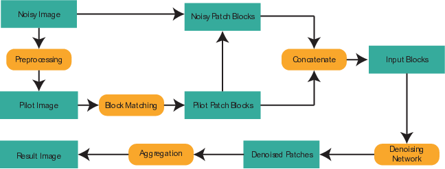
Figure 2: The flowchart of proposed BMCNN denoising algorithm.

III Block Matching Convolutional Neural Network

In this section, we present the BMCNN that esimtates the original image $X$ from its noisy observation $Y=X+V$, where we concentrate on additive white Gaussian noise (AWGN) that follows $V\sim N(0,\sigma^{2})$. The overview of our algorithm is illustrated in Fig. 2. First, we apply an existing denoising method to the noisy image. The denoised image is regraded as a pilot signal for block matching. That is, we find a group of similar patches from the input and pilot images, which is denoised by a CNN. Finally, the denoised patches are aggregated to form the output image.

III-A Patch Extraction and Block Matching

Many up-to-date denoising methods are the patch-based ones, which denoise the image patch by patch. In the patch-based methods, the overlapping patch ${\{y_{p}\}}$ of size $N_{patch}\times N_{patch}$ are extracted from $Y$, centered at the pixel position $p$. Then, each patch is denoised and merged together to form an output image. In general, this approach yields the best performance when all possible overlapping patches are processed, i.e., when the patches are extracted with the stride 1. However, this is obviously computationally demanding and thus many previous studies [3, 2, 7] suggested to use some larger stride that decreases computations while not much degrading the performance.

In the conventional NSS based algorithm [3], they first find similar patches to $y_{p}$ based on the dissimilarity measure defined as

$$d(y_{p},y_{q})=\lVert y_{p}-y_{q}\rVert^{2}.$$ (1)

Specifically, the $k$ patches nearest to $y_{p}$ including itself are selected and stacked, which forms a 3D block $\{Y_{p}\}$ of size $N_{patch}\times N_{patch}\times k$. Then the block is denoised in the 3D transform domain. However, it is also shown in [3] that the noise affects the block matching performance too much. Specifically, the distance with the noisy observation is a non-central chi-squared random variable with the mean

$$E(d(y_{p},y_{q}))=d(x_{p},x_{q})+2\sigma^{2}N_{patch}^{2}$$ (2)

and variance

$$V(d(y_{p},y_{q}))=8\sigma^{2}N_{patch}^{2}(\sigma^{2}+d(x_{p},x_{q})).$$ (3)

where $x_{p}$ and $x_{q}$ are clean image patches that corresnpond to $y_{p}$ and $y_{q}$ respectively. As shown, the variance grows with $O(\sigma^{4})$, and thus the block matching results are likely to depend more on the noise distribution as the $\sigma$ gets larger. This problem is somewhat alleviated by the two-step approach, i.e., they denoise the 3D block as stated above at the first step. Then, at the second step, the similar patches are again aggregated by using the denoised patch as a reference, and the denoised and original patches are stacked together to be denoised again.

In this respect, we also use a denoised patch to find its similar patches from the noisy and denoised image. Precisely, we adopt an existing denoising algorithm as a preprocessing step. The preprocessing step finds a denoised image $\hat{X}_{basic}$, which is named pilot image and used for our patch aggregation as follows:

• Block-matching is performed on $\hat{X}_{basic}$. Since the preprocessing attenuates the noise, the block-matching on the pilot image provides more accurate results.

• The group is formed by stacking both the similar patches in the pilot image and the corresponding noisy patches. Since some information can be lost by denoising, noisy input patch can help reconstructing the details of the image.

In this paper, we mainly use DnCNN [19] to find the pilot image because of its promising denoising performance and short run-time on GPU. We also use BM3D as a preprocessing step, which shows almost the same performance on the average. But the DnCNN and BM3D lead to somewhat different results for the individual image as will be explained in the experiment section.

III-B Network Structure

In CNN based methods, designing a network structure is an essential step that determines the performance. Simonyan et al. [35] pointed out that deep networks consisting of small convolutional filters with the size $3\times 3$ can achieve favorable performance in many computer vision tasks. Based on this principle, the DnCNN [19] employed only $3\times 3$ filters, and our network is also consisted of $3\times 3$ filters, with residual learning and batch normalization. The architecture of the network is illustrated in Fig. 3.

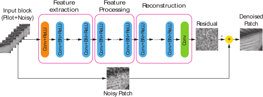
Figure 3: The architecture of the denoising network

(a)	(b)	(c)	(d)	(e)	(f)

Figure 4: Feature maps from the denoising network. (a) Patches in an input image (b) the output of the first conv layer (c) the output of the feature extraction stage (at the same time, the input to the feature processing stage) (d) the output of the feature processing stage (at the same time, the input to the reconstruction stage), (e) the input of the last layer, (f) the output residual patch.

In our algorithm, the depth is set to 17, and the network is composed of three types of layers. The first layer generates 64 low-level feature maps using 64 filters of size $3\times 3\times 2k$, for the $k$ patches from the input and another $k$ patches from the preprocessed image. Then, the feature maps are processed by a rectified linear unit (ReLU). The layers except for the first and the last layer (layer 2 $\sim$ 16) contain batch normalization between the convolution filters and ReLU operation. The batch normalization for feature maps is proven to offer some merits in many previous works [36, 33, 37], such as the alleviation of internal covariate shift. All the convolution operations for these layers use 64 filters of size $3\times 3\times 64$. The last layer consists of only a convolution layer. The layer uses a single $3\times 3\times 64$ filter to construct the output from the processed feature maps. In this paper, the network adopts the residual learning, i.e., $f(Y)=V$ [32] . Hence, the output of the last layer is the estimated noise component of the input and the denoised patch is obtained by subtracting the output from the input. These layers can also be categorized into three stages as follows.

III-B1 Feature Extraction

At the first stage (layer $1\sim 6$), the features of the patches are extracted. Figs. 4-(a)$\sim$(c) show the function of the stage. The first layer transforms the input patches into the low-level feature maps including the edges, and then the following layers generate gradually higher-level-features. The output of this stage contains complicated features and some features about the noise components.

III-B2 Feature Refinement

The second stage (layer $7\sim 11$) processes the feature maps to construct the target feature maps. In existing networks [26, 28], the refinement stage filters the noise component out because the main objective is to acquire a clean image. On the other hands, the target of our algorithm is a noise patch. Hence, the refined feature maps are comprised of the noise components as shown in Fig. 4-(d).

III-B3 Reconstruction

The last stage (layer $12\sim 17$) makes the residual patch from the noise feature maps. The stage can be considered an inverse of the feature extraction stage in that the layers in the reconstruction stage gradually constructs lower-level features from high level feature maps as shown in Figs. 4-(d)$\sim$(f). Despite all the layers share the similar form, they contribute different operations throughout the network. It gives some intuitions in designing an end-to-end network for image processing.

III-C Patch aggregation

In order to obtain the denoised image, it is straightforward to place the denoised patches $\hat{x}_{p}$ at the locations of their noisy counterparts $y_{p}$. However, as suggested in Sec. III-A, the step size $N_{step}$ is smaller than the patch size $N_{patch}$, which yields an overcomplete result consequently. In other words, each pixel is estimated in multiple patches. Hence, a patch aggregation step that computes the appropriate value of $\tilde{x}(i,j)$ from a number of estimates $\hat{x}_{p}(i,j)$ for different $p$ is required. The simplest method for the aggregation is simply taking the mean value of the estimates as

$$\tilde{x}(i,j)=\frac{\sum_{(i,j)\in\hat{x}_{p}}\hat{x}_{p}(i,j)}{\sum_{(i,j)\in\hat{x}_{p}}1}.$$ (4)

However, in some studies[2, 24], it is shown that weighting the patches $\hat{x}_{p}$ with a simple Gaussian window improves the aggregation results. Hence we also employ the Gaussian weighted aggregation

$$\tilde{x}(i,j)=\frac{\sum_{(i,j)\in\hat{x}_{p}}w_{p}(i,j)\hat{x}_{p}(i,j)}{\sum_{(i,j)\in\hat{x}_{p}}w_{p}(i,j)}$$ (5)

where the weights are determined as

$$w_{p}(i,j)=\frac{1}{\sqrt{2\pi\sigma_{w}^{2}}}\exp{-\frac{\lvert p-(i,j)\rvert^{2}}{2\sigma_{w}^{2}}}$$ (6)

where $\sigma_{w}$ is the parameter for weighting.

III-D Connection with Traditional NSS based Denoising

In this subsection, we explain that the proposed BMCNN structure can be considered a generalization of conventional NSS based algorithms. Most existing NSS based denoising algorithms [3, 5, 4, 7, 10] share the similar structure: they extract groups of similar patches by block matching, denoise the groups separately, and aggregate the patches to form the output image. Among the procedures, group denoising is the most distinguishing part for individual algorithm. In this sense, the analysis is focused on the group denoising stage. The group denoising stages of state-of-the-art algorithms are demonstrated in Fig. 5.

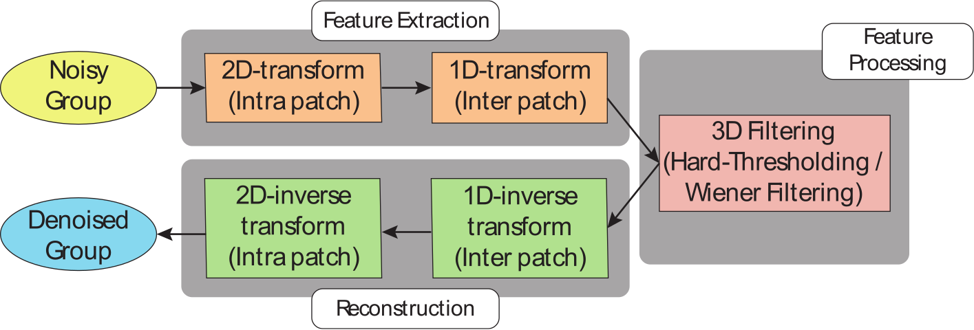
(a)

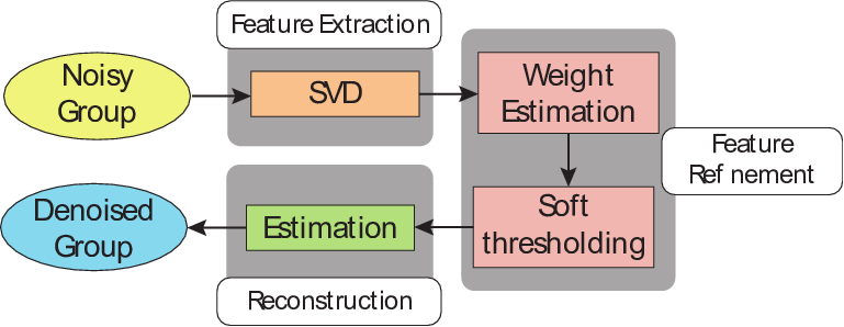
(b)

Figure 5: The group denoising schemes of (a) BM3D and (b) WNNM.

In BM3D, the input group is first projected to another domain by a 3D transformation. Specifically, they perform a 2D tranform to the patches followed by a 1D transform into the third dimension. Since the transform coefficients are often used as features in many image processing algorithms, the 3D transform corresponds to feature extraction stage. Also, as all the transformations employed in the BM3D (2D discrete cosine transform (DCT), 2D Bior transform and 1D Haar transform) are linear and the parameters are fixed, the entire 3D transform can be considered a convolution network with a single layer of large filter size. In many studies on deep neural network [38, 35], it has been shown that a convolution layer with large receptive field can be replaced by a series of small convolution layers. As a result, the feature extraction operator which involves a series of convolution can be viewed as a generalization of the 3D transform. After the transform, a 3D collaborative filtering is applied to the transformed group. Since the filtering attenuates the noise components from each coefficient, it corresponds to the feature refinement operation that maps noisy features to the denoised ones. The BM3D employs hard-thresholding and Wiener filtering for the refinement, where both are one-to-one non-linear mapping. In this sense, the collaborative filtering behaves as a special case of non-linear mapping with $1\times 1$ receptive field that can be implemented using neural network.

WNNM[7] transforms the matrix by singular value decomposition (SVD). The transformation can be viewed as a feature extraction operation that draws some features like basis or singluar value from the matrix. The SVD is relatively a complex operation compared to the multiplication by a constant matrix such as DCT or FFT. In an early work of the neural network [39], however, it has been explained that an optimal solution to an autoencoder is strongly related with the SVD. In other word, the SVD decomposition $[U,\Sigma,V]=SVD(\{Y_{p}\})$ and the reunion $\{\hat{X_{p}}\}=U\hat{\Sigma}V^{T}$ can be successfully replaced by the encoder and decoder of an autoencoder network. Therefore the proposed feature extraction and patch reconstruction operator can be considered a generalization of SVD. The singular values are refined by soft-thresholding whose weights are determined from the singular value itself. Therefore, as a 3D filtering in BM3D, the soft thresholding with the weight estimation behaves as a special case of one-to-one non-linear mapping.

In summary, our BMCNN and many NSS based methods follow the same process, i.e., block matching followed by feature extraction and processing in a certain domain by non-linear mappings. However, unlike manually deciding the parameters and non-linear mapping in the existing methods, the proposed BMCNN learns the corresponding procedures in a data-driven manner. It enables finding the optimal or at least suboptimal processing beyond the human design. Furthermore, the BMCNN trains an end-to-end mapping that consists of all operations rather than considering the operations separately.

IV Experiments

IV-A Training Methodology

The proposed denoising network is implemented using the Caffe package [40]. Training a network is identical to finding an optimal mapping function

$$\hat{x}_{p}=F(\{W_{i}\},y_{p})$$ (7)

where $W_{i}$ is the weight matrix including the bias for the $i$-th layer. This is achieved by minimizing a cost function

$$L(\{W_{i}\})=\frac{1}{N_{sample}}\sum{d(\hat{x}_{p},x_{p})}+\lambda r(\{W_{i}\})$$ (8)

where $N_{sample}$ is the total number of the training samples, $d(\hat{x}_{p},x_{p})$ is the distance between the estimated result $\hat{x}_{p}$ and its ground truth $x_{p}$, $r(\{W_{i}\})$ is a regularization term designed to enforce the sparseness, and $\lambda$ is the weight for the regularization term. Zhao et al[41] proposed several loss functions for neural networks, among which we employ the L1 norm for the distance:

$$d(\hat{x}_{p},x_{p})=\sum_{k}{\left|\hat{x}_{p}[k]-x_{p}[k]\right|}$$ (9)

because of its simplicity for implementation in addition to its promising performance for image restoration. The objective function is minimized using Adam, which is known as an efficient stochastic optimization method [42]. In detail, Adam solver updates $(W)_{i}$ by the formula

$$(m_{t})_{i} = \beta_{1}(m_{t-1})_{i}+(1-\beta_{1})(\bigtriangledown L(W_{t}))_{i},$$ (10)

$$(v_{t})_{i} = \beta_{1}(v_{t-1})_{i}+(1-\beta_{1})(\bigtriangledown L(W_{t}))^{2}_{i},$$ (11)

$$(W_{t+1})_{i} = (W_{t})_{i}-\alpha\frac{\sqrt{1-(\beta_{2})^{t}}}{1-(\beta_{1})^{t}}\frac{(m_{t})_{i}}{\sqrt{(v_{t})_{i}}+\epsilon}$$ (12)

where $\beta_{1}$ and $\beta_{2}$ are training parameters, $\alpha$ is the learning rate, and $\epsilon$ is a term to avoid zero division. In the proposed algorithm, the parameters are set as: $\lambda=0.0002,\alpha=0.001,\beta_{1}=0.9,\beta_{2}=0.999$ and $\epsilon=1e-8$. The initial values of $(W_{0})_{i}$ are set by Xavier initialization [43]. In Caffe, the Xavier initialization draws the values from the distribution

$$(W_{0})_{i}\sim N\left(0,\frac{1}{(N_{in})_{i}}\right)$$ (13)

where $(N_{in})_{i}$ is the number of neurons feeding into the layer. The bias of every convolution layer is initialized to a constant value 0.2. We train the BMCNN models for three noise levels: $\sigma=15,25$ and $50$.

IV-B Training and Test Data

Recent studies [18, 19] show that less than million training samples are sufficient to learn a favorable network. Following these works, we use 400 images from the Berkeley Segmentation dataset (BSDS) [44] for the training. All the images are cropped to the size of $180\times 180$ and data augmentation techniques like flip and rotation are applied. From all the images, training samples are extracted by the procedure in Sec. III-A. We set the block size as $20\times 20\times 4$ and the stride as 20. The total number of the training samples is 259,200.

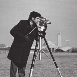
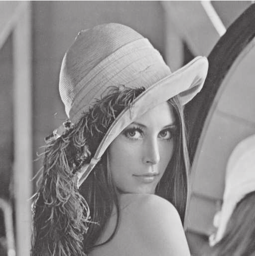
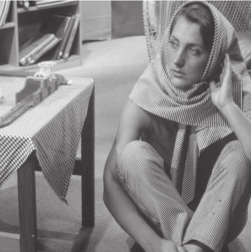
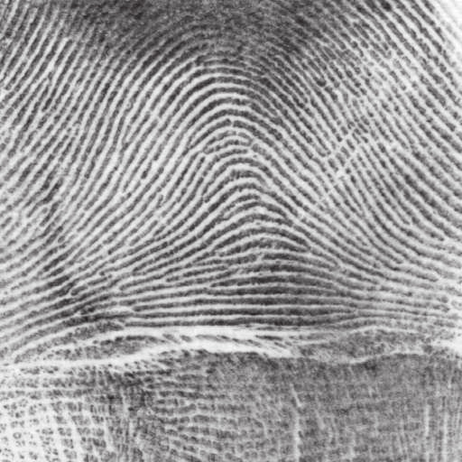
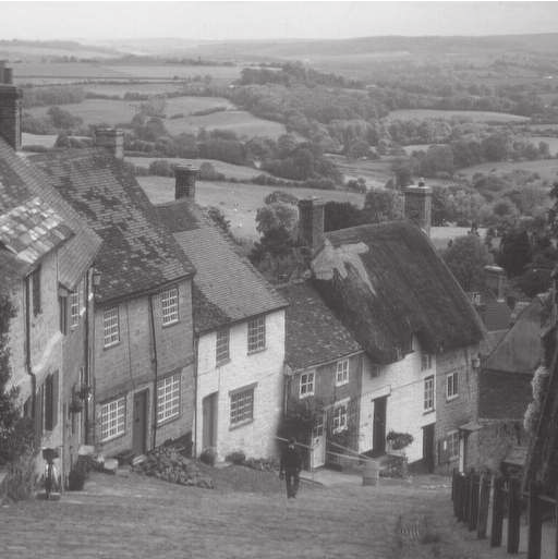
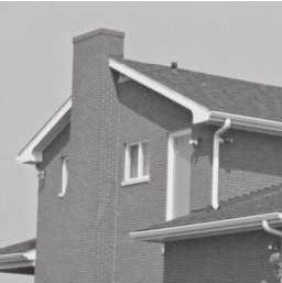
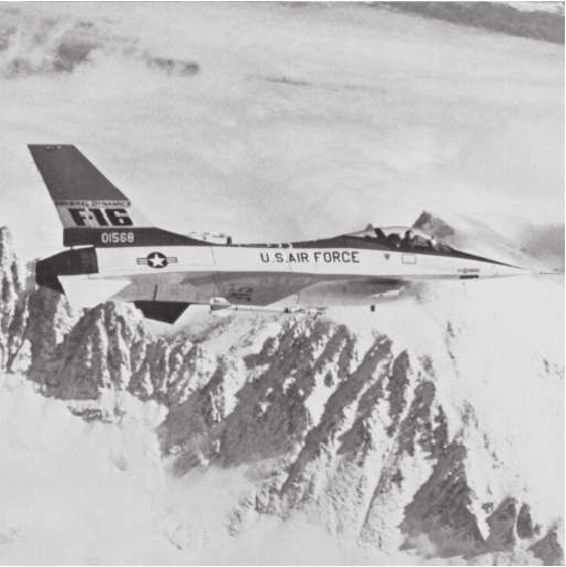
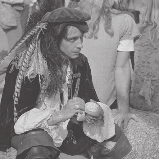
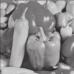
Figure 6: The 12 test images used in the experiments

We test our algorithm on standard images that are widely used for the test of denoising. Fig. 6 shows the 12 images that constitute the test set. The set contains 4 images of size $256\times 256$ (Cameraman, House, Peppers and Montage), and 8 images of size $512\times 512$ (Lena, Barbara, Boat, Fingerprint, Man, Couple, Hill and Jetplane). Note that the test set contains both repetitive patterns and irregularly textured images.

IV-C Comparision with the State-of-the-Art Methods

In this section, we evaluate the performance of the proposed BMCNN and compare it with the state-of-the-art denoising methods, including NSS based methods (BM3D [3], NCSR[4], and WNNM[7]) and training based methods (MLP [2], TNRD[18], and DnCNN[19]). All the experiments are performed on the same machine - Intel 3.4GHz dual core processor, nVidia GTX 780ti GPU and 16GB memory. The testing code for the proposed BMCNN is available at http://ispl.snu.ac.kr/clannad/BMCNN

IV-C1 Quantitave and Qualitative Evaluation

The PSNRs of denoised images are listed in Table I. It can be seen that the proposed BMCNN yields the highest average PSNR for every noise level. It shows that the PSNR is improved by 0.1$\sim$0.2dB compared to DnCNN. Especially, there are large performance gains in the case of images with regular and repetitive structure, such as Barbara and Fingerprint, which are the images that the NSS based methods perform better than the learning based methods. In this sense, it is believed that adopting the patch aggregation brings the cons of NSS to the learning based metod. Figs. 7 and 8 illustrate the visual results. The NSS based methods tend to blur the complex parts like a stalk of a fruit and the learning based methods often miss details on the repetitive parts such as the stripes of fingerprint. In contrast, the BMCNN recovers clear texture in both types of regions.

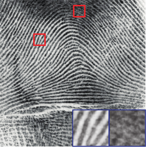
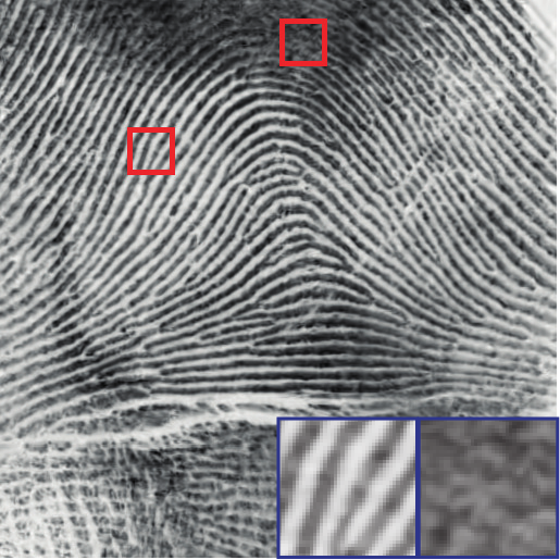
(a) Original	(b) BM3D	(c) NCSR	(d) WNNM
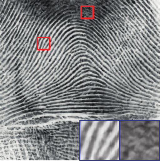
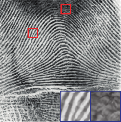
(e) MLP	(f) TNRD	(g) DnCNN	(h) BMCNN

Figure 7: Denoising result of the Fingerprint image with $\sigma$ = 25.

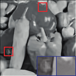
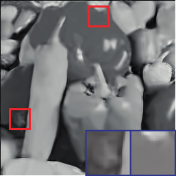
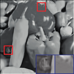
(a) Original	(b) BM3D	(c) NCSR	(d) WNNM
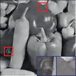
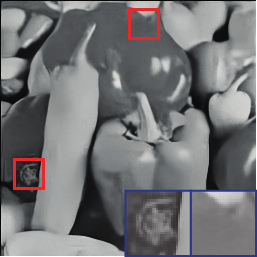
(e) MLP	(f) TNRD	(g) DnCNN	(h) BMCNN

Figure 8: Denoising result of the Peppers image with $\sigma$ = 50.

TABLE I: PSNR of different denoising methods. The best results are highlighted in bold.

Method	BM3D	NCSR	WNNM	MLP	TNRD	DnCNN	BMCNN
$\sigma=15$
Cameraman	31.91	32.01	32.17	-	32.18	32.61	32.73
Lena	34.22	34.11	34.35	-	34.23	34.59	34.61
Barbara	33.07	33.03	33.56	-	32.11	32.60	33.08
Boat	32.12	32.04	32.25	-	32.14	32.41	32.42
Couple	32.08	31.94	32.13	-	31.89	32.40	32.41
Fingerprint	30.30	30.45	30.56	-	30.14	30.39	30.41
Hill	31.87	31.90	32.00	-	31.89	32.13	32.08
House	35.01	35.04	35.19	-	34.63	35.11	35.16
Jetplane	34.09	34.11	34.38	-	34.28	34.55	34.53
Man	31.88	31.92	32.07	-	32.18	32.42	32.39
Montage	35.11	34.89	35.65	-	35.02	35.52	35.97
Peppers	32.68	32.65	32.93	-	32.96	33.21	33.32
Average	32.86	32.84	33.10	-	32.82	33.16	33.26
$\sigma=25$
Cameraman	29.44	29.47	29.64	29.59	29.69	30.11	30.20
Lena	32.06	31.95	32.27	32.28	32.05	32.48	32.53
Barbara	30.64	30.57	31.16	29.51	29.33	29.94	30.58
Boat	29.86	29.68	30.00	29.94	29.89	30.21	30.25
Couple	29.69	29.46	29.78	29.72	29.69	30.10	30.12
Fingerprint	27.71	27.84	27.96	27.66	27.33	27.64	28.01
Hill	29.82	29.68	29.96	29.83	29.77	29.99	30.00
House	32.95	32.98	33.33	32.66	32.64	33.23	33.32
Jetplane	31.63	31.62	31.89	31.87	31.77	32.06	32.17
Man	29.56	29.56	29.73	29.83	29.81	30.06	30.06
Montage	32.34	31.84	32.47	32.09	32.27	32.97	33.47
Peppers	30.21	29.96	30.45	30.45	30.51	30.80	30.93
Average	30.49	30.38	30.72	30.44	30.39	30.80	30.97
$\sigma=50$
Cameraman	26.18	26.15	26.47	26.37	26.56	26.99	27.02
Lena	29.05	28.97	29.32	29.28	28.94	29.42	29.56
Barbara	27.08	26.93	27.70	25.26	25.69	26.13	26.84
Boat	26.72	26.50	26.89	27.04	26.85	27.17	27.19
Couple	26.42	26.19	26.59	26.68	26.48	26.88	26.91
Fingerprint	24.55	24.52	24.79	24.21	23.70	24.14	24.65
Hill	27.05	26.87	27.12	27.37	27.11	27.31	27.33
House	29.70	29.69	30.25	29.82	29.40	30.08	30.25
Jetplane	28.31	28.23	28.61	28.56	28.43	28.74	28.88
Man	26.73	26.62	26.91	27.05	26.94	27.18	27.17
Montage	27.65	27.62	27.97	28.06	28.12	29.03	29.50
Peppers	26.69	26.64	26.97	26.71	27.05	27.30	27.45
Average	27.18	27.08	27.47	27.20	27.11	27.53	27.73

IV-C2 Running Time

Table II shows the average run-time of the denoising methods for the images of sizes $256\times 256$ and $512\times 512$. For TNRD, DnCNN and BMCNN, the times on GPU are computed. As shown, many conventional NSS based methods need very long times, which is mainly due to the complex optimization and/or matrix decomposition. On the other hand, since the BM3D consists of simple linear transform and non-linear filtering, it is much faster than the NCSR and WNNM. Since our BMCNN also consists of convolution and simple ReLU function, its computational cost is also less than the WNNM and NCSR. The BMCNN is, however, slower than other learning based approaches for three main reasons. First, our algorithm is a two-step approach that uses another end-to-end denoising algorithm as a preprocessing step. Therefore the computational cost is doubled. Second, the BMCNN contains a block matching step, which is difficult to be implement with GPU. In our algorithm, the block matching step takes almost half of the run-time. Finally, because of the nature of block-matching, the BMCNN is inherently a patch-based denoising algorithm. In order to prevent the artifacts around the boundaries between the denoised patches, the patches are extracted with overlapping. Hence, a pixel is processed multiple times and the overall run-time increases. Although our algorithm is slower for these reasons, our BMCNN is still competitive considering that it is much faster than the conventional NSS based methods and that it provides higher PSNR than others.

TABLE II: Run time (in seconds) of various denoising methods of size $256\times 256$ with $\sigma=25$.

Methods	BM3D	NCSR	WNNM	MLP	TNRD	DnCNN	BMCNN
$256\times 256$	0.87	190.3	179.9	2.238	0.038	0.053	2.135
$512\times 512$	3.77	847.9	778.1	7.797	0.134	0.203	8.030

IV-D Effects of Network Formulation

In this subsection, we modify some settings of the BMCNN to investigate the relations between the settings and performance. All the additional experiments are made with $\sigma=25$.

TABLE III: PSNR results of BMCNN, woBMCNN and their base preprocessing-DnCNN.

	BMCNN	woBMCNN	DnCNN
Cameraman	30.20	30.08	30.11
Lena	32.53	32.45	32.48
Barbara	30.58	29.91	29.94
Boat	30.25	30.17	30.21
Couple	30.12	30.09	30.10
Fingerprint	28.01	27.61	27.64
Hill	30.00	29.96	29.99
House	33.32	33.20	33.23
Jetplane	32.17	32.02	32.06
Man	30.06	30.04	30.06
Montage	33.47	33.02	32.97
Peppers	30.93	30.81	30.80
Average	30.97	30.78	30.80

IV-D1 NSS Prior

In this paper, we take the NSS prior into account by adopting block matching, i.e., by using the aggregated similar patches as the input to the CNN. In order to show the effect of NSS prior, we conduct an additional experiment: we train a network that estimates a denoised patch using only two patches as the input, specifically a noisy patch and corresponding pilot patch without further aggregation. We name the network as woBMCNN, and its PSNR results are summarized in Table. III. The result validates that the performance gain is owing to the block matching rather than two-step denoising. Interestingly, the woBMCNN does not perform better than DnCNN, which is used as the preprocessing. Actually, the woBMCNN can be interpreted as a deeper network with similar network formulation and a skip connection [45]. However, since the DnCNN is already a favorable network and the performance with the formulation is saturated, the deeper network can hardly perform better. On the other hands, the BMCNN encodes additional information to the network, which is shown to play an important role.

TABLE IV: PSNR results of BMCNN with various patch sizes.

	$10\times 10$	$20\times 20$	$40\times 40$
Cameraman	28.82	30.20	30.00
Lena	30.42	32.53	32.39
Barbara	29.05	30.58	29.72
Boat	29.01	30.25	30.07
Couple	28.89	30.12	29.97
Fingerprint	27.24	28.01	27.51
Hill	28.83	30.00	29.89
House	30.85	33.32	33.11
Jetplane	30.20	32.17	31.96
Man	28.84	30.06	29.96
Montage	30.47	33.47	32.72
Peppers	29.31	30.93	30.67
Average	29.33	30.97	30.66

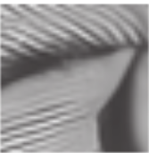
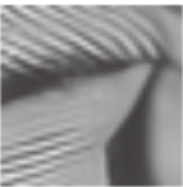
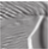
(a) $10\times 10$	(b) $20\times 20$	(c) $40\times 40$
Error : 0.0515	Error : 0.0672	Error : 0.1813

Figure 9: The illustration of block matching results for various patch sizes. The first row shows reference patches, the second row shows the 3rd-similar patches to the references and the third row shows the difference of the first and the second row. The error is defined as the average value of the difference.

IV-D2 Patch Size

In many patch-based algorithms, the patch size is an important parameter that affects the performance. We train three networks with patch size $10\times 10$, $20\times 20$ (base) and $40\times 40$. Table IV shows that $20\times 20$ patch works better than other sizes. Moreover, networks of patch size $10\times 10$ and $40\times 40$ work even worse than its preprocessing.

Burger et al. [2] revealed that a larger patch contains more information, and thus the neural network can learn more accurate objective function with larger training patches. On the contrary, we cannot train the mapping function reasonably with small patches. But the large patch degrades the block matching performance, because it becomes more difficult to find well matched patches as the patch size increases. Fig. 9 shows the block matching result and the error for various patch sizes. For a $10\times 10$ patch and a $20\times 20$ patch, the block-matching finds almost the same patches and the error is very small. For a $40\times 40$ patch, on the other hands, decent portion of the patch does not fit well and the error becomes so big. Conventional NSS based algorithms including [3] and [5] also prefer small patches whose sizes are around $10\times 10$ for these reasons. To conclude, $20\times 20$ is the proper patch size that satisfies both CNN and NSS prior.

TABLE V: PSNR and run time results of BMCNN with various stride.

	5	10	15	20
Cameraman	30.21	30.20	30.20	30.18
Lena	32.53	32.53	32.52	32.51
Barbara	30.58	30.58	30.56	30.49
Boat	30.25	30.25	30.25	30.24
Couple	30.12	30.12	30.12	30.11
Fingerprint	28.03	28.01	28.01	27.97
Hill	30.00	30.00	30.00	30.00
House	33.32	33.32	33.32	33.30
Jetplane	32.17	32.17	32.16	32.16
Man	30.06	30.06	30.05	30.05
Montage	33.49	33.47	33.45	33.40
Peppers	30.94	30.93	30.93	30.92
Average PSNR	30.98	30.97	30.96	30.94
Average time($256\times 256$)	4.271	2.151	1.765	1.603
Average time($512\times 512$)	16.79	8.101	6.492	5.777

IV-D3 Stride

Since the proposed method is patch-based, its performance depends on the stride value to divide the input images into the patches. With a small stride, each pixel appears in many patches, which means that every pixel is processed multiple times. It definitely increases the computational costs but has the possiblity of performance improvement. We test our algorithm with various stride values and the results are summarized in the Table V. From the result, we determine that a stride value around the half of the patch size shows reasonable performance for both the run time and the PSNR.

TABLE VI: PSNR of BMCNN results with two different preprocessing.

	BMCNN-DnCNN	BMCNN-BM3D
Cameraman	30.20	30.03
Lena	32.53	32.49
Barbara	30.58	31.23
Boat	30.25	30.16
Couple	30.12	30.02
Fingerprint	28.02	28.06
Hill	30.00	30.05
House	33.32	33.43
Jetplane	32.17	32.14
Man	30.06	29.94
Montage	33.47	33.31
Peppers	30.93	30.78
Average	30.97	30.97

IV-D4 Pilot Signal

We also conduct an experiment to see how the different preprocessing methods (other than DnCNN in the previous experiments) affect the the overall performance. For the experiment, we employ BM3D [3] due to its NSS based nature and reasonable run time. Table VI shows the denoising performance with different preprocessing methods and two interesting characteristics can be found.

• The performance on the individual image depends on the preprocessing method. BMCNN-BM3D shows better performance on Barbara, Fingerprint and House, where NSS based WNNM performed better than the CNN based DnCNN.

• However, the overall performance shows negligible difference. It implies the overall performance of the denoising network depends on the network formulation, not the preprocessing.

V Conclusion

In this paper, we have proposed a framework that combines two dominant approaches in up-to-date image denoising algorithms, i.e., the NSS prior based methods and CNN based methods. We train a network that estimates a noise component from a group of similar patches. Unlike the conventional NSS based methods, our denoiser is trained in a data-driven manner to learn an optimal mapping function and thus achieves better performance. Our BMCNN also shows better performance than the existing CNN based method especially in the case of images with regular structure, because the BMCNN considers NSS in addition to the local characteristics.

References

- [1] A. Buades, B. Coll, and J.-M. Morel, “A non-local algorithm for image denoising,” in Proc. of Computer Vision and Pattern Recognition (CVPR), 2005, pp. 60–65.
- [2] H. C. Burger, C. J. Schuler, and S. Harmeling, “Image denoising: Can plain neural networks compete with bm3d?” in Proc. of Computer Vision and Pattern Recognition (CVPR), 2012, pp. 2392–2399.
- [3] K. Dabov, A. Foi, V. Katkovnik, and K. Egiazarian, “Image denoising by sparse 3-d transform-domain collaborative filtering,” IEEE Trans. Image process., vol. 16, no. 8, pp. 2080–2095, 2007.
- [4] W. Dong, L. Zhang, G. Shi, and X. Li, “Nonlocally centralized sparse representation for image restoration,” IEEE Trans. Image process., vol. 22, no. 4, pp. 1620–1630, 2013.
- [5] W. Dong, G. Shi, and X. Li, “Nonlocal image restoration with bilateral variance estimation: a low-rank approach,” IEEE Trans. Image process., vol. 22, no. 2, pp. 700–711, 2013.
- [6] A. Foi, V. Katkovnik, and K. Egiazarian, “Pointwise shape-adaptive dct for high-quality denoising and deblocking of grayscale and color images,” IEEE Trans. Image process., vol. 16, no. 5, pp. 1395–1411, 2007.
- [7] S. Gu, L. Zhang, W. Zuo, and X. Feng, “Weighted nuclear norm minimization with application to image denoising,” in Proc. of Computer Vision and Pattern Recognition (CVPR), 2014, pp. 2862–2869.
- [8] O. G. Guleryuz, “Weighted overcomplete denoising,” in Proc. of Asilomar Conference on Signals, Systems and Computer, 2003, pp. 1992–1996.
- [9] V. Jain and S. Seung, “Natural image denoising with convolutional networks,” in Advances in Neural Information Processing Systems (NIPS), 2009, pp. 769–776.
- [10] X. Jia, X. Feng, and W. Wang, “Adaptive regularizer learning for low rank approximation with application to image denoising,” in Proc. of International Conference on Image Processing (ICIP), 2016, pp. 3096–3100.
- [11] B. Wang, T. Lu, and Z. Xiong, “Adaptive boosting for image denoising: Beyond low-rank representation and sparse coding,” in Proc. of the International Conference on Pattern Recognition (ICPR), 2016.
- [12] S. J. You and N. I. Cho, “A new image denoising method based on the wavelet domain nonlocal means filtering,” in Proc. of International Conference on Acoustics, Speech and Signal Processing (ICASSP), 2011, pp. 1141–1144.
- [13] B. Jin, S. J. You, and N. I. Cho, “Bilateral image denoising in the laplacian subbands,” EURASIP Journal on Image and Video Processing, vol. 2015, no. 1, pp. 1–12, 2015.
- [14] J. Mairal, F. Bach, J. Ponce, G. Sapiro, and A. Zisserman, “Non-local sparse models for image restoration,” in Proc. of the International Conference on Computer Vision (ICCV), 2009, pp. 2272–2279.
- [15] M. Nejati, S. Samavi, S. R. Soroushmehr, and K. Najarian, “Low-rank regularized collaborative filtering for image denoising,” in Proc. of International Conference on Image Processing (ICIP), 2015, pp. 730–734.
- [16] Z. Zha, X. Liu, Z. Zhou, X. Huang, J. Shi, Z. Shang, L. Tang, Y. Bai, Q. Wnag, and X. Zhang, “Image denoising via group sparsity residual constraint,” in Proc. of International Conference on Acoustics, Speech and Signal Processing(ICASSP), 2017, pp. 1787–1791.
- [17] U. Schmidt and S. Roth, “Shrinkage fields for effective image restoration,” in Proc. of Computer Vision and Pattern Recognition (CVPR), 2014, pp. 2774–2781.
- [18] Y. Chen and T. Pock, “Trainable nonlinear reaction diffusion: A flexible framework for fast and effective image restoration,” IEEE Trans. Pattern Analysis and Machine Intelligence, 2016.
- [19] K. Zhang, W. Zuo, Y. Chen, D. Meng, and L. Zhang, “Beyond a gaussian denoiser: Residual learning of deep cnn for image denoising,” IEEE Trans. Image process., 2017.
- [20] H. C. Burger, C. Schuler, and S. Harmeling, “Learning how to combine internal and external denoising methods,” in Proc. of German Conference on Pattern Recognition, 2013, pp. 121–130.
- [21] M. Elad and M. Aharon, “Image denoising via sparse and redundant representations over learned dictionaries,” IEEE Trans. Image process., vol. 15, no. 12, pp. 3736–3745, 2006.
- [22] B. Recht, M. Fazel, and P. A. Parrilo, “Guaranteed minimum-rank solutions of linear matrix equations via nuclear norm minimization,” SIAM review, vol. 52, no. 3, pp. 471–501, 2010.
- [23] Y. LeCun, L. Bottou, Y. Bengio, and P. Haffner, “Gradient-based learning applied to document recognition,” Proc. IEEE, vol. 86, no. 11, pp. 2278–2324, 1998.
- [24] C. J. Schuler, H. Christopher Burger, S. Harmeling, and B. Scholkopf, “A machine learning approach for non-blind image deconvolution,” in Proc. of Computer Vision and Pattern Recognition (CVPR), 2013, pp. 1067–1074.
- [25] S. Geman and C. Graffigne, “Markov random field image models and their applications to computer vision,” in Proc. of the International Congress of Mathematicians, 1986, p. 2.
- [26] C. Dong, C. C. Loy, K. He, and X. Tang, “Learning a deep convolutional network for image super-resolution,” in Proc. of European Conference on Computer Vision (ECCV), 2014, pp. 184–199.
- [27] J. Yang, J. Wright, T. S. Huang, and Y. Ma, “Image super-resolution via sparse representation,” IEEE Trans. Image process., vol. 19, no. 11, pp. 2861–2873, 2010.
- [28] C. Dong, Y. Deng, C. Change Loy, and X. Tang, “Compression artifacts reduction by a deep convolutional network,” in Proc. of the International Conference on Computer Vision (ICCV), 2015, pp. 576–584.
- [29] J. Kim, J. K. Lee, and K. M. Lee, “Deeply-recursive convolutional network for image super-resolution,” in Proc. of Computer Vision and Pattern Recognition (CVPR), 2016, pp. 1637–1645.
- [30] ——, “Accurate image super-resolution using very deep convolutional networks,” in Proc. of Computer Vision and Pattern Recognition (CVPR), 2016, pp. 1646–1654.
- [31] Y. Bengio, P. Simard, and P. Frasconi, “Learning long-term dependencies with gradient descent is difficult,” IEEE Trans. Neural networks, vol. 5, no. 2, pp. 157–166, 1994.
- [32] K. He, X. Zhang, S. Ren, and J. Sun, “Deep residual learning for image recognition,” in Proc. of Computer Vision and Pattern Recognition (CVPR), 2016, pp. 770–778.
- [33] S. Ioffe and C. Szegedy, “Batch normalization: Accelerating deep network training by reducing internal covariate shift,” in Proc. of International Conference on Machine Learning (ICML), 2015, pp. 448–456.
- [34] R. Timofte, V. De Smet, and L. Van Gool, “A+: Adjusted anchored neighborhood regression for fast super-resolution,” in Proc. of Asian Conference on Computer Vision(ACCV), 2014, pp. 111–126.
- [35] K. Simonyan and A. Zisserman, “Very deep convolutional networks for large-scale image recognition,” arXiv preprint arXiv:1409.1556, 2014.
- [36] T. Salimans and D. P. Kingma, “Weight normalization: A simple reparameterization to accelerate training of deep neural networks,” in Advances in Neural Information Processing Systems(NIPS), 2016, pp. 901–901.
- [37] H. Noh, S. Hong, and B. Han, “Learning deconvolution network for semantic segmentation,” in Proc. of the International Conference on Computer Vision(ICCV), 2015, pp. 1520–1528.
- [38] C. Szegedy, W. Liu, Y. Jia, P. Sermanet, S. Reed, D. Anguelov, D. Erhan, V. Vanhoucke, and A. Rabinovich, “Going deeper with convolutions,” in Proc. of Computer Vision and Pattern Recognition (CVPR), 2015, pp. 1–9.
- [39] H. Bourlard and Y. Kamp, “Auto-association by multilayer perceptrons and singular value decomposition,” Biological cybernetics, vol. 59, no. 4-5, pp. 291–294, 1988.
- [40] Y. Jia, E. Shelhamer, J. Donahue, S. Karayev, J. Long, R. Girshick, S. Guadarrama, and T. Darrell, “Caffe: Convolutional architecture for fast feature embedding,” in Proc. of the ACM international conference on Multimedia (ACM MM), 2014, pp. 675–678.
- [41] H. Zhao, O. Gallo, I. Frosio, and J. Kautz, “Loss functions for image restoration with neural networks,” IEEE Trans. Computational Imaging, 2016.
- [42] D. Kingma and J. Ba, “Adam: A method for stochastic optimization,” in International Conference for Learning Representations, 2015.
- [43] X. Glorot and Y. Bengio, “Understanding the difficulty of training deep feedforward neural networks.” in Aistats, vol. 9, 2010, pp. 249–256.
- [44] P. Arbelaez, C. Fowlkes, and D. Martin, “The berkeley segmentation dataset and benchmark,” http://www.eecs.berkeley.edu/Research/Projects/CS/vision/bsds, 2007.
- [45] X. Mao, C. Shen, and Y.-B. Yang, “Image restoration using very deep convolutional encoder-decoder networks with symmetric skip connections,” in Advances in Neural Information Processing Systems(NIPS), 2016, pp. 2802–2810.