UPGMA and the normalized equidistant minimum evolution problem

Abstract

UPGMA (Unweighted Pair Group Method with Arithmetic Mean) is a widely used clustering method. Here we show that UPGMA is a greedy heuristic for the normalized equidistant minimum evolution (NEME) problem, that is, finding a rooted tree that minimizes the minimum evolution score relative to the dissimilarity matrix among all rooted trees with the same leaf-set in which all leaves have the same distance to the root. We prove that the NEME problem is NP-hard. In addition, we present some heuristic and approximation algorithms for solving the NEME problem, including a polynomial time algorithm that yields a binary, rooted tree whose NEME score is within $O(\log^{2}n)$ of the optimum. We expect that these results to eventually provide further insights into the behavior of the UPGMA algorithm.

1 Introduction

Clustering (i.e. subdividing a dataset into smaller subgroups or clusters) is a fundamental task in data analysis, and has a wide range of applications (see, e.g. [1]). An important family of clustering methods aim to produce a clustering of a dataset in which the clusters form a hierarchy where the clusters nest within one another. Such hierarchies are typically represented by leaf-labeled tree structures known as dendrograms or rooted phylogenetic trees. Introduced in 1958 [2], average linkage analysis, usually referred to as UPGMA (Unweighted Pair Group Method with Arithmetic Mean), is arguably the most popular hierarchical clustering algorithm in use to date, and remains widely cited and extremely popular (see, e.g. [3]). This is probably because UPGMA is conceptually easy to understand and fast in practice, an important consideration as big data sets are becoming the norm in many areas. UPGMA is commonly used in phylogenetics and taxonomy to build evolutionary trees [4, Chapter 11] as well as in related areas such as ecology [5] and metagenomics [6]. In addition, it is used as a general hierarchical clustering tool in bioinformatics and other areas including data mining and pattern recognition [7, Chapter 2].

UPGMA is a text-book algorithm that belongs to the family of agglomerative clustering methods that share the following common bottom-up scheme (cf. e.g. [4, p.162]). They take as input a dissimilarity $D$ on a set $X$, i.e. a real-valued, symmetric map on $X\times X$ which vanishes on the diagonal, and build a collection of clusters or subsets of $X$ which correspond to a rooted tree with leaf-set $X$. To do this, at each step two clusters with the minimum inter-cluster dissimilarity are combined to create a new cluster, starting with the collection of clusters consisting of singleton subsets of $X$, and finishing when the cluster $X$ is obtained. Different formulations of the inter-cluster dissimilarity, which specifies the dissimilarity of sets as a function of the dissimilarities observed on the members of the sets, lead to different heuristic criteria of the agglomerative methods. UPGMA, as the name average linkage analysis suggests, uses the mean dissimilarity across all pairs of elements that are contained within the two clusters. Formally, two clusters $A,B\subseteq X$ are selected for merging at each iteration step of UPGMA if the average

$$\frac{1}{|A||B|}\sum_{a\in A,\,b\in B}D(a,b)$$

is minimized over all possible pairs of clusters. Since the arithmetic mean is used, UPGMA is often more stable than linkage methods in which only a subset of the elements within the clusters are used (e.g. the single-linkage method).

UPGMA is commonly thought of as a method that greedily constructs a rooted phylogenetic tree that is closest to the input dissimilarity matrix in the least squares sense [8]. However, it is not guaranteed to do so, although it often does quite well in practice [4, p.162]. In [9] it was shown that the related Neighbor-Joining [10] method for constructing unrooted phylogenetic trees from dissimilarity matrices can be thought of as a greedy heuristic that minimizes the so-called balanced minimum evolution score. Here we shall observe that (see Section 3), completely analogously, UPGMA is a greedy heuristic for computing a rooted phylogenetic tree that minimizes the so-called minimum evolution score [11] over all rooted phylogenetic trees on the same fixed leaf-set in which all leaves have the same distance in the tree to the root. We refer to this optimization problem as the normalized equidistant minimum evolution (NEME) problem, and expect that a better understanding of this problem will provide further insights into the behavior of the UPGMA algorithm.

1.1 Related work

Theoretical properties of discrete optimization problems arising in the construction of evolutionary trees have been studied for many years (for some earlier work see, e.g. [12, 13, 14]). Among these, the problems falling under the name of minimum evolution alone form a quite diverse family (see, e.g. [15]), in which the so-called balanced minimum evolution problem [16] is a particularly well-studied member. For this problem it was recently shown in [17] that for general $n\times n$-input dissimilarity matrices there exists a constant $c>1$ such that no polynomial time algorithm can achieve an approximation factor of $c^{n}$ unless P equals NP. We note that this hardness result does not rely on the often imposed restriction (see, e.g. [18, 13]) that the edge lengths of the constructed tree must be integers. Moreover, in contrast to general input dissimilarity matrices, for inputs that are metrics (i.e. matrices that also satisfy the triangle inequality) a polynomial time algorithm with an approximation factor of $2$ is presented in [17]. Interestingly, the proof of this approximation factor uses the fact that the balanced minimum evolution score of an unrooted tree can be interpreted as being the average length of a spanning cycle compatible with the structure of the tree [19].

Another recent, related direction of work considers the algebraic structure of the space of rooted phylogenetic trees induced by the UPGMA method (see, e.g. [8, 20]). This algebraic structure is tightly linked with the property of consistency of a tree construction method, that is, those conditions under which the method is able to reconstruct a tree that has been used to generate the input dissimilarity matrix (see, e.g. [21]). In the context of our work, we are particularly interested in the consistency of methods that perform a local search of the space of all rooted phylogenetic trees on a fixed set of leaves (see, e.g. [16]). Again, balanced minimum evolution is the variant of minimum evolution for which some consistency results of this type are known [22, 23].

1.2 Our results and organization

After presenting some preliminaries in the next section, in Section 3 we begin by giving an explicit formula of the minimum evolution score of a rooted tree $T$ as a linear combination of the input dissimilarities. This formula allows us to interpret the minimum evolution score of $T$ in terms of the average length of a minimum spanning tree compatible with the set of clusters induced by $T$.

Using this observation, we explain how UPGMA can be regarded as a greedy heuristic for the NEME problem. In addition, we show that there are rooted phylogenetic trees with $n$ leaves on which some input dissimilarity matrix has an optimal least squares fit while the NEME score of that tree for the same dissimilarity matrix is worse than the minimum NEME score by a factor in $\Omega(n^{2})$. This highlights the fact that the NEME problem and searching for trees with minimum least squares fit are quite distinct problems.

Next, in Section 4, we explore solving the NEME problem by performing a local search of the space of binary rooted phylogenetic trees using so-called rooted nearest neighbor interchanges as the moves in the local search. We show that this approach is consistent. More specifically, for any input dissimilarity matrix that can be perfectly represented by a unique binary rooted phylogenetic tree with all leaves having the same distance from the root, we prove that the local search will arrive at this tree after a finite number of moves.

In Section 5 we show that the NEME problem is NP-hard even for $n\times n$ input distance matrices that satisfy the triangle inequality and only take on $O(\log n)$ different values. In light of this fact, in Section 6 we consider some approximation algorithms for solving the NEME problem. More specifically, we first show that the tree produced by UPGMA can have a score that is worse than the minimum score by a factor in $\Omega(n)$. Then, for dissimilarity matrices that satisfy the triangle inequality, we present a polynomial time algorithm that yields a binary rooted phylogenetic tree whose NEME score is within $O(\log^{2}n)$ of the optimum. We conclude in Section 7 by mentioning two possible directions for future work.

2 Preliminaries

In this section we give a formal definition of the NEME problem and introduce some of the notation and terminology that will be used throughout this paper.

Let $X$ be a finite non-empty set. A dissimilarity on $X$ is a symmetric map $D:X\times X\rightarrow\mathbb{R}$ with $D(x,x)=0$ for all $x\in X$. In this paper, a rooted phylogenetic tree on $X$ is a rooted tree $T=(V,E,\rho)$ with (i) root $\rho$ of degree 1, (ii) leaf set $X$ and (iii) every vertex not in $X\cup\{\rho\}$ having degree at least 3. Note that even though we require the root to have degree 1, we do not consider it a leaf of the tree. A normalized equidistant edge weighting (NEEW) of a rooted phylogenetic tree $T=(V,E,\rho)$ on $X$ is a map $\omega:E\rightarrow\mathbb{R}$ such that the total weight of the edges on the path from $\rho$ to $x$ is 0 for all $x\in X$. More generally, for all $u,v\in V$, we denote the total weight of the edges on the path between vertices $u$ and $v$ by $\ell_{(T,\omega)}(u,v)$. The height $h_{(T,\omega)}(v)$ of any vertex $v\in V$ is defined as $\ell_{(T,\omega)}(v,x)$ for any leaf $x$ in the subtree of $T$ rooted at $v$. The length $\ell_{\omega}(T)$ of $T$ under the edge weighting $\omega$ is $\sum_{e\in E}\omega(e)$, that is, the total weight of all edges of $T$.

Note that the length of any rooted phylogenetic tree $T=(V,E,\rho)$ on $X$ with a normalized equidistant edge weighting $\omega$ can also be expressed as follows:

$$\ell_{\omega}(T)=\sum_{v\in(V-(X\cup\{\rho\}))}(deg(v)-2)\cdot h_{(T,\omega)}(v),$$ (1)

where $deg(v)$ denotes the degree of vertex $v$ in $T$. Note that the restriction of $\ell_{(T,\omega)}$ to $X\times X$ yields a dissimilarity $D_{(T,\omega)}$ on $X$. Moreover, this dissimilarity is an ultrametric, that is, $D_{(T,\omega)}(x,z)\leq\max\{D_{(T,\omega)}(x,y),D_{(T,\omega)}(y,z)\}$ holds for all $x,y,z\in X$, if and only if the edge weighting $\omega$ assigns a non-negative real number to each edge not adjacent to a vertex in $X\cup\{\rho\}$. We call any such edge weighting interior positive.

Let $D$ be a dissimilarity on $X$ and $T=(V,E,\rho)$ a rooted phylogenetic tree on $X$. For any vertex $v\in V$ let $ch(v)$ denote the set of children of $v$, that is, the set of vertices $u$ that are adjacent to $v$ and for which $v$ lies on the path from $u$ to $\rho$. Moreover, we refer to $v$ as the parent of the vertices $u\in ch(v)$ and we denote by $C(v)$ the cluster of elements in $X$ induced by $v$, that is, the set of those leaves $x$ of $T$ for which the path from $x$ to $\rho$ contains $v$. In [24] it is shown that, for any dissimilarity $D$ and any rooted phylogenetic tree $T$ on $X$, there is a unique normalized equidistant edge weighting $\omega=\omega_{(D,T)}$ with

$$\Delta(D,D_{(T,\omega)})=\sum_{\{x,y\}\in\binom{X}{2}}\big{(}D(x,y)-D_{(T,\omega)}(x,y)\big{)}^{2}$$

minimum, where $\binom{X}{2}$ denotes the set of 2-element subsets of $X$. More precisely, this edge weighting is the unique solution of the system of linear equations

$$\ell_{(T,\omega)}(v,y)$$

$$=\frac{1}{2\sum_{\{u,u^{\prime}\}\in\binom{ch(v)}{2}}|C(u)|\cdot|C(u^{\prime})|}\sum_{\{u,u^{\prime}\}\in\binom{ch(v)}{2}}\sum_{\begin{subarray}{c}x\in C(u)\\ x^{\prime}\in C(u^{\prime})\end{subarray}}D(x,x^{\prime}),$$ (2)

for all $v\in V-(X\cup\{\rho\})$, and $\ell_{(T,\omega)}(v,y)=0$, for all $v\in X\cup\{\rho\}$, $y\in C(v)$. Note that this is the analogue to Vach’s theorem for unrooted trees [25]. For later use, we put $\Delta(D,D_{(T,\omega_{(D,T)})})=\Delta(D,T)$.

Now, the normalized equidistant minimum evolution score of a rooted phylogenetic tree $T$ on $X$ with respect to a dissimilarity $D$ on $X$ is formally defined as

$$\sigma_{D}(T)=\ell_{\omega_{(D,T)}}(T),$$

that is, the length of $T$ under the edge weighting $\omega_{(D,T)}$. The NEME problem is to compute, for an input dissimilarity $D$ on $X$, a rooted phylogenetic tree on $X$ with minimum NEME score. Formally, it can be stated as below.

Problem NEME Problem
Instance: A distance matrix $D$ on a finite set $X$ and a number $p$.
Question: Does there exist a rooted phylogenetic tree $T$ on $X$ such that $\sigma_{D}(T)\leq p$ holds.

3 UPGMA and the NEME problem

We begin this section by explaining how the UPGMA algorithm can be reinterpreted as a greedy approach to solving the NEME problem. First note that it follows directly from Equations (1) and (2) that the NEME score of a rooted phylogenetic tree $T=(V,E,\rho)$ can be written as the following linear combination of the given dissimilarity values:

$$\sigma_{D}(T) =\sum_{\{x,y\}\in\binom{X}{2}}\alpha_{\{x,y\}}^{T}\cdot D(x,y)\quad\text{with}$$ (3)

$$\alpha_{\{x,y\}}^{T} =\frac{deg(lca(x,y))-2}{2\sum_{\{u,u^{\prime}\}\in\binom{ch(lca(x,y))}{2}}|C(u)|\cdot|C(u^{\prime})|},$$

where $lca(u,v)$ is the lowest common ancestor in $T$ for any two vertices $u,v\in V$. In particular, in case $T$ is a binary tree, that is, every vertex not in $X\cup\{\rho\}$ has degree precisely 3, we obtain, for any $\{x,y\}\in\binom{X}{2}$ the coefficient

$$\alpha_{\{x,y\}}^{T}=\frac{1}{2\prod_{u\in ch(lca(x,y))}|C(u)|}.$$ (4)

As an immediate consequence of (3) we obtain that the score $\sigma_{D}(T)$ is linear in $D$, that is, when $D$ can be written as $D=\lambda_{1}\cdot D_{1}+\lambda_{2}\cdot D_{2}$ for non-negative real numbers $\lambda_{i}$ and dissimilarities $D_{i}$, $i\in\{1,2\}$, then

$$\sigma_{D}(T)=\lambda_{1}\cdot\sigma_{D_{1}}(T)+\lambda_{2}\cdot\sigma_{D_{2}}(T)$$ (5)

To link the Formula (3) with the UPGMA algorithm, recall that this algorithm constructs a rooted phylogenetic tree by generating the list of clusters associated to the vertices of this tree. It starts with the singleton clusters associated to the leaves of the tree. Then, in each iteration of the algorithm we already have a partition $\mathcal{C}=\{C_{1},C_{2},\dots,C_{m}\}$ of $X$ into $m\geq 2$ clusters and a dissimilarity $D$ on $X$. UPGMA then selects a pair of two distinct clusters $A,B\in\mathcal{C}$ that minimizes

$$\frac{1}{|A||B|}\sum_{a\in A,\,b\in B}D(a,b)$$

and returns the partition $(\mathcal{C}-\{A,B\})\cup\{A\cup B\}$. Now it is easy to see that UPGMA in each iteration greedily pairs already selected clusters so as to locally minimize the value added to the score $\sigma_{D}(T)$ for the rooted phylogenetic tree $T$ produced by the method.

Interestingly, the coefficients in (4) suggest the following alternative interpretation of the NEME score of a binary rooted phylogenetic tree $T=(V,E,\rho)$: Consider the complete graph $G$ with vertex set $X$. Each edge $\{x,y\}$ of $G$ is weighted with the value $D(x,y)$. We construct a random subgraph of $G$ as follows. For each vertex $v\in V-(X\cup\{\rho\})$ select a random edge that has precisely one end point in each cluster associated with the two children of $v$. Let $H$ denote the resulting subgraph of $G$. It is easy to see that $H$ is always a spanning tree of $G$. Thus, in case $T$ is binary, $\sigma_{D}(T)$ can be interpreted as half the average length of a random spanning tree $H$ of $G$ that is compatible with the clusters of $T$. Based on (3), this interpretation can be extended to the non-binary case where, instead of a spanning tree, a random spanning forest in $G$ with $|X|-1$ edges, some of which selected more than once, arises.

Next we present a technical lemma summarizing some simple observations about the NEME score that will be used later. Let ${\bf R}_{X}$ denote the set of all rooted phylogenetic trees on $X$. In addition let ${\bf BR}_{X}$ denote the subset of those trees in ${\bf R}_{X}$ that are binary.

Lemma 1

Let $D$ be a non-negative dissimilarity on a finite set $X$ with $|X|=n\geq 2$. Then, for all $T\in{\bf R}_{X}$, we have:

• $$\sum_{\{x,y\}\in\binom{X}{2}}\alpha_{\{x,y\}}^{T}=\frac{1}{2}(n-1),$$

• $$\frac{2}{n^{2}}\leq\min\{\alpha_{\{x,y\}}^{T}:\{x,y\}\in\binom{X}{2}\}\leq\max\{\alpha_{\{x,y\}}^{T}:\{x,y\}\in\binom{X}{2}\}\leq\frac{1}{2},$$

• $$\sigma_{D}(T)\leq\frac{n^{2}}{4}\min\{\sigma_{D}(T^{\prime}):T^{\prime}\in{\bf R}_{X}\}.$$

Proof. (i): We use induction on $n$. For $n=2$ the equality clearly holds. Next assume $n\geq 3$ and consider any $T\in{\bf R}_{X}$. Let $u$ be the single child of $\rho$. Put $k=deg(u)-1$ and let $v_{1},v_{2},\dots,v_{k}$ denote the children of $u$. Then we have, by induction,

$$\sum_{\{x,y\}\in\binom{X}{2}}\alpha_{\{x,y\}}^{T} =\left[\sum_{i=1}^{k}\sum_{\{x,y\}\in\binom{C(v_{i})}{2}}\alpha_{\{x,y\}}^{T}\right]+\left[\sum_{\begin{subarray}{c}\{x,y\}\in\binom{X}{2}\\ u=lca(x,y)\end{subarray}}\alpha_{\{x,y\}}^{T}\right]$$

$$=\left[\sum_{i=1}^{k}\frac{1}{2}(|C(v_{i})|-1)\right]+\frac{k-1}{2}=\frac{1}{2}(n-1),$$

as required.

(ii): Consider any $T\in{\bf R}_{X}$. The inequality $\max\{\alpha_{\{x,y\}}^{T}:\{x,y\}\in\binom{X}{2}\}\leq\frac{1}{2}$ follows immediately from the definition of the coefficients $\alpha_{\{x,y\}}^{T}$. And the inequality $\frac{2}{n^{2}}\leq\min\{\alpha_{\{x,y\}}^{T}:\{x,y\}\in\binom{X}{2}\}$ follows from the fact that, for any integer $k\geq 2$, the function

$$f:\mathbb{R}^{k}\rightarrow\mathbb{R}:(z_{1},z_{2},\dots,z_{k})\mapsto\sum_{1\leq i<j\leq k}z_{i}z_{j}$$

attains its maximum among all non-negative $(z_{1},z_{2},\dots,z_{k})\in\mathbb{R}^{k}$ with $\sum_{i=1}^{k}z_{i}=1$ at $z_{1}=z_{2}=\dots=z_{k}=\frac{1}{k}$. Hence, for any $\{x,y\}\in\binom{X}{2}$ with $deg(lca(x,y))-1=k$ and $|C(lca(x,y))|=m$, we have $\alpha_{\{x,y\}}^{T}\geq\frac{k}{m^{2}}$.

(iii): This is an immediate consequence of (ii):

$$\sigma_{D}(T) \leq\sum_{\{x,y\}\in\binom{X}{2}}\frac{1}{2}D(x,y)$$

$$=\frac{n^{2}}{4}\left[\sum_{\{x,y\}\in\binom{X}{2}}\frac{2}{n^{2}}D(x,y)\right]\leq\frac{n^{2}}{4}\min\{\sigma_{D}(T^{\prime}):T^{\prime}\in{\bf R}_{X}\}.$$

 

We end this section presenting a family of dissimilarities $D$ for which the closest rooted equidistant tree $T$ in the least squares sense (i.e. the tree with $\Delta(D,T)$ minimum) has an NEME score that is worse than the minimum NEME score by a quadratic factor. This illustrates, as mentioned in the introduction, that the NEME problem is quite different from the problem of finding a closest rooted tree.

Lemma 2

There exist dissimilarities $D$ on a set $X$ with $n$ elements for which there exists a rooted phylogenetic tree $T$ on $X$ together with a normalized equidistant edge weighting $\omega$ with $D(x,y)=D_{(T,\omega)}$ for all $x,y\in X$ but

$$\sigma_{D}(T)\geq\frac{n^{2}}{4}\min\{\sigma_{D}(T^{\prime}):T^{\prime}\in{\bf R}_{X}\}$$

Figure 1: Examples of rooted phylogenetic trees considered in the proof of Lemma 2. For the dissimilarity $D=D_{(T,\omega)}$ induced by the rooted phylogenetic tree in (a) we have $\sigma_{D}(T)=4s$. For the tree $T^{\prime}$ in (b) we obtain $\sigma_{D}(T^{\prime})=\frac{s}{8}$.

Proof. Assume $X=\{1,2,\dots,n\}$ with $n=2^{k}$ for some integer $k\geq 1$. Define the dissimilarity $D$ on $X$ by putting $D(i,i+1)=2s$ for all odd $i\in X$, where $s>0$ is a real number, and $D(x,y)=0$ for all other $x,y\in X$. Note that in any rooted phylogenetic tree $T$ on $X$ for which $D=D_{(T,\omega)}$ holds with $\omega=\omega_{(D,T)}$ each pair $\{i,i+1\}$, $i$ odd, must form a cherry (cf. Figure 1(a)). Moreover, for any such tree $T$ we have $\sigma_{D}(T)=\frac{n}{2}s$. In contrast, in any tree $T^{\prime}$ with minimum NEME score for $D$ the vertex $lca(i,i+1)$ must be the single child of the root for all odd $i\in X$ (cf. Figure 1(b)). This implies $\sigma_{D}(T^{\prime})=\frac{2}{n}s$.  

4 Searching tree space for an optimal NEME tree

In this section we shall first establish that performing a local search on the space ${\bf BR}_{X}$ for trees with minimum NEME score is a consistent approach, that is, if the input dissimilarity $D$ can be represented by a binary rooted phylogenetic tree with an interior positive normalized equidistant edge weighting then this tree has minimum NEME score and, under some mild technical conditions, the local search will arrive at precisely this tree after a finite number of steps.

Note that consistency is an important property and there are general conditions known that imply consistency for approaches that construct unrooted phylogenetic trees (see e.g. [21, 26]). We first show that for any generic ultrametric, that is, a dissimilarity $D=D_{(T,\omega)}$ where $T=(V,E,\rho)\in{\bf BR}_{X}$ and $\omega$ is a normalized equidistant edge weighting for $T$ with $\omega(e)>0$ for all edges $e$ not incident to a vertex in $X\cup\{\rho\}$, a local search in ${\bf BR}_{X}$ starting from any $T^{\prime}\in{\bf BR}_{X}$ using rooted nearest neighbor interchanges (rNNI) will terminate in $T$. For unrooted trees an analogous result is established in [22]. Recall that an rNNI modifies a rooted phylogenetic tree locally around a vertex $v$ as depicted in Figure 2. In the following, for any vertex $v\neq\rho$ of a rooted phylogenetic tree $T=(V,E,\rho)$ on $X$, the subtree of $T$ induced by $v$ consists of the parent $p$ of $v$ together with all the vertices $u$ of $T$ for which the path from $\rho$ to $u$ contains $v$. Note that such a subtree can be viewed as a phylogenetic tree with root $p$ on the cluster $C(v)$ of elements in $X$ induced by $v$.

In the following we will use the well known fact that, for any generic ultrametric $D$ on $X$, the binary rooted phylogenetic tree $T\in{\bf BR}_{X}$ with $D=D_{(T,\omega)}$ for the edge weighting $\omega=\omega_{(D,T)}$ is unique [27, Theorem 7.2.8]. We will say that $T$ represents $D$, for short.

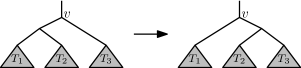
Figure 2: A rooted nearest neighbor interchange prunes a subtree $T_{2}$ from one child of $v$, suppresses the resulting vertex of degree 2 and then grafts $T_{2}$ onto the edge incident to the other child of $v$.

Lemma 3

Let $D$ be a generic ultrametric on $X$ and $T\in{\bf BR}_{X}$ the unique binary rooted phylogenetic tree on $X$ that represents $D$. Then, for any $T^{\prime}\in({\bf BR}_{X}-\{T\})$, there exists an rNNI that changes $T^{\prime}$ to $T^{\prime\prime}\in{\bf BR}_{X}$ with $\sigma_{D}(T^{\prime})>\sigma_{D}(T^{\prime\prime})$.

Proof. We use induction on $n=|X|$. The statement in the lemma clearly holds for $n\in\{1,2\}$ in view of the fact that $|{\bf BR}_{X}|=1$. So assume $n\geq 3$ and consider any $T^{\prime}\in({\bf BR}_{X}-\{T\})$. The situation is depicted in Figure 3(a). Let $A$ and $B$, respectively, denote the set of leaves in the rooted subtrees $T_{1}$ and $T_{2}$ of $T$. Similarly, let $A^{\prime}$ and $B^{\prime}$, respectively, denote the set of leaves in the rooted subtrees $T_{1}^{\prime}$ and $T_{2}^{\prime}$ of $T^{\prime}$. Note that the restriction $D_{|Y}$ of $D$ to any non-empty subset $Y\subseteq X$ is again a generic ultrametric.

First consider the case that $T_{1}^{\prime}$ does not represent $D_{|A^{\prime}}$. Then, by induction, there exists an rNNI in $T_{1}^{\prime}$ that results in a rooted phylogenetic tree $T_{1}^{\prime\prime}$ on $A^{\prime}$ with strictly smaller NEME score. Hence, applying the same rNNI to $T^{\prime}$ yields a tree $T^{\prime\prime}$ with $\sigma_{D}(T^{\prime})>\sigma_{D}(T^{\prime\prime})$. The case that $T_{2}^{\prime}$ does not represent $D_{|B^{\prime}}$ is completely analogous.

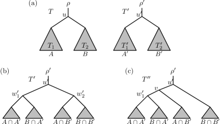
Figure 3: (a) The two trees $T$ and $T^{\prime}$ considered in the proof of Lemma 3. (b) The detailed structure of $T^{\prime}$ in one of the cases considered in the proof. (c) The tree $T^{\prime\prime}$ resulting from a suitable rNNI applied to $T^{\prime}$.

It remains to consider the case that $T_{1}^{\prime}$ and $T_{2}^{\prime}$ represent $D_{|A^{\prime}}$ and $D_{|B^{\prime}}$, respectively. Then, $A=A^{\prime}$ and $B=B^{\prime}$ immediately implies $T_{1}=T_{1}^{\prime}$ and $T_{2}=T_{2}^{\prime}$ and, thus, $T=T^{\prime}$. Otherwise, there exists at least one $\{x,y\}\in\binom{X}{2}$ with $\{x,y\}\subseteq A$ or $\{x,y\}\subseteq B$ but $x\in A^{\prime}$ and $y\in B^{\prime}$. Thus, swapping the roles of either $A$ and $B$ or $A^{\prime}$ and $B^{\prime}$, we can assume without loss of generality that the sets $A\cap A^{\prime}$, $A\cap B^{\prime}$ and $B\cap B^{\prime}$ are non-empty. The structure of the tree $T^{\prime}$ is depicted in Figure 3(b). Put $\omega^{\prime}=\omega_{(D,T^{\prime})}$.

First assume that $B\cap A^{\prime}\neq\emptyset$. Put $n_{1}=|A\cap A^{\prime}|$, $n_{2}=|B\cap A^{\prime}|$, $n_{3}=|A\cap B^{\prime}|$ and $n_{4}=|B\cap B^{\prime}|$. Without loss of generality we assume $n_{1}+n_{2}>n_{4}$. We perform an rNNI pruning and regrafting the subtree with leaf set $A\cap B^{\prime}$ to obtain the tree $T^{\prime\prime}$ depicted in Figure 3(c). Put $\omega^{\prime\prime}=\omega_{(D,T^{\prime\prime})}$. To show $\sigma_{D}(T^{\prime})>\sigma_{D}(T^{\prime\prime})$ it suffices to show $h_{(T^{\prime},\omega^{\prime})}(u^{\prime})+h_{(T^{\prime},\omega^{\prime})}(w_{2}^{\prime})>h_{(T^{\prime\prime},\omega^{\prime\prime})}(u^{\prime})+h_{(T^{\prime\prime},\omega^{\prime\prime})}(v)$. To establish the latter inequality, recall that $T$ represents $D$ and, therefore, we can assume that $D$ has been scaled so that $D(a,b)=1$ for all $a\in A$, $b\in B$. We put

$$\delta_{A}=\sum_{\begin{subarray}{c}a^{\prime}\in(A\cap A^{\prime})\\ b^{\prime}\in(A\cap B^{\prime})\end{subarray}}D(a^{\prime},b^{\prime})\quad\text{and}\quad\delta_{B}=\sum_{\begin{subarray}{c}a^{\prime}\in(B\cap A^{\prime})\\ b^{\prime}\in(B\cap B^{\prime})\end{subarray}}D(a^{\prime},b^{\prime}).$$

Note that all distances that contribute to $\delta_{A}$ and $\delta_{B}$ are strictly less than $1$, implying $\delta_{A}<n_{1}n_{3}$ and $\delta_{B}<n_{2}n_{4}$. Using this notation, we obtain

$$h_{(T^{\prime},\omega^{\prime})}(u^{\prime})+h_{(T^{\prime},\omega^{\prime})}(w_{2}^{\prime})-h_{(T^{\prime\prime},\omega^{\prime\prime})}(u^{\prime})-h_{(T^{\prime\prime},\omega^{\prime\prime})}(v)$$

$$=\frac{1}{2}+\frac{n_{1}n_{4}+n_{2}n_{3}}{2(n_{1}+n_{2})(n_{3}+n_{4})}-\frac{n_{2}}{2(n_{1}+n_{2})}-\frac{n_{1}+n_{3}}{2(n_{1}+n_{2}+n_{3})}$$

$$\quad+\frac{1}{2}\left[\frac{1}{(n_{1}+n_{2})(n_{3}+n_{4})}-\frac{1}{(n_{1}+n_{2})n_{3}}\right]\cdot\delta_{A}$$

$$\quad+\frac{1}{2}\left[\frac{1}{(n_{1}+n_{2})(n_{3}+n_{4})}-\frac{1}{(n_{1}+n_{2}+n_{3})n_{4}}\right]\cdot\delta_{B}$$

$$=g(\delta_{A},\delta_{B}).$$

Note that $g(\delta_{A},\delta_{B})$ is a linear function in $\delta_{A}$ and $\delta_{B}$ and that the coefficient of $\delta_{A}$ is negative. Moreover, the assumption $n_{1}+n_{2}>n_{4}$ implies that the coefficient of $\delta_{B}$ is negative too. Thus, using the fact that $\delta_{A}<n_{1}n_{3}$ and $\delta_{B}<n_{2}n_{4}$, we have

$$g(\delta_{A},\delta_{B})>g(n_{1}n_{3},n_{2}n_{4})=0,$$

from which $\sigma_{D}(T^{\prime})>\sigma_{D}(T^{\prime\prime})$ follows, as required.

It remains to consider the case that $B\cap A^{\prime}=\emptyset$, that is, $n_{2}=0$. We apply the same rNNI to $T^{\prime}$ as in the previous case and, using similar calculations, we obtain

$$\sigma_{D}(T^{\prime})-\sigma_{D}(T^{\prime\prime})=\frac{n_{4}}{2(n_{3}+n_{4})}+\frac{1}{2}\left[\frac{1}{n_{1}(n_{3}+n_{4})}-\frac{1}{n_{1}n_{3}}\right]\cdot\delta_{A}>0,$$

using again $\delta_{A}<n_{1}n_{3}$.  

In the following main result of this section we note that even for the non-generic case a weak form of consistency holds.

Theorem 4

Let $T=(V,E,\rho)\in{\bf BR}_{X}$ and $\omega$ an interior-positive normalized equidistant edge weighting for $T$. Put $D=D_{(T,\omega)}$. Then we have

$$\sigma_{D}(T)=\min\{\sigma_{D}(T^{\prime}):T^{\prime}\in{\bf BR}_{X}\}.$$

If $D$ is generic, then $T$ is the unique tree in ${\bf BR}_{X}$ minimizing the NEME score for $D$ and a local search using rooted nearest neighbor interchanges starting from any tree in ${\bf BR}_{X}$ will arrive at $T$ after a finite number of steps.

Proof. For generic $D$, the theorem is an immediate consequence of Lemma 3. So, assume that $D$ is not generic and, for a contradiction, that there exists some $T^{\prime}\in{\bf BR}_{X}$ with $\sigma_{D}(T^{\prime})<\sigma_{D}(T)$. For any real number $\varepsilon>0$, define the NEEW $\omega_{\varepsilon}$ of $T$ by putting $\omega_{\varepsilon}(e)=\omega(e)+\varepsilon$ for all edges $e$ of $T$ not adjacent to a vertex in $X\cup\{\rho\}$ and $\omega_{\varepsilon}(e)=\omega(e)$ for all other edges $e$ of $T$. Put $D_{\varepsilon}=D_{(T,\omega_{\varepsilon})}$ and note that, by construction, $D_{\varepsilon}$ is a generic ultrametric that is represented by $T$. As a consequence, $\sigma_{D_{\varepsilon}}(T)<\sigma_{D_{\varepsilon}}(T^{\prime})$ must hold. But this contradicts $\sigma_{D}(T^{\prime})<\sigma_{D}(T)$ in view of the fact that, as $\varepsilon$ tends to $0$, $\sigma_{D_{\varepsilon}}(T)$ tends to $\sigma_{D}(T)$ while $\sigma_{D_{\varepsilon}}(T^{\prime})$ tends to $\sigma_{D}(T^{\prime})$.  

The result in Theorem 4 immediately raises the question whether the NEME score for any input distance matrix is minimized by some binary rooted phylogenetic tree. It is known [28] that for unrooted phylogenetic trees the balanced minimum evolution score is indeed always minimized for some unrooted binary phylogenetic tree. We end this section establishing that, in contrast, the answer to the above question for the NEME score is no.

Lemma 5

There exist dissimilarities $D$ with

$$\min\{\sigma_{D}(T):T\in{\bf R}_{X}\}<\min\{\sigma_{D}(T):T\in{\bf BR}_{X}\}.$$

Proof. Consider a binary rooted phylogenetic tree $T$ whose structure is as depicted in Figure 4(a). It consists of two rooted binary subtrees $T_{1}$ and $T_{2}$, each having $m\geq 3$ leaves. In addition, there is a single leaf adjacent to vertex $u$. Let $\omega$ be an interior positive normalized equidistant edge weighting for $T$ such that $h_{(T,\omega)}(v)=1$ and $h_{(T,\omega)}(u)=s$ for some $s>1$. Put $D=D_{(T,\omega)}$.

Next, consider the non-binary rooted phylogenetic tree $T^{\prime}$ depicted in Figure 4(b). It is constructed from $T$ by contracting the edge between $u$ and $v$ into the vertex $w$. Put $\omega^{\prime}=\omega_{(D,T^{\prime})}$. To show that $\sigma_{D}(T)>\sigma_{D}(T^{\prime})$, it suffices, by Equation (1), to show that

$$h_{(T,\omega)}(u)+h_{(T,\omega)}(v) =s+1>2h_{(T^{\prime},\omega^{\prime})}(w)=\frac{2m^{2}+4ms}{m^{2}+2m},$$

which can easily be checked to be the case, in view of $m\geq 3$, for any $s>1$. Hence, by Theorem 4, we have $\min\{\sigma_{D}(T^{\prime}):T^{\prime}\in{\bf R}_{X}\}<\sigma_{D}(T)=\min\{\sigma_{D}(T^{\prime}):T^{\prime}\in{\bf BR}_{X}\}$.  

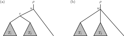
Figure 4: The construction referred to in the proof of Lemma 5.

5 The NEME problem is NP-hard

To establish NP-hardness of the NEME problem, we use a reduction from the well-known NP-hard graph coloring problem (see e.g. [29]). More specifically, we consider the following variant of this problem:
Input: A graph $G=(V,E)$ with $|V|=4n$.
Question: Can $V$ be partitioned into 4 subsets $V_{1},V_{2},V_{3},V_{4}$ with $|V_{1}|=|V_{2}|=|V_{3}|=|V_{4}|=n$ such that no edge $e\in E$ has both endpoints in the same set $V_{i}$ for some $i\in\{1,2,3,4\}$? We call any such partition a 4-coloring of $G$.

Note that the additional constraint that the sets in a 4-coloring are all of the same size is merely added to simplify the description of the reduction. It preserves the NP-hardness of the graph coloring problem in view of the fact that adding isolated vertices to any graph $G$ does not change the minimum number of colors that suffice to color $G$. We first present a technical lemma that will be used in the construction below.

Lemma 6

Let $X$ be a set with $2(m+k)$ elements, $m\geq 1$, $k\geq 1$, that is partitioned into the sets $A$, $B$ and $C$ with $|A|=|B|=m$ and $|C|=2k$. In addition, let $s>0$ be a real number and $D$ a dissimilarity on $X$ with $D(x,y)=s$ for all $x\in A$, $y\in B$ and $D(x,y)\leq\frac{s}{3(m+k)^{5}}$ for all other $x,y\in X$. Then any binary rooted phylogenetic tree $T=(V,E,\rho)$ on $X$ with $\sigma_{D}(T)=\min\{\sigma_{D}(T):T\in{\bf BR}_{X}\}$ must contain two distinct vertices $v,w\in V$ with (i) $C(v)\cap C(w)=\emptyset$, (ii) $|C(v)|=|C(w)|=(m+k)$, (iii) $A\subseteq C(v)$ and $B\subseteq C(w)$.

Proof. First consider a binary rooted phylogenetic tree $T$ on $X$ that contains vertices $v$ and $w$ with properties (i)-(iii). Note that this implies that $v$ and $w$ have the same parent $u$ and that $u$ is the single child of the root $\rho$. Moreover, for all $a\in A$, $b\in B$, we have $\alpha^{T}_{\{a,b\}}=\frac{1}{2(m+k)^{2}}$ and, by Lemma 1(ii), this is the smallest possible value for a rooted phylogenetic tree with $2(m+k)$ leaves.

Next consider any binary rooted phylogenetic tree $T^{\prime}=(V^{\prime},E^{\prime},\rho^{\prime})$ on $X$ that does not contain two vertices $v$ and $w$ satisfying properties (i)-(iii). Let $u^{\prime}$ denote the single child of $\rho^{\prime}$ and consider the two children $v^{\prime}$ and $w^{\prime}$ of $u^{\prime}$. In particular, $v^{\prime}$ and $w^{\prime}$ must violate at least one of the properties (i)-(iii). By construction we have $C(v^{\prime})\cap C(w^{\prime})=\emptyset$. Hence, one of the properties (ii) or (iii) must be violated.

First consider the case that (iii) is violated. This implies, without loss of generality, that there exist $a\in A$ and $b\in B$ with $\{a,b\}\subseteq C(v^{\prime})$. In view of $|C(v^{\prime})|\leq 2(m+k)-1$ and Lemma 1(ii) we have

$$\alpha^{T^{\prime}}_{\{a,b\}}\geq\frac{2}{(2(m+k)-1)^{2}}=\frac{1}{2(m+k)^{2}-2(m+k)+1/2}$$

Next consider the case that property (iii) is satisfied but (ii) is violated for $v^{\prime}$ and $w^{\prime}$. Then, for any $a\in A$ and any $b\in B$, we have

$$\alpha^{T^{\prime}}_{\{a,b\}}\geq\frac{1}{2(m+k+1)(m+k-1)}=\frac{1}{2(m+k)^{2}-2}$$

Noting that $2(m+k)^{2}-2\geq 2(m+k)^{2}-2(m+k)+1/2$, we calculate a lower bound on the difference between the coefficients in $T$ and $T^{\prime}$:

$$\frac{1}{2(m+k)^{2}-2}-\frac{1}{2(m+k)^{2}}\geq\frac{1}{2(m+k)^{4}}.$$

This implies, using Lemma 1(i) to obtain the upper bound in the second line below:

$$\sigma_{D}(T) =\sum_{\{x,y\}\in\binom{X}{2}}\alpha^{T}_{\{x,y\}}D(x,y)$$

$$\leq\left[\sum_{a\in A,\,b\in B}\alpha^{T}_{\{a,b\}}D(a,b)\right]+\frac{s(m+k)}{3(m+k)^{5}}$$

$$<\left[\sum_{a\in A,\,b\in B}\alpha^{T}_{\{a,b\}}s\right]+\frac{s}{2(m+k)^{4}}$$

$$\leq\sum_{a\in A,\,b\in B}\alpha^{T^{\prime}}_{\{a,b\}}s\leq\sum_{\{x,y\}\in\binom{X}{2}}\alpha^{T^{\prime}}_{\{x,y\}}D(x,y)=\sigma_{D}(T^{\prime})$$

Hence, $T^{\prime}$ cannot be an optimal tree for $D$.  

Next we describe how to construct for a given graph $G=(V(G),E(G))$ with $|V(G)|=4n$ a suitable dissimilarity $D=D(G)$. First construct a set $X$ that is the disjoint union of $V(G)$, $Y$ and $W$ with $|Y|=2^{k}$ and $|W|=(2^{k}-4)n$ where $k=\lfloor\log_{2}(n+1)+4\rfloor$. Note that

$$|X|=2^{k}(n+1)\leq 2^{\log_{2}(n+1)+4}(n+1)=16(n+1)^{2}.$$

Put $m_{i}=2^{k-i}(n+1)$, $i\in\{0,1,\dots,k\}$. In addition, put $s_{1}=1$ and, for $i\in\{1,2,\dots,k\}$, $s_{i+1}=\frac{s_{i}}{3m_{i}^{5}}$. Moreover, put $s^{*}=\frac{s_{k+1}}{2^{k+2}(n+1)^{3}}$. The values $s_{1}>s_{2}>\dots>s_{k+1}>s^{*}>0$ will be the possible distances between elements in $X$.

Now, recursively partition the set $Y$ so as to force a fully balanced binary tree as a backbone structure. More precisely, put $Y_{0,0}=Y$ and define, for all $i\in\{0,1,\dots,k-1\}$ and all $j\in\{0,1,\dots,2^{i}-1\}$, sets $Y_{i+1,2j}$ and $Y_{i+1,2j+1}$ so that $Y_{i+1,2j}\cap Y_{i+1,2j+1}=\emptyset$, $Y_{i+1,2j}\cup Y_{i+1,2j+1}=Y_{i,j}$ and $|Y_{i+1,2j}|=|Y_{i+1,2j+1}|$ hold. Select an element $y_{l}^{*}\in Y_{2,l}$ for each $l\in\{0,1,2,3\}$.

Next we construct the dissimilarity $D=D(G)$ on $X$:

• For all $w\in W$ and all $x\in X$ we put $D(w,x)=0$. The elements in $W$ are just used to fill subtrees so that we get a fully balanced backbone tree.

• For all $y,y^{\prime}\in Y$, $y\neq y^{\prime}$, we put $D(y,y^{\prime})=s_{i+1}$ where $i$ is the largest index in $\{0,1,\dots,k-1\}$ with $\{y,y^{\prime}\}\subseteq Y_{i,j}$ for some $j\in\{0,1,\dots,2^{i}-1\}$. The distances between the elements in $Y$ force a fully balanced backbone tree by Lemma 6 (cf. Figure 5).

• For all $v\in V(G)$ and all $y\in(Y-\{y_{1}^{*},y_{2}^{*},y_{3}^{*},y_{4}^{*}\})$ we put $D(v,y)=s_{k+1}$. And for all $v\in V(G)$ and all $y\in\{y_{1}^{*},y_{2}^{*},y_{3}^{*},y_{4}^{*}\}$ we put $D(v,y)=0$. This will force that a subset of $n$ vertices of $G$ is grouped together with each $y_{l}^{*}$, $1\leq l\leq 4$, in the same subtree.

• For all $v,v^{\prime}\in V(G)$, $v\neq v^{\prime}$, we put $D(v,v^{\prime})=s^{*}$ if $\{v,v^{\prime}\}\in E(G)$ and $D(v,v^{\prime})=0$ otherwise. These distances capture the structure of $G$ and are so small that they do not interfere with forming the fully balanced backbone tree.

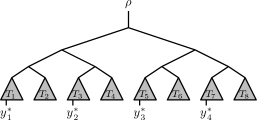
Figure 5: The structure of the backbone tree for $k=3$.

Lemma 7

Let $G$ be a graph with $4n$ vertices and let $D=D(G)$ be the dissimilarity on $X$ constructed above. Then $G$ has a 4-coloring if and only if there exists a binary rooted phylogenetic tree $T$ on $X$ with $\sigma_{D}(T)$ not larger than

$$\left[2^{k-2}\sum_{i=1}^{k}\frac{s_{i}}{m_{i}^{2}}\right]+s_{k+1}\cdot 4n\cdot\left[\left(\sum_{i=0}^{k-3}\frac{2^{i}}{2m_{k-i}^{2}}\right)+\frac{2^{k-2}-1}{2m_{2}^{2}}+\frac{2^{k-1}-2}{2m_{1}^{2}}\right]+\frac{s^{*}}{2^{2k-7}}$$

Proof. First note that, by the construction of the distances $s_{1},s_{2},\dots,s_{k+1},s^{*}$ and Lemma 6, the upper part of any optimal binary rooted phylogenetic tree $T$ on $X$ must be a fully balanced binary tree. This upper part has $k+1$ levels. Level $i\in\{0,1,\dots,k\}$ consists of $2^{i}$ subtrees, each of which containing precisely one of the sets $Y_{i,j}$, $j\in\{0,1,\dots,2^{i}-1\}$ in its set of leaves. In particular, the lowest level consists of $2^{k}$ subtrees $T_{1},T_{2},\dots,T_{2^{k}}$ and the leaf set of each of these subtrees consists of precisely one element from $Y$ and $n$ elements from $V(G)\cup W$. Thus, in view of $y^{*}_{l}\in Y_{2,l}$, $l\in\{0,1,2,3\}$, we can choose the numbering of the subtrees so that $T_{l2^{k-2}+1}$ is the subtree that contains leaf $y^{*}_{l}$ (cf. Figure 5).

Now consider any vertex $v\in V(G)$. First assume that $v$ is a leaf in one of the subtrees $T_{l2^{k-2}+1}$, $l\in\{0,1,2,3\}$. Then, because the backbone tree is fully balanced, the contribution to $\sigma_{D}(T)$ of the distances from $v$ to the elements in $Y$ is

$$s_{k+1}\cdot\left[\left(\sum_{i=0}^{k-3}\frac{2^{i}}{2m_{k-i}^{2}}\right)+\frac{2^{k-2}-1}{2m_{2}^{2}}+\frac{2^{k-1}-2}{2m_{1}^{2}}\right].$$

Next assume that $v$ is a leaf in some subtree $T_{q}$, $q\neq l2^{k-2}+1$ for all $l\in\{0,1,2,3\}$. Then one summand of the form $\frac{s_{k+1}}{2m_{k-i}^{2}}$, $i\in\{0,1,\dots,k-3\}$, is replaced by a summand that contributes, by Equation (3), at least $\frac{1}{2(m_{k}/2)^{2}}\cdot s_{k+1}=\frac{2s_{k+1}}{m_{k}^{2}}=\frac{2s_{k+1}}{(n+1)^{2}}$. Thus, the increase in the contribution is at least

$$\left[\frac{2}{m_{k}^{2}}-\frac{1}{2m_{k}^{2}}\right]\cdot s_{k+1}=\frac{3s_{k+1}}{2(n+1)^{2}}>2^{k-1}(n+1)s^{*}\geq\sum_{\{x,y\}\in\binom{X}{2}}\alpha^{T}_{\{x,y\}}s^{*},$$

that is, using Lemma 1(i) to obtain the last inequality, it is strictly larger than the total contribution of all distances that equal $s^{*}$. Hence, the contribution of the distances $s_{k+1}$ to the score is minimized if and only if each vertex $v\in V(G)$ is a leaf in one of the subtrees $T_{l}$, $1\leq l\leq 4$, inducing a partition of $V(G)$ into 4 subsets $V_{1},V_{2},V_{3},V_{4}$ each of size $n$.

Summarizing the contribution of the distances $s_{1},s_{2},\dots,s_{k+1}$ to the score of the tree, we obtain:

$$\lambda(n,k)=\left[2^{k-2}\sum_{i=1}^{k}\frac{s_{i}}{m_{i}^{2}}\right]+s_{k+1}\cdot 4n\cdot\left[\left(\sum_{i=0}^{k-3}\frac{2^{i}}{2m_{k-i}^{2}}\right)+\frac{2^{k-2}-1}{2m_{2}^{2}}+\frac{2^{k-1}-2}{2m_{1}^{2}}\right]$$

Note that this contribution does not depend on the structure of the graph $G$.

It remains to calculate the contribution of the distances that equal $s^{*}$ to the score of the tree. Note that $16(n+1)^{2}$ is a trivial upper bound on the number of edges in $G$. Thus, if the partition $V_{1},V_{2},V_{3},V_{4}$ induced by the tree is a 4-coloring of $G$, then the total contribution to the score of the tree is at most

$$\frac{16(n+1)^{2}s^{*}}{2m_{2}^{2}}=\frac{16s^{*}}{2^{2k-3}}=\frac{s^{*}}{2^{2k-7}}.$$

In contrast, a single edge with both endpoints in one of the sets $V_{l}$, $1\leq l\leq 4$, contributes, by Equation (3), at least $\frac{1}{2((n+1)/2)^{2}}s^{*}=\frac{2s^{*}}{(n+1)^{2}}$. Hence, noting that $k=\lfloor\log_{2}(n+1)+4\rfloor$ implies $\frac{2}{(n+1)^{2}}>\frac{1}{2^{2k-7}}$, we obtain that $G$ has a 4-coloring if and only if there exists a binary rooted phylogenetic tree $T$ on $X$ with

$$\sigma_{D}(T)\leq\lambda(n,k)+\frac{s^{*}}{2^{2k-7}}.$$

 

Note that the dissimilarity $D=D(G)$ constructed above need not satisfy the triangle inequality. However, putting $D^{\prime}(x,x^{\prime})=D(x,x^{\prime})+1$ for all $x,x^{\prime}\in X$, $x\neq x^{\prime}$, and $D^{\prime}(x,x)=0$ for all $x\in X$, we obtain a dissimilarity $D^{\prime}$ on $X$ that satisfies the triangle inequality. Moreover, by Lemma 1(i), for every binary rooted phylogenetic tree $T$ on $X$, we have $\sigma_{D^{\prime}}(T)=\sigma_{D}(T)+\frac{1}{2}(|X|-1)$, that is, a tree $T$ is optimal for $D$ if and only if $T$ is optimal for $D^{\prime}$. Thus we have the main result of this section:

Theorem 8

Computing a binary rooted phylogenetic tree with minimum NEME score for a dissimilarity $D^{\prime}$ on a set $X$ is NP-hard even if $D^{\prime}$ satisfies the triangle inequality and $D^{\prime}$ takes on only $O(\log_{2}(|X|))$ different values.

6 Approximating the minimum NEME score

Note that Lemma 1(iii) states that any tree in ${\bf R}_{X}$ approximates the minimum NEME score over all trees in ${\bf R}_{X}$ up to a factor that is in $O(n^{2})$, $n=|X|$. It is not hard to see that this bound is asymptotically tight and in this section we explore ways to obtain better approximation guaranties.

We first look at the approximation gaurantees that can be achieved with existing algorithms. We start with UPGMA and establish a lower bound of $\Omega(n)$ on the approximation guaranty achieved by it.

Lemma 9

For every non-empty finite set $X$ with $n\geq 3$ elements there exists a dissimilarity $D$ on $X$ such that

$$\sigma_{D}(T)\geq\frac{n}{4}\min\{\sigma_{D}(T^{\prime}):T^{\prime}\in{\bf R}_{X}\}$$

holds for the tree $T$ produced by UPGMA.

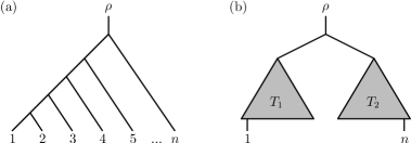
Figure 6: Two rooted phylogenetic trees used in the proof of Lemma 9.

Proof. Let $X=\{1,2,\dots,n\}$ and consider the ultrametric $D^{\prime}$ on $X$ defined by putting, for all $1\leq i<j\leq n$, $D^{\prime}(i,j)=D^{\prime}(j,i)=1+\frac{(j-2)}{n-2}$. Note that the unique rooted phylogenetic tree $T$ on $X$ with $D_{(T,\omega)}=D^{\prime}$ for some interior positive normalized equidistant edge weighting $\omega$ is the rooted caterpillar depicted in Figure 6(a). This is also the tree constructed by UPGMA on input $D^{\prime}$.

From $D^{\prime}$ we construct the dissimilarity $D$ by putting $D(x,y)=D^{\prime}(x,y)$, for all $\{x,y\}\in\left(\binom{X}{2}-\{\{1,n\}\}\right)$, and $D(1,n)=D(n,1)=s$ for some constant $s>2$. Note that UPGMA will still generate the tree $T$ on input $D$ and that $\sigma_{D}(T)\geq\frac{s}{2(n-1)}$ holds.

Now consider any binary rooted phylogenetic tree $T^{\prime}$ on $X$ whose structure is as depicted in Figure 6(b). More specifically, the rooted subtree $T_{1}$ has $\lfloor\frac{n}{2}\rfloor$ leaves, one of them being $1$, and $T_{2}$ has $\lceil\frac{n}{2}\rceil$ leaves, one of them being $n$. Using Lemma 1(i) and the fact that $D^{\prime}(x,y)\leq 2$ for all $\{x,y\}\in\binom{X}{2}$, we have

$$\sigma_{D}(T^{\prime})\leq\alpha^{T^{\prime}}_{\{1,n\}}\cdot D(1,n)+\sum_{\{x,y\}\in\binom{X}{2}}\alpha^{T^{\prime}}_{\{x,y\}}\cdot D^{\prime}(x,y)\leq\frac{2s}{n^{2}-1}+(n-1),$$

implying that $\frac{n}{4}\sigma_{D}(T^{\prime})\leq\frac{s}{2(n-1)}\leq\sigma_{D}(T)$ for $s\geq\frac{1}{2}n(n+1)(n-1)^{2}$. But this implies $\sigma_{D}(T)\geq\frac{n}{4}\min\{\sigma_{D}(T^{\prime}):T^{\prime}\in{\bf R}_{X}\}$, as required.  

Next we briefly touch upon another potential approach from the literature for approximating the minimum NEME score. To describe this approach, note that the NEME problem is related to the problem of finding a sparsest cut, that is, given a dissimilarity $D$ on a finite set $X$ compute a split $A|B$ of $X$, that is, a bipartition of $X$ into two non-empty subsets $A$ and $B$, such that

$$\frac{1}{|A|\cdot|B|}\sum_{a\in A,\,b\in B}D(a,b)$$

is minimum. This problem is usually stated in terms of edge weighted graphs and known to be NP-hard. Recent work on this problem mainly concentrated in finding good approximations of a sparsest cut (see e.g. [30]).

Interestingly, a greedy top-down analogy of UPGMA based on recursively splitting $X$ by sparsest cuts has been proposed for detecting hierarchical community structure of social networks [31]. Using again the dissimilarity $D$ described in the proof of Lemma 2, it can be seen, however, that this approach can yield trees whose NEME score is worse by a quadratic factor in $|X|$ than the minimum NEME score.

In view of the fact that the approaches we explored so far have not led to good approximation guaranties, we apply in the following a generic approach from the literature to establish a polylogarithmic approximation guaranty for dissimilarities that satisfy the triangle inequality, that is, metrics. This approach relies on two ingredients:

• The existence of a polynomial time algorithm with polylogarithmic approximation guaranty for treelike metrics.

• The fact [32] that there exists a polynomial time algorithm that computes, for any metric $D$ on a set $X$ with $n$ elements, a collection $D_{1},D_{2},\dots,D_{k}$ of treelike metrics on $X$ along with positive coefficients $\beta_{1},\beta_{2},\dots,\beta_{k}$, $\beta_{1}+\beta_{2}+\dots+\beta_{k}=1$, such that

  • $D(x,y)\leq D_{i}(x,y)$ for all $i\in\{1,2,\dots,k\}$ and all $x,y\in X$, and

  • there exists a constant $c>0$ such that

    $$\sum_{i=1}^{k}\beta_{i}D_{i}(x,y)\leq c\cdot\log_{2}(n)\cdot D(x,y)$$

    for all $x,y\in X$.

We shall first establish (i). To this end, we rely on the following fact that, phrased in various guises, seems to be mathematical folklore. For the convenience of the reader we provide a short proof and phrase it in terms of splits in unrooted binary phylogenetic trees, that is, trees obtained from rooted binary phylogenetic trees by removing the root and the edge incident with it, and then suppressing the resulting degree two vertex. Recall that each edge $e$ in an unrooted binary phylogenetic tree $T$ on $X$ induces a split $S_{e}=A_{e}|B_{e}$ of $X$ in which $A_{e}$ and $B_{e}$ are the leaf sets of the two connected components resulting from removing $e$ from $T$.

Lemma 10

In every unrooted binary phylogenetic tree $T$ on $X$ with $|X|\geq 2$ there exists an edge $e$ such that the split $A_{e}|B_{e}$ of $X$ satisfies

$$\frac{1}{3}n\leq\min\{|A_{e}|,|B_{e}|\}\leq\max\{|A_{e}|,|B_{e}|\}\leq\frac{2}{3}n.$$ (6)

Proof. Assume that such an edge does not exist. Replace all edges $e$ of $T$ by a directed edge in such a way that this directed edge points to the larger of the two sets $A_{e}$ and $B_{e}$. Then every directed edge incident with a leaf of $T$ is directed away from that leaf and, in view of the fact that all other vertices of $T$ have degree three, one of those vertices must be such that all three directed edges incident with this vertex $v$ are directed towards it. But this implies that, while all edges $e$ incident with $v$ must clearly satisfy $\min\{|A_{e}|,|B_{e}|\}\leq\frac{n}{2}$, by the pigeonhole principle, at least one of these edges must also satisfy $\min\{|A_{e}|,|B_{e}|\}\geq\frac{n}{3}$, contradicting our assumption.  

Note that Lemma 10 does not hold for non-binary trees. The next lemma establishes (i). Recall that a treelike metric on $X$ is a metric for which there exists an unrooted phylogenetic tree $T^{\prime}$ on $X$ with a non-negative edge-weighting $\omega^{\prime}$ with $D=D_{(T^{\prime},\omega^{\prime})}$.

Lemma 11

Let $D$ be a treelike metric on a set $X$ with $n$ elements. Then a binary rooted phylogenetic tree $T$ on $X$ with

$$\sigma_{D}(T)\leq c\cdot\log_{2}(n)\cdot\min\{\sigma_{D}(T^{\prime}):T^{\prime}\in{\bf BR}_{X}\}$$

for some positive constant $c$ can be computed in time $O(n^{2})$.

Proof. Let $T^{\prime}=(V^{\prime},E^{\prime})$ be a binary unrooted phylogenetic tree on $X$ and $\omega^{\prime}$ a non-negative edge weighting of $T^{\prime}$ with $D=D_{(T^{\prime},\omega^{\prime})}$. For every edge $e\in E^{\prime}$ we denote by $D_{e}$ the metric that assigns 1 to a pair $(x,y)\in X\times X$ if the path from $x$ to $y$ in $T$ contains edge $e$. Otherwise $D_{e}$ assigns the value 0 to $(x,y)$. Then $D=\sum_{e\in E^{\prime}}\omega^{\prime}(e)\cdot D_{e}(x,y)$ and hence by Equation (5) we have, for any rooted phylogenetic tree $T$ on $X$,

$$\sigma_{D}(T) =\sum_{e\in E^{\prime}}\omega^{\prime}(e)\sigma_{D_{e}}(T)\geq\sum_{e\in E^{\prime}}\frac{\omega^{\prime}(e)}{2},$$

where the last inequality follows from the fact that, for all $e\in E^{\prime}$, $D_{e}$ is an ultrametric and, therefore, $\min\{\sigma_{D_{e}}(T^{\prime\prime}):T^{\prime\prime}\in{\bf BR}_{X}\}=\frac{1}{2}$ by Theorem 4.

Hence, it suffices to show how to construct in polynomial time a rooted phylogenetic tree $T$ on $X$ with $\sigma_{D}(T)\leq c\cdot\log_{2}(n)\cdot\sum_{e\in E^{\prime}}\frac{\omega^{\prime}(e)}{2}$ for some constant $c>0$. This is done recursively as follows. Using Lemma 10, we find an edge $e\in E^{\prime}$ such that the split $S_{e}=A_{e}|B_{e}$ of $X$ induced by $e$ satisfies (6). We require that the resulting rooted phylogenetic tree $T$ on $X$ will have the clusters $A_{e}$ and $B_{e}$. Then we remove $e$ from $T^{\prime}$. This yields, after suppressing the two vertices of degree 2, two unrooted phylogenetic trees $T^{\prime}_{A_{e}}$ on $A_{e}$ and $T^{\prime}_{B_{e}}$ on $B_{e}$ which represent the restriction of $D$ to $A_{e}$ and $B_{e}$, respectively. If $|A_{e}|>1$ ($|B_{e}|>1$) we construct a binary rooted phylogenetic tree $T_{A_{e}}$ on $A_{e}$ ($T_{B_{e}}$ on $B_{e}$) recursively. Otherwise $T_{A_{e}}$ ($T_{B_{e}}$) is the unique rooted phylogenetic tree on $A_{e}$ ($B_{e}$). Then we glue the roots of $T_{A_{e}}$ and $T_{B_{e}}$ together and add a new root $\rho$ to obtain a binary rooted phylogenetic tree $T=(V,E,\rho)$ on $X$. Note that this construction can clearly be done in time $O(n^{2})$ and, since we choose the edges for recursively partitioning $T^{\prime}$ in such a way that Inequalities (6) hold, it follows that every path in $T$ contains $O(\log_{2}(n))$ vertices.

Figure 7: An illustration of the canonical map $\varphi$ used in the proof of Lemma 11: (i) An unrooted binary phylogenetic tree $T^{\prime}$ on $X=\{1,2,\cdots,7\}$ (for simplicity, the label $e_{i}$ of the edge incident with leaf $i$ is omitted). (ii) A binary rooted phylogenetic tree on $X$ constructed from $T^{\prime}$ by consecutively removing the following sets of edges $\{e_{10}\},\{e_{8}\},\{e_{5},e_{11}\},\{e_{3},e_{4},e_{9}\},\{e_{6},e_{7}\},\{e_{1},e_{2}\}$. Then the canonical map $\varphi$ is as follows: $\varphi(e_{10})=u_{1},\varphi(e_{8})=u_{2},\varphi(e_{5})=\varphi(e_{11})=u_{5},\varphi(e_{3})=\varphi(e_{4})=\varphi(e_{9})=u_{4},\varphi(e_{6})=\varphi(e_{7})=u_{6},$ and $\varphi(e_{1})=\varphi(e_{2})=u_{3}$.

Note that the construction of $T$ induces the canonical map $\varphi:E^{\prime}\rightarrow(V-(X\cup\{\rho\}))$ that assigns to $e\in E^{\prime}$ the internal vertex $v$ of $T$ that was constructed as the root in a recursive step when edge $e$ was removed from $T^{\prime}$ (see Fig. 7 for an example). Also note that $\varphi$ is, by construction, surjective. It is, however, not injective because suppressing degree 2 vertices leads to clusters of original edges in $T^{\prime}$ that are removed together at a single recursive step.

Next, for each edge $e\in E^{\prime}$ let $\omega_{e}=\omega_{(D_{e},T)}$ and let $\Gamma_{e}$ be the set of those vertices $v\in(V-(X\cup\{\rho\}))$ for which there exist $x,y\in X$ such that (i) $v=lca(x,y)$ and (ii) $e$ lies on the path from $x$ to $y$ in $T^{\prime}$. By construction of $T$, the set $\Gamma_{e}$ consists precisely of those vertices in $V-(X\cup\{\rho\})$ that lie on the path from $\varphi(e)$ to $\rho$ in $T$, implying that $|\Gamma_{e}|\in O(\log_{2}(n))$. In addition, Equation (2) implies that $D_{e}$ contributes at most $1/2$ to $h_{(T,\omega_{e})}(v)$ for all $v\in\Gamma_{e}$ and, for all $v\in V-\Gamma_{e}$ we have $h_{(T,\omega_{e})}(v)=0$. Therefore, using Equation (1) to obtain the second equality below, we have

$$\sigma_{D}(T) = \sum_{e\in E^{\prime}}\omega^{\prime}(e)\sigma_{D_{e}}(T)$$ (7)

$$= \sum_{e\in E^{\prime}}\omega^{\prime}(e)\Big{(}\sum_{v\in(V-(X\cup\{\rho\}))}h_{(T,\omega_{e})}(v)\Big{)}$$

$$= \sum_{e\in E^{\prime}}\omega^{\prime}(e)\Big{(}\sum_{v\in\Gamma_{e}}h_{(T,\omega_{e})}(v)\Big{)}$$

$$\leq c\cdot\log_{2}(n)\cdot\sum_{e\in E^{\prime}}\frac{\omega^{\prime}(e)}{2}$$

for some constant $c>0$, as required.  

Note that there are treelike metrics $D$ on $X$ for which a binary rooted phylogenetic tree with minimum NEME score cannot be obtained by rooting the unrooted tree representing $D$ somewhere. That means that the structure of the unrooted tree representing $D$ need not reflect much the structure of the rooted trees with minimum NEME score for $D$. Consider, for example, the metric $D$ on $X=\{1,2,\dots,n\}$, $n\geq 6$, induced by the unrooted caterpillar in Figure 8. All edges are assigned weight 1. Then the recursive algorithm in the proof of Lemma 11 yields a binary rooted phylogenetic tree $T$ on $X$ with $\sigma_{D}(T)\in O(n\log_{2}n)$ by the upper bound in (7). In contrast, for any binary rooted phylogenetic tree $T^{\prime}$ obtained by rooting the caterpillar, there must exist, for all $k\in\{3,4,\dots,\lfloor\frac{n}{2}\rfloor\}$, at least one vertex $v$ in $T^{\prime}$ with $|ch(v)|=k$ and $h_{(T^{\prime},\omega)}(v)\geq\frac{1}{2(k-1)}(k+(k-1)+\dots+4+3)\geq\frac{k}{4}$, where $\omega=\omega_{(D,T^{\prime})}$. This implies that $\sigma_{D}(T^{\prime})\geq\sum_{k=3}^{\lfloor\frac{n}{2}\rfloor}\frac{k}{4}\in\Omega(n^{2})$. The next theorem summarizes our results on approximating the NEME score for metrics.

Figure 8: An unrooted caterpillar tree on $X=\{1,2,\dots,n\}$. The metric $D$ induced by this tree on $X$ (all edges have weight 1) is such that a rooted phylogenetic tree on $X$ with minimum NEME score for $D$ cannot by obtained by rooting the caterpillar somewhere.

Theorem 12

Let $D$ be a metric on a finite set $X$ with $n$ elements. Then a rooted binary phylogenetic tree $T$ on $X$ with

$$\sigma_{D}(T)\leq c\cdot\log^{2}(n)\cdot\min\{\sigma_{D}(T^{\prime}):T^{\prime}\in{\bf BR}_{X}\}$$

for some positive constant $c$ can be computed in polynomial time.

Proof. Let $D_{1},D_{2},\dots,D_{k}$ be a collection of treelike metrics for $D$ together with coefficients $\beta_{1},\beta_{2},\dots,\beta_{k}$ as described in (ii) above. In addition, let $T^{*}$ be a binary rooted phylogenetic tree on $X$ with minimum NEME score for $D$ and, similarly, $T_{i}^{*}$ be a binary rooted phylogenetic tree on $X$ with minimum NEME score for $D_{i}$, $1\leq i\leq k$. Assume that $\sigma_{D_{1}}(T_{1}^{*})\leq\sigma_{D_{i}}(T_{i}^{*})$ for all $i\in\{1,2,\dots,k\}$. Finally, let $T_{1}^{o}$ be the binary rooted phylogenetic tree on $X$ constructed for $D_{1}$ using the recursive algorithm in the proof of Lemma 11. Then we have, using repeatedly the linearity from Equation (5):

$$\sigma_{D}(T_{1}^{o}) \leq\sigma_{D_{1}}(T_{1}^{o})$$

$$\leq c^{\prime}\cdot\log_{2}(n)\cdot\sigma_{D_{1}}(T_{1}^{*})$$

$$\leq c^{\prime}\cdot\log_{2}(n)\cdot\sum_{i=1}^{k}\beta_{i}\cdot\sigma_{D_{i}}(T_{i}^{*})$$

$$\leq c^{\prime}\cdot\log_{2}(n)\cdot\sum_{i=1}^{k}\beta_{i}\cdot\sigma_{D_{i}}(T^{*})$$

$$=c^{\prime}\cdot\log_{2}(n)\cdot\sigma_{(\sum_{i=1}^{k}\beta_{i}\cdot D_{i})}(T^{*})$$

$$\leq c^{\prime}c^{\prime\prime}\cdot\log_{2}^{2}(n)\cdot\sigma_{D}(T^{*}),$$

where $c^{\prime}$ and $c^{\prime\prime}$ are positive constants that come from the upper bound (7) and property (2) of the collection $D_{1},D_{2},\dots,D_{k}$, respectively. Hence $\sigma_{D}(T_{1}^{o})\leq c\cdot\log_{2}^{2}(n)\cdot\sigma_{D}(T^{*})$ for some constant $c>0$ and the tree $T_{1}^{o}$ can be constructed in polynomial time.  

Interestingly, the above approach can be applied to any variant of minimum evolution as long as the objective function is a linear combination of the input distances and the variant is consistent (the latter trivially implies ingredient (i) above and, thus, saves a factor of $\log n$ in the approximation guaranty). In particular, the original unrooted ME problem [11] has these properties and can, therefore, be approximated for metrics within a factor of $O(\log_{2}n)$. To the best of our knowledge, this is the first non-trivial approximation result for the unrooted ME problem.

7 Concluding remarks and open problems

In this paper, we have highlighted some properties of the UPGMA method. We now conclude by pointing out two possible directions for future work. The first direction concerns improving the approximation guarantee for the NEME problem presented in the last section. Recall that the interpretation of the balanced minimum evolution score of an unrooted tree as an average over spanning cycles has been used (as one ingredient amongst others) in [17] to design a constant-factor polynomial time approximation algorithm for the balanced minimum evolution problem in case the given dissimilarity satisfies the triangle inequality. We expect that the results presented in this paper can similarly serve as the basis for a better understanding of the approximation properties of the NEME problem. A concrete conjecture we have in this direction is that UPGMA always generates a tree whose NEME score is within a factor in $O(n)$ of the minimum score.

The second direction for future work concerns the so-called safety radius of the NEME approach for computing rooted phylogenetic trees. The safety radius concept was introduced to quantify how much distortion of the input distance matrix a method can tolerate and still return the correct tree (see e.g. [33]). For example, it is known that in the rooted-tree setting UPGMA has a safety radius of 1 [34], and that both neighbor joining and BME-based tree construction have a safety radius of $\frac{1}{2}$ (see [33] and [35], respectively). We conjecture that the safety radius of NEME-based tree construction tends to 0 as the number of leaves of the trees tends to infinity. In this context, it might also be of interest to study the stochastic safety radius of the NEME problem, a concept that was recently introduced [36], and which aims to understand consistency within a probabilistic setting.

References

References

- [1] P. D’haeseleer, How does gene expression clustering work?, Nature biotechnology 23 (12) (2005) 1499–1501.
- [2] R. Sokal, C. Michener, A statistical method for evaluating systematic relationships, University of Kansas Science Bulletin 38 (1958) 1409–1438.
- [3] Y. Loewenstein, E. Portugaly, M. Fromer, M. Linial, Efficient algorithms for accurate hierarchical clustering of huge datasets: tackling the entire protein space, Bioinformatics 24 (13) (2008) i41–i49.
- [4] J. Felsenstein, Inferring phylogenies, Sinauer associates Sunderland, 2004.
- [5] P. Legendre, L. Legendre, Numerical ecology, Vol. 24, Elsevier, 2012.
- [6] W. Li, L. Fu, B. Niu, S. Wu, J. Wooley, Ultrafast clustering algorithms for metagenomic sequence analysis, Briefings in bioinformatics 13 (6) (2012) 656–668.
- [7] C. Romesburg, Cluster analysis for researchers, Lulu. com, 2004.
- [8] R. Davidson, S. Sullivant, Polyhedral combinatorics of UPGMA cones, Advances in Applied Mathematics 50 (2) (2013) 327–338.
- [9] O. Gascuel, M. Steel, Neighbor-Joining revealed, Molecular Biology and Evolution 23 (2006) 1997–2000.
- [10] N. Saitou, M. Nei, The Neighbor-Joining method: a new method for reconstructing phylogenetictrees, Molecular Biology and Evolution 4 (1987) 406–425.
- [11] A. Rzhetsky, M. Nei, Theoretical foundation of the minimum-evolution method of phylogenetic inference, Molecular Biology and Evolution 10 (1993) 1073–1095.
- [12] R. Agarwala, V. Bafna, M. Farach, M. Paterson, M. Thorup, On the approximability of numerical taxonomy (fitting distances by tree metrics), SIAM Journal on Computing 28 (1998) 1073–1085.
- [13] W. Day, Computational complexity of inferring phylogenies from dissimilarity matrices, Bulletin of Mathematical Biology 49 (1987) 461–467.
- [14] M. Farach, S. Kannan, T. Warnow, A robust model for finding optimal evolutionary trees, Algorithmica 13 (1995) 155–179.
- [15] D. Catanzaro, The minimum evolution problem: overview and classification, Networks 53 (2009) 112–125.
- [16] R. Desper, O. Gascuel, Theoretical foundation of the balanced minimum evolution method of phylogenetic inference and its relationship to weighted least-squares tree fitting, Molecular Biology and Evolution 21 (3) (2004) 587–598.
- [17] S. Fiorini, G. Joret, Approximating the balanced minimum evolution problem, Operation Research Letters 40 (2012) 31–35.
- [18] S. Bastkowski, V. Moulton, A. Spillner, T. Wu, The minimum evolution problem is hard: a link between tree inference and graph clustering problems, Bioinformatics 32 (4) (2016) 518–522.
- [19] C. Semple, M. Steel, Cyclic permutations and evolutionary trees, Advances in Applied Mathematics 32 (2004) 669–680.
- [20] C. Fahey, S. Hosten, N. Krieger, L. Timpe, Least squares methods for equidistant tree reconstruction, available online at arXiv:0808.3979 (2008).
- [21] F. Pardi, O. Gascuel, Combinatorics of distance-based tree inference, Proceedings of the National Academy of Sciences of the USA 109 (2012) 16443–16448.
- [22] M. Bordewich, O. Gascuel, K. Huber, V. Moulton, Consistency of topological moves based on the balanced minimum evolution principle of phylogenetic inference, IEEE/ACM Transactions on Computational Biology and Bioinformatics 6 (2009) 110–117.
- [23] M. Bordewich, R. Mihaescu, Accuracy guarantees for phylogeny reconstruction algorithms based on balanced minimum evolution, IEEE/ACM Transactions on Computational Biology and Bioinformatics 10 (2013) 576–583.
- [24] J. Farris, On the cophenetic correlation coefficient, Systematic Biology 18 (1969) 279–285.
- [25] W. Vach, Least squares approximation of addititve trees, in: Conceptual and Numerical Analysis of Data, Springer, 1989, pp. 230–238.
- [26] S. Willson, Consistent formulas for estimating the total lengths of trees, Discrete Applied Mathematics 148 (2005) 214–239.
- [27] C. Semple, M. Steel, Phylogenetics, Oxford University Press, 2003.
- [28] K. Eickmeyer, P. Huggins, L. Pachter, R. Yoshida, On the optimality of the Neighbor-Joining algorithm, Algorithms for Molecular Biology 3 (2008) 1–11.
- [29] M. Garey, D. Johnson, Computers and intractability: a guide to the theory of NP-completeness, Freeman, 1979.
- [30] S. Arora, E. Hazan, S. Kale, approximation to SPARSEST CUT in time, SIAM Journal on Computing 39 (2010) 1748–1771.
- [31] C. Mann, D. Matula, E. Olinick, The use of sparsest cuts to reveal the hierarchical community structure of social networks, Social Networks 30 (2008) 223–234.
- [32] J. Fakcharoenphol, S. Rao, K. Talwar, A tight bound on approximating arbitrary metrics by tree metrics, Journal of Computer and System Sciences 69 (2004) 485–497.
- [33] K. Atteson, The performance of neighbor-joining methods of phylogenetic reconstruction, Algorithmica 25 (2-3) (1999) 251–278.
- [34] O. Gascuel, A. McKenzie, Performance analysis of hierarchical clustering algorithms, Journal of Classification 21 (2004) 3–18.
- [35] F. Pardi, S. Guillemot, O. Gascuel, Robustness of phylogenetic inference based on minimum evolution, Bulletin of Mathematical Biology 72 (2010) 1820–1839.
- [36] O. Gascuel, M. Steel, A stochastic safety radius for distance-based tree reconstruction, Algorithmica (2015) 1–18.