Itinerant ferromagnetism of two-dimensional repulsive fermions with Rabi coupling

Abstract

We study a two-dimensional fermionic cloud of repulsive alkali-metal atoms characterized by two hyperfine states which are Rabi coupled. Within a variational Hartree-Fock scheme, we calculate analytically the ground-state energy of the system. Then we determine the conditions under which there is a quantum phase transition with spontaneous symmetry breaking from a spin-balanced configuration to a spin-polarized one, an effect known as itinerant ferromagnetism. Interestingly, we find that the transition appears when the interaction energy per particle exceedes both the kinetic energy per particle and the Rabi coupling energy. The itinerant ferromagnetism of the polarized phase is analyzed, obtaining the population imbalance as a function of interaction strength, Rabi coupling, and number density. Finally, the inclusion of a external harmonic confinement is investigated by adopting the local density approximation. We predict that a single atomic cloud can display population imbalance near the center of the trap and a fully balanced configuration at the periphery.

1 Introduction

Recently, artificial spin-orbit and Rabi couplings have been implemented by means of counterpropagating laser beams in bosonic [1, 2] and fermionic [3, 4] atomic gases. These laser beams couple two internal hyperfine states of the atom by a stimulated two-photon Raman transition [1, 2, 3, 4]. Triggered by these remarkable experiments, in the last few years a large number of theoretical papers have analyzed the spin-orbit effects with Rashba [5] and Dresselhaus [6] terms in Bose-Einstein condensates [7, 8, 9, 10, 11, 12, 13] and also in the BCS-BEC crossover of superfluid fermions [14, 15, 16, 17, 18, 19, 20, 21, 22]. Very recently, the Rashba spin-orbit coupling in a two-dimensional (2D) repulsive Fermi gas has been investigated in [23, 24], where the density of states is quite simple and analytical results can be obtained. We stress that 2D quantum systems show peculiar physical properties and are crucial for technological applications: high-temperature superconductivity is attributed to materials characterized by a 2D-like transport [25], and, more generally, superconductor and oxide interfaces containing 2D electron gas are of paramount importance for contemporary electronics [26].

The Rabi coupling of hyperfine states of atoms is now a common tool for experimental and theoretical investigations involving multi-component gases. Some examples are: the control of the population of the hyperfine levels [27, 28], the formation of localized structures [29], and the mixing-demixing dynamics of Bose-Einstein condensates [30]. It is particularly interesting to study how the Rabi coupling affects the equilibrium properties of an atomic two-dimensional repulsive Fermi gas, and, more specifically, if the Rabi coupling can help a gas of spin-up and spin-down fermions to become ferromagnetic, thus determining the itinerant ferromagnetism proposed in [31]. The repulsive interaction induces the well-known Stoner instability [32] above a critical strength. Nevertheless, in the absence of the Rabi coupling this instability is expected to produce phase separation rather than spin flip [33]. Generally speaking, itinerant ferromagnetism is signaled by the spontaneous appearance of local spin imbalance, but this itself doesn’t require spin flip mechanisms. A thorough investigation of this instability critical strength has been developed in [34, 35, 36, 37]. The observation of itinerant ferromagnetism in ultracold atoms in 3D is complicated by the presence of three-body losses [38], which are however expected to be less important in reduced dimensions [39]. As noted in Ref. [40], the itinerant ferromagnetism is a key effect to get a deeper insight in the physics of systems such as metals, quark liquids in neutron stars. Moreover, it is still debated whether homogeneous electron systems can reach a fully ferromagnetic state. We stress that very recently the observation of the ferromagnetic instability has been reported in a binary spin-mixture of ultracold ⁶Li atoms [41].

In this paper we study a Rabi-coupled fermionic gas of repulsive alkali-metal atoms trapped in a quasi two-dimensional configuration, where the effects of the third direction are fully frozen due to a strong external confinement in that direction [42]. Itinerant ferromagnetism in a trapped repulsive 2D Fermi system, but without Rabi coupling, has been investigated both analytically [43, 44] and numerically [45]. The fermionic atoms are characterized by two hyperfine internal states which can be modelled as two spin components. Here we investigate the ground-state properties of the quantum gas by using the Hartree-Fock method in the form of a mean-field approximation for operator products, where the population imbalance is a variational parameter. In this way we calculate analytically the conditions under which there is a quantum phase transition from a spin-balanced to a spin-polarized configuration. This phase transition features a spontaneous symmetry breaking of the fermion polarization (population imbalance) between two degenerate values. The behavior of the population imbalance is determined as a function of the system parameters. We also consider the inclusion of an external harmonic potential investigating non-trivial effects caused by the space-dependent confinement on the polarization of the atomic cloud.

2 Model Hamiltonian

The many-body Hamiltonian of the 2D fermionic atomic gas including contact interactions of strength $g$ and Rabi coupling of frequency $\Omega$ reads

$${\hat{H}}=\int d^{2}{\bf r}\Bigl{[}\;\sum_{\sigma=\uparrow,\downarrow}{\hat{\psi}}_{\sigma}^{+}\left(-\frac{\hbar^{2}}{2m}\nabla^{2}\right)\,{\hat{\psi}}_{\sigma} + g\ {\hat{\psi}}_{\uparrow}^{+}{\hat{\psi}}_{\downarrow}^{+}{\hat{\psi}}_{\downarrow}{\hat{\psi}}_{\uparrow}$$ (1)

$$+ \frac{\hbar\Omega}{2}\left({\hat{\psi}}_{\uparrow}^{+}{\hat{\psi}}_{\downarrow}+{\hat{\psi}}_{\downarrow}^{+}{\hat{\psi}}_{\uparrow}\right)\Bigr{]},$$

where ${\hat{\psi}}_{\sigma}({\bf r})$ is the field operator which destroys a fermion of spin $\sigma$ at position ${\bf r}$. It is important to stress that, due to the presence of the Rabi coupling, the total number

$${\hat{N}}=\int d^{2}{\bf r}\left({\hat{\psi}}_{\uparrow}^{+}({\bf r}){\hat{\psi}}_{\uparrow}({\bf r})+{\hat{\psi}}_{\downarrow}^{+}({\bf r}){\hat{\psi}}_{\downarrow}({\bf r})\right),$$ (2)

is a constant of motion, while the relative numbers ${\hat{N}}_{\uparrow}$ and ${\hat{N}}_{\downarrow}$ are not.

Applying the mean-field approximation for operator products (see, e.g., [46], [47]) to

$${\hat{\psi}}_{\uparrow}^{+}{\hat{\psi}}_{\downarrow}^{+}{\hat{\psi}}_{\downarrow}{\hat{\psi}}_{\uparrow}\simeq n_{\downarrow}\ {\hat{\psi}}_{\uparrow}^{+}{\hat{\psi}}_{\uparrow}+n_{\uparrow}\ {\hat{\psi}}_{\downarrow}^{+}{\hat{\psi}}_{\downarrow}-n_{\uparrow}\,n_{\downarrow},$$ (3)

with $n_{\sigma}=\langle{\hat{n}}_{\sigma}\rangle=\langle{\hat{\psi}}_{\sigma}^{+}{\hat{\psi}}_{\sigma}\rangle$ ($\sigma=\uparrow,\downarrow$), enables us to write the mean-field many-body Hamiltonian as

$${\hat{H}}=\int d^{2}{\bf r}\left[\left({\hat{\psi}}_{\uparrow}^{+},{\hat{\psi}}_{\downarrow}^{+}\right)\ {\cal H}\ \left(\begin{array}[]{c}{\hat{\psi}}_{\uparrow}\\ {\hat{\psi}}_{\downarrow}\end{array}\right)\right]-{gn^{2}\over 4}(1-\zeta^{2})L^{2},$$ (4)

where $L^{2}$ is the area of the 2D system and ${\cal H}$ is the single-particle matrix Hamiltonian

$${\cal H}=\left(\begin{array}[]{c c }-\frac{\hbar^{2}}{2m}\nabla^{2}+\frac{gn}{2}(1+\zeta)&\frac{\hbar\Omega}{2}\\ \frac{\hbar\Omega}{2}&-\frac{\hbar^{2}}{2m}\nabla^{2}+\frac{gn}{2}(1-\zeta)\\ \end{array}\right)$$ (5)

with the average total number density and the population imbalance given by

$$n=n_{\uparrow}+n_{\downarrow}\,,\qquad\zeta={n_{\downarrow}-n_{\uparrow}\over n},$$ (6)

respectively. Clearly, at fixed total density ${n}$, one finds that $\zeta\in[-1,1]$. It is important to stress that, within our Hartree-Fock scheme, $\zeta$ is a variational parameter which must be determined by minimizing the energy of the system. By using the Pauli matrices $\sigma_{z}$ and $\sigma_{x}$ such that $[\sigma_{a},\sigma_{b}]=i\epsilon_{abc}\sigma_{c}$, with indexes $a,b,c=x,y,z$, the single-particle Hamiltonian (5) takes the form

$${\cal H}=\left(-\frac{\hbar^{2}}{2m}\nabla^{2}+\frac{gn}{2}\right)\ {\cal I}+\frac{gn}{2}\ \zeta\ \sigma_{z}+\frac{\hbar\Omega}{2}\sigma_{x}\;.$$

The latter can be diagonalized exactly [48], and one finds

$${\cal H}|{\bf k},s\rangle=E_{{\bf k},s}|{\bf k},s\rangle\;,\quad$$ (7)

where the eigenvalue

$$E_{{\bf k},s}=\frac{\hbar^{2}k^{2}}{2m}+\alpha_{s}$$ (8)

depends on the two-dimensional wavevector ${\bf k}$, the index $s=-1,+1$ is the eigenvalue of $\sigma_{z}$, and

$$\alpha_{s}=\frac{g}{2}{n}+{s\over 2}\;\sqrt{{g^{2}n^{2}}\zeta^{2}+{\hbar^{2}\Omega^{2}}}\,$$ (9)

is the contribution to the single-particle energy due to the repulsive interaction of strength $g$ ($g>0$) and the Rabi coupling of frequency $\Omega$. The corresponding eigenstates are given by

$$|{\bf k},s\rangle=\frac{e^{i{\bf k}\cdot{\bf r}}}{L}\;S|s\rangle,$$

where $\sigma_{z}|s\rangle=s\;|s\rangle$, ${\vec{p}}\;|{\bf k},s\rangle=\hbar{\bf k}\;|{\bf k},s\rangle$ and $S=\exp({i\phi\sigma_{y}/2})$, with ${\rm tg}\phi={\hbar\Omega}/{gn}$, is the transformation taking $\cal H$ into the diagonal form. It follows that the mean-field many-body Hamiltonian can be written as

$${\hat{H}}=-{gn^{2}\over 4}(1-\zeta^{2})L^{2}+\sum_{\bf k}\sum_{s=-1,1}E_{{\bf k},s}\ {\hat{b}}_{{\bf k},s}^{+}\ {\hat{b}}_{{\bf k},s},$$ (10)

where ${\hat{b}}_{{\bf k},s}$ and ${\hat{b}}_{{\bf k},s}^{+}$ are ladder operators which destroy and create a fermion in the single-particle state $|{\bf k},s\rangle$.

3 Ground-state properties

By implementing the continuum limit $\sum_{\bf k}\to L^{2}\int d^{2}{\bf k}/(2\pi)^{2}$, the average total number density $n=N/L^{2}$ of the fermionic system is found to be

$$n=\sum_{s=-1,1}\int{d^{2}{\bf k}\over(2\pi)^{2}}\langle{\hat{b}}_{{\bf k},s}^{+}\ {\hat{b}}_{{\bf k},s}\rangle,$$ (11)

while the average internal-energy density ${\cal E}=E/L^{2}$ reads

$${\cal E}=-{gn^{2}\over 4}(1-\zeta^{2})+\sum_{s=-1,1}\int{d^{2}{\bf k}\over(2\pi)^{2}}E_{{\bf k},s}\langle{\hat{b}}_{{\bf k},s}^{+}\ {\hat{b}}_{{\bf k},s}\rangle.$$ (12)

Moreover, at zero temperature one can write

$$\langle{\hat{b}}_{{\bf k},s}^{+}\ {\hat{b}}_{{\bf k},s}\rangle=\Theta\left(\mu-E_{{\bf k},s}\right),$$ (13)

where $\Theta(x)$ is the Heaviside step function and $\mu$ is the zero-temperature chemical potential, namely, the Fermi energy of the interacting system. Notice that $\mu$ is fixed by the conservation of the total number of fermions. Then, by using Eq. (13), from Eqs. (11) and (12) we find

$$n={1\over 4\pi}\left({2m\over\hbar^{2}}\right)\Big{[}(\mu-\alpha_{-1})\ \Theta(\mu-\alpha_{-1})+(\mu-\alpha_{+1})\ \Theta(\mu-\alpha_{+1})\Big{]}$$ (14)

and

$${\cal E}= - {gn^{2}\over 4}(1-\zeta^{2})+{1\over 8\pi}\left({2m\over\hbar^{2}}\right)\Big{[}(\mu^{2}-\alpha^{2}_{-1})\ \Theta(\mu-\alpha_{-1})$$ (15)

$$+ (\mu^{2}-\alpha^{2}_{+1})\ \Theta(\mu-\alpha_{+1})\Big{]}.$$

Clearly, if $\mu\leq\alpha_{-}$ there are no solutions. Let us now consider the remaining cases $\mu<\alpha_{+}$ and $\alpha_{+}\leq\mu$.

Regime $\mu<\alpha_{+}$

From Eqs. (9), (14) and (15), under the condition $\mu<\alpha_{+1}$, we obtain

$$\mu={4\pi\hbar^{2}\over 2m}\;n+{1\over 2}gn-{1\over 2}\sqrt{g^{2}n^{2}\zeta^{2}+\hbar^{2}\Omega^{2}}$$ (16)

and also

$${\cal E}=-{gn^{2}\over 4}(1-\zeta^{2})+\frac{n}{2}\left[\left(g+\frac{4\pi\hbar^{2}}{2m}\right)\;n-\sqrt{{g^{2}n^{2}}\zeta^{2}+{\hbar^{2}\Omega^{2}}}\;\right],$$ (17)

where Eq. (16) has been used to express ${\cal E}$ in terms of $n$ instead of $\mu$. This average energy density ${\cal E}$ is a function of the population imbalance $\zeta$, which is our variational parameter. For the sake of simplicity we introduce the characteristic energies

$$E_{\Omega}=\hbar\Omega\;,\qquad E_{int}=gn\;,\qquad E_{kin}={4\pi\hbar^{2}n\over 2m}\;.$$

The minimum of ${\cal E}$ with respect to $\zeta$ is easily found from the condition ${\partial{\cal E}/\partial\zeta}=0$ which, written in terms of $E_{int}$ and $E_{\Omega}$, gives

$$\frac{n}{2}E_{int}\zeta\ \left(1-\frac{E_{int}}{\sqrt{E^{2}_{int}\zeta^{2}+E^{2}_{\Omega}}}\right)=0.$$ (18)

Consequently, one has two cases: $\zeta=0$ for $E_{int}\leq E_{\Omega}$, and $\zeta=\pm\sqrt{1-{E_{\Omega}^{2}}/{E^{2}_{int}}}$ for $E_{\Omega}<E_{int}$. In the second case, the solution $\zeta=0$ describes a maximum separating the two minima. This scenario is completed by taking into account the condition $\mu<\alpha_{+}$ characterizing the present regime, with $\mu$ given by Eq. (16), finding

$$E_{kin}\;<\sqrt{E^{2}_{int}\zeta^{2}+E^{2}_{\Omega}}.$$ (19)

Then, the two cases described above can be detailed as follows.

Condition A: For $E_{int}\leq E_{\Omega}$ and $E_{kin}<E_{\Omega}$ the population imbalance is

$$\zeta_{A}=0,$$ (20)

and the corresponding chemical potential and energy density are given by

$$\mu_{A}=\frac{1}{2}E_{int}+E_{kin}-\frac{1}{2}E_{\Omega},\qquad{\cal E}_{A}={n\over 4}E_{int}+{n\over 2}\left(E_{kin}-E_{\Omega}\right).$$ (21)

Condition B: For $E_{\Omega}<E_{int}$ and $E_{kin}<E_{int}$ the population imbalance is

$$\zeta_{B}=\pm\sqrt{1-\left(\frac{E_{\Omega}}{E_{int}}\right)^{2}},$$ (22)

which shows the double degeneracy of the ground state and entails a spontaneous symmetry breaking, while

$$\mu_{B}=E_{kin},\qquad{\cal E}_{B}={n\over 2}\left(E_{kin}-\frac{E^{2}_{\Omega}}{2E_{int}}\right)$$ (23)

represent the chemical potential and energy density, respectively. The results under the condition B) show explicitly that there is population imbalance if the interaction energy per particle $E_{int}$ is larger than both the kinetic term $E_{kin}$ (proportional to the kinetic energy per particle $\pi\hbar^{2}n/(2m)$) and the Rabi energy $E_{\Omega}$. This is a clear example of Stoner instability [32], where a sufficiently large repulsion between fermions makes the uniform and balanced system unstable. In this case, due to the presence of Rabi coupling, the system becomes polarized being either $n_{\uparrow}>n_{\downarrow}$ ($\zeta_{B}<0$) or $n_{\uparrow}<n_{\downarrow}$ ($\zeta_{B}>0$).

Regime $\alpha_{+}\leq\mu$

From Eqs. (9), (14) and (15), under the condition $\alpha_{+1}\leq\mu$, we obtain

$$\mu={1\over 2}\left(E_{kin}+E_{int}\right)$$ (24)

and the ground-state energy

$${\cal E}={n\over 4}\left[E_{int}\zeta^{2}\left(1-\frac{E_{int}}{E_{\Omega}}\right)+2E_{int}+E_{kin}-\frac{E^{2}_{\Omega}}{E_{kin}}\right]\;$$ (25)

by using Eq. (24) to express ${\cal E}$ in terms of $n$ instead of $\mu$. Also in this case the average energy density ${\cal E}$ is a function of the population imbalance $\zeta$, which is our variational parameter. However, the functional dependence of (25) on $\zeta$ is quite different with respect to (17).

Finding the minimum of ${\cal E}$, given by Eq. (25), with respect to $\zeta$ gives two cases: $\zeta=0$ for $E_{int}<E_{kin}$, and $\zeta=\pm 1$ for $E_{kin}<E_{int}$. Again, one must include the condition $\alpha_{+}\leq\mu$, with $\mu$ given by Eq. (24), obtaining

$$\sqrt{\zeta^{2}E^{2}_{int}+E^{2}_{\Omega}}\leq E_{kin}.$$ (26)

One easily discovers that the second case described above ($\zeta=\pm 1$ for $E_{kin}<E_{int}$) is incompatible with (26) and it must be excluded. By taking into account (26), the remaining case characterized by $E_{int}<E_{kin}$) can be detailed as follows.

Condition C: For $E_{int}\leq E_{kin}$ and $E_{\Omega}\leq E_{kin}$ the population imbalance

$$\zeta_{C}=0,$$ (27)

entails

$$\mu_{C}=\frac{1}{2}\Bigl{(}E_{int}+E_{kin}\Bigr{)},\qquad{\cal E}_{C}={n\over 4}\left(E_{int}+E_{kin}-\frac{E^{2}_{\Omega}}{E_{kin}}\right)$$ (28)

representing the chemical potential and energy density, respectively, of this case.

The analysis so far developed clearly shows that only under the condition B) there is itinerant ferromagnetism in the two-dimensional repulsive Fermi gas. The condition B) means that the interaction energy per particle $E_{int}$ must be larger than both the kinetic energy per particle $E_{kin}$ and the Rabi energy $E_{\Omega}$. To summarize, this result is convenient to introduce the Fermi energy $\epsilon_{F}$ of our 2D fermionic system in the absence of interaction and Rabi coupling, that is given by

$$\epsilon_{F}={\hbar^{2}\over m}\;\pi n\;.$$ (29)

Taking into account the conditions A, B, C described in the previous Section, the chemical potential of the system in the presence of interaction and Rabi coupling can be then written as

$$\mu=\left\{\begin{array}[]{ll}\epsilon_{F}+{1\over 2}E_{int}&\mbox{ for }E_{int}\leq 2\epsilon_{F}\\ 2\epsilon_{F}&\mbox{ for }E_{int}>2\epsilon_{F}\end{array}\right.$$ (30)

under the condition $E_{\Omega}\leq 2\epsilon_{F}$, and

$$\mu=\left\{\begin{array}[]{ll}2\epsilon_{F}-{1\over 2}\left(E_{\Omega}-E_{int}\right)&\mbox{ for }E_{int}\leq E_{\Omega}\\ 2\epsilon_{F}&\mbox{ for }E_{int}>E_{\Omega}\end{array}\right.$$ (31)

under the condition $E_{\Omega}>2\epsilon_{F}$. In the upper panel of Fig. 1 we report the adimensional chemical potential $\mu/\epsilon_{F}$ as a function of the adimensional interaction strength $E_{int}/(2\epsilon_{F})$ for two values of adimensional Rabi energy $E_{\Omega}/(2\epsilon_{F})$. The figure clearly shows that at the critical strength there is the derivative of the chemical potential changes slope.

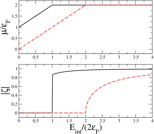
Figure 1: Upper panel: adimensional chemical potential $\mu/\epsilon_{F}$ as a function of the adimensional interaction strength $E_{int}/(2\epsilon_{F})$ for two values of adimensional Rabi energy $E_{\Omega}/(2\epsilon_{F})$: $1/2$ (solid line) and $2$ (dashed line). Lower panel: absolute value $|\zeta|$ of the population imbalance as a function of the adimensional interaction strength $E_{int}/(2\epsilon_{F})$ for the same two values of adimensional Rabi energy $E_{\Omega}/(2\epsilon_{F})$.

The region where $\mu=2\epsilon_{F}$ corresponds to the condition B: the system becomes spin-polarized. In the lower panel of Fig. 1 we plot the population imbalance $|\zeta|$ as a function of the adimensional interaction strength $gn/(2\epsilon_{F})$ for two values of adimensional Rabi energy $E_{\Omega}/(2\epsilon_{F})$. As shown in the figure, the population imbalance $\zeta$, given by Eq. (22), decreases by increasing the Rabi frequency $\Omega$. This result is consistent with previous two-dimensional calculations [34, 35, 36, 37] which suggest, in the absence of Rabi coupling, a jump from $\zeta=0$ to $\zeta=\pm 1$ at the critical strength $g_{c}=4\pi\hbar^{2}/(2m)=E_{kin}/n$. Notice that this jump can be softened also by beyond-mean-field quantum effects [34] or spin-orbit couplings [36]. Our results on the order parameter $\zeta$, and specifically the lower panel of Fig. 1, signal a first-order phase transition if $E_{\Omega}/(2\epsilon_{F})<1$ and a second-order phase transition if $E_{\Omega}/(2\epsilon_{F})>1$.

4 Discussion and inclusion of harmonic confinement

Up to now we have considered a 2D homogeneous fermionic system. Here we discuss the effect of an external hamonic confinement

$$U({\bf r})={1\over 2}m\omega^{2}(x^{2}+y^{2})$$ (32)

on the properties of the 2D system. We adopt the local density approximation [49]:

$${\bar{\mu}}=\mu[n({\bf r})]+U({\bf r})\;,$$ (33)

where ${\bar{\mu}}$ is the chemical potential of the non uniform 2D system, $n({\bf r})=n_{\uparrow}({\bf r})+n_{\downarrow}({\bf r})$ is the local number density with

$$N=\int d^{2}{\bf r}\ n({\bf r})$$ (34)

the total number of fermions, and $\mu[n]$ is the local chemical potential given by Eqs. (30) and (31).

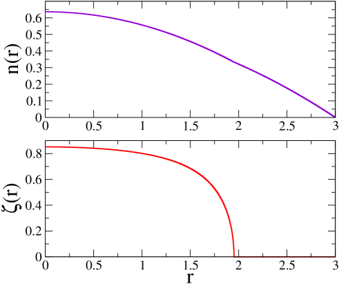
Figure 2: Total density profile $n(r)$ and population imbalance profile $\zeta(r)$ of the 2D Fermi gas under harmonic confinement of frequency $\omega$. We set $\hbar=m=\omega=1$ and choose $\Omega=1$, $g=3$, and $\bar{\mu}=4$. The lower panel shows spin-flip (population imbalance) near the center of the trap while the periphery remains balanced.

By using $r=\sqrt{x^{2}+y^{2}}$ Eq. (33) can be written as

$$r={1\over\omega}\sqrt{2\left(\bar{\mu}-\mu[n]\right)}$$ (35)

which gives the radial coordinate $r$ as a function of the number density $n$. This formula can be easily implemented numerically to determine the density profile $n(r)$, the local population imbalance

$$\zeta(r)=\left\{\begin{array}[]{ll}0&\mbox{ for }n(r)\leq{E_{\Omega}\over g}\\ \sqrt{1-{E^{2}_{\Omega}/(g^{2}n^{2}(r))}}&\mbox{ for }n(r)>{E_{\Omega}\over g}\end{array}\right.\;,$$ (36)

and the local densities of fermions with spin up and spin down:

$$n_{\downarrow}(r)={1\over 2}n(r)\Bigl{(}1+\zeta(r)\Bigr{)}\;,\quad\quad\quad n_{\uparrow}(r)={1\over 2}n(r)\Bigl{(}1-\zeta(r)\Bigr{)}\;.$$ (37)

As an example, in Fig. 2 we report the total number density profile $n(r)$ (upper panel) and the population imbalance profile $\zeta(r)$ (lower panel) with a simple choice of the parameters which ensures that $n(0)>E_{\Omega}/g$. This condition is crucial to produce an atomic cloud with population imbalance. Note that the appearance of a non-zero population imbalance implies a spontaneous symmetry breaking of the ground-state with respect to the choice $\zeta$ or $-\zeta$.

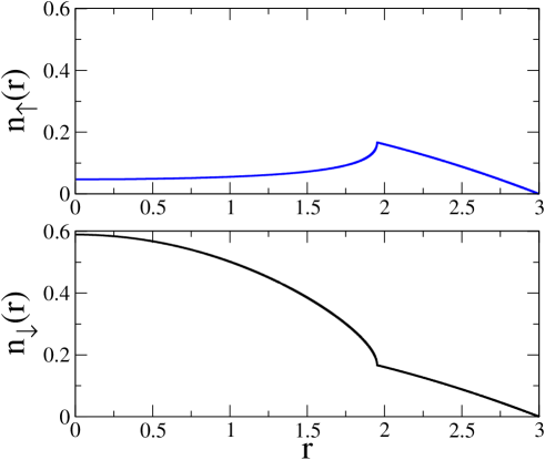
Figure 3: Local densities $n_{\downarrow}(r)$ and $n_{\uparrow}(r)$ of the 2D Fermi gas under harmonic confinement of frequency $\omega$. We set $\hbar=m=\omega=1$ and choose $\Omega=1$, $g=3$, and $\bar{\mu}=4$. The panels clearly show the enhancement of the number of atoms with spin down near the center of the trap, while near the surface the system remains balanced.

In Fig. 3 we plot the corresponding local densities $n_{\downarrow}(r)$ and $n_{\uparrow}(r)$. The figures clearly show that the atomic cloud is characterized by population imbalance near the center of the trap ($r=0$) where the total number density is larger than $E_{\Omega}/g$. Instead, at the periphery (near the surface) of the atomic cloud the gas is fully balanced. We emphasize that setting $\hbar=m=\omega=1$ (as done in Fig. 2 and Fig. 3) amounts to using harmonic-trap units: energies in units of $\hbar\omega$ and lengths in units of $a_{H}=\sqrt{\hbar/(m\omega)}$, that is the characteristic length of harmonic confinement.

In the experiments with ultracold atomic clouds having a quasi-2D disk-shaped configuration on the $(x,y)$ plane, one finds typically $a_{H}\simeq 100$ $\mu$m, while the 2D interaction strength $g$ reads $g=4(\hbar\omega)a_{s}a_{H}^{2}/a_{z}$ with $a_{s}$ the 3D s-wave scattering length and $a_{z}$ the characteristic length of the confinement along the $z$ axis. Remarkably, in current experiments the 3D s-wave scattering length $a_{s}$ can be modified by using an external magnetic field (Fano-Feshbach resonance technique) and consequently one can easily move the system from a weakly-interacting to a strongly-interacting regime.

5 Conclusions

In this paper we have shown how the non-trivial interplay among Pauli exclusion principle, repulsive interaction, and Rabi coupling can induce itinerant ferromagnetism in two-dimensional repulsive Fermi gases. In particular, we have analytically found that for a homogeneous 2D fermionic system there is polarization (i.e., itinerant ferromagnetism) when the interaction energy per particle is larger than both the kinetic energy per particle and the Rabi energy. It is important to stress that the itinerant ferromagnetism is certainly driven by the Stoner instability [32]: a sufficiently large repulsion between fermions make the uniform and balanced system unstable. However, as we have shown in this paper, it is the presence of Rabi coupling that allows the phenomenon of spin flip. In fact, in the absence of Rabi coupling or other spin-dependent mechanisms, the Stoner instability implies phase separation and not spin flip. Similar effects are expected in bosonic mixtures [30, 50]. Here we have adopted a Hartree-Fock mean-field approach. On the basis of previous results obtained in the absence of Rabi coupling in 2D and 3D [43, 45, 51], we expect that beyond-meand-field quantum fluctuations can slightly reduce the critical strength of Stoner instability.

In the last part of the paper we have considered the inclusion of an external harmonic potential, which is the simplest trapping configuration for experiments with ultracold alkali-metal atoms. In this case, we have predicted a remarkable effect we expect to be accessible in the near-future experiments: for a sufficiently large number of fermions, such that the number density at the center of the trap exceeds a critical value, the 2D fermionic gas is characterized by population imbalance near the center of the trap and by a fully balanced configuration near the surface.

References

References

- [1] Lin Y J, Jimenez-Garcia K, and Spielman I B 2011 Nature 471 83
- [2] Zhang J-Y, Ji S-C, Chen Z, Zhang L, Du Z-D, Yan B, Pan G-S, Zhao B, Deng Y-J, Zhai H, Chen S, and Pan J W 2012 Phys. Rev. Lett. 109 115301
- [3] Wang P, Yu Z-Q, Fu Z, Miao J, Huang L, Chai S, Zhai H, and Zhang J 2012 Phys. Rev. Lett. 109 095301
- [4] Cheuk L W, Sommer A T, Hadzibabic Z, Yefsah T, Bakr W S, and Zwierlein M W 2012 Phys. Rev. Lett. 109 095302
- [5] Bychkov Y A and Rashba E I 1984 J. Phys. C 17 6029
- [6] Dresselhaus G 1955 Phys. Rev. 100 580
- [7] Li Y, Pitaevskii L P, and Stringari S 2012 Phys. Rev. Lett. 108 225301
- [8] Martone G I, Li Yun, Pitaevskii L P, and Stringari S 2012 Phys. Rev. A 86 063621
- [9] Burrello M and Trombettoni A 2011 Phys. Rev. A 84 043625
- [10] Merkl M, Jacob A, Zimmer F E, Ohberg P, and Santos L 2010 Phys. Rev. Lett. 104 073603; Fialko O, Brand J, and Zulicke U 2012 Phys. Rev. A 85 051605; Liao R, Huang Z-G, Lin X-M, and Liu W-M 2013 ibid. 87 043605
- [11] Achilleos V, Frantzeskakis D J, Kevrekidis P G, and Pelinovsky D E 2013 Phys. Rev. Lett. 110 264101
- [12] Xu Y, Zhang Y, and Wu B 2013 Phys. Rev. A 87 013614
- [13] Salasnich L and Malomed B A 2013 Phys. Rev. A 87 063625
- [14] Vyasanakere J P and Shenoy V B 2011 Phys. Rev. B 83 094515; Vyasanakere J P, Zhang S, and Shenoy V B 2011 Phys. Rev. B 84 014512
- [15] Gong M, Tewari S, and Zhang C 2011 Phys. Rev. Lett. 107 195303
- [16] Hu H, Jiang L, Liu X-J, and Pu H 2011 Phys. Rev. Lett. 107 195304
- [17] Iskin M and Subasi A L 2011 Phys. Rev. Lett. 107 050402
- [18] Dell’Anna L, Mazzarella G, and Salasnich L 2011 Phys. Rev. A 84 033633; Dell’Anna L, Mazzarella G, and Salasnich L 2012 Phys. Rev. A 86 053632
- [19] Han Li and Sa de Melo C A R 2012 Phys. Rev. A 85 011606(R)
- [20] Chen G, Gong M, and Zhang C 2012 Phys. Rev. A 85 013601
- [21] Zhou K, Zhang Z 2012 Phys. Rev. Lett. 108 025301
- [22] Yang X, Wan S 2012 Phys. Rev. A 85 023633
- [23] Salasnich L 2013 Phys. Rev. A 88 055601
- [24] Gigli L and Toigo F 2015 J. Phys. B: At. Mol. Opt. Phys. 48 245302
- [25] Loktev V M, Quick R M, and Sharapov S G 2001 Phys. Rep. 349 1
- [26] Ando T, Fowler A B, and Stern F 1982 Rev. Mod. Phys. 54 437; Mannhart J, Blank D H A, Hwang H Y, Millis A J, and Triscone J-M 2008 MRS Bull. 33 1027
- [27] Lewenstein M, Sanpera A, and Ahufinger V 2012 Ultracold atoms in optical lattices: simulating quantum many-body systems (Oxford: Oxford University Press).
- [28] Steck D A, Quantum and Atom Optics, available online at http://steck.us/teaching.
- [29] Horstmann B, Durr S, and Roscilde T 2010 Phys. Rev. Lett. 105 160402
- [30] Nicklas E, Strobel H, Zibold T, Gross C, Malomed B A, Kevrekidis P G, and Oberthaler M K 2011 Phys. Rev. Lett. 107, 193001
- [31] Jo G-B, Lee Y-R, Choi J-H, Christensen C A, Kim T H, Thywissen J H, Pritchard D E, and Ketterle W 2009 Science 325 1521–152
- [32] Stoner E C 1947 Rep. Prog. Phys. 11 43
- [33] Salasnich L, Pozzi B, Parola A, and Reatto L 2000 J. Phys. B 33 3943
- [34] Conduit G J, Green A G, and Simons B D 2009 Phys. Rev. Lett. 103 207201
- [35] Massignan P, Yu Z, and Bruun G M 2013 Phys. Rev. Lett. 110, 230401 (2013).
- [36] Ambrosetti A, Lombardi G, Salasnich L, Silvestrelli P L, and Toigo F 2014 Phys. Rev. A 90 043614
- [37] Jiang Y, Kurlov D V, Guan Xi-W, Schreck F, Shlyapnikov G V 2016 Phys. Rev. A 94, 011601(R) (2016).
- [38] Sanner C, Su E J, Huang W, Kesher A, Gillen J, and Ketterle W 2012 Phys. Rev. Lett. 108 240404
- [39] Petrov D S and Shlyapnikov G V, 2001 Phys. Rev. A 64 012706
- [40] Massignan P, Zaccanti M and Bruun G M 2014 Rep. Prog. Phys. 77 034401
- [41] Valtolina G, Scazza F, Amico A, Burchianti A, Recati A, Enss T, Inguscio M, Zaccanti M, and Roati G 2016 arXiv:1605.07850
- [42] Salasnich L and Toigo F 2008 J. Low Temp. Phys. 150 643; Mazzarella G, Salasnich L and Toigo F 2009 Phys. Rev. A 79 023615
- [43] Conduit G J 2010 Phys. Rev. A 82 043604
- [44] He L Y and Huang X G 2012 Phys. Rev. A 85 043624
- [45] Conduit G J 2013 Phys. Rev. B 87 184414
- [46] van Oosten D, van der Straten P, and Stoof H T C 2001 Phys. Rev. A 63 053601
- [47] Buonsante P, Penna V, and Vezzani A 2005 Laser Phys. 15 361
- [48] Penna V and Raffa F A 2014 J. Phys. B: At. Mol. Opt. Phys. 47 075501
- [49] Lipparini E 2008 Modern many-particle physics (Singapore: World Scientific)
- [50] Lingua F, Guglielmino M, Penna V, and Capogrosso-Sansone B 2015 Phys. Rev. A 92 053610
- [51] Pilati S, Bertaina G, Giorgini S, and Troyer M 2010 Phys. Rev. Lett. 105 030405