Tracking random walks

Abstract

In empirical studies of random walks, continuous trajectories of animals or individuals are usually sampled over a finite number of points in space and time. It is however unclear how this partial observation affects the measured statistical properties of the walk, and we use here analytical and numerical methods of statistical physics to study the effects of sampling in movements alternating rests and moves of random durations. We evaluate how the statistical properties estimated are affected by the way trajectories are measured and we identify an optimal sampling frequency leading to the best possible measure. We solve analytically the simplest scenario of a constant sampling interval and short-tailed distributions of rest and move durations, which allows us to show that the measured displacement statistics can be significantly different from the original ones and also to determine the optimal sampling time. The corresponding optimal fraction of correctly sampled movements, analytically predicted for this short-tail scenario, is an upper bound for the quality of a trajectory’s sampling. Indeed, we show with numerical simulations that this fraction is dramatically reduced in any real-world case where we observe long-tailed distributions of rest duration. We test our results with high resolution GPS human trajectories, where a constant sampling interval allows to recover at best $18\%$ of the movements, while over-evaluating the average trip length by a factor of $2$. If we use a sampling interval extracted from real communication data, we recover only $11\%$ of moves, a value that cannot be increased above $16\%$ even with ideal algorithms. These figures call for a more cautious use of data in all quantitative studies of individuals’ trajectories, casting in particular serious doubts on the results of previous studies on human mobility based on mobile phone data.

The recent years have witnessed a dramatic increase in the use of large amounts of data available thanks to Information and Communication Technologies. These new sources allow to monitor and to map the dynamical properties of many complex systems at an unprecedented scale Vespignani:2012 and we have now access to a vast number of spatial trajectories representing movements of objects in geographical space Zheng:2015 . In particular, such datasets have opened the opportunity to better understand human movements Gonzalez:2008 ; Song:2010mod ; Raichlen:2014 ; Gallotti:2015ttb ; Gallotti:2016acc and the impact of mobility on important processes such as epidemic spreading Balcan:2009 . These recent works extend previous studies of movements and foraging patterns of animals Book:foraging ; Reynolds:2015 and rely on tracking man-made inanimate objects Brockmann:2006 ; Phithakkitnukoon:2013 . However, as it is the case for any dataset, these new sources of information have limits and biases Cagnacci:2010 ; Sagarra:2015 ; Williams:2015 ; Colak:2016ana that need to be assessed.

It is common to approximate the continuous spatio-temporal record of the followed individual (or animal) by a series of straight lines, thus describing the movements of an organism as a sequence of behavioural events called moves for animals Book:Turchin and trips for humans. This empirical approach allows a natural implementation of the theoretical framework of continuous-time random walks Brockmann:2006 ; Codling:2008 , where a rest time is associated to the endpoint of each move. However, this leads to the first major problem due to the lack of behavioural information in the empirical data Hebbiewhite:2010 . Real trajectories always exhibit a large variety of intertwined static and dynamic behaviours Laube:2011 : slow versus fast movement behaviour for animals Hebbiewhite:2010 , fixation versus saccade in eye-tracking Salvucci:2000 , or activities versus trips in human mobility Kitamura:1997 . Isolating and identifying these behaviours from a series of chronologically ordered points is an important statistical challenge Fryxell:2008 and a growing array of methods based on spatio-temporal characteristics of the trajectories have been developed to perform this task automatically Salvucci:2000 ; Hebbiewhite:2010 ; Zheng:2015 . These methods are however often tailored for the specific dataset in question Laube:2011 . Therefore, even the working definition of a ‘move’ might vary significantly between studies, depending on the method and the technology used Edwards:2011 .

A second complication comes from the limits of the technology used for collecting the empirical data. In the case of spatial movements, a crucial aspect is the temporal sampling of the trajectory. The simplest and most common method used is to record the spatial coordinates at regular intervals, and to associate the observed displacements to continuous moves Book:Turchin . However, this is a strong oversimplification, and all derived quantities will depend on the sampling process itself Codling:2005 ; Laube:2011 ; Rosser:2013 . The random sampling of random processes might even be the principal cause of the emergence of long tails in several statistical distributions Reed:2002 ; Mosetti:2007 . For example, in the case of movement in space that we will study in this paper, it has been shown that non-Lévy movements can be erroneously interpreted as Lévy flights when sampling time intervals are larger than the natural time scale of animals’ movements Plank:2009 ; Codling:2011 . The sampling rate is thus a crucial element that has to be taken into account when analyzing empirical trajectories Laube:2011 .

Currently, the most common sources of human mobility data are Call Detail Records (CDR) of mobile phone data Blondel:2015 and geo-located social media accesses Hawelka:2014 . Both suffer from the flaws described above. Indeed, in these data, trajectories are represented as sequences of positions recorded at the moment of an event (which can be a call, a text message or an application access). The trajectory sampling is therefore coupled to the random and bursty nature of human communications Barabasi:2005 . The probability distribution of the time interval between calls Gonzalez:2008 ; Song:2010mod , e-mails Barabasi:2005 and tweets Bild:2015 has a long tail which can be fitted by a power law with an exponent value close to $-1$ (and with a cutoff of the order of days). Only in a few cases, a small set of trajectories sampled every $\Delta=1$ or $2$ hours is available Gonzalez:2008 ; Song:2010mod ; Song:2010lim .

The nature of data forces therefore researchers to make (implicitly or not) the following naive assumptions:

• An individual is always at rest at the location where there is a communication event (call, sms).

• Every change of position is associated to a single move.

This point of view has been adopted in the first important papers where human mobility has been studied with mobile phone data Gonzalez:2008 ; Song:2010mod and often replicated, even in recent studies Pappalardo:2015 ; Barbosa:2015 ; Pappalardo:2016b . Even when individuals with a very high call frequency are selected Song:2010lim , they are still inactive most of the time Bagrow:2012 . In order to identify human mobility patterns, it thus became necessary to introduce ad-hoc methods based on reasonable assumptions and almost arbitrary parameters Jiang:2013 ; Colak:2016ana .

In this paper we discuss the effect of sampling and assumptions $(i)$ and $(ii)$ on the measured properties of random movements. We will consider one of the simplest and realistic cases where the trajectory consists of two alternating phases, moves and rests, whose durations $t$ and $\tau$ are regarded as independent random variables. Trajectories can then be seen as an alternating renewal process, i.e., a generalisation of Poisson processes to arbitrary holding times and to two alternating kinds of events. The sampling time interval $\Delta$ depends on the particular experiment and can be either constant or randomly distributed. Using methods of renewal theory along the lines of Godreche:2001 , we provide a theoretical estimate for the fraction of correctly sampled trips with a constant sampling interval, and show the existence of an optimal sampling. We then extend these results numerically, and show that sampling human trajectories in more realistic settings is necessarily worse. Finally, we use high-resolution (spatially and temporally) GPS trajectories to verify our predictions on real data.

I Results

I.1 Theoretical analysis

We study the effect of the sampling rate on the apparent distribution of move lengths that is measured. We focus on the case of an alternating sequence of rests and moves and we further assume that the movement is one-dimensional with a constant velocity $v$ (see SI for other cases). In particular, we will not discuss the apparent speed and turning angles in a general two-dimensional case Codling:2005 ; Laube:2011 ; Rosser:2013 , the possible fits of the displacement distribution Reynolds:2008 ; Benhamou:2008 ; Plank:2009 ; Codling:2011 , or interpolation methods to reconstruct the movements between samplings Hoteit:2014 . The quantities entering this problem are therefore: the move duration $t$, the move length $\ell=vt$, the resting time $\tau$, and the time interval $\Delta$ between two consecutive measures. The distributions $P(t)$ and $P(\tau)$ are characteristic of the specific subject in motion, while the distribution of the sampling interval $P(\Delta)$ is associated to the technology used for tracking the motion. Sampling the trajectory gives us a displacement distribution $P(\ell^{\ast})$ where $\ell^{\ast}$ is the apparent length of a move, and the problem is thus to compute this distribution $P(\ell^{\ast})$ for any given distributions $P(t)$, $P(\tau)$, and $P(\Delta)$.

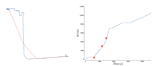
Figure S1: Representing trajectories. (Left) Trajectory obtained with GPS readings (solid blue) and sampled trajectory (dashed red). (Right) Cumulated distance traveled on the real trajectory (solid blue) and sampling points (red crosses) drawn from a power-law distribution with exponent $-1$. The sampled trajectory is a gross approximation of the real trajectory, a lot of information being lost in the process.

During rests, the displacement is assumed to be zero, and so the succession of rests and moves is associated to a continuous increasing function $x(\theta)$, where $\theta$ is the time parameter (see Fig. 1). We sample the position $x^{\ast}_{k}$ for every instant $\theta^{\ast}_{k}=\sum_{j=1}^{k}\Delta_{j}$, where $\Delta_{j}$ is the $j$th value of the sampling interval (in the case of constant sampling, $\Delta_{j}=\overline{\Delta}$, and so $\theta^{\ast}_{k}=k\overline{\Delta}$). The succession of space-time coordinates $(\theta^{\ast}_{k},x^{\ast}_{k})$ (shown in Fig. 1 and in the 2D example of Fig. S1) thus represents all the knowledge we have about the trajectory after sampling. For two consecutive measures at times $\theta^{\ast}_{k}$ and $\theta^{\ast}_{k+1}$ there is an observed displacement $\ell^{\ast}_{k}=x^{\ast}_{k+1}-x^{\ast}_{k}$. Our goal is then to estimate the differences between the distribution of real displacement lengths $\ell$ and of the observed displacements $\ell^{\ast}_{k}$. In particular, we want to understand the biases induced by different choices for $P(\Delta)$.

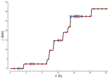
Figure 1: Examples of trajectory sampling. On a trajectory with exponentially distributed rest and move durations, we show the case of constant sampling interval (red circles) and the case of random sampling interval (blue crosses) with $P(\Delta)\propto\Delta^{-1}$ ($\Delta_{\rm min}=5$ min, $\Delta_{\rm max}=12$ h). See Fig. S1 for a 2D example.

If we make the naive assumption, discussed in the introduction, that every observed displacement is associated to a single move, the necessary condition for this to be correct is that two subsequent sampling times $\theta^{\ast}_{k}$ and $\theta^{\ast}_{k+1}$ fall in two consecutive rests. We can also easily identify the cases where the sampling times fall in the same rest, since this is the only situation where we exactly have $\ell^{\ast}_{k}=0$ and which does not lead to a wrong estimate of the individual’s movement. Conversely, we must consider as errors all other configurations, since they lead to a mis-interpretation of the individual mobility and to an under- or over-estimate of the move lengths Plank:2009 and of the number of trips observed Williams:2015 . In order to go beyond this simple hand-waving argument, we will consider the case of exponential distributions for $P(t)$ and $P(\tau)$, constant sampling time interval $\overline{\Delta}$, and constant speed $v$. In this case we obtain explicitly the distribution $P(\ell^{\ast})$ of sampled displacements. This will allow us to discuss the impact of the sampling, and to show in particular that there is an optimal value for $\overline{\Delta}$.

I.1.1 Constant sampling rate and exponential distributions

We will consider the case of exponential distributions for the move and rest durations:

$$P(t)=(1/\overline{t})\,\exp(-t/\overline{t}),\;\;P(\tau)=(1/\overline{\tau})\,\exp(-\tau/\overline{\tau})$$ (1)

and a constant sampling interval:

$$P(\Delta)=\delta(\Delta-\overline{\Delta})$$ (2)

($\delta(x)$ is Dirac’s delta function). In the constant velocity case, the real displacements are also exponentially distributed:

$$P(\ell)=(1/\overline{\ell})\,\exp(-\ell/\overline{\ell}),$$ (3)

with $\overline{\ell}=v\overline{t}$.

Using methods of renewal theory feller ; cox ; coxm , along the lines of Godreche:2001 , we obtain an explicit expression for the distribution $P(\ell^{\ast})$ (see Eqs. (S17), (S35)):

$$P(\ell^{\ast})=\frac{{\rm e}^{-\overline{\Delta}/\overline{\tau}}}{1+\overline{t}/\overline{\tau}}\delta(\ell^{\ast})+\frac{{\rm e}^{-\overline{\Delta}/\overline{t}}}{1+\overline{\tau}/\overline{t}}\delta(\ell^{\ast}-v\overline{\Delta})+P_{\rm cont}(\ell^{\ast})\,,$$ (4)

where the continuous part of this distribution reads

$$P_{\rm cont}(\ell^{\ast})=\frac{2{\rm e}^{-\left(\frac{\ell^{\ast}}{v\overline{t}}-\frac{v\overline{\Delta}-\ell^{\ast}}{v\overline{\tau}}\right)}}{v(\overline{t}+\overline{\tau})}\!\left[\!I_{0}(y)+\!\left(\!\frac{\ell^{\ast}}{v\overline{\tau}}+\frac{v\overline{\Delta}-\ell^{\ast}}{v\overline{t}}\!\right)\!\frac{I_{1}(y)}{y}\!\right]\!,$$ (5)

with $y=2\sqrt{\frac{\ell^{\ast}(v\overline{\Delta}-\ell^{\ast})}{v^{2}\overline{t}\overline{\tau}}}$, and where $I_{0}(y)$ and $I_{1}(y)$ are modified Bessel functions of the first kind.

In the following we will not consider the discrete part $\delta(\ell^{\ast})$ of the distribution $P(\ell^{\ast})$, since the value $\ell^{\ast}=0$ can be easily recognized and excluded in any practical scenario. The fraction of sampling intervals associated to null movements ($\ell^{*}=0$), denoted by $C_{0}(\overline{\Delta})$, can be significantly large. In the stationary regimemetzler , we can compute $C_{0}(\overline{\Delta})$ for any distributions $P(t)$ and $P(\tau)$, and a constant sampling time $\overline{\Delta}$ (see Eq. (S19)). We can show that it is a decreasing function, varying between $C_{0}(0)=\overline{\tau}/(\overline{t}+\overline{\tau})$ (i.e., the fraction of time spent at rest, in the continuous sampling limit) and $C_{0}(\infty)=0$. In the particular case of exponential distributions (Eq. (1)), $C_{0}$ is the prefactor of the $\delta(\ell^{\ast})$ peak in Eq. (4), and can be very large. For instance, $C_{0}\approx 60\%$ in the case of car mobility ($\overline{t}=0.30$ h and $\overline{\tau}=2.49$ h, see SI) and $\overline{\Delta}=1$ h. For this reason, we compare the original data to a rescaled probability distribution which does not include the $\delta(\ell^{\ast})$ peak and is given by (see Fig. S4)

$$P_{\ell^{\ast}>0}(\ell^{\ast})=\frac{1}{1-C_{0}(\overline{\Delta})}\left[\frac{{\rm e}^{-\overline{\Delta}/\overline{t}}}{1+\overline{\tau}/\overline{t}}\delta(\ell^{\ast}-\overline{\Delta})+P_{\rm cont}(\ell^{\ast})\right].$$ (6)

We show in Fig. 2 (top) the dependence of the continuous part of $P_{\ell^{\ast}>0}(\ell^{\ast})$ on $\overline{\tau}$, keeping the average travel time $\overline{t}$ fixed to the experimental value of $0.30$ h for car mobility Gallotti:2016acc .

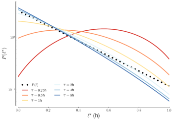
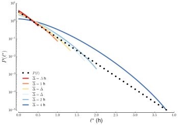
Figure 2: Distributions $P(\ell^{*})$ obtained from sampling. (Top) Dependence of Eq. (6) on $\overline{\tau}$ fixing $\overline{t}=0.30$ h and $\overline{\Delta}$ = 1 h. (We choose here $v=1$). The distribution has a maximum when the average rest times exceeds the sampling time. (Bottom) Dependence of Eq. (6) on $\overline{\Delta}$ fixing $\overline{t}=0.30$ h, $\overline{\tau}=2.49$ h. Short sampling times introduce a cut-off in the distribution. Large fluctuations can be observed when sampling time intervals are long.

We note that $P_{\rm cont}(\ell^{\ast})$ can have a maximum, even if the original distribution $P(\ell)$ is a decreasing function. The measurements allow us to recover the exponential tail of travel times only if the resting time $\overline{\tau}$ is sufficiently long. Conversely, when the sampling time $\overline{\Delta}$ is larger than the average duration of a rest, the result of the sampling is manifestly different from the original exponential distribution. In Fig. 2 (bottom), we take $\overline{t}=0.30$ h and $\overline{\tau}=2.49$ h (which are the values observed for vehicular mobility, see SI) and study the outcome for different sampling times $\overline{\Delta}<\overline{\tau}$. Naturally, $\overline{\Delta}$ acts as a cutoff since all moves longer than this value are necessarily interrupted by the sampling. In contrast, for large values of $\overline{\Delta}$, the number of short travels is under-estimated, since subsequent short moves may be joined together and thus appear as an effective long one.

We also computed exactly the first two moments of the distribution Eq. (4) and found for the average

$$\langle\ell^{\ast}\rangle=\frac{v\overline{\Delta}}{1+\overline{\tau}/\overline{t}}$$ (7)

(see Eq. (S29), and Eq. (S30) for the second moment). Naturally, the exclusion of the null displacements influences the value of the distribution’s moments. In particular, the average value of Eq. (6) can be computed by a simple rescaling and reads

$$\langle\ell^{\ast}\rangle_{\ell^{\ast}>0}=\frac{\langle\ell^{\ast}\rangle}{1-C_{0}(\overline{\Delta})}.$$ (8)

This rescaling yields notable changes in the numerical values of the moments. For instance, with realistic values for car mobility ($\overline{t}=0.30$ h and $\overline{\tau}=2.49$ h), a sampling time of $1$ h gives $\langle\ell^{\ast}\rangle/v\approx 0.11$ h, while excluding the zero-displacement part we obtain $\langle\ell^{\ast}\rangle_{\ell^{\ast}>0}/v\approx 0.27$ h.

I.1.2 Optimal sampling times

We first note that high-frequency sampling ($\Delta\to 0$) does not automatically allow to understand the whole trajectories. Indeed, it is only with additional data that we can correctly reconstruct a whole trajectory. It is then necessary to implement a ‘segmentation’ algorithm that goes beyond the assumption $(ii)$ that an observed displacement corresponds to one single move, as $\Delta\to 0$ implies that any move is cut in a very large number of segments Book:Turchin . In addition, high-frequency recordings are known to present uncertainties and systematic errors that need to be taken into account for extracting meaningful information Book:Turchin ; Giannotti:2007 ; Wang:2010 ; Laube:2011 ; Ranacher:2016 . A good segmentation algorithm should take into account the noise, the spatial scale, and characteristic speeds of the tracked subjects. Here, it is not our intent to develop detailed segmentation methods, but to show the quality, and the limits, of the simpler assumption that one observed displacement is equal to one move. In this framework, having $\Delta\to 0$ means that we measure moves over a very short time, obtaining thus a distribution of measured displacement peaked at very small values.

We can define an ‘optimal constant sampling time’ in two different ways: either as the time interval $\mathring{\Delta}$ that correctly estimates the average length of moves, or as the time interval $\hat{\Delta}$ that maximizes the fraction of correctly sampled moves. In the following, we obtain exact formulas for both $\mathring{\Delta}$ and $\hat{\Delta}$ in the peaked case (i.e., with conditions described by Eq. (1)).

I.1.3 Average move duration and total number of moves

The optimal sampling time $\mathring{\Delta}$ can be obtained by solving for $\overline{\Delta}$ the equation $\langle\ell^{\ast}\rangle_{\ell^{\ast}>0}=v\overline{t}$. The solution can be written in the form

$$\mathring{\Delta}=\overline{\tau}\,W(-{\rm e}^{-\overline{t}/\overline{\tau}-1})+\overline{t}+\overline{\tau}\,,$$ (9)

where $W(x)$ is the Lambert function, such that $W(x){\rm e}^{W(x)}=x$. This function is defined for $x\geq-{\rm e}^{-1}$, which always holds in our case since $\overline{t},\overline{\tau}>0$. Using the empirical values $\overline{t}=0.30$ h, $\overline{\tau}=2.49$ h we obtain $\mathring{\Delta}\approx 80$ min. This result is confirmed by Monte-Carlo simulations (Fig. 3), where red circles represent the values for $\mathring{\Delta}$. With this ‘optimal’ sampling time based on the first moment, the second moment is slightly under-estimated. Note that matching the average travel time is equivalent to correctly estimating the number $n$ of trips, i.e., of moves and stops (see inset in Fig. 3 (top)). For $\overline{\Delta}>\mathring{\Delta}$ the trajectory is under-sampled ($n^{\ast}<n$) and trip lengths over-estimated, while for $\overline{\Delta}<\mathring{\Delta}$ it is over-sampled ($n^{\ast}>n$) and trip lengths are under-estimated.

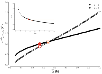
Figure 3: Optimal sampling for exponential distributions and constant sampling. (Top) First ($k=1$) and second ($k=2$) moment of displacement (normalized by $\langle\ell\rangle$ and $\langle\ell^{2}\rangle$, respectively) versus sampling time interval. The original average value $\langle\ell\rangle$ (yellow solid line) is obtained by definition for $\overline{\Delta}=\mathring{\Delta}$ (filled circle), while is over-estimated by $\approx 10\%$ for $\overline{\Delta}=\hat{\Delta}$ (up triangle). The second moment ($k=2$) has a deviation of about $10\%$ for both optimal sampling times (empty circle and down triangle). In the inset, we show the ratio of the estimated number of trips $n^{*}$ over the actual number of trips $n$. With $\overline{\Delta}=\mathring{\Delta}$ (circle) we correctly evaluate the number of moves, while $\overline{\Delta}=\mathring{\Delta}$ (triangle) yields to a slightly under-estimated value $n^{\ast}\approx 0.90n$. (Bottom) The fraction of good moves follows the curve predicted by Eq. (10) (blue line). The maximum value of $51\%$ is reached for $\overline{\Delta}=\hat{\Delta}$ (triangle), but at $\overline{\Delta}=\mathring{\Delta}$ (circle) the value is only $1\%$ lower. We choose here $\overline{t}=0.30$ h, $\overline{\tau}=2.49$ h.

This point of view about the number of moves allows us to extend the validity of this optimal sampling to higher dimensionality (2D or 3D) and to any distribution $P(v)$. The dimensionality of space indeed does not influence the moves’ number counting. To illustrate this, we extend this analysis in the SI with a Monte-Carlo simulation in the case where speed is a random variable dependent on the move duration Gallotti:2016acc . In this case, our exact results for $P(\ell)$ do not hold anymore, because moves have different speeds. Nevertheless, the value given by Eq. (9) only under-estimates the mean displacement length with varying speeds by some $5\%$.

I.1.4 Fraction of correctly sampled moves

In order to estimate $\hat{\Delta}$, we have to compute the fraction $F_{\rm good}$ of movements that are correctly measured. This occurs when two consecutive sampling times fall during the rests immediately before and after a move, say $\theta^{\ast}_{k}$ in the rest $\tau_{m}$ and $\theta^{\ast}_{k+1}=\theta^{\ast}_{k}+\overline{\Delta}$ in the rest $\tau_{m+1}$. The probability $P_{\rm good}$ of the latter event and the fraction $F_{\rm good}=P_{\rm good}/(1-C_{0})$ are calculated in the SI. In the case of exponential distributions, we obtain the explicit expression (see Eq. (S39))

$$F_{\rm good}(\overline{\Delta})=\frac{\overline{t}\overline{\tau}}{(\overline{\tau}-\overline{t})^{2}}\frac{{\rm e}^{-\overline{\Delta}/\overline{t}}+\left(\frac{(\overline{\tau}-\overline{t})\overline{\Delta}}{\overline{t}\overline{\tau}}-1\right){\rm e}^{-\overline{\Delta}/\overline{\tau}}}{1+\overline{t}/\overline{\tau}-{\rm e}^{-\overline{\Delta}/\overline{\tau}}}\,.$$ (10)

In Fig. 3 (bottom) we compare the shape of $F_{\rm good}$ for fixed values of $\overline{t}$ and $\overline{\tau}$ with the result of a Monte-Carlo simulation. For empirical values valid for car mobility ($\overline{t}=0.30$ h, $\overline{\tau}=2.49$ h), the curve has a maximum $\hat{F}_{\rm good}\approx 51\%$ for a sampling time given by $\hat{\Delta}=1.70$ h (102 min). Both the value of $\hat{\Delta}$ and the height $\hat{F}_{\rm good}$ of the maximum of $F_{\rm good}(\overline{\Delta})$ depend on the ratio $\overline{t}/\overline{\tau}$ (see Fig. S2). They are however independent of the spatial embedding and of the characteristics of $P(v)$. The quantity $\hat{F}_{\rm good}\approx 51\%$ is associated with the largest value of $\overline{\tau}$ for the data sources we have analyzed (mobile data, GPS trajectories, and car mobility, see SI), and thus represents the best possible value associated to human mobility. It is remarkable that the optimal fraction $\hat{F}_{\rm good}$ of sampled movements in human mobility is so low that essentially one half of the moves at cut or merged during the sampling, limiting the possibility of understanding the individuals’ behaviour. We also note that the value $F_{\rm good}(\mathring{\Delta})$ is not far from $51\%$ (Fig. 3 (bottom)). We thus see that, even if the measured and the real distributions are similar with comparable first moments, we are often describing different movements. The nature of the process, characterized by $\overline{\tau}$ and $\overline{t}$, limits our knowledge of the system for any value of $\overline{\Delta}$.

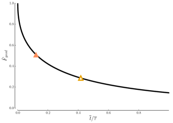
Figure 4: Maximization of $F_{\rm good}$. (Top) The maximum $\hat{F}_{\rm good}$ for exponential distributions. We observe that $\hat{F}_{\rm good}\to 1$ in the limit for small $\overline{t}$, and decreases as $\overline{t}$ becomes comparable to $\overline{\tau}$. The upper bound to sampling quality is $51\%$ for the car mobility conditions of Fig. 3 (orange solid triangle) and $29\%$ for GeoLife trajectories of Fig. 5 (yellow empty triangle). (Bottom) The sampling rate $\hat{\Delta}$ optimizing $F_{\rm good}$ has a non-trivial dependence on $\overline{t}$ and $\overline{\tau}$. We identify a relatively weak dependence on $\overline{t}/\overline{\tau}$, of the form $\hat{\Delta}=\alpha\sqrt{\overline{t}\overline{\tau}}$, with $\alpha$ ranging between $1.84$ and $2$ for all values of $\overline{t}<\overline{\tau}$. In particular, for the characteristic values observed for car mobility (orange solid triangle, $\overline{t}=0.30$ h, $\overline{\tau}=2.49$ h), the curve exhibits a plateau, allowing us to approximate $\hat{\Delta}\approx 1.96\sqrt{\overline{t}\overline{\tau}}$. For the GeoLife trajectories (yellow empty triangle), which have significantly shorter rest times ($\overline{t}=0.33$ h, $\overline{\tau}=0.80$) the deviation from this approximation is only of about $1.5\%$.

The maximal value $\hat{F}_{\rm good}$ is naturally associated to a second optimal sampling time, which is of the same order as $\overline{t}$ and $\overline{\tau}$: $\hat{\Delta}=\alpha\sqrt{\overline{t}\overline{\tau}}$. The function $\alpha(\overline{t}/\overline{\tau})$ can approximated as a constant (see Fig. 4):

$$\hat{\Delta}=1.96\sqrt{\overline{t}\overline{\tau}}.$$ (11)

This result suggests that the sampling with $\overline{\Delta}\ll\overline{t},\overline{\tau}$ is not optimal and will lead to incorrect results. Such a high-frequency sampling is useful only when we have additional information that allows to reconstruct the trajectory.

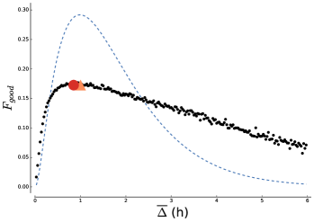
Figure 5: Constant sampling on GPS data. Results are obtained by sampling the GeoLife GPS data with a constant sampling interval $\Delta$. We show (black dots) the fraction of moves correctly sampled as a function of the length of the sampling interval $\overline{\Delta}$. In dashed blue, the theoretical curve computed in ideal conditions. The red circle corresponds to $\mathring{\Delta}=52$ min, while orange triangles correspond to the theoretical maximum $\hat{\Delta}=1$ h of $F_{\rm good}$. Strikingly, the latter coincides with the empirical value of $\hat{\Delta}$.

I.2 Sampling human movements

The conditions of Eqs. (1), (2) define a process where both travel and rest times have a short-tailed distribution and the trajectory sampling is strictly periodic. While this allowed us to find exact analytical expressions and to uncover important effects of sampling on the statistical properties of trajectories, real-world problems are much more involved. Indeed, human travel times are characterized by short-tailed distributions (see Gallotti:2016acc and references therein), and resting time can be broadly distributed for both humans Song:2010mod ; Gallotti:2012 or animals (see Poekt:2012 and references therein). In addition, the trajectory can be sampled with a random inter-sampling time.

We show here that the peaked conditions discussed above correspond in fact to the best-case scenario. In particular, when rests or sampling times are broadly distributed, the outcome of the sampling will be necessarily worse. We first confirm with Monte-Carlo simulations the validity for more complex cases of the results obtained above for a constant sampling time interval. In particular, we show (see SI and Table S1 for details) how the sampling quality $F_{\rm good}$ for cars’ mobility progressively decreases from the upper bound of $51\%$ when introducing randomness in sampling times (exponential or power-law) and in rest durations. For instance, introducing a broad $P(\tau)$ yields to values of $F_{\rm good}$ lower than $40\%$, while a broad $P(\Delta)$ yields to an $F_{\rm good}$ lower than $30\%$. We finally predict that, when coupling a broad $P(\Delta)$ and a broad $P(\tau)$ (as observed for mobile phone data), the quality of the sampling decrease significantly, with $F_{\rm good}$ falling to $23\%$.

We illustrate these different results on a spatio-temporal high-resolution dataset, namely the GeoLife GPS trajectories Geolife3 ; Zhao:2015 . The data consist of coordinates given every $5$ seconds, thus allowing us to perform a speed-based sequencing (see SI). We measure the properties of the sequenced trajectories and find again an average trip time $\overline{t}\approx 0.33$ h. The average rest time drops to $\overline{\tau}\approx 0.8$ h, because data allow us to define activities at a finer scale. Using the functional form for $F_{\rm good}$ given by Eq. (10) for the ideal case, we find that the upper bound for the sampling quality drops consequently to $\hat{F}_{\rm good}=29\%$. In the following, we use these GeoLife GPS trajectories to study the effect of sampling on real trajectories. In particular, we will validate the previous results by studying the effect of constant sampling and then use mobile phone data to sample the GPS trajectories with a random sampling interval.

We first sample the trajectories with a constant time interval $\overline{\Delta}$ that varies between $1$ minute and $6$ hours. For each value of $\overline{\Delta}$, we compute the fraction of the trips that are correctly identified. The results are represented in Fig. 5. They confirm our analytical predictions. Indeed, we find that there exists an optimum value of the sampling time $\overline{\Delta}_{\rm opt}\approx 60$ min. Even though this was not expected, because of a non-exponential $P(\tau)$, this value coincides with the predicted maximum $\hat{\Delta}\approx 1.96\sqrt{\overline{t}\,\overline{\tau}}\approx 60$ min (the theoretical curve is represented as a dashed line on Fig. 5). The fraction of correctly sampled moves is lower than in the idealized case with at best $18\%$ of the trips that are recovered ($F_{\rm good}\approx 0.18$) with a constant sampling interval.

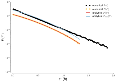
Figure S3: Rescaled distribution of travel times. Optimal Sampling of $\overline{t}=0.30$ h with $\overline{\Delta}=\hat{\Delta}=1.73$ h. The distribution of sampled travel times (light blue) can be compared with the original exponential distribution (black dots) after re-normalizing the distribution, multiplying it by the factor $(1-C_{0})^{-1}$.

We also estimate the average length of the sampled trips for every value of the sampling interval and compare it to the average trip length in the original sequenced trajectory (results are represented in Fig. S3). The optimal value of the sampling time $\overline{\Delta}\approx 15$ min is much smaller than the one maximizing the number of correctly sampled trips. Furthermore we find that, at the optimal sampling interval $\overline{\Delta}\approx 60$ min, the average sampled trip 2D displacement is about $2$ times larger than the average trip length of the original trajectories.

In the case of geolocalized data obtained from devices such as mobile phones, position and time are recorded at random times corresponding to a call or another event. The sampling time intervals are thus random variables. In general they are distributed according to a broad law such as a power-law with exponent close to $-1$ Gonzalez:2008 ; Song:2010mod . Here we use CDR mobile phone data from Senegal DeMontjoye:2014 and, as commonly done Song:2010lim ; Pappalardo:2015 , extract the duration between calls of the users with extremely high average call frequency, in the same spirit as in Gonzalez:2008 . We then sample the sequenced GPS trajectory using these durations. The result is staggering: only $11\%$ of the trips are correctly sampled. One may argue that calls and rests are correlated, or that calls done during moves can be filtered out. We thus computed the proportion of correctly sampled trips at different levels of correlation (see SI for details), and find that, at best—when we only have calls during rests—only $16\%$ of trips are recovered. The use of CDR mobile phone data or of any dataset presenting a largely distributed inter-event time to study mobility is thus very questionable. We note that forcing a perfect correlation between calls and rests amounts to forcing assumption $(i)$ presented above. Yet, the trajectory is still poorly sampled, meaning that assumption $(ii)$ is flawed.

II Discussion

A key aspect of every experimental science is to be aware of the limits of the experiment’s setup and of the measuring apparatus. Unfortunately, this point has often been neglected in the recent trend of data-driven studies. The greed for novel, large-impact results is leading to studies where many corners are cut. As a consequence, a large number of quantitative results are sustained almost exclusively by the sheer amount of data gathered, even when those data are not adequate for the problem at hand: not all biases do average themselves out. This is particularly true for the study of trajectories from sampling movements in space. The choices taken for trajectory segmentation, together with the temporal and spatial granularity of the measures, influence all quantities associated to these trajectories Laube:2011 .

In this paper, we have shown that for any sampling of a trajectory alternating rests and movements (of animals, human, or artefacts) the assumptions that each measure correspond to a rest and that an observed displacement correspond to a move are intrinsically flawed. The same is true for any sampling of a trajectory alternating rests and movements (of animals, humans, or artefacts). We solved analytically an idealized case which shows that the fraction of trips that are correctly identified with a constant sampling time interval is at best $51\%$. We also showed that this fraction is significantly lower in any other realistic scenario, especially when mobility is being studied through the lens of mobile phone communications: using phone calls in order to track mobility gives correct predictions for $23\%$ of the trips made with a car. Result get even worse if one wants to investigate mobility at a finer scale: using high-resolution GPS data the value drops down to $11\%$, and we estimate that no more of $16\%$ of movements can be recovered, even if a perfect stay-point identification algorithm is applied. These figures (summarized in the Table S1) cast a shadow on the possibility of understanding Gonzalez:2008 and modeling Song:2010mod human mobility from CDR data. Our ability of predicting individuals movements Song:2010lim is not only limited by temporal and spatial scale of analysis Gallotti:2013 ; Cuttone:2016 , but also and highly predominantly by limitations inherent to the data sources. Our results highlight the general fact that a rigorous analysis of the empirical methods used in many studies is necessary in order to construct solid foundations for our knowledge. We provided new analytical tools to evaluate the quality of a sampled trajectory for the study of both animal and human movements. Positions must be collected at least with a frequency commensurate with the underlying moving and resting dynamics ($\overline{\Delta}\approx 1.96\sqrt{\overline{t}\overline{\tau}}$). Alternatively, stay points can be reconstructed from high-frequency sampling ($\langle\Delta\rangle\ll\overline{\tau}$), but not when one has bursty inter-event times, because during the numerous extreme events constituting the long tail of the distribution $P(\Delta)$ the information on the movements is simply absent. Further studies and rigorous analysis of the empirical methods used in many studies are thus necessary in order to construct solid foundations for our knowledge.

III Methods

III.1 GPS data

In order to prove the validity of our claims, we test the predictions presented in the main text on high-resolution data, the GeoLife GPS trajectories [54]. This dataset consists in the trajectories of 182 subjects registered by a GPS device over the course of 3 years. The database contains $17,621$ trajectories for a cumulated travel length of more than $1,000,000$ km. Most trajectories are logged with a temporal precision of the order of the second.

Because the term of ‘rest’ has a behavioural connotation, we will talk in the following about stay points [40]. These are locations where an individual stays for a certain period of time and from which she does not depart too much. Of course, the identification of stay points depends on the spatial and temporal granularity of the data [20].

As mentioned in the introduction, the absence of contextual information forces us to make more or less realistic assumptions in order to identify traveling times and rests. We begin by filtering out the trajectories that are less than $1$ km long, as they are not representative. We then proceed to identify stay points as follows:

• We consider all points around the point $p_{t}$ in a moving time window of duration $\tau=10$ s around $t$;

• In this window, we compute the average movement speed between successive trajectory points;

• If the average speed is lower than $2\text{ m/s}$ (fast walker), we identify $p_{t}$ as a stay point;

• We iterate the procedure for all points in the trajectory and aggregate consecutive stay points.

The averaging is introduced in order to minimize the impact of fluctuations in the GPS reading. After this procedure, we obtain individual trajectories where stay points are identified.

We find the average travel and rest times $\overline{t}=20$ min and $\overline{\tau}=48$ min. The average travel time is identical to that observed for vehicular mobility. The average duration $\overline{\tau}$ of a rest is however significantly shorter.

III.2 CDR data

We use the dataset 2 ‘fine-grained mobility’ of the Orange data made available for the D4D challenge [56] that provides anonymized individual CDR records. For privacy reasons, the caller ids are reshuffled every 15 days. The dataset spans 25 such 15-day periods. The selection procedure which is most often used is the one proposed in [35], i.e., selecting only the individuals whose average call frequency is greater than 0.5 calls/hour. Here, we allowed for a more conservative margin by selecting only the $1.1\%$ of individuals who had more than 1 call/hour in a period of 15 days. Furthermore, the data provide call time stamps with a 10-minutes granularity. We apply a smoothing procedure that consists in picking a time uniformly at random between $M-5$ and $M+5$, where $M$ is the value in minutes indicated by the time stamp. One should bear in mind that the mobile phone CDR and GPS trajectories come from two independent datasets describing two different populations and times of the year. For this reason, we did not enforce calendar synchronization between the datasets, but used the CDR data to randomly extract real inter-event times with the appropriate minimal frequency. More accurate numbers would thus be obtained in a situation where informations on calls and trajectories would be available for the same user.

III.3 Characteristic times for car mobility

We need to identify the values of $\overline{t}$ and $\overline{\tau}$ in conditions that realistically describe human mobility. We do this by using the results of the analysis of urban and inter-urban traffic of private vehicles in Italy [7].

The average travel time observed for Italian cars is $\overline{t}=0.30$ h. Moreover, as discussed in [7] and references therein, in privateas in public transportation, the distribution of trip durations $P(t)$ in a city is short-tailed. A similar result has been found in taxi rides, in survey data (where also $\overline{t}\approx 0.30$ h) and on the GPS data [55] we use in this work (for separated modes of transport). For this reason, we can safely limit our numerical analysis to the case of exponential $P(t)$.

Concerning rest times, two different functional forms have been proposed for the distribution $P(\tau)$. Car parking durations have been fitted with a stretched exponential:

$$P(\tau)=\frac{\exp(-(\tau/\tau_{0})^{\beta})}{\tau_{0}\Gamma(1+1/\beta)},$$ (12)

with $\tau_{0}\approx 10^{-4}$ h and $\beta\approx 0.19$ [7]. For mobile phone data, a truncated power-law fit has been proposed:

$$P(\tau)\propto\tau^{-\gamma}\exp(-\tau/\tau_{e}),$$ (13)

with $\gamma\approx 1.8$ and $\tau_{e}\approx 17$ h [4]. This fit is made on movements sampled at best with $\overline{\Delta}=1$ h (it is thus expected to be influenced by the sampling issues described in the main text), and does not allow to identify rests shorter than 1 h. Note that in estimating the distribution’s average below, we are extending the distribution (13) below this experimental range.

Averaging the distributions (12) and (13) between 5 minutes and 24 hours, which corresponds to selecting only individuals moving every day, we obtain average rest times of 2.49 h and 0.55 h respectively. To have a consistent description of car mobility, we choose to use the value $\overline{\tau}=2.49$ h. Since our results suggest that the larger $\overline{\tau}$ the better the sampling, our choice also defines the best-case scenario.

Appendix A APPENDIX: Analytical calculations

A.1 Possible sampling scenarios

Sampling can get wrong in seven different ways. The cases are the following. We can have two sampling times falling:

• in the same rest;

• in two subsequent rests (the correct way);

• in two rests separated by more than one move;

• in a move and in the rest following that move;

• in a move and in a rest not following that move;

• in the same move;

• in a rest and in the move following that rest;

• in a rest and in a move not following that rest;

• in two subsequent moves;

• in two non-subsequent moves.

Case $1$ can be identified, since the displacement is $\ell=0$. Case $2a$ gives a correct evaluation of the move performed, since both sampling are made when the individual is still and only one movement has been done in that time. Cases $3a$, $4$, $5a$ and $6a$ ‘cut’ moves, under-estimating the observed displacements and leading to an over-estimate of the number of moves. Cases $2b$, $3b$, $5b$ and $6b$ ‘join’ together multiple moves, thus yielding over-estimated displacements and under-estimated number of moves.

A.2 General setting

The random trajectory consists in an alternation of moves with durations $t_{1},t_{2},t_{3},\dots$, where the position $x(\theta)$ increases with unit velocity ($v=1$), and of rests with durations $\tau_{1},\tau_{2},\tau_{3},\dots$, where $x(\theta)$ stays constant. The walker starts from $x=0$ at time $\theta=0$. The move durations $t_{k}$ and the rest durations $\tau_{k}$ are drawn from two given continuous distributions $f(t)$ and $g(\tau)$.

We are interested in the distribution $P_{\theta_{1},\theta_{2}}(\ell)$ of the distance

$$\ell=x(\theta_{2})-x(\theta_{1})$$ (14)

traveled by the walker between two fixed times $\theta_{1}$ and $\theta_{2}$, and in various related quantities. An exact expression for the distribution $P_{\theta_{1},\theta_{2}}(\ell)$ can be derived by analytical means, for arbitrary distributions $f(t)$ and $g(\tau)$, by using techniques from renewal theory [45,46,47]. The key quantity is the triple Laplace transform

$${\cal L}(r,s,u){\hskip 0.0pt} = {\hskip 0.0pt}\int_{0}^{\infty}{\rm e}^{-r\theta_{1}}\,{\rm d}\theta_{1}\int_{\theta_{1}}^{\infty}{\rm e}^{-s\theta_{2}}\,{\rm d}\theta_{2}$$ (15)

$$\times {\hskip 0.0pt}\int_{0}^{\infty}{\rm e}^{-u\ell}\,P_{\theta_{1},\theta_{2}}(\ell)\,{\rm d}\ell.$$

This quantity can be evaluated as a sum over six sectors (see above discussion and Fig. 6):

• $\theta_{1}$ and $\theta_{2}$ belong to the same $\tau_{n}$;

• $\theta_{1}$ belongs to $\tau_{m}$ while $\theta_{2}$ belongs to $\tau_{n}$;

• $\theta_{1}$ belongs to $t_{m}$ while $\theta_{2}$ belongs to $\tau_{n}$;

• $\theta_{1}$ and $\theta_{2}$ belong to the same $t_{n}$;

• $\theta_{1}$ belongs to $\tau_{m}$ while $\theta_{2}$ belongs to $t_{n}$;

• $\theta_{1}$ belongs to $t_{m}$ while $\theta_{2}$ belongs to $t_{n}$.

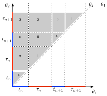
Figure 6: Schematic representation of the different sectors. In the plane $(\theta_{1},\theta_{2})$ we represent the different sectors according to the numbering defined in the text.

Let us illustrate the method on the example of sector 2. For fixed integers $m\geq 1$ and $n\geq m+1$, we have

$$\theta_{1}{\hskip 0.0pt} = {\hskip 0.0pt}\Theta_{1}+B_{1},$$

$$\theta_{2}{\hskip 0.0pt} = {\hskip 0.0pt}\Theta_{2}+B_{2},$$

$$\Theta_{1}{\hskip 0.0pt} = {\hskip 0.0pt}(t_{1}+\cdots+t_{m})+(\tau_{1}+\cdots+\tau_{m-1}),$$

$$\Theta_{2}{\hskip 0.0pt} = {\hskip 0.0pt}(t_{1}+\cdots+t_{n})+(\tau_{1}+\cdots+\tau_{n-1}),$$

$$x(\theta_{1}){\hskip 0.0pt} = {\hskip 0.0pt}t_{1}+\cdots+t_{m},$$

$$x(\theta_{2}){\hskip 0.0pt} = {\hskip 0.0pt}t_{1}+\cdots+t_{n},$$

$$\ell{\hskip 0.0pt} = {\hskip 0.0pt}t_{m+1}+\cdots+t_{n},$$ (16)

with $0<B_{1}<\tau_{m}$ and $0<B_{2}<\tau_{n}$. The contribution of sector 2 with fixed $m$ and $n$ to ${\cal L}(r,s,u)$ therefore reads

$${\cal L}_{2}^{(m,n)}(r,s,u){\hskip 0.0pt} = {\hskip 0.0pt}\biggl{\langle}{\rm e}^{-r\Theta_{1}-s\Theta_{2}-u\ell}$$ (17)

$$\times {\hskip 0.0pt}\int_{0}^{\tau_{m}}\!{\rm e}^{-rB_{1}}\,{\rm d}B_{1}\int_{0}^{\tau_{n}}\!{\rm e}^{-sB_{2}}\,{\rm d}B_{2}\biggr{\rangle}.$$

Hereafter we borrow conventions and notations from Ref. [41]. In particular, $\langle\dots\rangle$ denotes an average over the random process, i.e., over all the move durations $t_{k}$ and rest durations $\tau_{k}$.

The explicit evaluation of (17) involves three steps.

$\bullet$ First, performing the two integrals leads to the expression

$${\cal L}_{2}^{(m,n)}(r,s,u)=\left\langle{\rm e}^{-r\Theta_{1}-s\Theta_{2}-u\ell}\frac{1-{\rm e}^{-r\tau_{m}}}{r}\frac{1-{\rm e}^{-s\tau_{n}}}{s}\right\rangle,$$ (18)

which only involves the $t_{k}$ and $\tau_{k}$.

$\bullet$ Second, averaging independently over all the $t_{k}$ and $\tau_{k}$, we obtain

$${\cal L}_{2}^{(m,n)}(r,s,u){\hskip 0.0pt} = {\hskip 0.0pt}{\widehat{f}}(r+s)^{m}{\widehat{f}}(s+u)^{n-m}{\widehat{g}}(r+s)^{m-1}$$ (19)

$$\times {\hskip 0.0pt}{\widehat{g}}(s)^{n-m-1}\,\frac{{\widehat{g}}(s)-{\widehat{g}}(r+s)}{r}\,\frac{1-{\widehat{g}}(s)}{s}$$

in terms of the Laplace transforms (characteristic functions)

$${\widehat{f}}(s){\hskip 0.0pt} = {\hskip 0.0pt}\langle{\rm e}^{-st}\rangle=\int_{0}^{\infty}f(t)\,{\rm e}^{-st}\,{\rm d}t,$$

$${\widehat{g}}(s){\hskip 0.0pt} = {\hskip 0.0pt}\langle{\rm e}^{-s\tau}\rangle=\int_{0}^{\infty}g(\tau)\,{\rm e}^{-s\tau}\,{\rm d}\tau.$$ (20)

$\bullet$ Third, the entire contribution of sector 2 reads

$${\cal L}_{2}(r,s,u)=\sum_{m=1}^{\infty}\sum_{n=m+1}^{\infty}{\cal L}_{2}^{(m,n)}(r,s,u),$$ (21)

where the sums boil down to geometric sums. This leads to

$${\cal L}_{2}(r,s,u){\hskip 0.0pt} = {\hskip 0.0pt}\frac{{\widehat{f}}(s+u)}{1-{\widehat{f}}(s+u){\widehat{g}}(s)}\,\frac{{\widehat{f}}(r+s)}{1-{\widehat{f}}(r+s){\widehat{g}}(r+s)}$$ (22)

$$\times {\hskip 0.0pt}\frac{{\widehat{g}}(s)-{\widehat{g}}(r+s)}{r}\,\frac{1-{\widehat{g}}(s)}{s}.$$

The contributions of the five other sectors can be evaluated along the same lines. We thus obtain

$${\cal L}_{1}(r,s,u){\hskip 0.0pt} = {\hskip 0.0pt}\frac{{\widehat{f}}(r+s)}{1-{\widehat{f}}(r+s){\widehat{g}}(r+s)}$$

$$\times {\hskip 0.0pt}\frac{r+s{\widehat{g}}(r+s)-(r+s){\widehat{g}}(s)}{rs(r+s)},$$

$${\cal L}_{3}(r,s,u){\hskip 0.0pt} = {\hskip 0.0pt}\frac{1}{1-{\widehat{f}}(s+u){\widehat{g}}(s)}\,\frac{1}{1-{\widehat{f}}(r+s){\widehat{g}}(r+s)}$$

$$\times {\hskip 0.0pt}\frac{{\widehat{f}}(s+u)-{\widehat{f}}(r+s)}{r-u}\,\frac{1-{\widehat{g}}(s)}{s},$$

$${\cal L}_{4}(r,s,u){\hskip 0.0pt} = {\hskip 0.0pt}\frac{1}{1-{\widehat{f}}(r+s){\widehat{g}}(r+s)}$$

$$\times {\hskip 0.0pt}\frac{u-r+(r+s){\widehat{f}}(s+u)-(s+u){\widehat{f}}(r+s)}{(r+s)(u-r)(s+u)},$$

$${\cal L}_{5}(r,s,u){\hskip 0.0pt} = {\hskip 0.0pt}\frac{1}{1-{\widehat{f}}(s+u){\widehat{g}}(s)}\,\frac{{\widehat{f}}(r+s)}{1-{\widehat{f}}(r+s){\widehat{g}}(r+s)}$$

$$\times {\hskip 0.0pt}\frac{{\widehat{g}}(s)-{\widehat{g}}(r+s)}{r}\,\frac{1-{\widehat{f}}(s+u)}{s+u},$$

$${\cal L}_{6}(r,s,u){\hskip 0.0pt} = {\hskip 0.0pt}\frac{{\widehat{g}}(s)}{1-{\widehat{f}}(s+u){\widehat{g}}(s)}\,\frac{1}{1-{\widehat{f}}(r+s){\widehat{g}}(r+s)}$$ (23)

$$\times {\hskip 0.0pt}\frac{{\widehat{f}}(r+s)-{\widehat{f}}(s+u)}{u-r}\,\frac{1-{\widehat{f}}(s+u)}{s+u}.$$

A.3 Steady state

From now on we focus our attention onto the steady state of the process, obtained by letting the first time $\theta_{1}$ go to infinity, keeping the time difference

$$\Delta=\theta_{2}-\theta_{1}$$ (24)

fixed. This steady state is well-defined if the distributions $f(t)$ and $g(\tau)$ decay fast enough for the mean values $\overline{t}$ and $\overline{\tau}$ to be finite. In the opposite situation, where either $\overline{t}$ or $\overline{\tau}$ or even both are divergent, the process never reaches a steady state. It rather exhibits various non-stationary features, usually referred to as aging or weak ergodicity breaking [48]. We assume henceforth that $\overline{t}$ and $\overline{\tau}$ are finite.

The quantity of most interest is the steady-state distribution $P_{\Delta}(\ell)$. Its double Laplace transform

$$L(s,u)=\int_{0}^{\infty}{\rm e}^{-s\Delta}\,{\rm d}\Delta\int_{0}^{\infty}{\rm e}^{-u\ell}\,P_{\Delta}(\ell)\,{\rm d}\ell$$ (25)

is the limit of the product $(r+s){\cal L}(r,s,u)$ as $r\to-s$. We thus obtain

$$L(s,u)=\frac{N(s,u)}{(\overline{t}+\overline{\tau})s^{2}(s+u)^{2}(1-{\widehat{f}}(s+u){\widehat{g}}(s))},$$ (26)

with

$$N(s,u){\hskip 0.0pt} = {\hskip 0.0pt}s(s+u)(s\overline{t}+(s+u)\overline{\tau})(1-{\widehat{f}}(s+u){\widehat{g}}(s))$$ (27)

$$- {\hskip 0.0pt}u^{2}(1-{\widehat{f}}(s+u))(1-{\widehat{g}}(s)).$$

The distribution $P_{\Delta}(\ell)$ has the general form

$$P_{\Delta}(\ell)=C_{0}(\Delta)\,\delta(\ell)+C_{1}(\Delta)\,\delta(\ell-\Delta)+P_{\Delta}^{\rm cont}(\ell),$$ (28)

with two delta functions at the endpoints $\ell=0$ and $\ell=\Delta$, and a non-trivial continuous piece in-between. The delta function at $\ell=0$ corresponds to sector 1 ($\theta_{1}$ and $\theta_{2}$ belong to the same rest duration $\tau_{n}$). The Laplace transform $\widehat{C}_{0}(s)$ of the associated amplitude $C_{0}(\Delta)$ reads

$$\widehat{C}_{0}(s)=\frac{{\widehat{g}}(s)+s\overline{\tau}-1}{(\overline{t}+\overline{\tau})s^{2}},$$ (29)

hence

$$C_{0}(\Delta)=\frac{1}{\overline{t}+\overline{\tau}}\int_{\Delta}^{\infty}(\tau-\Delta)g(\tau)\,{\rm d}\tau.$$ (30)

Similarly, the delta function of $P_{\Delta}(\ell)$ at $\ell=\Delta$ corresponds to sector 4 ($\theta_{1}$ and $\theta_{2}$ belong to the same move duration $t_{n}$). The associated amplitude reads

$$C_{1}(\Delta)=\frac{1}{\overline{t}+\overline{\tau}}\int_{\Delta}^{\infty}(t-\Delta)f(t)\,{\rm d}t.$$ (31)

As $\Delta$ increases from 0 to infinity, the above amplitudes decrease monotonically from $C_{0}(0)=\overline{\tau}/(\overline{t}+\overline{\tau})$ and $C_{1}(0)=\overline{t}/(\overline{t}+\overline{\tau})$ to zero, whereas the weight of the continuous part $P_{\Delta}^{\rm cont}(\ell)$ increases from zero to one.

The mean value of $\ell$ has the remarkably simple expression

$$\langle\ell\rangle_{\Delta}=\frac{\overline{t}}{\overline{t}+\overline{\tau}}\,\Delta.$$ (32)

The second moment of $\ell$ reads in Laplace space

$$\int_{0}^{\infty}{\rm e}^{-s\Delta}\langle\ell^{2}\rangle_{\Delta}\,{\rm d}\Delta{\hskip 0.0pt} = {\hskip 0.0pt}\frac{2\overline{t}}{(\overline{t}+\overline{\tau})s^{3}}$$ (33)

$$- {\hskip 0.0pt}\frac{2(1-{\widehat{f}}(s))(1-{\widehat{g}}(s))}{(\overline{t}+\overline{\tau})s^{4}(1-{\widehat{f}}(s){\widehat{g}}(s))}.$$

This formula can be inverted in the regime where $\Delta$ is much larger than $\overline{t}$ and $\overline{\tau}$, yielding

$$\langle\ell^{2}\rangle_{\Delta}-\langle\ell\rangle_{\Delta}^{2}\approx\frac{(\overline{\tau^{2}}-\overline{\tau}^{2})\overline{t}^{2}+(\overline{t^{2}}-\overline{t}^{2})\overline{\tau}^{2}}{(\overline{t}+\overline{\tau})^{3}}\,\Delta+K.$$ (34)

The linear growth of the variance of $\ell$ with $\Delta$ testifies that the continuous part $P_{\Delta}^{\rm cont}(\ell)$ satisfies an approximate central limit theorem at large $\Delta$, where the measured displacement $\ell$ is the sum of a typically large number of elementary moves. The constant $K$, corresponding to the first correction to this limit, is given by a combination of moments of $t$ and $\tau$, which can be either positive or negative.

Another quantity which is used in the main text is the fraction $P_{\rm good}(\Delta)$ of the moves which are correctly sampled. These events correspond to the observation times $\theta_{1}$ and $\theta_{2}$ belonging to two consecutive rests surrounding the move under consideration, i.e., to sector 2 with $n=m+1$. It is also useful to introduce the normalised fraction of correctly sampled moves,

$$F_{\rm good}(\Delta)=\frac{P_{\rm good}(\Delta)}{1-C_{0}(\Delta)},$$ (35)

where the denominator is nothing but the probability of measuring a non-zero displacement.

In the steady-state of the process, we obtain in Laplace space

$$\widehat{P}_{\rm good}(s)=\frac{{\widehat{f}}(s)(1-{\widehat{g}}(s))^{2}}{(\overline{t}+\overline{\tau})s^{2}},$$ (36)

whereas the Laplace transform of $C_{0}(\Delta)$ is given by (29).

A.4 Exponential distributions

When the distributions of the move and rest durations are exponential, with respective parameters $a=1/\overline{t}$ and $b=1/\overline{\tau}$, i.e., $f(t)=a\,{\rm e}^{-at}$, $g(\tau)=b\,{\rm e}^{-b\tau}$, ${\widehat{f}}(s)=a/(s+a)$, ${\widehat{g}}(s)=b/(s+b)$, the above expressions simplify drastically, and so many observables can be evaluated in closed form.

Eqs. (26), (27) read

$$L(s,u)=\frac{(a+b)^{2}+(a+b)s+au}{(a+b)(s^{2}+(a+b+u)s+bu)}.$$ (37)

We thus recover (32), i.e.,

$$\langle\ell\rangle_{\Delta}=\frac{b}{a+b}\,\Delta,$$ (38)

as well as the following expression

$$\langle\ell^{2}\rangle_{\Delta}=\langle\ell\rangle_{\Delta}^{2}+\frac{2ab}{(a+b)^{3}}\,\Delta+\frac{2ab}{(a+b)^{4}}\left({\rm e}^{-(a+b)\Delta}-1\right)$$ (39)

for the second moment of the measured displacement. In this example, the constant $K=-2ab/(a+b)^{4}$ is negative. Higher moments can be evaluated as well.

With the notations of the main text, i.e., in terms of $\overline{\tau},\overline{t},\ell^{\ast},v,\overline{\Delta}$, the first two moments read

$$\langle\ell^{\ast}\rangle=\frac{v\overline{\Delta}}{1+\overline{\tau}/\overline{t}}$$ (40)

and

$$\langle\ell^{\ast 2}\rangle =\frac{v^{2}\overline{\Delta}^{2}}{(1+\overline{\tau}/\overline{t})^{2}}+\frac{2v^{2}\overline{\tau}^{2}\overline{\Delta}}{\overline{t}(1+\overline{\tau}/\overline{t})^{3}}$$

$$+\frac{2v^{2}\overline{\tau}^{3}}{\overline{t}(1+\overline{\tau}/\overline{t})^{4}}\left(\exp\left({-\frac{(\overline{t}+\overline{\tau})\overline{\Delta}}{\overline{t}\overline{\tau}}}\right)-1\right).$$ (41)

The full distribution $P_{\Delta}(\ell)$ can also be obtained in closed form. In a first step, performing the inverse transform of the expression (37) from $s$ to $\Delta$, we obtain an expression for the Laplace transform

$$L_{\Delta}(u)=\int_{0}^{\infty}{\rm e}^{-u\ell}P_{\Delta}(\ell)\,{\rm d}\ell,$$ (42)

namely

$$L_{\Delta}(u){\hskip 0.0pt} = {\hskip 0.0pt}{\rm e}^{-(a+b+u)\Delta/2}$$ (43)

$$\times {\hskip 0.0pt}\!\left(\!\cosh R+\frac{(a+b)^{2}+(a-b)u}{2(a+b)}\frac{\sinh R}{R}\Delta\!\right)\!,$$

with

$$R=\frac{\Delta}{2}\,\sqrt{(a-b+u)^{2}+4ab}.$$ (44)

In a second step, the expression (43) can be inverse transformed from $u$ to $\ell$, yielding an end result of the expected general form (28), with

$$C_{0}(\Delta)=\frac{a}{a+b}\,{\rm e}^{-b\Delta},\quad C_{1}(\Delta)=\frac{b}{a+b}\,{\rm e}^{-a\Delta}$$ (45)

and

$$P_{\Delta}^{\rm cont}(\ell){\hskip 0.0pt} = {\hskip 0.0pt}\frac{2ab}{a+b}\,{\rm e}^{-a\ell-b(\Delta-\ell)}$$ (46)

$$\times {\hskip 0.0pt}\left(I_{0}(x)+(a(\Delta-\ell)+b\ell)\frac{I_{1}(x)}{x}\right),$$

with

$$x=2\sqrt{ab\ell(\Delta-\ell)},$$ (47)

and where $I_{0}$ and $I_{1}$ are modified Bessel functions.

The expression (36) reads

$$\widehat{P}_{\rm good}(s)=\frac{a^{2}b}{(a+b)(a+s)(b+s)^{2}}.$$ (48)

We have therefore

$$P_{\rm good}(\Delta){\hskip 0.0pt} = {\hskip 0.0pt}\frac{a^{2}b}{(a+b)(a-b)^{2}}$$ (49)

$$\times {\hskip 0.0pt}\left({\rm e}^{-a\Delta}+((a-b)\Delta-1){\rm e}^{-b\Delta}\right)$$

and

$$F_{\rm good}(\Delta)=\frac{a^{2}b}{(a-b)^{2}}\,\frac{{\rm e}^{-a\Delta}+((a-b)\Delta-1){\rm e}^{-b\Delta}}{a+b-a\,{\rm e}^{-b\Delta}}.$$ (50)

The normalised fraction $F_{\rm good}(\Delta)$ of correctly sampled moves starts growing as $(a\Delta)^{2}/2$ at small $\Delta$, whereas it falls off exponentially at large $\Delta$. It therefore reaches a non-trivial maximum $\hat{F}_{\rm good}$ for an optimal value $\hat{\Delta}$ of $\Delta$ (see Fig. S2). In the limit $b/a\to 0$, the maximal value $\hat{F}_{\rm good}$ reaches unity. It is attained for

$$\hat{\Delta}\approx\frac{2}{\sqrt{ab}}.$$ (51)

It however drops from this perfect value very rapidly, with a square-root singularity of the form

$$\hat{F}_{\rm good}\approx 1-2\sqrt{\frac{b}{a}}.$$ (52)

For $a=b$, the expression (50) simplifies to

$$F_{\rm good}(\Delta)=\frac{(a\Delta)^{2}}{2(2{\rm e}^{a\Delta}-1)}.$$ (53)

The maximal value is already as small as $\hat{F}_{\rm good}\approx 0.14602$. It is reached for $\hat{\Delta}\approx 1.84141/a$.

Supplementary Information

Appendix S1 Supplementary Figures

Mobility represented	$\overline{t}$ (h)	$\overline{\tau}$ (h)	$P(\tau)$	Sampling	Type of result	$F_{good}$	Notes
Italian cars	0.30	2.49	Exponential	Periodic	Analytical	51%	$\overline{\Delta}=1.7$h
			Stretched exponential	Periodic	Numerical	39%	$\overline{\Delta}=1.3$h
			Exponential	Power law	Numerical	27%	–
			Stretched exponential	Power law	Numerical	23%	–
USA CDR data	(0.30)	0.55	Exponential	Periodic	Analytical	24%	$\overline{\Delta}=0.8$h
			Truncated power law	Periodic	Numerical	15%	$\overline{\Delta}=0.5$h
			Truncated power law	Power law	Numerical	6%	–
Chinese Geolife Traj.	0.33	0.80	Exponential	Periodic	Analytical	27%	$\overline{\Delta}=1.0$h
			Empirical	Periodic	Numerical	18%	$\overline{\Delta}=1.0$h
			Empirical	Empirical ($p=0$)	Numerical	11%	–
			Empirical	Empirical ($p=1$)	Numerical	16%	–

Table 1: Results’ summary.

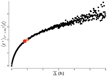
Figure S2: Constant sampling on GPS data. We present results obtained by sampling the GeoLife GPS data with a constant sampling interval $\Delta$. We plot the average sampled move displacement (computed in 2 dimensions) ($\langle\ell^{\ast}\rangle_{\ell^{\ast}>0}$ normalized by the real average move length $\langle\ell\rangle$ as a function of the length of the sampling interval $\overline{\Delta}$. The ideal case $\langle\ell^{\ast}\rangle_{\ell^{\ast}>0}=\langle\ell\rangle$ (Eq. (9)) is reached for $\overline{\Delta}=15$ min, while for a short-tailed rest time it is expected to be $\overline{\Delta}=52$ min (red circle). The fact that the sampling time optimizing $F_{\rm good}$ (orange triangle) corresponds to $\langle\ell^{\ast}\rangle_{\ell^{\ast}>0}/\langle\ell\rangle\approx 2$ implies that optimal sampling frequencies would represent, in this case, an under-sampling of the trajectory where moves are more frequently joined together than cut by sampling times.

Appendix S2 Numerical Analysis

S2.1 Random sampling and long-tailed pause distributions

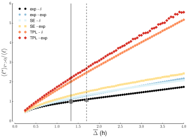
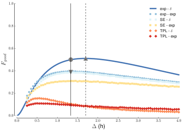
Figure S4: Effect of sampling (periodic and Poisson process) with different rest distribution. Similar to what we depicted in Fig. 3 (represented here as black circles in the left panel and as a blue line in the right panel). In all scenarios studied, we fix $\overline{t}=0.30$ h and consider different alternative forms for $P(\tau)$ (exponential (exp–) or Stretched Exponential (SE–) or Truncated Power Law (TPL–)). We use either constant (–$\delta$) or exponentially distributed (–exp) sampling times. The grey circle represents the value associated with $\mathring{\Delta}$ and the grey triangle that of $\hat{\Delta}$ for the (exp – $\delta$) scenario. (Left) We compare the average value $\langle\ell^{\ast}\rangle_{\ell^{\ast}>0}$ with $\langle\ell\rangle=\overline{\ell}=v\overline{t}$. All definitions of the optimal sampling time which are different from $\mathring{\Delta}$ (defined by imposing the identity between $\langle\ell^{\ast}\rangle$ and $\overline{\ell}$) are necessarily associated to values smaller than $\mathring{\Delta}$ for long-tailed rest distributions. For the SE case, a sampling time of $\approx 1$h correctly estimates the average. If rests are distributed as a TPL, the large fraction of short rests leads to the concatenation of subsequent trips, even with this relatively short sampling time. This result illustrates a first incongruence in the work by Song et al. [4], where individual moves and rests are reconstructed with a sampling rate of 1 h, identifying a rest distribution (the TPL studied here) for which we predict that only half of the movements would be captured (because $\langle\ell^{\ast}\rangle/\overline{\ell}\approx 2$ and consequently $n^{\ast}/n\approx 1/2$). (Right) In all scenarios the fraction $F_{\rm good}$ of correctly sampled trips is lower than the value (51%) given by Eq. (14) and studied extensively in this paper. In particular, trajectories with long rest times (SE– and TPL–) yield worse results than the peaked case (exp–). At the same time, using exponentially distributed sampling times (–exp) systematically yields worse results than constant sampling (–$\delta$). The optimal value $\hat{\Delta}$ (up triangle and dashed line) over-estimates the position of the peak for long-tailed rests. A possible realistic scenario for human mobility is represented by a down triangle, where trajectories with SE rest distribution reach a maximum $F_{\rm good}$ of 39% when sampled with a constant $\overline{\Delta}=\check{\Delta}=1.33$ h (80 min). If the pause distribution is TPL, $F_{\rm good}$ barely reaches the $15\%$ mark, illustrating a second incongruence in the work by Song et al. [4].

As stated in the main text, real sampling problems can be more complex than the idealized case defined by Eqs. (1), (2) and (3). In particular: (i) the rest time distribution can be broad; (ii) sampling times can be random variables; (iii) speed can be a random variable (Travel durations have been seen to have a short-tailed distribution). We start by studying the effects of points (i) and (ii), while we discuss point (iii) in the following section.

Available data on rest durations suggest that their distribution is long-tailed. Different fits have been proposed for the latter distribution. Here we consider a Truncated Power Law (TPL), used for interpreting mobile phone data [4], and a Stretched Exponential (SE), used for interpreting private vehicles’ parking times [7]. As for the sampling time, we can introduce randomness with an exponential distribution of inter-event times (Poisson process). Alternatively, if we want to represent the sampling process associated to communication, we use a power-law distribution with exponent $-1$ [33,3]. Since this distribution is not integrable, it is necessarily defined on an interval between some $\Delta_{\rm min}$ and $\Delta_{\rm max}$.

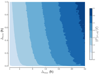
(a)	(b)
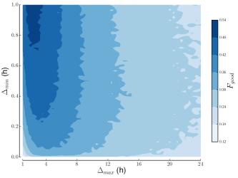
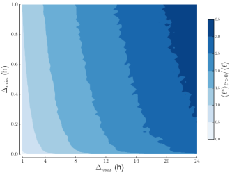
(c)	(d)
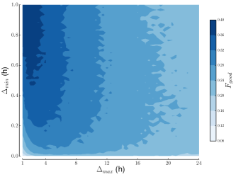
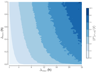
(e)	(f)

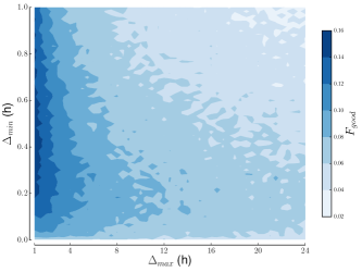
Figure S5: Effect of sampling with power-law inter-event times and different rest distributions. Using sampling times distributed similarly to communication patterns, samplings get very bad for Exponential (a, b), Stretched Exponential (c, d) or Truncated Power Law (e, f) rest distributions. The quality of the sampling depends on how we choose the minimal $\Delta_{\rm min}$ and maximal $\Delta_{\rm max}$ inter-event times. The left panels show the error in the estimate of the average $\langle\ell\rangle$. The right panels represent the fraction $F_{\rm good}$ of correctly sampled moves. With a very conservative choice of $\Delta_{\rm min}=5$ min and $\Delta_{\rm max}=12$ h, the value $F_{\rm good}$ for the exponential rest distribution drops from $\approx 51\%$ to $\approx 27\%$. For long-tailed rests we are limited to a maximal $F_{\rm good}\approx 23\%$ (panel (d), Stretched Exponential) when sampling human trajectories with mobile phones. The value drops below $6\%$ in the same conditions for the Truncated Power Law (panel (f)).

In Figs. S4 and S5, we combine different rest distributions and sampling time distributions. We see that, in all the possible scenarios, $F_{\rm good}$ is below the best value $\hat{F}_{\rm good}=51\%$. In Fig. S4 (right) we show the fraction $F_{\rm good}$ for exponential (exp), TPL or SE rest time distributions and with sampling times $\Delta$ distributed as a delta function ($P(\Delta)=\delta(\Delta-\overline{\Delta})$) or an exponential distribution ($P(\Delta)=(1/\overline{\Delta})\exp(-\Delta/\overline{\Delta})$), associated to a Poisson process where a sampling can happen at each moment with uniform rate. The solid blue line, together with the gray circle and the up triangle markers, represent the same information as displayed in Fig. 2 (d). All the other curves for $F_{\rm good}(\overline{\Delta})$ are bell-shaped, their maxima have heights $<51\%$, and these maxima are reached for a $\overline{\Delta}$ close to the expected $\hat{\Delta}$. Therefore, all variations introduced here only yield worse samplings. With a down triangle we show that, when the rest times are distributed as a Stretched Exponential, as suggested by car mobility data, the optimal sampling time would be $\check{\Delta}\approx 1.33$ h, but with only 39% of trips correctly sampled. If rest times have instead a TPL distribution, as estimated by mobile phone data [4], the sampling is very poor, with $F_{\rm good}<15\%$.

Panels (b) (d) and (f) of Fig. S5 correspond to a power-law sampling, where the final result is of course dependent upon $\Delta_{\rm min}$ and $\Delta_{\rm max}$. $F_{\rm good}$ never goes over the optimal value found for constant sampling, which is naturally reached when $\Delta_{\rm min}$ and $\Delta_{\rm max}$ get close to $\hat{\Delta}$. However, since in an individual behavior we can easily have a whole day without communication, the values of $F_{\rm good}$ we expect would be more of the order of the values reached on the right half of each contour graph. We consider as reference values (here as for our analysis of the GeoLife trajectory) $\Delta_{\rm min}=5$ min and $\Delta_{\rm max}=12$ h. This very conservative choice yields $F_{\rm good}=27\%$ for the exponential rest distribution.

For both constant and random sampling times, the SE distribution yields values of $F_{\rm good}$ better than the TPL. This is expected, since larger values of $\overline{\tau}$ are associated to a better sampling (see Fig. 4 (top)), and confirms our choice of the characteristic times for vehicular mobility as the best-case scenario for our study. We therefore identify as ‘optimistic’ values for $F_{\rm good}$ for a realistic distribution of rests (the Stretched Exponential) the value $39\%$ for constant sampling and $23\%$ for power-law sampling. This last value is, again, computed with $\Delta_{\rm min}=5$ min and $\Delta_{\rm max}=12$ h.

In conclusion of this section, we cannot help but remark the incongruence between the rest time distribution identified from CDR data (the TPL studied here) and the sampling time of $1$ h used to identify mobility patterns. For such a rest time distribution we predict $\langle\ell^{\ast}\rangle/\overline{\ell}\approx 2$ for a sampling time of $1$ h. This ratio suggests that the trajectory is largely under-sampled, with only about half the trips correctly identified. Since rests would also be consequently under-counted, and thus over-estimated in duration, the rest time distribution estimated cannot be correct either.

S2.2 Effect of velocity and spatial embedding

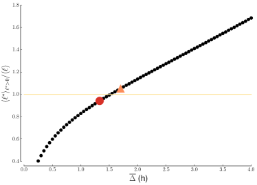
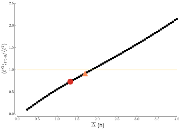
Figure S6: Moments of $P(\ell^{\ast})$ with speed variability in the peaked scenario. (Left) First moment. (Right) Second moment. We introduce variability in the speed distribution $P(v)$, using a random acceleration model [7]. This introduces only minor changes in estimating the moments. The red circle indicates the result using the sampling time $\mathring{\Delta}$ that matches the mean values ($\langle\ell^{\ast}\rangle=\overline{\ell}$). The orange triangle shows the values associated to $\hat{\Delta}$, the sampling time maximizing $F_{\rm good}$. The first sampling time $\mathring{\Delta}$ yields a slightly under-estimated first and second moment, with a deviation of $5\%$ and $20\%$ respectively, with respect to the moments of the displacement distribution in the simulated trajectories (yellow solid line).

We have seen that the optimal sampling times defined in the main text do not depend upon the nature of $P(v)$, nor on the dimensionality of space (and thus of the vector speed $v$). Even when introducing these two factors, the fraction of moves that have been correctly identified remains unchanged. Nevertheless, the shape of the distribution $P(\ell^{\ast})$ of sampled distances necessarily depends on speed and spatial embedding. We illustrate this by using, on top of the conditions set by Eqs. (1), (2) and (3), a random acceleration mobility model that induces a correlation between travel time and speed consistent with real data at a national level [7]. The results of Fig. S6 are to be compared with those of Fig. 3 (top) in the main text. In this case, the sampling time $\hat{\Delta}$ that is expected to match the first moment for constant speed under-estimates the average displacement by about $5\%$.

In Fig. S6 (left) we show the effect of sampling trajectories with speed variability. We observe that, when the sampling time distribution is broad, we have the larger deviations from the original distribution. This same phenomenon can also be seen in Fig. S4 (left), where we show that the mean value $\langle\ell^{\ast}\rangle$ is significantly larger when the rest distribution is broad. The issue comes by the fact that with broad distributions we have several instances where the sampling time is large with respect to the average rest, and therefore more jumps are joined together. When this happens, the dimensionality and the nature of the turning angle distribution becomes important. Fig. S7 would differ significantly by introducing this further element. Indeed, at low frequencies one would have to integrate over many re-orientations [26]. These re-orientations are neglected in our one-dimensional picture, that as a consequence over-estimates this sum. A possible multi-dimensional model could be the worm-like chain. On top of this, since the human tendency of returning home limits the space explored [3], the size of these summed displacements could be further reduced.

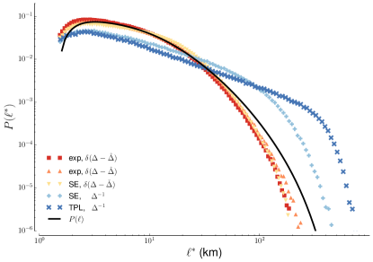
Figure S7: Sampling accelerated trajectories. Using a random acceleration model [7], we study how the displacement distribution changes with the sampling. The result depends upon the rest time distribution (exponential (exp), stretched exponential (SE) and truncated power law (TPL)) and on the sampling time distribution (peaked $\delta(\Delta-\bar{\Delta})$ or with a long tail (PL)). The optimal sampling times ($\hat{\Delta}$ and $\mathring{\Delta}$, defined in the main text and $\check{\Delta}$ defined in the preceding section) give reasonably good results, while long-tailed sampling creates sizeable deviations in the displacement distribution.

S2.3 Correlations between calls and rests in empirical sampling

In the main text we study how the statistical properties of GPS trajectories of individuals are affected when we sample them with an inter-call distribution extracted from mobile phone data (CDR). It can however be objected that the times at which calls are made are correlated to the rests. Hence the fraction of correctly sampled trips might be higher than the one we obtain without correlations.

Moreover, more refined method of trajectory extraction are based on the idea of identifying stays (where the user is performing an activity) and pass-by’s (locations where the call is made during a travel) [40]. Normally, one needs at least two calls in the same stay to identify it correctly as an activity. The goal of this method consists in filtering out calls made during rests. An ideal algorithm that perfectly identifies calls done during moves would then be equivalent to a perfect correlation between rests and calls.

For these reasons, we study the effect of correlations on the fraction of correctly sampled trajectories. We introduce a parameter $p$ to quantify the extent of correlations between calls and rests. Any call that is performed during a move is excluded with probability $1-p$. When $p=0$ calls and rests are decorrelated, while they are perfectly correlated (all calls necessarily happen when at rest) when $p=1$.

The results are presented on Fig. S8: when $p=0$ we find the same value $F_{\rm good}=11\%$ as presented in the main text. When $p=1$ we find $F_{\rm good}=16\%$, which is indeed better than without correlations, yet not large enough to invalidate our conclusions, nor to support the current ‘stay point identification’ method as sufficient for reconstructing mobility patterns.

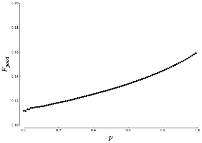
Figure S8: Effect of correlations on the fraction of correctly sampled trajectories. We quantify the effect of correlations between calls and rests on the fraction of rightly sampled trips $F_{\rm good}$. When $p=0$ calls and rests are uncorrelated and we find $F_{\rm good}=11\%$, as shown in the main text. When $p=1$ calls only happen during rests and we find $F_{\rm good}=16\%$. Our conclusions therefore hold disregarding of whether there are correlations between calls and movements, or if this correlation is induced by filtering out calls done during moves.

References

- (1) A. Vespignani, Modelling dynamical processes in complex socio-technical systems, Nat Phys 8, 32–39 (2012).
- (2) Y. Zheng, Trajectory data mining: An overview, ACM Transactions on Intelligent Systems and Technology 6, 29–41 (2015).
- (3) M. C. González, C. A.Hidalgo, and A.-L.Barabási, Understanding individual human mobility patterns, Nature 453(7196), 779–782 (2008).
- (4) C. Song C, T. Koren, P. Wang, and A.-L. Barabási, Modelling the scaling properties of human mobility, Nat Phys 6(10), 818–823 (2010).
- (5) D. A. Raichlen, B. M. Wood, A. D. Gordon, A. Z. Mabulla, F. W. Marlowe, and H. Pontzer, Evidence of Lévy walk foraging patterns in human hunter-gatherers, Proc Natl Acad Sci USA 111, 728–733 (2014).
- (6) R. Gallotti, A. Bazzani, and S. Rambaldi, Understanding the variability of daily travel-time expenditures using GPS trajectory data, EPJ Data Science 4, 18 (2015).
- (7) R. Gallotti, A. Bazzani, S. Rambaldi, M. Barthélemy, A stochastic model of randomly accelerated walkers for human mobility, Nature Communications 7, 12600 (2016).
- (8) D. Balcan, V. Colizza,, B. Gon alves,H. Hu, J. J. Ramasco, and A. Vespignani, Multiscale mobility networks and the spatial spreading of infectious diseases, Proc Natl Acad Sci USA 106, 21484–21489 (2009).
- (9) G. M. Viswanathan ,M. G. E. Da Luz, E. P Raposo, and H. E Stanley, The physics of foraging: an introduction to random searches and biological encounters, (Cambridge University Press 2011).
- (10) A. Reynolds, Liberating Lévy walk research from the shackles of optimal foraging, Phys Life Rev 14, 59–83 (2015).
- (11) D. Brockmann, L. Hufnagel, and T. Geisel, The scaling laws of human travel, Nature 439, 462–465 (2006).
- (12) S. Phithakkitnukoon, M. I. Wolf, D. Offenhuber, D. Lee, A. Biderman, and C. Ratti, Tracking trash, IEEE Pervas Comput 12, 38–48 (2013).
- (13) F. Cagnacci, L. Boitani, R. A. Powell, and M. S. Boyce, Animal ecology meets GPS-based radiotelemetry: a perfect storm of opportunities and challenges, Philos T R Soc B 365, 2157–2162 (2010).
- (14) O. Sagarra, M. Szell, P. Santi, A. Díaz-Guilera, and C. Ratti, Supersampling and network reconstruction of urban mobility, PLoS ONE 10(8), e0134508 (2015).
- (15) N. E. Williams, T. A. Thomas, M. Dunbar, N. Eagle, and A. Dobra, Measures of human mobility using mobile phone records enhanced with GIS data, PLoS ONE 10(7), e0133630 (2015).
- (16) S. Çolak, L. P. Alexander, B. G. Alvim, S. R. Mehndiratta, M. C. González, Analyzing cell phone location data for urban travel, Transp Res Record 2526, 126–135 (2016).
- (17) P. Turchin, Quantitative analysis of movement: measuring and modeling population redistribution in animals and plants, (Sinauer Associates, Sunderland 1998).
- (18) E. A. Codling, M. J Plank, and S. Benhamou, Random walk models in biology, J R Soc Interface 5, 813–834 (2008).
- (19) M. Hebblewhite and D. T. Haydon, Distinguishing technology from biology: a critical review of the use of GPS telemetry data in ecology, Philos T R Soc B 365, 2303–2312 (2010).
- (20) P. Laube and R. S. Purves, How fast is a cow? Cross–Scale Analysis of Movement Data, Transactions in GIS 15, 401–418 (2011).
- (21) D. D. Salvucci and J. H. Goldberg, Identifying fixations and saccades in eye-tracking protocols, Proceedings of the 2000 symposium on Eye tracking research & applications 71–78 (2000).
- (22) R. Kitamura, S. Fujii, E. I. Pas, Time-use data, analysis and modeling: toward the next generation of transportation planning methodologies, Transp Policy 4, 225–235 (1997).
- (23) J. M. Fryxell, M. Hazell, L. Börger, B. D. Dalziel, D. T. Haydon, J. M. Morales, T. McIntosh, and R. C. Rosatte, Multiple movement modes by large herbivores at multiple spatiotemporal scales, Proc Natl Acad Sci USA 105, 19114–19119 (2008).
- (24) A. M. Edwards, Overturning conclusions of Lévy flight movement patterns by fishing boats and foraging animals, Ecology 92, 1247–1257 (2011).
- (25) E. A. Codling and N.A. Hill, Sampling rate effects on measurements of correlated and biased random walks, J Theor Biology 233, 573–588 (2005).
- (26) G. Rosser, A. G. Fletcher, P. K. Maini, and R. E. Baker, The effect of sampling rate on observed statistics in a correlated random walk, J R Soc Interface 10, 20130273 (2013).
- (27) W. J. Reed and B. D. Hughes, From gene families and genera to incomes and internet file sizes: why power laws are so common in nature, Phys Rev E 66, 067103 (2002).
- (28) G. Mosetti, G. Jug and E. Scalas, Power laws from randomly sampled continuous-time random walks, Physica A 375, 233–238 (2007).
- (29) M. J. Plank and E. A. Codling, Sampling rate and misidentification of Lévy and non-Lévy movement paths, Ecology 90(12), 3546–3553 (2009).
- (30) E. A. Codling and M. J. Plank, Turn designation, sampling rate and the misidentification of power laws in movement path data using maximum likelihood estimates, Theor Ecol 4, 397–406 (2011).
- (31) V. D. Blondel, A. Decuyper, and G. Krings, A survey of results on mobile phone datasets analysis, EPJ Data Science 4, 10 (2015).
- (32) B. Hawelka, I. Sitko, E. Beinat, S. Sobolevsky, P. Kazakopoulos, and C. Ratti, Geo-located Twitter as proxy for global mobility patterns, Cartogr Geogr Inform 41(3), 260–271 (2014).
- (33) A.-L. Barabási, The origin of bursts and heavy tails in human dynamics, Nature 435(7039), 207–211 (2005).
- (34) D. R. Bild, Y. Liu, R. P. Dick, Z. M. Mao, and D. S. Wallach, Aggregate characterization of user behaviour in Twitter and analysis of the retweet graph, ACM Transactions on Internet Technology 15(1), 4 (2015).
- (35) C. Song, Z. Qu, N. Blumm, and A.-L. Barabási, Limits of predictability in human mobility, Science 327(5968), 1018–1021 (2010).
- (36) L. Pappalardo, F. Simini, S. Rinzivillo, D. Pedreschi, F. Giannotti, and A. L. Barabási, Returners and explorers dichotomy in human mobility, Nat Commun 6, 8166 (2015).
- (37) H. Barbosa, F. B. de Lima-Neto, A. Evsukoff, and R. Menezes, The effect of recency to human mobility, EPJ Data Science 4, 21 (2015).
- (38) L. Pappalardo, S. Rinzivillo, and F. Simini, Human mobility modelling: exploration and preferential return meet the gravity model, Procedia Computer Science 83, 934 – 939 (2016).
- (39) J. P. Bagrow and Y.-R. Lin, Mesoscopic structure and social aspects of human mobility, PLoS ONE 7, e37676 (2012).
- (40) S. Jiang, G. A. Fiore, Y. Yang, J. Ferreira Jr, E. Frazzoli, and M. C. González, A Review of Urban Computing for Mobile Phone Traces: Current Methods, Challenges and Opportunities, Proceedings of the 2nd ACM SIGKDD International Workshop on Urban Computing, UrbComp’13, 1–9 (2013).
- (41) C. Godrèche and J. M. Luck, Statistics of the occupation time of renewal processes, J Stat Phys 104, 489–524 (2001).
- (42) A. Reynolds, How many animals really do the Lévy Walk? Comment, Ecology 89, 2347–2351 (2008).
- (43) S. Benhamou, How many animals really do the Lévy Walk? Reply, Ecology 89, 2351–2352 (2008).
- (44) S. Hoteit, S. Secci, S. Sobolevsky, C. Ratti, and G. Pujolle, Estimating human trajectories and hotspots through mobile phone data, Computer Networks 64, 296–307 (2014).
- (45) W. Feller, An Introduction to Probability Theory and its Applications (Wiley, New York 1968).
- (46) D. R. Cox, Renewal theory (Methuen, London 1962).
- (47) D. R. Cox DR, and H. D. Miller, The Theory of Stochastic Processes (Chapman & Hall, London 1965).
- (48) R. Metzler, J. H. Jeon, A. G. Cherstvy, and E. Barkai, Anomalous diffusion models and their properties: non-stationarity, non-ergodicity, and ageing at the centenary of single particle tracking, Phys Chem Chem Phys 16, 24128–24164 (2014).
- (49) F. Giannotti, M. Nanni, F. Pinelli, and D. Pedreschi, Trajectory pattern mining, 13th ACM SIGKDD international conference, 330–339 (2007).
- (50) H. Wang, F. Calabrese, G. Di Lorenzo, and C. Ratti, Transportation mode inference from anonymized and aggregated mobile phone call detail records, 13th International IEEE Conference on Intelligent Transportation Systems, 318–323 (2010).
- (51) P. Ranacher, R. Brunauer, W. Trutschnig, S. Van der Spek, and S. Reich, Why GPS makes distances bigger than they are, Int J Geogr Inf Sci 30(2), 316–333 (2016).
- (52) R. Gallotti, A. Bazzani, and S. Rambaldi, Towards a statistical physics of human mobility, Int J Mod Phys C 23, 1250061 (2012).
- (53) A. Proekt, J. R. Banavar, A. Maritan, and D. W. Pfaff, Scale invariance in the dynamics of spontaneous behavior, Proc Natl Acad Sci USA 109(26), 10564–10569 (2012).
- (54) Y. Zheng, X. Xie, and W.-Y. Ma, GeoLife: A Collaborative Social Networking Service among User, location and trajectory, IEEE Data Engineering Bulletin 33(2), 32–40 (2010).
- (55) K. Zhao, M. Musolesi, P. Hui, W. Rao, and S. Tarkoma, Explaining the power-law distribution of human mobility through transportation modality decomposition, Sci Rep 5, 9136 (2015).
- (56) Y. A. de Montjoye, Z. Smoreda, R. Trinquart, C. Ziemlicki, and V. D. Blondel, D4D-Senegal: the second mobile phone data for development challenge, preprint arXiv:1407.4885 (2014).
- (57) R. Gallotti, A. Bazzani, M. Degli Esposti, and S. Rambaldi, Entropic measures of individual mobility patterns, J Stat Mech 2013, P10022 (2013).
- (58) A. Cuttone, S. Lehmann, and M. C. González, Understanding Predictability and Exploration in Human Mobility, preprint arXiv:1608.01939 (2016).