Semiclassical Propagation: Hilbert Space vs. Wigner Representation

Abstract

A unified viewpoint on the van Vleck and Herman-Kluk propagators in Hilbert space and their recently developed counterparts in Wigner representation is presented. It is shown that the numerical protocol for the Herman-Kluk propagator, which contains the van Vleck one as a particular case, coincides in both representations. The flexibility of the Wigner version in choosing the Gaussians’ width for the underlying coherent states, being not bound to minimal uncertainty, is investigated numerically on prototypical potentials. Exploiting this flexibility provides neither qualitative nor quantitative improvements. Thus, the well-established Herman-Kluk propagator in Hilbert space remains the best choice to date given the large number of semiclassical developments and applications based on it.

Introduction.

The idea to utilize simple and robust tools of classical mechanics for describing quantum-mechanical effects is extremely tempting. In this context, semiclassical techniques are attracting a never-fading interest, since van Vleck (vV) proposed a semiclassical propagator which is exclusively based on classical trajectories. Van Vleck (1928); Littlejohn (1992) However, the original semiclassical approaches suffer from conceptual intrinsic problems that mostly originate from the fact that classical mechanics operates in phase space (position and momentum), whereas a standard formulation of quantum mechanics is in Hilbert space (based on position or momentum wavefunctions). This makes a connection between the two theories not straightforward. In particular, employing the original vV formulation for numerical simulations is hindered due to the infamous root-search problem related to two-sided boundary conditions in position-space propagation. This gave rise to initial-value representations (IVRs) that are exploiting initial position-momentum pairs instead of initial and final positions (or momenta), see Refs. Miller, 2001; Thoss and Wang, 2004; Kay, 2005 for reviews. Further attempt to formulate the theory in terms of phase space objects was based on expanding the evolution operator in the coherent states’ basis leading to the Herman-Kluk (HK) propagator, Herman and Kluk (1984); Kluk, Herman, and Davis (1986) which can be derived by different means Kay (1994a, 2006); Grossmann and Xavier (1998); Miller (2002a, b); Child and Shalashilin (2003); Deshpande and Ezra (2006) and viewed as a frozen-Gaussian Heller (1981) IVR approximation.

One can show that in their Hilbert space formulations the vV propagator is a (non-optimal) limiting case of the HK one if the width of the underlying Gaussians tends to zero either in positions or in momenta, referred to as position vV or momentum vV, respectively. Miller (2001) Interestingly, the HK propagator can be also derived from the vV propagator by either performing a stationary phase approximation Grossmann (2013) or by applying a modified Filinov transform. Miller (2002a) These relations underline the principal semiclassical equivalence of the two propagators, although there have been misunderstandings about the HK propagator being inferior to the vV propagator, see Ref. Kay, 2005 for a detailed discussion.

A historically different way of putting classical and quantum mechanics on equal footing is to recast the entire quantum mechanics in terms of a phase-space quasi-probability density via, for instance, the Weyl transform. de Almeida (1998) The resulting Wigner function constitutes a one-to-one representation of the quantum-mechanical density operator including coherences. Wigner (1932); Hillery et al. (1984) The latter are represented via small-scale oscillations, Berry (1977); Zurek (2001) which pose a big challenge to any simulation technique and lead to strongly non-classical dynamics of Wigner functions even in the limit $\hbar\to 0$ due to “dangerous cross-terms”. Heller (1976) These obstacles severely slowed down the development of the methodologies based on such a propagation. Nevertheless, various semiclassical Wigner propagators have appeared in the past decade. Dittrich, Viviescas, and Sandoval (2006); Dittrich, Gómez, and Pachón (2010); de Almeida, Vallejos, and Zambrano (2013) An important contribution was made by Koda, Koda (2015) based on the interpretation of the Moyal equation for the Wigner function, as a Schrödinger equation. Bondar et al. (2013) This approach provided a unified way to develop semiclassical Wigner propagators based on the existing Hilbert space ones. Thereby, the Wigner version of the HK propagator was suggested and the Wigner version of the vV propagator Dittrich, Viviescas, and Sandoval (2006); Dittrich, Gómez, and Pachón (2010) was re-derived and re-formulated in terms of an IVR. The latter was again shown to turn into the former in the limit of infinitely shrinked Gaussians, fully analogous to their Hilbert space counterparts. As in Hilbert space, the vV propagator constitutes a non-optimal particular case of the HK propagator.

Practical applications of semiclassical techniques usually suffer from the so-called sign problem, which is caused by the rapid oscillations in the phase factors and leads to slow convergence of semiclassical averages. To tackle this problem, several approximations have been developed based on Filinov filtering Walton and Manolopoulos (1996); Herman (1997) or forward-backward schemes Sun and Miller (1999); Makri and Thompson (1998) allowing one to deal with systems of up to hundreds of degrees of freedom (DOFs) in various contexts. Kühn and Makri (1999); Batista et al. (1999); Skinner and Miller (1999); Guallar, Batista, and Miller (2000); Wang, Thoss, and Miller (2000); Ovchinnikov, Apkarian, and Voth (2001); Nakayama and Makri (2003, 2004); Tao and Miller (2009); Herman (2014); Alemi and Loring (2015) Other approaches employ improved sampling techniques Tao and Miller (2009, 2011) or hybrid schemes treating a selected number of unimportant DOFs less accurately Grossmann (2006); Buchholz, Grossmann, and Ceotto (2016) or even implicitly as a heat bath. Koch et al. (2008, 2010) The Hilbert space HK propagator and the aforementioned approximations to it provide hitherto the most numerically convenient semiclassical protocols beyond the somewhat simplistic Wigner model also referred to as linearized semiclassical initial-value representation (LSC-IVR). Wang, Sun, and Miller (1998) Thus, the natural question arises, whether the Wigner formulation of the HK propagator has certain benefits over its Hilbert space counterpart. This is the central question of this Communication.

Theory.

The Hilbert space formulation of the HK propagator reads Miller (2001); Thoss and Wang (2004); Kay (2005)

$$\exp\left[-\frac{\mathrm{i}}{\hbar}\hat{H}t\right]\approx\intop\frac{\mathrm{d}z_{0}}{2\pi\hbar}\,C_{t}(z_{0})\exp\left[{\frac{\mathrm{i}}{\hbar}S_{t}(z_{0})}\right]\ket{z_{t}}\bra{z_{0}}\enspace,$$ (1)

where a one-dimensional system is considered for the sake of presentation; the generalization to the 3D $N$-particle case is straightforward and is exploited in the Supplement. The integration here goes over the initial points of classical trajectories $z_{t}\equiv(q_{t},p_{t})$ on which coherent states $\ket{z}\equiv\ket{q,p}$ are placed. The latter are defined via the wavefunctions

$$\braket{x}{z}\equiv\left(\frac{\gamma}{\pi\hbar}\right)^{1/4}\exp\left[-\frac{\gamma}{2\hbar}(x-q)^{2}+\frac{\mathrm{i}}{\hbar}p(x-q)\right]\enspace.$$ (2)

The parameter $\gamma>0$ balances the quantum uncertainties in position, $\sigma_{q}^{2}=\hbar/(2\gamma)$, and in momentum, $\sigma_{p}^{2}=\hbar\gamma/2$, keeping the uncertainty product minimal. Further, the classical action, $S_{t}=\intop_{0}^{t}d\tau[\dot{q}_{\tau}p_{\tau}-H(z_{\tau})]$, as well as the prefactor

$$C_{t}(z_{0})=\left(\frac{1}{2}\left[\frac{\partial p_{t}}{\partial p_{0}}+\frac{\partial q_{t}}{\partial q_{0}}-\mathrm{i}\gamma\frac{\partial q_{t}}{\partial p_{0}}+\frac{\mathrm{i}}{\gamma}\frac{\partial p_{t}}{\partial q_{0}}\right]\right)^{1/2}\,,$$ (3)

containing the entries of the classical stability (monodromy) matrix appear in Eq. (1). As it was discussed above, the position/momentum IVR vV propagator can be restored by considering the $\gamma\rightarrow\infty$/$\gamma\rightarrow 0$ limit, respectively. Importantly, focusing on one canonical variable leads to an infinite uncertainty in the conjugate one. This was even served as an advantage that may help to solve the longstanding problem of treating tunneling via semiclassical approaches. Dittrich, Gómez, and Pachón (2010) Still, the absence of a physically meaningful, i.e. limiting distribution in one of the coordinates poses the question whether the respective phase space integral converges. It is apparent that it can only converge by means of the fast-oscillating phase factor, which is at minimum hard to achieve numerically, as has been noted, e.g., by Kay. Kay (1994b) Indeed, we confirm below that the vV propagator neither solves the tunneling problem, nor performs well in general and in comparison to the HK one in particular.

Very recently, Koda has formulated a Wigner HK propagator that, being applied to the initial Wigner function, $W_{0}(z)$, reads Koda (2015)

$$W(z,t) = \displaystyle\intop\frac{\mathrm{d}\bar{z}_{0}\,\mathrm{d}\Delta z_{0}}{(2\pi\hbar)^{2}}\,\tilde{C}_{t}(\bar{z}_{0},\Delta z_{0})\,\exp\left[\frac{\mathrm{i}}{\hbar}\tilde{S}_{t}(\bar{z}_{0},\Delta z_{0})\right]$$ (4)

$$\times g(z;\bar{z}_{t},\Delta z_{t})\intop\mathrm{d}z^{\prime}g^{*}(z^{\prime};\bar{z}_{0},\Delta z_{0})W_{0}(z^{\prime})\enspace.$$

Here, the integration is taken over initial centres (midpoints), $\bar{z}\equiv(z^{+}+z^{-})/2$, and chords (differences), $\Delta z\equiv(z^{+}-z^{-})$, of pairs of classical trajectories, $z_{t}^{\pm}$. These carry ’phase space coherent states’ defined as

$$g(z;\bar{z},\Delta z) = \det\left(\frac{\Gamma}{\pi\hbar}\right)^{1/4}\exp\left[-\frac{1}{2\hbar}(z-\bar{z})^{T}\Gamma(z-\bar{z})\right]$$ (5)

$$\times\exp\left[\frac{\mathrm{i}}{\hbar}\Delta z^{T}\mathbf{J}^{T}(z-\bar{z})\right]\enspace,$$

which can be viewed as operating on a double phase space. Here centres and chords have the same conjugate relation as positions and momenta in the Hilbert-space coherent states. Koda (2015) The symmetric and positive definite ($2\times 2$)-matrix $\Gamma$ balances the uncertainties in centres and chords and $\mathbf{J}$ is the symplectic matrix

$$\mathbf{J}=\begin{pmatrix}0&1\\ -1&0\\ \end{pmatrix}\enspace.$$ (6)

The action in the phase factor is defined as $\tilde{S}_{t}\equiv\intop_{0}^{t}\mathrm{d}\tau\left[\dot{\bar{z}}_{\tau}^{T}\mathbf{J}\Delta z_{\tau}-H^{+}(z^{+}_{\tau})+H^{-}(z^{-}_{\tau})\right]$, where the trajectories are evolved according to not necessarily the same Hamilton functions, $H^{\pm}$, and the prefactor $\tilde{C}_{t}$ consists of the respective stability matrices $\mathbf{M}_{t}^{\pm}$

$$\tilde{C}_{t}(\bar{z}_{0},\Delta z_{0}) = (\det\Gamma)^{-1/2}\det\left[\frac{1}{2}\left(\frac{\Gamma}{2}+\mathrm{i}\mathbf{J}\right)\mathbf{M}_{t}^{+}\left(1+\mathrm{i}\mathbf{J}\frac{\Gamma}{2}\right)\right.$$ (7)

$$+ \left.\frac{1}{2}\left(\frac{\Gamma}{2}-\mathrm{i}\mathbf{J}\right)\mathbf{M}^{-}_{t}\left(1-\mathrm{i}\mathbf{J}\frac{\Gamma}{2}\right)\right]^{1/2}\enspace.$$

As in Hilbert space, it is possible to consider the vV limits $|\Gamma|\rightarrow\infty$ and $|\Gamma|\rightarrow 0$ leading to pure ’centre’ and ’chord’ representations, respectively. Koda (2015) Hence, we refer to these limits as centre vV and chord vV propagators.

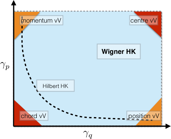
Figure 1: Schematic relationship of all semiclassical IVR propagators, see text for the discussion.

All aforementioned propagators are schematically depicted in Fig. 1. Assuming the form $\Gamma=\mathrm{diag}(\gamma_{q},\gamma_{p})$, the Wigner HK propagator covers the whole $(\gamma_{q},\gamma_{p})$ - plane. Importantly, Weyl-transforming the density operator propagated via two Hilbert space HK propagators, Eq. (1), leads to a propagator that has the same form as the Wigner HK propagator in Eq. (4) but inherits the minimal uncertainty condition, Koda (2015) which can be written as $\gamma_{q}\cdot\gamma_{p}=4$ and is represented by the blue dotted hyperbola in Fig. 1. The Hilbert space position- and momentum vV limits introduced above are characterised by $(\gamma_{q},\gamma_{p})\rightarrow(\infty,0)$ and $(\gamma_{q},\gamma_{p})\rightarrow(0,\infty)$ and are located in the lower right and upper left corners of Fig. 1, respectively. These limits preserve the minimal-uncertainty condition and are thus accessible via the Hilbert space HK propagator. In contrast, the centre- and chord vV limits are given by $(\gamma_{q},\gamma_{p})\rightarrow(\infty,\infty)$ and $(\gamma_{q},\gamma_{p})\rightarrow(0,0)$ located in the upper right and lower left corner. They can not be reached by the Hilbert space HK propagator as they disobey the minimal uncertainty condition. Overall, Fig. 1 illustrates that the Wigner HK propagator covers all important semiclassical IVR propagators that have been formulated so far.

Theoretical considerations.

The relationships in Fig. 1 can only be uncovered by a direct transform of the Hilbert space propagators into the Wigner representation. Without this explicit transform, it is natural to expect that the two versions of the HK propagator might lead to conceptually different numerical schemes. Let us consider a general expectation value, $E(t)$, of the form

$$E(t)=\mathrm{Tr}\left(\hat{A}\exp\left[-\frac{\mathrm{i}}{\hbar}\hat{H}^{+}t\right]\hat{B}\exp\left[\frac{\mathrm{i}}{\hbar}\hat{H}^{-}t\right]\right)\enspace,$$ (8)

with two Hermitian operators $\hat{A}$, $\hat{B}$ and two time-evolution operators with respect to the Hamiltonians $\hat{H}^{\pm}$. With $\hat{H}^{+}=\hat{H}^{-}$ this expression covers standard quantum expectation values and correlation functions of an observable $\hat{A}$ by identifying $\hat{B}$ with the density operator $\hat{\rho}$ or with $\hat{\rho}\cdot\hat{A}$, respectively. Further, Eq. (8) can account for non-Heisenberg time evolution with $\hat{H}^{+}\neq\hat{H}^{-}$, which appears, e.g., in optical response functions for electronic transitions. The semiclassical expression in Hilbert space, $E_{\mathrm{scl}}^{\mathrm{H}}(t)$, can be obtained straightforwardly by inserting two Hilbert space HK propagators, Eq. (1), into Eq. (8), resulting in

$$E_{\mathrm{scl}}^{\mathrm{H}}(t)=\intop\frac{\mathrm{d}z^{+}_{0}\mathrm{d}z^{-}_{0}}{(2\pi\hbar)^{2}}G_{t}(z^{+}_{0},z^{-}_{0})A^{*}(z^{+}_{t},z^{-}_{t})B(z^{+}_{0},z^{-}_{0})$$ (9)

with

$$G_{t}(z^{+}_{0},z^{-}_{0}) \equiv C_{t}(z^{+}_{0})C^{*}_{t}(z^{-}_{0})\exp\left[\frac{\mathrm{i}}{\hbar}\{S_{t}(z_{0}^{+})-S_{t}(z_{0}^{-})\}\right]$$

$$A(z_{t}^{+},z_{t}^{-}) \equiv \braket{z_{t}^{+}}{\hat{A}}{z_{t}^{-}}$$

$$B(z_{0}^{+},z_{0}^{-}) \equiv \braket{z_{0}^{+}}{\hat{B}}{z_{0}^{-}}\enspace.$$ (10)

In the Wigner representation, $E(t)$ reads

$$E(t)=\intop\mathrm{d}z\,A_{\mathrm{W}}(z)B_{\mathrm{W}}(z,t)\enspace,$$ (11)

where $A_{\mathrm{W}}(z)$ and $B_{\mathrm{W}}(z,t)$ are the Weyl symbols representing the operators $\hat{A}$ and $\exp[-\frac{\mathrm{i}}{\hbar}\hat{H}^{+}t]\hat{B}\exp[\frac{\mathrm{i}}{\hbar}\hat{H}^{-}t]$, respectively. de Almeida (1998) The corresponding semiclassical expression, $E_{\mathrm{scl}}^{\mathrm{W}}(t)$, follows directly from applying Eq. (4) to the Weyl symbol, $B_{\mathrm{W}}(z,t)$, in Eq. (11) and leads to

$$E_{\mathrm{scl}}^{\mathrm{W}}(t)\!=\!\!\intop\frac{\mathrm{d}\bar{z}_{0}\mathrm{d}\Delta z_{0}}{(2\pi\hbar)^{2}}\tilde{G}_{t}(\bar{z}_{0},\Delta z_{0})\tilde{A}_{\mathrm{W}}(\bar{z}_{t},\Delta z_{t})\tilde{B}_{\mathrm{W}}(\bar{z}_{0},\Delta z_{0})\,,$$ (12)

with the functions

$$\tilde{G}_{t}(\bar{z}_{0},\Delta z_{0}) \equiv \tilde{C}_{t}(\bar{z}_{0},\Delta z_{0})\exp\left[\frac{\mathrm{i}}{\hbar}\tilde{S}_{t}(\bar{z}_{0},\Delta z_{0})\right]$$

$$\tilde{A}_{\mathrm{W}}(\bar{z}_{t},\Delta z_{t}) \equiv \intop\mathrm{d}zA_{\mathrm{W}}(z)g(z;\bar{z}_{t},\Delta z_{t})$$

$$\tilde{B}_{\mathrm{W}}(\bar{z}_{0},\Delta z_{0}) \equiv \intop\mathrm{d}zB_{\mathrm{W}}(z)g^{*}(z;\bar{z}_{0},\Delta z_{0})\,.$$ (13)

Although the expressions for $E_{\mathrm{scl}}^{\mathrm{H}}(t)$ and $E_{\mathrm{scl}}^{\mathrm{W}}(t)$ look similar, they seem to contain different ingredients thus leading to different computation protocols. However, a careful rearrangement of all the functions in Eqs. (Theoretical considerations., Theoretical considerations.) using the transform from initial centres and chords to initial points of the trajectories, carried out in detail in the Supplement, shows that the integrands of $E_{\mathrm{scl}}^{\mathrm{H}}(t)$ and $E_{\mathrm{scl}}^{\mathrm{W}}(t)$ coincide exactly for a matrix $\Gamma$ satisfying, again, the minimal uncertainty condition $\gamma_{q}\cdot\gamma_{p}=4$. Importantly, this coincidence can be shown without the initial Weyl transform and one can, thus, conclude that the semiclassical Wigner propagator does not yield a principally new computation protocol compared to its Hilbert space version. This is the first main result of this Communication.

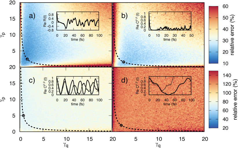
Figure 2: The error, Eq. (14), displayed as a function of $\gamma_{q}$ and $\gamma_{p}$ for the optical response function of two shifted Morse potentials (panel a) and the state-state auto-correlation function for the double-well potential in the classical, shallow, and deep tunneling regimes (panels b-d), see text. Insets compare a typical semiclassical function in question (dotted line) against the exact result (solid line). The parameters $(\gamma_{q},\gamma_{p})$ corresponding to former are marked via the black circle in the 2D error plots. Dashed line indicate the minimal uncertainty hyperbola.

Numerical investigations.

According to the theoretical considerations above, the only new aspect of the Wigner HK propagator is a mere technical flexibility in choosing the width matrix $\Gamma$ being not bound to minimal uncertainty. It remains to be checked whether this flexibility can yield a numerical advantage, which is done below based on two prototypical examples. First, the optical response function, $R(t)$, of an electronic transition between two shifted potential energy surfaces (PESs), $V_{\pm}(q)$, is investigated. Such a response function is a particular case of Eq. (8), with $\hat{A}=1$ and $\hat{B}=\hat{\rho}_{0}$, i.e. the initial state, and, being Fourier-transformed, corresponds to a vibronic spectrum in the Condon approximation. The two Hamiltonians, $\hat{H}^{\pm}$, describe the nuclear time evolution on the respective PESs, $V^{\pm}(q)$, which have the form of Morse potentials. In order to test a chemically relevant regime, $V^{+}(q)$ is chosen to be the ground state PES of the O$-$H stretch in water, with parameters taken from Ref. Paesani and Voth, 2010, whereas those for $V^{-}(q)$ are set to yield half of the harmonic frequency of $V^{+}(q)$. The upper PES is shifted by 0.2 Å and the mass of the nuclear DOF, $q$, is the reduced mass of oxygen and hydrogen, see Supplement for further details. The ground state of $V^{+}(q)$ in the Wigner representation is used as the initial state.

Second, we consider a proton in the double-well potential from Ref. Borgis, Tarjus, and Azzouz, 1992. This potential describes solvent-induced proton transfer in strongly H-bonded complexes and has a barrier height of 4 kcal/mol, which amounts to two quantum eigenstates below the barrier only. For this system, the state-state auto-correlation function, $C^{\rho\rho}(t)$, is calculated, which can be obtained from Eq. (8) by setting $\hat{A}=\hat{B}=\hat{\rho}_{0}$ and $\hat{H}^{+}=\hat{H}^{-}$. A Gaussian Wigner function, corresponding to the part of the first excited state localised in one of the wells, is taken as the initial state. Schematically, one can identify three characteristic regimes of tunneling: i) classical tunneling, where the classical trajectories can easily pass the barrier, ii) shallow tunneling, a regime where tunneling is less important but still plays a role (see also Ref. Tanaka, 2006) and iii) deep tunneling regime. In the deep tunneling regime, the chosen initial state is centred at the minimum of one of the wells (average energy of 88 % of the barrier height) and can be viewed as a superposition of the two eigenstates below the barrier. This leads to a slow Rabi-type oscillation of the probability density between the wells, which is mainly induced by tunneling. This characteristic motion is reduced when the energy of the initial state is increased, e.g., upon placing it away from the potential minimum. In the shallow tunneling regime the initial state is, thus, centred near the barrier top (130 % of the barrier energy) and strongly displaced from the minimum (820% of the barrier energy) in the classical regime.

In order to quantify the accuracy of the semiclassical treatment, the expectation values, $E_{\mathrm{scl}}(t)$, have been computed via Eq. (12) and compared against exact quantum references, $E_{\mathrm{qm}}(t)$, obtained from a second-order split-operator treatment of the Wigner propagation. We have employed 25,000 and 50,000 trajectory pairs for the first and the second example, respectively, see Supplement for further numerical details. Note that the Hilbert space HK propagator protocol is covered by Eq. (12) with $\Gamma$ fulfilling the minimal uncertainty condition. The error in the semiclassical result has been quantified as

$$\epsilon(\gamma_{q},\gamma_{p})\equiv\sqrt{\frac{\intop\mathrm{d}t|E_{\mathrm{qm}}(t)-E_{\mathrm{scl}}(t)|^{2}}{\intop\mathrm{d}t|E_{\mathrm{qm}}(t)|^{2}}}\enspace,$$ (14)

being a function of the two parameters, $\gamma_{q}$ and $\gamma_{p}$, for a diagonal matrix $\Gamma=\mathrm{diag}(\gamma_{q},\gamma_{p})$.

The error for the first example, the optical response function, is displayed in Fig. 2a), as a 2D colour plot; note that each panel has the same layout as Fig. 1. The minimal uncertainty hyperbola, that corresponds to the Hilbert space HK propagator, is indicated via the dashed line therein. The error reveals a shallow minimum ($\epsilon\approx 12\,\%$). In the inset, a representative response function, $R_{\mathrm{scl}}(t)$ (dotted line), calculated at the position indicated by a circle, is compared against the reference ,$R_{\mathrm{qm}}(t)$, (solid line) demonstrating that this error corresponds to a visually good agreement. Importantly, this shallow minimum is crossed by the minimal uncertainty line, implying that it can be accessed by the Hilbert space propagator. In contrast, the vV limits corresponding to the corners of the graph, see Fig. 1, reveal large errors confirming their numerically poor performance. It is though expected that a dramatic increase in the number of trajectory pairs will eventually yield accurate results.

Considering the accuracy of the state-state autocorrelation function of the double-well system, panels b) - d) in Fig. 2, one observes the very same behaviour for the classical tunneling regime, panel b): a shallow minimum ($\epsilon\approx 20\,\%$) is clearly visible and accessible by the minimal uncertainty line. The vV limits, in turn, show large deviations from the exact reference. The reasonable accuracy in this regime is expected, since tunneling does not play a role as the system has enough energy to pass the barrier classically. In contrast, in the shallow and deep tunneling regimes, panels c) and d), a bad accuracy of the semiclassical approximation is revealed. While the minimum of the error (with large errors of $\approx 65\,\%$) can still be recognized in the shallow tunneling regime (around the circle in panel c)), the deep tunneling regime is not accurately described on the whole $(\gamma_{q},\gamma_{p})$-plane. This is also reflected in a direct comparison of the semiclassical result, $C^{\rho\rho}_{\mathrm{scl}}(t)$, against the exact reference, $C^{\rho\rho}_{\mathrm{qm}}(t)$, see insets. Thus, the infamous breakdown of the semiclassical approximation in the deep tunneling regime Grossmann and Heller (1995); Kay (1997) is not prevented by exploiting the full flexibility in choosing the matrix $\Gamma$ and the performance is even worse in the vV limits. Overall, the numerical investigation shows that whenever the semiclassical results are accurate, the shallow error minimum is accessible via the minimal uncertainty line, i.e. via the Hilbert space HK propagator. If the semiclassical performance is bad, utilizing the broader parameter range of $\Gamma$ provided by the Wigner HK propagator does not yield an improvement.

Conclusions.

In this Communication, we have compared semiclassical Herman-Kluk and van Vleck propagators formulated in Hilbert space and in Wigner representation. It has been shown that switching to the Wigner representation yields the very same numerical protocol as in Hilbert space and is thus not beneficial. The only additional flexibility of the Wigner formulation lies in the arbitrary choice of the Gaussians’ width for the underlying coherent states being not bound to minimal uncertainty. After a careful numerical investigation for prototypical Morse and double-well potentials it has turned out that this freedom leads neither to qualitative nor quantitative improvements in performance. The overall conclusion is thus that the semiclassical Herman-Kluk propagator in Wigner representation performs exactly the same way as its state-of-the-art counterpart in Hilbert space.

The authors would like to thank Thomas Dittrich, Frank Grossmann and Oliver Kühn for fruitful and stimulating discussions. S.D.I. gratefully acknowledges the financial support by the Deutsche Forschungsgemeinschaft (IV 171/2-1).

Supplementary Material

The supplementary material contains the detailed proof that the Wigner and Hilbert-space versions of the HK propagator yield the same protocol for computing semiclassical averages. It further gives a detailed system description and elaborates on simulation strategies employed.

References

- Van Vleck (1928) J. H. Van Vleck, Proc. Natl. Acad. Sci. 14, 178 (1928).
- Littlejohn (1992) R. G. Littlejohn, J. Stat. Phys. 68, 7 (1992).
- Miller (2001) W. H. Miller, J. Phys. Chem. A 105, 2942 (2001).
- Thoss and Wang (2004) M. Thoss and H. Wang, Annu. Rev. Phys. Chem. 55, 299 (2004).
- Kay (2005) K. G. Kay, Annu. Rev. Phys. Chem. 56, 255 (2005).
- Herman and Kluk (1984) M. F. Herman and E. Kluk, Chem. Phys. 91, 27 (1984).
- Kluk, Herman, and Davis (1986) E. Kluk, M. F. Herman, and H. L. Davis, J. Chem. Phys. 84, 326 (1986).
- Kay (1994a) K. G. Kay, J. Chem. Phys. 100, 4377 (1994a).
- Kay (2006) K. G. Kay, Chem. Phys. 322, 3 (2006).
- Grossmann and Xavier (1998) F. Grossmann and A. L. Xavier, Phys. Lett. A 243, 243 (1998).
- Miller (2002a) W. H. Miller, Mol. Phys. 100, 397 (2002a).
- Miller (2002b) W. H. Miller, J. Phys. Chem. B 106, 8132 (2002b).
- Child and Shalashilin (2003) M. S. Child and D. V. Shalashilin, J. Chem. Phys. 118, 2061 (2003).
- Deshpande and Ezra (2006) S. A. Deshpande and G. S. Ezra, J. Phys. A. Math. Gen. 39, 5067 (2006).
- Heller (1981) E. J. Heller, J. Chem. Phys. 75, 2923 (1981).
- Grossmann (2013) F. Grossmann, Theoretical Femtosecond Physics, 2nd ed. (Springer International Publishing, Heidelberg, 2013).
- de Almeida (1998) A. M. O. de Almeida, Phys. Rep. 295, 265 (1998).
- Wigner (1932) E. Wigner, Phys. Rev. 40, 749 (1932).
- Hillery et al. (1984) M. Hillery, R. O’Connell, M. Scully, and E. Wigner, Phys. Rep. 106, 121 (1984).
- Berry (1977) M. V. Berry, Philos. Trans. R. Soc. A Math. Phys. Eng. Sci. 287, 237 (1977).
- Zurek (2001) W. H. Zurek, Nature 412, 712 (2001).
- Heller (1976) E. J. Heller, J. Chem. Phys. 65, 1289 (1976).
- Dittrich, Viviescas, and Sandoval (2006) T. Dittrich, C. Viviescas, and L. Sandoval, Phys. Rev. Lett. 96, 1 (2006).
- Dittrich, Gómez, and Pachón (2010) T. Dittrich, E. A. Gómez, and L. A. Pachón, J. Chem. Phys. 132, 214102 (2010).
- de Almeida, Vallejos, and Zambrano (2013) A. M. O. de Almeida, R. O. Vallejos, and E. Zambrano, J. Phys. A Math. Theor. 46, 135304 (2013).
- Koda (2015) S.-i. Koda, J. Chem. Phys. 143, 244110 (2015).
- Bondar et al. (2013) D. I. Bondar, R. Cabrera, D. V. Zhdanov, and H. A. Rabitz, Phys. Rev. A 88, 1 (2013), 1202.3628 .
- Walton and Manolopoulos (1996) A. R. Walton and D. E. Manolopoulos, Mol. Phys. 87, 961 (1996).
- Herman (1997) M. F. Herman, Chem Phys Lett 275, 445 (1997).
- Sun and Miller (1999) X. Sun and W. H. Miller, J. Chem. Phys. 110, 6635 (1999).
- Makri and Thompson (1998) N. Makri and K. Thompson, Chem. Phys. Lett. 291, 101 (1998).
- Kühn and Makri (1999) O. Kühn and N. Makri, J. Phys. Chem. A 103, 9487 (1999).
- Batista et al. (1999) V. Batista, M. Zanni, B. Greenblatt, D. Neumark, and W. Miller, J. Chem. Phys. 110, 3736 (1999).
- Skinner and Miller (1999) D. E. Skinner and W. H. Miller, Chem. Phys. 111, 10787 (1999).
- Guallar, Batista, and Miller (2000) V. Guallar, V. S. Batista, and W. H. Miller, J. Chem. Phys. 113, 9510 (2000).
- Wang, Thoss, and Miller (2000) H. Wang, M. Thoss, and W. H. Miller, J. Chem. Phys. 112, 47 (2000).
- Ovchinnikov, Apkarian, and Voth (2001) M. Ovchinnikov, V. A. Apkarian, and G. A. Voth, J. Chem. Phys. 114, 7130 (2001).
- Nakayama and Makri (2003) A. Nakayama and N. Makri, J. Chem. Phys. 119, 8592 (2003).
- Nakayama and Makri (2004) A. Nakayama and N. Makri, Chem. Phys. 304, 147 (2004).
- Tao and Miller (2009) G. Tao and W. H. Miller, J. Chem. Phys. 131 (2009), 10.1063/1.3271241.
- Herman (2014) M. F. Herman, J. Phys. Chem. B 118, 8026 (2014).
- Alemi and Loring (2015) M. Alemi and R. F. Loring, J. Phys. Chem. B 119, 8950 (2015).
- Tao and Miller (2011) G. Tao and W. H. Miller, J. Chem. Phys. 135, 024104 (2011).
- Grossmann (2006) F. Grossmann, J. Chem. Phys. 125, 014111 (2006).
- Buchholz, Grossmann, and Ceotto (2016) M. Buchholz, F. Grossmann, and M. Ceotto, J. Chem. Phys. 144, 094102 (2016).
- Koch et al. (2008) W. Koch, F. Großmann, J. Stockburger, and J. Ankerhold, Phys. Rev. Lett. 100, 230402 (2008).
- Koch et al. (2010) W. Koch, F. Großmann, J. T. Stockburger, and J. Ankerhold, Chem. Phys. 370, 34 (2010).
- Wang, Sun, and Miller (1998) H. Wang, X. Sun, and W. H. Miller, J. Chem. Phys. 108, 9726 (1998).
- Kay (1994b) K. G. Kay, J. Chem. Phys. 100, 4432 (1994b).
- Paesani and Voth (2010) F. Paesani and G. A. Voth, J. Chem. Phys. 132, 014105 (2010).
- Borgis, Tarjus, and Azzouz (1992) D. Borgis, G. Tarjus, and H. Azzouz, J. Phys. Chem. 96, 3188 (1992).
- Tanaka (2006) A. Tanaka, Phys. Rev. A 73, 1 (2006), 0601135 .
- Grossmann and Heller (1995) F. Grossmann and E. J. Heller, Chem. Phys. Lett. 241, 45 (1995).
- Kay (1997) K. G. Kay, J. Chem. Phys. 107, 2313 (1997).