Modeling NNLO jet corrections with neural networks

Abstract

We present a preliminary strategy for modeling multidimensional distributions through neural networks. We study the efficiency of the proposed strategy by considering as input data the two-dimensional next-to-next leading order (NNLO) jet $k$-factors distribution for the ATLAS 7 TeV 2011 data. We then validate the neural network model in terms of interpolation and prediction quality by comparing its results to alternative models.

07.05.Mh, 12.38.-t

1 Introduction

The calculation of higher order corrections to QCD processes, usually related to LHC measurements, requires intensive computing power and time. However, higher order corrections, such as the next-to-next leading order (NNLO), are essential in many circumstances, e.g. during the determination of parton distribution functions (PDFs) [1, 2] where theoretical predictions are computed several times during the minimization strategy adopted by the PDF fitter.

Nowadays this performance limitation is overcome by the inclusion of NNLO corrections in PDF fits through the pre-evaluation of $k$-factors, defined as the ratio between predictions at NNLO and NLO computed with the same set of PDFs. In a NNLO PDF fit the $k$-factors are multiplied to the respective NLO predictions which are evaluated using high performance techniques, such as APPLgrid [3] or APFELgrid [4], obtaining acceptable convolution timings for minimization algorithms.

The aim of this proceedings is to present a preliminary strategy based on neural networks and backpropagation to build a model for the $k$-factors multidimensional distribution, i.e. $k$-factors obtained from the ratio of differential distributions. There are two basic motivations for modeling $k$-factors. First, the possibility to provide a reliable method to interpolate and extrapolate $k$-factors for a specific process in a custom kinematic range. This is particularly useful when the computation of the exact $k$-factor requires several computing hours. Secondly, if the procedure is unbiased we have the possibility to estimate the reliability of the input $k$-factors, in terms of central values and uncertainties, by looking at the fit quality. In simple words, if an unbiased fit does not converge and produce poor statistical estimators there is a high probability that data and its uncertainties are inconsistent.

In the next sections we start by presenting the input data and strategy used here. Then we discuss the model results and validation estimators. We conclude by showing the behavior of the neural network model in an extrapolation region and comparing its results to alternative models.

2 Building the neural network model

2.1 Data

The target data selected for our exercise is the $k$-factors for the fully differential jet production at NNLO for the ATLAS 7 TeV 2011 data [8]. These results have been recently published in Ref. [5] after preliminary studies perfomed in Refs. [6, 7] and consist in a two-dimensional $k$-factors distribution binned in $(p_{T},y)$, the leading jet transverse momentum and its rapidity. Moreover, this data is reconstructed with the anti-$k_{T}$ algorithm with $R=0.4$ and the kinematic coverage is $p_{T}=[100,2000]$ GeV with $|y|<3$.

2.2 Strategy

Let us consider the full ATLAS 7 TeV 2011 dataset with $n_{\rm dat}=140$ points. In terms of notation, for each point $i=1,...,n_{\rm dat}$ we represent the corresponding $k$-factor as the pair $\{k_{i},\delta k_{i}\}$ where $k_{i}$ is the $k$-factor central value and $\delta k_{i}$ its uncertainty. The aim of the strategy proposed here is to determine a neural network model $y_{\rm pred}=\mathcal{N}(p_{T},y)$ which minimizes the loss function:

$$\chi^{2}=\sum_{i=1}^{n_{\rm dat}}(k_{i}-y_{{\rm pred},i})\sigma_{ij}^{-1}(k_{j}-y_{{\rm pred},j}),$$ (1)

where $\sigma_{ij}$ is the covariance matrix constructed from the $\delta k_{i}$ terms, which in our case is a simple diagonal matrix due to the lack of information on extra sources of correlations. The fitting procedure is then summarized by the following steps:

• We generate artificial Monte Carlo replicas from the original $k$-factor input data, by following the procedure adopted in the NNPDF framework [1]. This bootstrap procedure produces data replicas where central values are shifted following random Gaussian noise proportional to the uncertainties stored in the covariance matrix. This mechanism provides a simple way to propagate the input data uncertainty to the model, so our final model will provide predictions for uncertainties.

• The data of each MC replica is then randomly divided into two groups: training and validation. The training data is used to train the neural network through the minimization algorithm, meanwhile the validation data is used to control the quality of the fit, avoiding overlearning and underlearning.

• We adopt the stochastic gradient descent controlled by backpropagation for the minimization strategy. The stopping condition is implemented through the look-back algorithm which stores the weights and biases of the neural network at the minimum of the validation error function.

2.3 Algorithm settings

We have implemented the above strategy using Keras v1.1.1 [9] with Tensorflow v1.0.0 [10] backend. This choice is motivated by the great advantages provided by these codes like fast prototyping and high flexibility when testing several optimization algorithms and neural network architectures.

The final settings adopted in this exercise have been obtained through an intensive hyperparameter grid search, where we tested the quality of the loss function of the training and validation sets over several configurations. Our current best setup consists in a multilayer perceptron network with architecture 2-5-3-1 where the hidden layers have hyperbolic tangent activation functions and the last layer is linear. We have two input nodes that take pairs of points $(p_{T},y)$ and one single output node which represents the $k$-factor prediction. In terms of training and validation split we divide the original data into 50%-50% random sets for each MC replica. We use as optimizer the RMS propagation with learning rate of $l_{r}=0.01$ associated to the look-back stopping algorithm on 100k epochs. Using this setup a single replica fit usually takes 5 minutes to complete the minimization in a single core.

Finally, we remove replica outliers by applying a $\chi^{2}$ veto condition in which a neural network replica is accepted if its $\chi^{2}$ to the original dataset is within 4-$\sigma$ of the average over all replicas. The results presented in the next sections are based on a final set of $n_{\rm rep}=500$ replicas.

2.4 Results and validation

In the left plot of Figure 1 we show the distribution of the total $\chi^{2}$/dof to the original input data for each neural network replica. The shape and central value of this distribution confirm the good quality of the trained model. On the right plot of the same figure, the distribution of stopping epochs is presented for each replica. In the current setup, less than 25% of the total number of replicas stops at the maximum number of iterations, while the other replicas stop uniformly between 1k and 90k iterations.

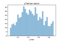
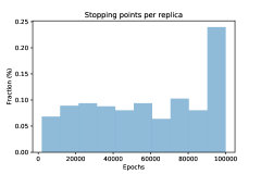
Figure 1: On the left, the $\chi^{2}$/dof for the full dataset for each replica. On the right, the distribution of stopping epoch for each replica.

In Figure 2 we show the training and validation $\chi^{2}$/dof distributions for all replicas. The left plot shows the histogram distribution meanwhile on the right we have the scatter plot of the same quantities, i.e. the blue points, and the red marker represents the average value for both quantities. Also here, the shape and peak values of both distributions are close to each other and in average within the $\chi^{2}$/dof interval $[1.8,2.5]$, which suggests that the model is trained satisfactorily.

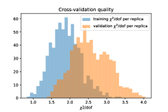
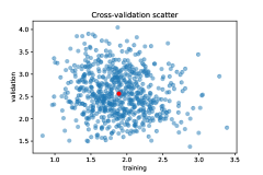
Figure 2: The training and validation $\chi^{2}$/dof distribution histogram (on the left) and scatter plot (on the right). The average value for training and validation is shown by the red marker in the scatter plot.

The left plot in Figure 3 shows the final results for the neural network model. The black points are the input $k$-factors, following the ATLAS 7 TeV 2011 data kinematics, divided by rapidity bins. The blue line and band are respectively the neural network central value and uncertainty prediction. From the plots we conclude that the neural network model is performing well in representing the shape variation of $k$-factors in the $(p_{T},y)$ bins. For comparison reasons, on the right side of the same figure, we plot predictions for the same input data using a 2nd degree two-dimensional polynomial parametrization (red line) and a bivariate cubic spline (yellow band) both trained with generalized least-square minimization. In Table 1 we computed the total $\chi^{2}$/dof to the original input data for each model.

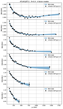
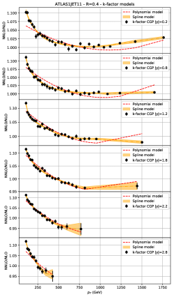
Figure 3: Model results compared to the input $k$-factors for the ATLAS 7 TeV 2011 data. On the left, the $k$-factors (black points) separated in bins of rapidity with the neural network model central value and uncertainty predictions. On the right, similar results for the polynomial (in red dashed lines) and the spline (yellow band and line) models.

First of all, we conclude that the polynomial model, even if it is simpler and faster to fit, usually requires a long period of fine tune of its degree and configuration. We observe that with our input data, polynomial predictions are not sufficiently compatible with data. On the other hand, the spline model provides a good interpolation of the input data, however as we will see in the next section we have to select a model which is stable over kinematics variations, including the extrapolation region. Furthermore, it is important to highlight that the polynomial and spline models will require special fine tunes when generalizing the problem to higher dimensions, meanwhile for the neural network model we will have just to increase the number of input nodes and perform the hyperparameter grid search.

Model	$\chi^{2}$/dof
Neural-network	0.93
Spline	0.66
Polynomial	5.92

Table 1: Total $\chi^{2}$/dof for the neural network model 2.3, the bivariate cubic spline and the 2nd degree two-dimensional polynomial.

3 Extrapolating predictions

In order to test the extrapolation of all models presented in the previous section we have computed predictions using the kinematic settings of ATLAS 7 TeV 2010 [11]. The only difference between this dataset and the ATLAS 7 TeV 2011 used to train the models consists in a wider range and binning of $(p_{T},y)$, in particular $|y|<4.4$ and $p_{T}=[20,1500]$ GeV. The ATLAS 7 TeV 2011 and 2010 have exactly the same theoretical setup: $\sqrt{s}=7$ TeV and $R=0.4$ anti-$k_{t}$ jet reconstruction radius and algorithm.

Figure 4 illustrates the predictions for the neural network model (left side) and the spline and polynomial (right side) for the ATLAS 7 TeV 2010 in $(p_{T},y)$ bins. As we do not have yet available the final exact $k$-factors for this experiment, in order to compute the final total $\chi^{2}$/dof for each model, we can judge the quality of extrapolation prediction by looking at central values and uncertainties provided by each model. The most stable behavior among all the three different models is the one provided by the neural network, which simulates the typical shape steepness when increasing the rapidity and reducing the $p_{T}$. The spline model fails to predict such regions, in particular we highlight the presence of negative predictions and large uncertainties. We also observe that uncertainties oscillate if the requested $(p_{T},y)$ bin is too different from the original input data.

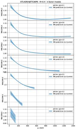
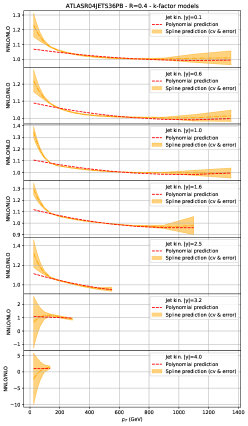
Figure 4: Same as Figure 3 for ATLAS 7 TeV 2010 [11].

4 Conclusions and outlook

From this exercise we conclude that there are at least two clear advantages in using neural networks to model multidimensional distributions: no need for a model definition, neural networks can simulate every function; the possibility to interpolate and extrapolate multidimensional distributions from two or higher dimensions easily.

We outlook that this model could be applied in many distributions provided by Monte Carlo generators, by at least removing the requirement of rebinning. We also highlight that the such model could provide a quantitative measurement of the input data consistency.

S.C. is supported by the HICCUP ERC Consolidator grant (614577).

References

- [1] R. D. Ball et al. [NNPDF Collaboration], JHEP 1504 (2015) 040 doi:10.1007/JHEP04(2015)040 [arXiv:1410.8849 [hep-ph]].
- [2] R. D. Ball et al., Nucl. Phys. B 867 (2013) 244 doi:10.1016/j.nuclphysb.2012.10.003 [arXiv:1207.1303 [hep-ph]].
- [3] T. Carli, D. Clements, A. Cooper-Sarkar, C. Gwenlan, G. P. Salam, F. Siegert, P. Starovoitov and M. Sutton, Eur. Phys. J. C 66 (2010) 503 doi:10.1140/epjc/s10052-010-1255-0 [arXiv:0911.2985 [hep-ph]].
- [4] V. Bertone, S. Carrazza and N. P. Hartland, Comput. Phys. Commun. 212 (2017) 205 doi:10.1016/j.cpc.2016.10.006 [arXiv:1605.02070 [hep-ph]].
- [5] J. Currie, E. W. N. Glover and J. Pires, Phys. Rev. Lett. 118 (2017) no.7, 072002 doi:10.1103/PhysRevLett.118.072002 [arXiv:1611.01460 [hep-ph]].
- [6] J. Currie, A. Gehrmann-De Ridder, E. W. N. Glover and J. Pires, JHEP 1401 (2014) 110 doi:10.1007/JHEP01(2014)110 [arXiv:1310.3993 [hep-ph]].
- [7] S. Carrazza and J. Pires, JHEP 1410 (2014) 145 doi:10.1007/JHEP10(2014)145 [arXiv:1407.7031 [hep-ph]].
- [8] G. Aad et al. [ATLAS Collaboration], JHEP 1502 (2015) 153 Erratum: [JHEP 1509 (2015) 141] doi:10.1007/JHEP02(2015)153, 10.1007/JHEP09(2015)141 [arXiv:1410.8857 [hep-ex]].
- [9] F. Chollet. keras. https://github.com/fchollet/keras, 2015.
- [10] M. Abadi, et al. TensorFlow: Large-scale machine learning on heterogeneous systems, 2015. Software available from tensorflow.org.
- [11] G. Aad et al. [ATLAS Collaboration], Eur. Phys. J. C 71 (2011) 1512 doi:10.1140/epjc/s10052-010-1512-2 [arXiv:1009.5908 [hep-ex]].