Chandra Phase-Resolved Spectroscopy of the High Magnetic Field Pulsar B1509$-$58

Abstract

We report on a timing and spectral analysis of the young, high magnetic field rotation-powered pulsar (RPP) B1509$-$58 using Chandra continuous-clocking mode observation. The pulsar’s X-ray light curve can be fit by the two Gaussian components and the pulsed fraction shows moderate energy dependence over the Chandra band. The pulsed X-ray spectrum is well described by a power law with a photon index 1.16(4), which is harder than the values measured with RXTE/PCA and NuSTAR. This result supports the log-parabolic model for the broadband X-ray spectrum. With the unprecedented angular resolution of Chandra, we clearly identified off-pulse X-ray emission from the pulsar, and its spectrum is best fit by a power law plus blackbody model. The latter component has a temperature of $\sim$0.14 keV with a bolometric luminosity comparable to the luminosities of other young and high magnetic field RPPs, and it lies between the temperature of magnetars and typical RPPs. In addition, we found that the nonthermal X-ray emission of PSR B1509$-$58 is significantly softer in the off-pulse phase than in the pulsed phase, with the photon index varying between 1.0 and 1.8 and anticorrelated with the flux. This is similar to the behavior of three other young pulsars. We interpreted it as different contributions of pair-creation processes at different altitudes from the neutron star surface according to the outer-gap model.

1. Introduction

Pulsars are fast-rotating neutron stars. Most of them spin down steadily, converting their rotational energy into electromagnetic radiation and particle outflows. This class of pulsars is thus known as rotation-powered pulsars (RPPs). They typically have spin periods of $\sim$0.1–10 s and period derivatives of $\sim 10^{-12}$–$10^{-17}$ s s^-1, implying magnetic fields of $B\sim 10^{11}$–$10^{13}$ G. Thanks to the revolution of astronomical instrumentation in the past two decades, several subtypes of pulsars have been discovered, and they occupy different regions in the $P$-$\dot{P}$ diagram. Magnetars are an extreme group of pulsars with long spin periods of 2–12 s and strong magnetic fields of $10^{14}$–$10^{15}$ G inferred from the spin-down rate. They are remarkable for their energetic burst activities and high X-ray luminosities (see review by Mereghetti, 2008; Mereghetti et al., 2015). The theoretical interpretation is that the energetic features are powered by the dissipation and decay of a strong magnetic field (Thompson & Duncan, 1995, 1996), although the mechanism that converts the magnetic energy into the surface heating remains an open question (see Turolla et al., 2015; Beloborodov & Li, 2016). Moreover, recent discoveries blurred the boundary between magnetars and RPPs. The low field magnetars SGR 0418+5729 and Swift J1822.3$-$1606 have spin-down-inferred dipole magnetic fields of $6\times 10^{12}$ G and $1.4\times 10^{13}$ G, respectively, comparable to typical RPPs (Rea et al., 2010, 2013; Scholz et al., 2012). Furthermore, the discovery of magnetar-like bursts of high magnetic field RPPs J1846$-$0258 with $B=4.9\times 10^{13}$ G (Gavriil et al., 2008; Ng et al., 2008), and J1119$-$6127 with $B=4.1\times 10^{13}$ G (Archibald et al., 2016; Göğüş et al., 2016) also challenges the division between these two classes of neutron stars. To interpret the fact that magnetar and high magnetic field RPPs share similar behaviors, a unified model has been proposed (Perna & Pons, 2011; Viganò et al., 2013) based on the magneto-thermal evolution (e.g., Pons & Geppert, 2007).

Because pulsars are born as hot objects, young pulsars provide good targets for measuring the thermal emission and testing the above theory. There are only three high magnetic field ($B>10^{13}$ G) RPPs younger than 2000 years: PSRs B1509$-$58, J1846$-$0258, and J1119$-$6127. PSR B1509$-$58 (catalog ) (hereafter B1509) is the only one for which the thermal emission has not been studied. To complete the sample, we carry out a measurement of the surface temperature of B1509 with the Chandra X-ray Observatory in this study.

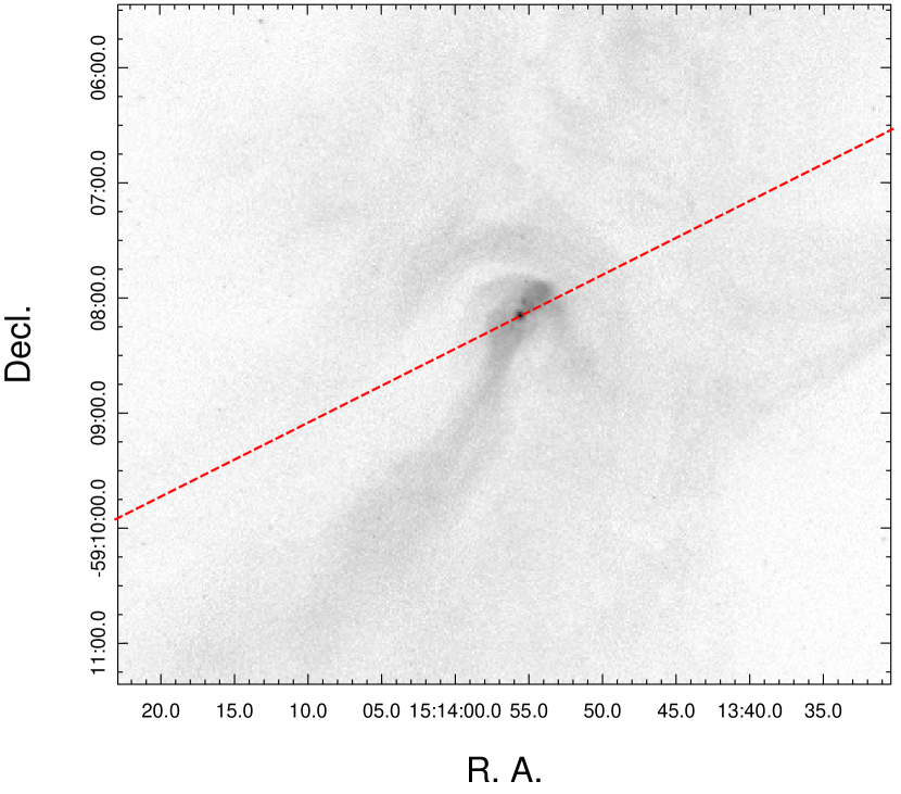
Figure 1.— Chandra X-ray image of B1509 and its PWN in MSH 15-52 in the 0.5–7 keV band. All the X-ray events are projected onto the red dashed line in the CC mode observation to form a 1D image. This image is created by accumulating all the archival observations with Chandra ACIS-I and operated in the TE mode.

B1509 has a spin period of 150 ms, which was first discovered in X-rays with the Einstein Observatory (Seward & Harnden, 1982). It is embedded in a bright supernova remnant MSH 15$-$52 (Mills et al., 1960). Radio pulsations were detected subsequently, and a large period derivative of $\sim 1.5\times 10^{-12}$ s s^-1 was also confirmed (Manchester et al., 1982; Weisskopf et al., 1983). This implies a dipole field of $B=1.5\times 10^{13}$ G, which is higher than that of SGR 0418+5729. The radio pulse profile shows a sharp peak, while the X-ray profile has a single, broad, and asymmetric peak and lags the radio peak by about one quarter of the cycle (Kawai et al., 1991). The broad X-ray pulse profile was conventionally described by two Gaussian components (Cusumano et al., 2001; Ge et al., 2012). Using 11 years of radio timing observations, the detailed spin-down evolution suggests a characteristic age of 1700 years (Kaspi et al., 1994). The distance is $5.2\pm 1.4$ kpc estimated from the Hi measurement (Gaensler et al., 1999).

B1509 is associated with a bright pulsar wind nebula (PWN). The high-resolution Chandra image in Figure 1 shows a bright jet in the southeast and a semicircular arc 30″ north of the pulsar (Gaensler et al., 2002). A few bright clumps were found in the northwest and are occasionally seen in the southeast, indicating the turbulent nature of the flows near the pulsar (DeLaney et al., 2006). Moreover, an inner ring-like structure with a 10″ radius surrounding the pulsar was found, which may correspond to the wind termination shock (Yatsu et al., 2009). Although Chandra can resolve B1509 from the surrounding PWN, its surface temperature has never been determined because the emission is too bright, such that the spectrum was heavily distorted by the pile-up effect. (Gaensler et al., 2002).

Using the EXOSAT, Ginga, and SIGMA data, Greiveldinger et al. (1995) determined a hydrogen column density of the PWN of $N_{\rm H}\approx 9.5\times 10^{21}$ cm^-2 and concluded that the pulsar had a harder emission than its surrounding nebula. The pulsed spectrum obtained with the RXTE can be well fit by a power law (PL) with a photon index $\Gamma=1.36\pm 0.01$. The off-pulse spectrum, which was dominated by the surrounding nebular emission due to the poor spatial resolution, shows a much softer PL with $\Gamma=2.215\pm 0.005$ (Marsden et al., 1997). A pulse phase-resolved spectral analysis showed that $\Gamma$ remains stable during the pulsed phase, such that the spectra of the two components of the pulse shape are indistinguishable (Rots et al., 1998). Ge et al. (2012) presented a more comprehensive phase-resolved spectral analysis using 15 years of RXTE data with a total exposure time of $\sim$578 ks. They treated the 0.2 cycles off-pulse emission as the background and found that $\Gamma$ increases from 1.33 to 1.47 as the flux decreases. In addition, the photon indices observed with LECS, MECS, and PDS onboard BeppoSAX are significantly different and the 0.1–300 keV broadband spectrum is better fit by a curved log-parabolic model than by a single PL (Cusumano et al., 2001). The recent NuSTAR observation provides supporting evidence for the log-parabolic model (Chen et al., 2016), although the parameters slightly deviate from those determined from BeppoSAX. However, both the PL and the log-parabolic models are equally good in a detailed phase-resolved analysis.

In this paper, we present a detailed phase-resolved analysis of the X-ray emission of B1509, using high temporal resolution data taken with Chandra. We describe the observations in Section 2, including a new observation made with the ACIS-S in the continuous-clocking (CC) mode and an archival observation made with the High Resolution Camera (HRC). Section 3 presents the data analysis and results, including the detection of the off-pulse emission from the neutron star, the on- and off-pulse spectra, and the phase-resolved analysis. We then discuss the results in Section 4 and give a summary in Section 5.

2. Observations and Data Reduction

A new observation of B1509 was made with Chandra on 2013 March 29 with a total exposure of 60.1 ks ObsID 14805 (catalog ADS/Sa.CXO#obs/14805). The ACIS-S CCD array was operated in the CC mode with a high timing resolution of 2.85 ms, such that the pile-up is negligible. Note that the CC mode observation only has one-dimensional spatial information since the events are collapsed along CCD columns into a line. The roll angle of the telescope was carefully chosen to avoid the bright features of the PWN, including the jet and the clumps, from falling onto the same CCD column as the pulsar (see Figure 1). We also used the archival observation ObsID 5515 (catalog ADS/Sa.CXO#obs/5515) made with the HRC-I on 2015 June 13 to verify the detection of the off-pulse emission.

We reprocessed both the ACIS-S and HRC data using the task chandra_repro in the Chandra Interactive Analysis of Observations (CIAO) v4.8 with the most recent calibration database (CALDB) 4.7.0. To perform an accurate timing analysis, we corrected all photon arrival times to the barycenter of the solar system with the CIAO tool axbary, based on the JPL solar system ephemeris DE405. We examined the background light curve and found no significant background flares in either observations. Therefore, all the time spans with exposures of 59.9 ks for ACIS-S CC mode data and 44.9 ks for HRC data were used in this analysis.

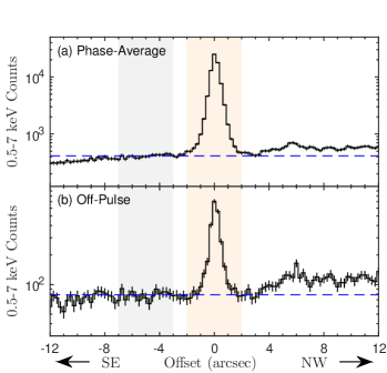
Figure 2.— Projected photon distribution of B1509 obtained with the Chandra CC mode observation in the 0.5–7 keV energy range (see Figure 1). Data were collected from (a) the phase-averaged and (b) off-pulse phases. Positive offset is defined as the northwest direction from the pulsar. The orange shaded area indicates the source region and the gray shaded area indicates the background region. The blue dashed line is the mean background value.

3. Data Analysis and Results

3.1. Radio Ephemeris

We used the pulsar ephemeris obtained with the Parkes Observatory, which is a part of the timing program for Fermi (Weltevrede et al., 2010). A total of 88 times of pulse arrivals (TOAs) between MJD 54220 and MJD 56512 were used to generate the short time-baseline ephemeris. We then used the TEMPO2 package to fit the TOAs with the rotational frequency and its first two time-derivatives. Because of the significant timing noise of B1509, we furthermore used the FITWAVES algorithm (Hobbs et al., 2004), which employs the sinusoidal curves instead of higher-order polynomials, to fit the residuals. We used five harmonics to whiten the timing noise, and the final rms residual is 1.4 ms. The dispersion measure was set to $252.5\pm 0.3$ pc cm^-3.

3.2. Source and Background Selection

Unlike previous studies that treated the off-pulse X-ray emission as the background, the superb angular resolution of Chandra can minimize the contamination from the surrounding PWN, enabling us to investigate the off-pulse emission. The source selection criterion for the CC mode observation, which is indicated by the orange shaded area in Figure 2, is defined as a 4″ wide box centered on B1509. The point spread function (PSF) generated by the raytrace simulation tool ChaRT suggested that our source selection region contains more than 95% of the source flux. We obtained a total of $\sim$82,000 counts in 0.5–7 keV.

In the projected count profile in Figure 2(a), a bump is clearly seen on the northwest side of the pulsar. This is likely related to the bright clumps in the PWN (Gaensler et al., 2002; DeLaney et al., 2006). To avoid overestimating the background level, we chose a 4″ wide region with 1″ separation from the source region in the southeast as the background (indicated as the gray shaded area in Figure 2) in the analysis. We also tried using the average of both sides as the background in the spectral analysis and found that the results are similar.

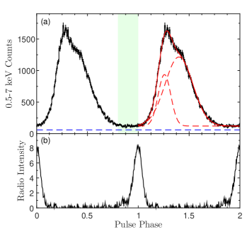
Figure 3.— (a) Folded pulse profile of B1509 in 0.5–7 keV. We divided the photons into 128 bins per spin period and plotted two cycles. The green shaded region defines the off-pulse phase. The blue dashed line denotes the background level. The red solid line is the best-fit two-Gaussian model, with the two components shown by the red dashed lines. (b) The radio pulse profile in an arbitrary unit. The two profiles are aligned in phase, with phase zero corresponding to the radio peak.

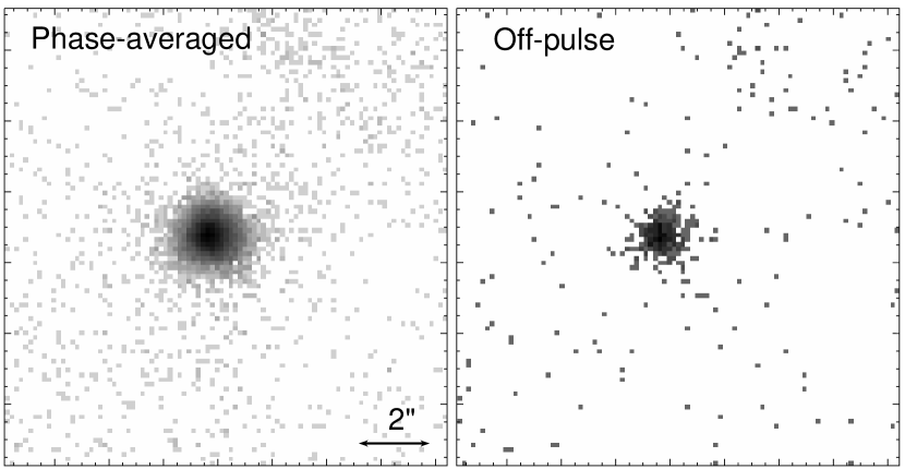
Figure 4.— The HRC phase-averaged and off-pulse images of B1509 (see Figure 3 for the definition of the phase range). The off-pulse emission is obviously a point source consistent with the phase-averaged emission.

3.3. Timing Analysis

We folded the photon arrival times of the CC mode observation according to the radio timing ephemeris. The X-ray and radio profiles are shown in Figure 3 and the radio peak is defined as phase zero. The X-ray profile shows a single, broad, and asymmetric peak, with a fast rise and a relatively slower decay, and it lags the radio peak by more than 0.2 cycles. To investigate the off-pulse emission, we collected all X-ray photons at the pulse minimum, defined as phase 0.8–1.0 (see Figure 3), and plot the count distribution along the projected direction in Figure 2(b). An excess of a width comparable to the model PSF is clearly seen at the pulsar position, indicating that the pulsar is still much brighter than the surrounding during the off-pulse phase. We furthermore confirmed the detection of the off-pulse emission by examining the archival HRC off-pulse image (see Figure 4). We searched the period of HRC data with the $H$-test algorithm (de Jager et al., 1989) since the observation is not covered by the radio ephemeris, and then folded the photon arrival times according to the best-determined period. The pulse profile is consistent with the CC mode profile in Figure 3. The off-pulse HRC image is fully consistent with the pulsed image and the model PSF.

Table 1Best-fit Parameters for the Pulse profile of B1509 Observed with Chandra in Different Energy Bands.

Parameter	0.5–7 keV	0.5–1.7 keV	1.7–2.7 keV	2.7–4.0 keV	4.0–7.0 keV
$\mu_{1}$	0.257(1)	0.252(3)	0.260(3)	0.261(3)	0.260(3)
$\sigma_{1}$	0.062(2)	0.063(5)	0.058(3)	0.068(4)	0.062(2)
$\mu_{2}$	0.399(3)	0.398(9)	0.395(4)	0.409(8)	0.398(5)
$\sigma_{2}$	0.137(2)	0.136(5)	0.140(3)	0.137(4)	0.137(2)
F$(\rm{A}_{1})$	0.25(1)	0.25(4)	0.22(2)	0.30(3)	0.25(2)
PFarea	0.87(2)	0.80(5)	0.87(3)	0.90(5)	0.90(4)
$\chi^{2}/dof$	183.3/121	38.6/43	44.1/43	71.1/43	47.6/43

Previous studies found that the pulse profile can be fit with two Gaussian components (Kuiper et al., 1999; Cusumano et al., 2001; Ge et al., 2012). Moreover, the leading narrower peak contributes less emission at higher energy bands (Ge et al., 2012), and even vanishes in the 30 MeV–1 GeV band observed with the Fermi Large Area Telescope (Kuiper & Hermsen, 2015). The two-Gaussian function is expressed as

$$f(\phi)=C+\frac{A_{1}}{\sqrt{2\pi}\sigma_{1}}e^{-\frac{1}{2}\left(\frac{\phi-\mu_{1}}{\sigma_{1}}\right)^{2}}+\frac{A_{2}}{\sqrt{2\pi}\sigma_{2}}e^{-\frac{1}{2}\left(\frac{\phi-\mu_{2}}{\sigma_{2}}\right)^{2}}$$ (1)

where $f(\phi)$ is the X-ray counts at phase $\phi$, $C$ is a constant term representing the off-pulse emission, and $\mu$ and $\sigma$ are the peak location and the width of individual Gaussian functions. The normalization factor for each Gaussian function is $A/\sqrt{2\pi}\sigma$, where $A$ is the area below the individual Gaussian function. We fit the Chandra 0.5–7 keV profile with the above function and obtained an acceptable result with a reduced $\chi^{2}$ value of 1.5. The two Gaussian components peak at phase $0.257\pm 0.001$ and $0.399\pm 0.003$, respectively. Their phase difference is consistent with those measured with RXTE in 2–5 keV (Ge et al., 2012) and BeppoSAX MECS in 1.6–10 keV (Cusumano et al., 2001). The best-fit model and the individual components are shown in the second cycle of Figure 3 (a). The narrower component contributes $25.1\pm 1.3$ % of the total pulsed emission, which is in an agreement with the previous results (Kuiper et al., 1999; Cusumano et al., 2001). The best-fit parameters are listed in Table 1.

To investigate the energy dependence of the pulse profile, we divided the X-ray photons into four energy bands: 0.5–1.7, 1.7–2.7, 2.7–4, and 4–7 keV, with a similar number of counts in each band. We then folded the X-ray light curves with 50 phase bins in each energy band, and fit the profiles with the double Gaussian function. The background-subtracted pulse profiles, the best-fit two-Gaussian functions, and the profile of each Gaussian component are shown in Figure 5. The best-fit parameters, including $\mu_{1}$, $\mu_{2}$, $\sigma_{1}$, and $\sigma_{2}$ are listed in Table 1.

We noted that all fits have $\chi^{2}_{\nu}\sim 1.0$ except for fit at 2.7–4 keV, which has $\chi^{2}_{\nu}\sim 1.6$. This could be contributed by the bump between the two Gaussian peaks at phase 0.4–0.45. We further divided the bands into more subbands and performed the same analysis, and found that the profile occasionally cannot be fit well. In these cases, the second peak jitters slightly and results in the bump structure around the best-fit second peak. Therefore, we concluded that the local structure is likely a statistical fluctuation. The parameters $\mu$ and $\sigma$ for each component do not significantly vary with respect to energy and are consistent with the results obtained in the similar energy bands of previous studies (Cusumano et al., 2001; Ge et al., 2012). The flux ratio $F(A_{1})=A_{1}/(A_{1}+A_{2})$ varies between $\sim$0.2 and $\sim$0.3 and also shows no significant energy dependency either. This means that the pulse profile does not change evidently throughout the Chandra energy range, although the strength of the narrower peak decreases as the energy increases beyond the Chandra band (Kuiper & Hermsen, 2015).

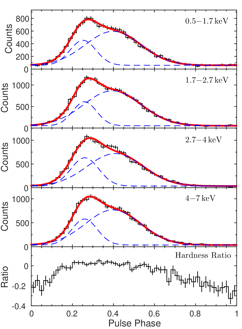
Figure 5.— Pulse profiles of B1509 in four energy bands (0.5–1.7, 1.7–2.7, 2.7–4, and 4–7 keV) and the hardness ratio obtained with Chandra. The hardness ratio is defined as $(\rm{H}-\rm{S})/(\rm{H}+\rm{S})$, where $H$ is the counts in 2.7–7 keV, and $S$ is the counts in 0.5–2.7 keV. The best-fit model is marked by thick red lines, and the individual Gaussian components are shown by blue dashed lines.

Another important derived parameter is the pulsed fraction. This can be estimated either from the pulsed and total area below the pulse profile (PF_area) or by the root mean square (rms) method based on Fourier decomposition (Dib et al., 2009; Chen et al., 2016). The variations in PF obtained with both methods are shown in Figure 6. We found that PF shows an increasing trend with energy, indicating that the off-pulse emission contributes more in the soft X-ray band. This gives us a hint of the softening at the pulse minimum. The flux ratio $F(A_{1})$ and PF_area are listed in Table 1. The pulsed fraction obtained with Chandra HRC observation is $\sim 0.88$ (Chen et al., 2016), which is consistent with the mean value of these four energy bands.

The hardness ratio (HR), which is defined as

$$\rm HR=\frac{H-S}{H+S}\ ,$$ (2)

where $H$ is the hard X-ray counts and $S$ is the soft X-ray counts, can provide us crude information of the spectral behavior. Here we defined $S$ as the number of counts in 0.5–2.7 keV, which is the combination of the two softest bands in the analysis above, and $H$ as the number of counts in 2.7–7.0 keV. The phase variation in HR is shown in the bottom panel of Figure 5. It is clear that the ratio is stable at HR$\gtrsim 0$ between phase 0.15 and 0.65, indicating that the spectral behaviors of these two Gaussian peaks are the same. Moreover, the HR drops to negative values at the off-pulse phases, which also supports the softening indicated by the PF. This could be caused by a change in PL index with the pulse phase, or by the presence of an additional soft component (see Section 3.4 below).

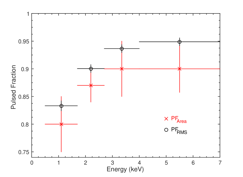
Figure 6.— Pulsed fraction of B1509 observed with Chandra ACIS estimated by the RMS method (black circles) and the area method (red crosses)

3.4. Spectral Analysis

3.4.1 Phase-averaged Spectrum

We first extracted the spectrum from the source and background regions described in Section 3.2. The spectral fitting was carried out with the Sherpa package. We performed the spectral fitting over the 0.5–7 keV range and grouped the photons to at least 50 counts per energy bin. We fit a PL with the absorption model tbnew and set the solar abundance according to Wilms et al. (2000). The best-fit parameters are $N_{\rm{H}}=(1.43\pm 0.04)\times 10^{22}$ cm^-2, $\Gamma=1.18\pm 0.03$, and $\chi_{\nu}^{2}=0.98$, where all reported uncertainties are in the 90 % confidence interval. The 0.5–7 keV absorbed flux is $(2.0\pm 0.1)\times 10^{-11}$ erg cm^-2 s^-1. The $N_{\rm{H}}$ value is significantly higher than those previously reported using Chandra (Gaensler et al., 2002), XMM-Newton (Schöck et al., 2010), and BeppoSAX (Cusumano et al., 2001) observations. This could be attributed to the different choice of abundance table and absorption model. We also followed previous studies to use the abundances by Anders & Grevesse (1989) with the absorption model phabs, and obtained $N_{\rm{H}}=(9.7\pm 0.3)\times 10^{21}$ cm^-2, which agrees well with the Chandra and BeppoSAX values (Cusumano et al., 2001; Gaensler et al., 2002), and is $15\pm 4$ % smaller than the abundance determined by Schöck et al. (2010).

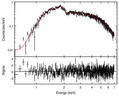
Figure 7.— Pulsed spectrum of B1509. The data points in the top panel showed the 0.5–7 keV spectrum of B1509, and the red curve corresponds to the best-fit PL model. The bottom panel shows the fit residual.

Table 2Best-fit Parameters for the PL and Logpar Models of the Pulsed X-ray Spectrum of B1509.

Parameter	Chandra		NuSTAR		BeppoSAX
	PL	Logpar	PL	Logpar	PL
$N_{\rm{H}}$ ($10^{22}$ cm-2)	1.57(6)	1.5(1)	0.95(fixed)	0.95(fixed)	0.91(fixed)
$\Gamma$	1.18(4)	$\cdots$	1.386(7)	$\cdots$	$\cdots$
$\alpha$	$\cdots$	0.9(3)	$\cdots$	1.16(5)	0.96(8)
$\beta$	$\cdots$	0.2(2)	$\cdots$	0.11(2)	0.16(4)
$\chi^{2}/dof$	352.7/388	350.4/387	278/254	254/253	26.6/36

Note. — The NuSTAR and BeppoSAX results of pulsed spectra are listed for reference (Cusumano et al., 2001; Chen et al., 2016).

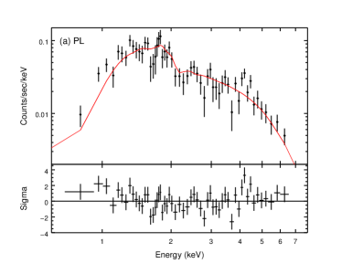
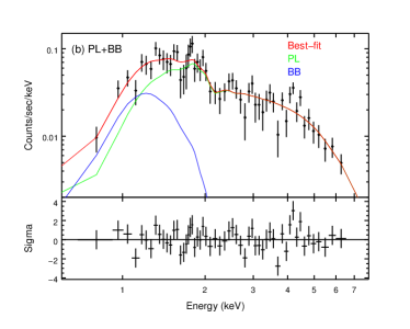
Figure 8.— The Chandra off-pulse (phase 0.8–1.0) spectrum of B1509 fit by (a) a PL model and (b) a PL+BB model.

3.4.2 Pulsed Spectrum

We furthermore extracted the 0.5–7 keV pulsed spectrum by subtracting the off-pulse emission from the pulsed one (phase 0–0.7) to compare our result with previous studies (Cusumano et al., 2001; Chen et al., 2016). After the background subtraction, we collected $\sim$71,000 photons. Following the same choice of abundance table and absorption model, the pulsed spectrum can be well fit with an absorbed PL, and the best-fit model with residuals is shown in Figure 7. The best-fit parameters are $N_{\rm{H}}=(1.57\pm 0.06)\times 10^{22}$ cm^-2, $\Gamma=1.18\pm 0.04$, and $\chi^{2}_{\nu}=0.91$. The absorbed X-ray flux within 0.5–7 keV is $(2.5\pm 0.2)\times 10^{-11}$ erg cm^-2 s^-1, where the phase duration is accounted for hereafter. The parameters are consistent with those of the phase-averaged spectrum above because the X-ray emission is dominated by the pulsed emission.

The photon index we obtained agrees with the value determined with BeppoSAX MECS ($\Gamma=1.19\pm 0.04$, Cusumano et al., 2001), but it is significantly lower than the those RXTE ($\Gamma\approx 1.35)$) and NuSTAR ($\Gamma=1.386\pm 0.07$) values (Rots et al., 1998; Ge et al., 2012; Chen et al., 2016). Previous studies found that the photon index of B1509 could change with energy, and the log-parabola model (logpar) gives a better fit to the broadband spectrum (Cusumano et al., 2001; Chen et al., 2016). The mathematical form of the logpar model is

$$f(x)=A\left(\frac{x}{x_{\rm{ref}}}\right)^{-\alpha-\beta\log(x/x_{\rm{ref}})},$$ (3)

where $x$ is the energy in units of keV and $x_{\rm{ref}}$ is the reference energy frozen at 1 keV, $\alpha$ is the photon index at $x_{\rm{ref}}$, $\beta$ is the curvature term, and $A$ is the normalization. We employed this model to fit the pulsed Chandra spectrum, and the best-fit parameters are listed in Table 2. We note that the logpar model does not significantly improve the fit, and $\alpha$ is consistent with $\Gamma$ in the PL model. In addition, $\beta$ is not well determined, indicating that the spectral curvature is not obvious over the Chandra energy range. We also show the NuSTAR and BeppoSAX results in Table 2 for comparison. It is clear that $\alpha$ and $\Gamma$ determined from Chandra are consistent with the $\alpha$ determined with NuSTAR and BeppoSAX.

Table 3Best-fit Parameters for the Simultaneous Fits to the Pulsed and Off-pulse Spectra of B1509 with Different Statistics and Models.

Model		Parameter	$\chi^{2}$ Statistic	Cash Statistic
Pulsed	Off-pulse
PL	PL	$N_{\rm{H}}$ ($10^{22}$ cm-2)	1.54(6)	1.55(6)
		$\Gamma_{\textrm{pulsed}}$	1.16(3)	1.16(3)
		$\Gamma_{\textrm{off-pulse}}$	1.85(15)	1.78(13)
		statistic$/dof$	430.9/442	1000.7/883
PL	PL+BB	$N_{\rm{H}}$ ($10^{22}$ cm-2)	1.57(6)	1.58(6)
		$\Gamma_{\textrm{pulsed}}$	1.18(4)	1.18(3)
		$\Gamma_{\textrm{off-pulse}}$	$1.5^{+0.2}_{-0.3}$	1.4(2)
		$kT$ (keV)	$0.17_{-0.05}^{+0.06}$	$0.16_{-0.04}^{+0.05}$
		$R_{\rm{BB}}$ (km)	$9_{-5}^{+38}$	$10_{-5}^{+39}$
		statistic$/dof$	413.7/440	979.9/881
PL	PL+BB	$N_{\rm{H}}$ ($10^{22}$ cm-2)	1.57(6)	1.58(5)
		$\Gamma_{\textrm{pulsed}}$	1.18(4)	1.18(3)
		$\Gamma_{\textrm{off-pulse}}$	1.6(2)	1.5(2)
		$kT$ (keV)	$0.147_{-0.01}^{+0.007}$	$0.148_{-0.009}^{+0.007}$
		$R_{\rm{BB}}$ (km)	13 (fixed)	13 (fixed)
		statistic$/dof$	414.2/441	980.2/882

Note. — We did not attempt to add the blackbody component to the pulsed spectrum because it is dominated by the nonthermal emission and the thermal component is subtracted out by the off-pulse emission.

3.4.3 Off-pulse Spectrum

The off-pulse spectrum, which has never been investigated before, can be studied using our new Chandra observation. Following the same source and background selection procedure, we collected $\sim$1900 net counts in the energy range of 0.5–7 keV. Because the Galactic absorption should not change with pulse phase, we fit the pulsed and off-pulse spectra simultaneously with tied $N_{\rm{H}}$. We first tried a single PL model, and obtained a best-fit off-pulse $\Gamma=1.85\pm 0.15$, which is obviously softer than the pulsed one ($\Gamma=1.16\pm 0.03$). Figure 8(a) shows the off-pulse spectrum and the best-fit PL model. The residuals show a significant curvature, especially in the low-energy end, indicating that an additional component is needed.

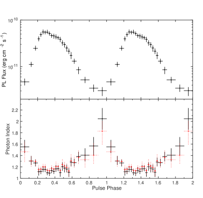
Figure 9.— Phase variation of the PL flux (upper panel) and the photon index (lower panel) for B1509. The black points are obtained with a simple PL fit and the red points are obtained with PL+BB fit. All uncertainties are at 90 % confidence level.

We therefore added a blackbody (BB) component to the off-pulse spectrum and tried fitting its temperature and normalization. We obtained $\Gamma=1.5^{+0.2}_{-0.3}$, $kT=0.17_{-0.05}^{+0.06}$ keV, and $\chi_{\nu}^{2}=0.94$, which significantly improves the fit with an $F$-test null hypothesis probability of $1.3\times 10^{-4}$. Assuming a distance of 5.2 kpc, the BB radius is $R_{\rm{BB}}=9_{-5}^{+38}$ km, not very well constrained albeit compatible with the canonical neutron star radius. We then fixed the normalization by assuming that the emission is from the entire surface of a neutron star with a radius of 13 km. The best-fit result yielded $\Gamma=1.6\pm 0.2$, $kT=0.147^{+0.007}_{-0.01}$ keV, and the absorbed 0.5–7 keV fluxes of $2.2^{+0.6}_{-0.5}\times 10^{-12}$ erg cm^-2 s^-1 and $8^{+20}_{-5}\times 10^{-14}$ erg cm^-2 s^-1 for the PL and BB components, respectively. We note that $\Gamma$ is flatter than that obtained by fitting a single PL because part of the soft X-ray emission is contributed by the BB component. The best-fit parameters are listed in Table 3. We also used the abundances by Anders & Grevesse (1989) with the absorption model phabs since the soft BB component could sensitively depend on the absorption model . The result is consistent with that obtained using tbnew. We also attempted to use the Cash statistics (Cash, 1979) to perform the same simultaneous fits without grouping the photons into energy bins. The result is fully consistent with that obtained from the $\chi^{2}$ statistics (see Table 3), and the likelihood ratio test suggested that adding a BB component can significantly improve the fit at a null hypothesis probability of $6\times 10^{-6}$.

Table 4Variation in Photon Index of B1509 Obtained with the PL and the PL+BB Fits to the Chandra Phase-resolved Spectrum.

Pulse Phase	$\Gamma$ (PL)	$\Gamma$ (PL+BB)
0.0–0.1	$1.55\pm 0.11$	$1.46\pm 0.18$
0.1–0.15	$1.30^{+0.09}_{-0.06}$	$1.30\pm 0.10$
0.15–0.2	$1.27_{-0.05}^{+0.06}$	$1.29_{-0.05}^{+0.08}$
0.2–0.225	$1.12\pm 0.06$	$1.15_{-0.07}^{+0.06}$
0.225–0.25	$1.12_{-0.04}^{+0.06}$	$1.16_{-0.05}^{+0.07}$
0.25–0.275	$1.15_{-0.04}^{+0.06}$	$1.20_{-0.05}^{+0.06}$
0.275–0.3	$1.15_{-0.04}^{+0.06}$	$1.20_{-0.05}^{+0.06}$
0.3–0.325	$1.10_{-0.04}^{+0.06}$	$1.14\pm 0.05$
0.325–0.35	$1.09_{-0.04}^{+0.05}$	$1.13_{-0.05}^{+0.07}$
0.35–0.375	$1.14_{-0.04}^{+0.06}$	$1.18\pm 0.06$
0.375–0.4	$1.12_{-0.04}^{+0.05}$	$1.16_{-0.05}^{+0.06}$
0.4–0.425	$1.17_{-0.05}^{+0.06}$	$1.20_{-0.09}^{+0.07}$
0.425–0.45	$1.17_{-0.04}^{+0.06}$	$1.20_{-0.05}^{+0.07}$
0.45–0.475	$1.10_{-0.07}^{+0.06}$	$1.13\pm 0.07$
0.475–0.5	$1.20\pm 0.07$	$1.24_{-0.09}^{+0.06}$
0.5–0.525	$1.18_{-0.07}^{+0.06}$	$1.20_{-0.09}^{+0.08}$
0.525–0.55	$1.16_{-0.05}^{+0.08}$	$1.19_{-0.07}^{+0.09}$
0.55–0.575	$1.11\pm 0.08$	$1.13_{-0.10}^{+0.09}$
0.575–0.6	$1.29_{-0.07}^{+0.08}$	$1.30_{-0.11}^{+0.09}$
0.6–0.65	$1.27\pm 0.06$	$1.28_{-0.11}^{+0.09}$
0.65–0.7	$1.38\pm 0.08$	$1.37\pm 0.11$
0.7–0.8	$1.41_{-0.10}^{+0.12}$	$1.32_{-0.11}^{+0.13}$
0.8–0.9	$1.57\pm 0.15$	$1.41_{-0.22}^{+0.14}$
0.9–1.0	$2.05\pm 0.19$	$1.82_{-0.18}^{+0.23}$
Pulsed	$1.18\pm 0.04$	$\cdots$
Off-pulse	$1.85\pm 0.15$	$1.5^{+0.3}_{-0.2}$
Phase-averaged	$1.18\pm 0.03$	$\cdots$
Tied Parameters and Statistics
Parameter	PL	PL+BB
$N_{\rm{H}}$ ($10^{22}$ cm-2)	$1.44\pm 0.04$	$1.55\pm 0.05$
$kT$ (keV)	$\cdots$	$0.142^{+0.007}_{-0.009}$
$\chi^{2}/dof$	2016.4/2145	1993.8/2144

Note. — The phase-averaged, pulsed, and off-pulse results are also listed for reference. We did not attempt to add the blackbody component to the phase-averaged spectrum because it is dominated by the pulsed emission that is well described by a power law.

We also tried using a more physical neutron star atmosphere model, nsa, to describe the soft component. However, the fitting is not significantly better than a simple BB and the best-fit surface temperature is similar. Finally, as a consistency check, we convolved the best-fit BB+PL model with the HRC response, and this predicts 386 counts from the pulsar, which is fully consistent with the observed 390 counts. Note that the background is negligible at a level of $\lesssim 10$ photons.

3.4.4 Phase Variation of the Spectrum

To investigate the phase variation of the spectrum, we divided the X-ray photons into 24 phase bins. The bin length for the low-intensity (phase 0.7–1.1), the transition (phase 0.1–0.2 and 0.6–0.7), and the high-intensity (phase 0.2–0.6) states are 0.1, 0.05, and 0.025, respectively. We first fit all the 24 spectra simultaneously with a simple PL model and a single $N_{\rm{H}}$ value. The fit is acceptable with an $N_{\rm{H}}=(1.44\pm 0.04)\times 10^{22}$ cm^-2. The variation of the PL flux and the best-fit photon index with phase is shown in Figure 9. $\Gamma$ stays at $\approx 1.15$ between phase 0.2–0.6 and increases when the flux decreases after phase $\sim 0.6$, until it reaches a maximum value of $2.0\pm 0.2$ in the faintest phase bin. We did not find significant spectral variation around phase 0.4, indicating that the bump structure in the profile (see Section 3.3) is possibly a statistical fluctuation.

Similar to the analysis in Section 3.4.3, we then added a BB component across all phases and set the BB temperature and radius as free parameters. The fit was significantly improved with an $F$-test null hypothesis probability of $4.6\times 10^{-6}$, and the BB temperature is $kT=0.13\pm 0.03$ keV. However, the BB radius is $18_{-10}^{+70}$ km, not well constrained although consistent with that in the off-pulse fit. Therefore, we fixed the BB normalization by assuming that BB emission arises from the entire surface of a neutron star. The fits yielded a consistent $N_{\rm{H}}=(1.55\pm 0.05)\times 10^{22}$ cm^-2, and the BB temperature was determined as $kT=0.142^{+0.007}_{-0.009}$ keV. After adding a BB component, the photon indices are systematically lower than those obtained from a single PL fit when the flux is low. The photon index again shows variability, albeit slightly less significant. The results are listed in Table 4, together with the parameters for the pulsed, off-pulse, and phase-averaged spectra.

4. Discussion

4.1. Thermal Emission

Our spectral analysis shows evidence of thermal emission from B1509, with a BB temperature of $\sim$0.14 keV. To compare the surface temperature with other high magnetic field RPPs, typical RPPs, and magnetars, we plotted their thermal luminosities and compared with theoretical models in Figure 10. Neutron stars are born as hot objects and then cool down rapidly by neutrino emission through the Urca process in the core, although different equations of state may result in a variety of cooling timescales (see, e.g., Nomoto & Tsuruta, 1987; Lattimer et al., 1991; Akmal et al., 1998). In general, the surface temperature of a neutron star drops to $T\lesssim 10^{6}$ K after $\sim 10^{3}$ yr. The observational results of typical RPPs (see, e.g., Shternin et al., 2011; Weisskopf et al., 2011) agree with the theoretical predictions, and they occupy the lower part of Figure 10.

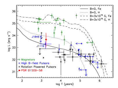
Figure 10.— Theoretical cooling curves adopted from Viganò et al. (2013) for a 1.4M_⊙ neutron star with zero magnetic field and an Fe envelope (solid line), zero magnetic field and an H envelope (dotted line), strong magnetic field and an Fe envelope (dashed line), and strong magnetic field and an H envelope (dash-dotted line). The data points show the observed thermal luminosities of magnetars (green diamond), high magnetic field RPPs (blue squares), typical RPPs (black crosses), and B1509 (red filled circle). The magnetar values are adopted from Viganò et al. (2013), with updated ages from the McGill Magnetar Catalog (Olausen & Kaspi, 2014). The RPP measurements and upper limits are from Shternin et al. (2011), Weisskopf et al. (2011), and Viganò et al. (2013). The high magnetic field RPPs are from Gonzalez et al. (2004), Kaspi & McLaughlin (2005), McLaughlin et al. (2007), Safi-Harb & Kumar (2008), Kaplan et al. (2009), Zhu et al. (2009), Livingstone et al. (2011), Ng et al. (2012), Keane et al. (2013), and Olausen et al. (2013).

The discovery of magnetars breaks the expectation owing to their high surface temperature of $T>5\times 10^{6}$ K and high thermal luminosities $L=10^{34}-10^{36}$ erg s^-1. They are thought to be powered by the dissipation of a strong magnetic field (Thompson & Duncan, 1995). A theory that unifies the magnetars and RPPs is the magneto-thermal evolution model (Pons et al., 2009; Perna & Pons, 2011; Viganò et al., 2013). In this model, the decay of the crustal magnetic field causes the magnetar activities and the high surface temperature, and it is dominated by the Ohmic dissipation and the Hall drift (Glampedakis et al., 2011). The time evolution of the $B$-field can be described by

$$\begin{split}\frac{\partial\mathbf{B}}{\partial t}=&-\nabla\times\left\{\frac{c^{2}}{4\pi\sigma}\nabla\times\left(\rm{e}^{\nu}\mathbf{B}\right)\right.\\ &\left.+\frac{c}{4\pi en_{e}}\left[\nabla\times\left(\rm{e}^{\nu}\mathbf{B}\right)\right]\times\mathbf{B}\right\},\end{split}$$ (4)

where $\mathbf{B}$ is the surface field measured by the observer at rest, $\sigma$ is the conductivity, $\rm{e}^{\nu}$ is the lapse function that accounts for the relativistic redshift, $e$ is the elementary charge, and $n_{e}$ is the electron number density. A stronger initial field indicates a higher energy dissipation and results in a higher surface luminosity. We adopted the theoretical cooling curves produced by Viganò et al. (2013), which took all these effects into account. We plotted two cases of the initial magnetic field strengths of 0 and $3\times 10^{15}$ G. Below ages of $\sim 10^{4}$ yr, magnetars, high magnetic field RPPs, and typical RPPs occupy different regions in Figure 10. Typical RPPs are consistent with the evolutionary tracks of $B=0$ with luminosities lower than $\sim 10^{33}$ erg s^-1. Magnetars, which have much higher thermal luminosities at $10^{34}$–$10^{36}$ erg s^-1, are well described by the tracks of high $B$-fields. The thermal luminosity of B1509 is comparable with other high magnetic field RPPs, e.g., PSR J1119$-$6127 with $L\approx 2\times 10^{33}$ erg s^-1 (Ng et al., 2012), which are in between the typical RPPs and magnetars. This result fits the magneto-thermal evolution model well.

Finally, we note that the return current in the magnetosphere could also heat the neutron star surface (Zhang & Cheng, 1997, 2000). The hard X-rays from the polar cap are reflected back to the entire stellar surface and cause a temperature of

$$T_{s}\sim 3.8\times 10^{5}f_{0}^{1/4}P^{-5/12}B_{12}^{1/4}\rm{\,K~{},}$$ (5)

where $f_{0}\sim 0.12$ for B1509 is the average size of the outer gap, $P$ is the spin period, and $B_{12}$ is the surface magnetic field in a unit of $10^{12}$ G (Zhang & Cheng, 2000). In the case of B1509, this effect gives a surface temperature of only $\sim 0.08$ keV, contributing a thermal luminosity lower than 9 % of the measured value. Hence, it is negligible in our discussion.

In the magneto-thermal theory above, the luminosity of a neutron star is related to the magnetic field strength, which consists of the poloidal and the toroidal components. However, only the former can be inferred from the spin down, and the latter is not directly observable. Our detection of thermal emission from B1509 completes the sample of young, high magnetic field RPPs with age $<2000$ years. It has a similar thermal luminosity and age as other sources (namely PSRs J1846$-$0258 and J1119$-$6127) in the group. We therefore speculate that B1509 has a comparable total $B$-field strength, although its dipole field is slightly weaker. High magnetic field RPPs are expected to show magnetar-like bursts as magnetars. This idea was first suggested by Kaspi & McLaughlin (2005) and then observed in PSRs J1846$-$0258 and J1119$-$6127. By estimating the frequency of starquakes, Perna & Pons (2011) suggested that all types of pulsars could show magnetar-like activities, although the occurrence rate is low for lower field and aged objects. If this is true, we may expect to find magnetar-like activities in B1509 in the sam way as in the other two high magnetic field RPPs since their ages and total $B$-fields are similar.

4.2. Nonthermal Emission

Another intriguing feature of B1509 is that the X-ray spectrum becomes softer when the flux decreases from the pulse peak. Similar behavior has been found in other young pulsars, including the Crab (Weisskopf et al., 2011; Ge et al., 2012), PSR J1930+1852 (Lu et al., 2007), and PSR B0540$-$69 (Hirayama et al., 2002; Ge et al., 2012). Of these, the Crab pulsar is the best-studied source. Its profile shows a double-peaked feature from radio to $\gamma$-ray bands (Toor & Seward, 1977; Pravdo & Serlemitsos, 1981). The variation in photon index between the two peaks has been interpreted by both the outer-gap model (Zhang & Cheng, 2002) and a phenomenological two-component model (Massaro et al., 2000). A recent Chandra observation discovered a large photon index of the Crab’s off-pulse emission (Weisskopf et al., 2011), which cannot be explained by any previous models.

Unlike the Crab, the other pulsars show single-peaked X-ray profiles, and the profiles of both PSRs B1509$-$58 and B0540$-$69 can be fit with two Gaussians. Taking this feature into account, their X-ray spectra are hardest between the two Gaussian peaks (Ge et al., 2012), which qualitatively agrees with the behavior of the Crab if the two Gaussians are considered as the two peaks. Moreover, these two pulsars exhibit significant softening of the off-pulse emission similar to that of the Crab pulsar (Hirayama et al., 2002). For PSR J1930+1852, this was only inferred from the HR (Lu et al., 2007) and could possibly be due to contamination by the BB emission. Therefore, further deep observation is needed to investigate its spectral behavior.

We can qualitatively explain the phase variation of the photon index of B1509 using the outer-gap model. In this model, the discharged pairs in the pulsar magnetosphere produce gamma-rays, which subsequently create secondary pairs that give synchrotron emission in the X-ray band. The viewing angle of B1509 only allows us to detect the synchrotron radiation of the pairs created by the incoming gamma-rays (Wang et al., 2013). The created pairs are quickly cooled down to the lowest Landau level via synchrotron emission, with the photon energy given by

$$E_{syn}\sim 3h\gamma^{2}B/4\pi m_{e}c\sim 170{\rm MeV}(\gamma/10^{3})^{2}(B/10^{10}{\rm G})\rm{,}$$ (6)

with $\gamma$ being the Lorentz factor of the pairs and $B$ being the magnetic field strength at the pair-creation site. The spectrum has a high-energy cutoff of $E_{max}\sim 170{\rm\,MeV}(B/10^{10}{\rm\,G})$ owing to the maximum energy of the created pair with $\gamma\sim 1000$. This is much higher than the Chandra energy range. In addition, a low-energy turnover is present due to the cooled-down pair with a final Lorentz factor of $\gamma\sim 1$ as $E_{min}\sim 170{\rm\,eV}(B/10^{10}{\rm\,G})$. Below this, the spectrum is described by the low-energy tail of the synchrotron radiation, which has an asymptotic form of a PL with $\Gamma\sim 2/3$ (Rybicki & Lightman, 1986). Between these two critical energies, the spectrum has $\Gamma\sim 1.5$ determined by the energy distribution of the pairs. Hence, the photon index in the X-ray band is controlled by the value of $E_{min}$, which is proportional to the magnetic field strength.

According to this model, the pair-creation process of B1509 has two origins. The first origin is magnetic-photon pair creation, which occurs near the magnetic pole because a stronger magnetic field is needed, thus the synchrotron emission is observed at a narrower viewing angle. As the $B$-field is strong near the pole, $E_{min}$ is lower and hence this emission has a flatter spectrum. The pulsed X-ray emission of B1509 is dominated by this process. The other process is photon-photon pair creation, which is distributed more isotropically in the entire magnetosphere, and $E_{min}$ is located in optical/UV bands owing to the lower magnetic field. The off-pulse emission is dominated by this process, and the X-ray emission is much softer than the pulsed one. Consequently, the variation in spectral index can be qualitatively explained by the various amounts of contribution from these emission processes across the rotational phase.

5. Summary

We performed a detailed timing and phase-resolved spectral analysis of the high magnetic field RPP B1509 using high-resolution Chandra observations. The pulse profile can be fit by two Gaussian components, and the pulsed fraction is energy dependent. The 0.5–7 keV pulsed spectrum is well described by a PL with a photon index of 1.18, lower than the indices at higher energy bands. This result is consistent with the broadband curved logpar spectrum. The off-pulse spectrum can be fit by a PL plus BB model. The photon index is significantly higher, and the BB has a temperature of $\sim$0.14 keV. The thermal luminosity of B1509 we obtained is comparable with the luminosities of two other young high magnetic field RPPs, J1846$-$0258 and J1119$-$6127, and it is brighter than the luminosities of normal RPPs. This result supports the magneto-thermal evolution model, indicating that these sources belong to the transition class of neutron stars between magnetars and RPPs and could show magnetar-like activities. We also found that the nonthermal emission in the off-pulse phase has a much softer spectrum. This behavior is similar to other young and energetic pulsars, including the Crab, PSRs B0540$-$69 and J1930+1852. We interpreted it qualitatively using the outer-gap model, in which the pulsed emission of B1509 is dominated by the magnetic-photon pair creation near the stellar surface, while the off-pulse nonthermal emission is dominated by the isotropic photon-photon pair creation.

References

- Akmal et al. (1998) Akmal, A., Pandharipande, V. R., & Ravenhall, D. G. 1998, PhRvC, 58, 1804
- Anders & Grevesse (1989) Anders, E., & Grevesse, N. 1989, GeCoA, 53, 197
- Archibald et al. (2016) Archibald, R. F., Kaspi, V. M., Tendulkar, S. P., & Scholz, P. 2016, ApJ, 829, L21
- Beloborodov & Li (2016) Beloborodov, A. M., & Li, X. 2016, ApJ, 833, 261
- Cash (1979) Cash, W. 1979, ApJ, 228, 939
- Chen et al. (2016) Chen, G., An, H., Kaspi, V. M., et al. 2016, ApJ, 817, 93
- Cusumano et al. (2001) Cusumano, G., Mineo, T., Massaro, E., et al. 2001, A&A, 375, 397
- de Jager et al. (1989) de Jager, O. C., Raubenheimer, B. C., & Swanepoel, J. W. H. 1989, A&A, 221, 180
- DeLaney et al. (2006) DeLaney, T., Gaensler, B. M., Arons, J., & Pivovaroff, M. J. 2006, ApJ, 640, 929
- Dib et al. (2009) Dib, R., Kaspi, V. M., & Gavriil, F. P. 2009, ApJ, 702, 614
- Freeman et al. (2001) Freeman, P., Doe, S., & Siemiginowska, A. 2001, Proc. SPIE, 4477, 76
- Fruscione et al. (2006) Fruscione, A., McDowell, J. C., Allen, G. E., et al. 2006, Proc. SPIE, 6270, 62701V
- Gaensler et al. (2002) Gaensler, B. M., Arons, J., Kaspi, V. M., et al. 2002, ApJ, 569, 878
- Gaensler et al. (1999) Gaensler, B. M., Brazier, K. T. S., Manchester, R. N., Johnston, S., & Green, A. J. 1999, MNRAS, 305, 724
- Gavriil et al. (2008) Gavriil, F. P., Gonzalez, M. E., Gotthelf, E. V., et al. 2008, Science, 319, 1802
- Ge et al. (2012) Ge, M. Y., Lu, F. J., Qu, J. L., et al. 2012, ApJS, 199, 32
- Glampedakis et al. (2011) Glampedakis, K., Jones, D. I., & Samuelsson, L. 2011, MNRAS, 413, 2021
- Gonzalez et al. (2004) Gonzalez, M. E., Kaspi, V. M., Lyne, A. G., & Pivovaroff, M. J. 2004, ApJ, 610, L37
- Göğüş et al. (2016) Göğüş, E., Lin, L., Kaneko, Y., et al. 2016, ApJ, 829, L25
- Greiveldinger et al. (1995) Greiveldinger, C., Caucino, S., Massaglia, S., Oegelman, H., & Trussoni, E. 1995, ApJ, 454, 855
- Hirayama et al. (2002) Hirayama, M., Nagase, F., Endo, T., Kawai, N., & Itoh, M. 2002, MNRAS, 333, 603
- Hobbs et al. (2004) Hobbs, G., Lyne, A. G., Kramer, M., Martin, C. E., & Jordan, C. 2004, MNRAS, 353, 1311
- Kaplan et al. (2009) Kaplan, D. L., Esposito, P., Chatterjee, S., et al. 2009, MNRAS, 400, 1445
- Kaspi et al. (1994) Kaspi, V. M., Manchester, R. N., Siegman, B., Johnston, S., & Lyne, A. G. 1994, ApJ, 422, L83
- Kaspi & McLaughlin (2005) Kaspi, V. M., & McLaughlin, M. A. 2005, ApJ, 618, L41
- Kawai et al. (1991) Kawai, N., Okayasu, R., Brinkmann, W., et al. 1991, ApJ, 383, L65
- Keane et al. (2013) Keane, E. F., McLaughlin, M. A., Kramer, M., et al. 2013, ApJ, 764, 180
- Kuiper & Hermsen (2015) Kuiper, L., & Hermsen, W. 2015, MNRAS, 449, 3827
- Kuiper et al. (1999) Kuiper, L., Hermsen, W., Krijger, J. M., et al. 1999, A&A, 351, 119
- Lattimer et al. (1991) Lattimer, J. M., Prakash, M., Pethick, C. J., & Haensel, P. 1991, PhRvL, 66, 2701
- Livingstone et al. (2011) Livingstone, M. A., Ng, C.-Y., Kaspi, V. M., Gavriil, F. P., & Gotthelf, E. V. 2011, ApJ, 730, 66
- Lu et al. (2007) Lu, F., Wang, Q. D., Gotthelf, E. V., & Qu, J. 2007, ApJ, 663, 315
- Manchester et al. (1982) Manchester, R. N., Tuohy, I. R., & Damico, N. 1982, ApJ, 262, L31
- Marsden et al. (1997) Marsden, D., Blanco, P. R., Gruber, D. E., et al. 1997, ApJ, 491, L39
- Massaro et al. (2000) Massaro, E., Cusumano, G., Litterio, M., & Mineo, T. 2000, A&A, 361, 695
- McLaughlin et al. (2007) McLaughlin, M. A., Rea, N., Gaensler, B. M., et al. 2007, ApJ, 670, 1307
- Mereghetti (2008) Mereghetti, S. 2008, A&ARv, 15, 225
- Mereghetti et al. (2015) Mereghetti, S., Pons, J. A., & Melatos, A. 2015, Space Sci. Rev., 191, 315
- Mills et al. (1960) Mills, B. Y., Slee, O. B., & Hill, E. R. 1960, AuJPh, 13, 676
- Ng et al. (2012) Ng, C.-Y., Kaspi, V. M., Ho, W. C. G., et al. 2012, ApJ, 761, 65
- Ng et al. (2008) Ng, C.-Y., Slane, P. O., Gaensler, B. M., & Hughes, J. P. 2008, ApJ, 686, 508
- Nomoto & Tsuruta (1987) Nomoto, K., & Tsuruta, S. 1987, ApJ, 312, 711
- Olausen & Kaspi (2014) Olausen, S. A., & Kaspi, V. M. 2014, ApJS, 212, 6
- Olausen et al. (2013) Olausen, S. A., Zhu, W. W., Vogel, J. K., et al. 2013, ApJ, 764, 1
- Perna & Pons (2011) Perna, R., & Pons, J. A. 2011, ApJ, 727, L51
- Pons & Geppert (2007) Pons, J. A., & Geppert, U. 2007, A&A, 470, 303
- Pons et al. (2009) Pons, J. A., Miralles, J. A., & Geppert, U. 2009, A&A, 496, 207
- Pravdo & Serlemitsos (1981) Pravdo, S. H., & Serlemitsos, P. J. 1981, ApJ, 246, 484
- Rea et al. (2010) Rea, N., Esposito, P., Turolla, R., et al. 2010, Science, 330, 944
- Rea et al. (2013) Rea, N., Israel, G. L., Pons, J. A., et al. 2013, ApJ, 770, 65
- Rots et al. (1998) Rots, A. H., Jahoda, K., Macomb, D. J., et al. 1998, ApJ, 501, 749
- Rybicki & Lightman (1986) Rybicki, G. B., & Lightman, A. P. 1986, Radiative Processes in Astrophysics (Hoboken, NJ: Wiley-VCH)
- Safi-Harb & Kumar (2008) Safi-Harb, S., & Kumar, H. S. 2008, ApJ, 684, 532
- Schöck et al. (2010) Schöck, F. M., Büsching, I., de Jager, O. C., Eger, P., & Vorster, M. J. 2010, A&A, 515, A109
- Scholz et al. (2012) Scholz, P., Ng, C.-Y., Livingstone, M. A., et al. 2012, ApJ, 761, 66
- Seward & Harnden (1982) Seward, F. D., & Harnden, Jr., F. R. 1982, ApJ, 256, L45
- Shternin et al. (2011) Shternin, P. S., Yakovlev, D. G., Heinke, C. O., Ho, W. C. G., & Patnaude, D. J. 2011, MNRAS, 412, L108
- Thompson & Duncan (1995) Thompson, C., & Duncan, R. C. 1995, MNRAS, 275, 255
- Thompson & Duncan (1996) —. 1996, ApJ, 473, 322
- Toor & Seward (1977) Toor, A., & Seward, F. D. 1977, ApJ, 216, 560
- Turolla et al. (2015) Turolla, R., Zane, S., & Watts, A. L. 2015, RPPh, 78, 116901
- Viganò et al. (2013) Viganò, D., Rea, N., Pons, J. A., et al. 2013, MNRAS, 434, 123
- Wang et al. (2013) Wang, Y., Takata, J., & Cheng, K. S. 2013, ApJ, 764, 51
- Weisskopf et al. (2011) Weisskopf, M. C., Tennant, A. F., Yakovlev, D. G., et al. 2011, ApJ, 743, 139
- Weisskopf et al. (1983) Weisskopf, M. C., Elsner, R. F., Darbro, W., et al. 1983, ApJ, 267, 711
- Weltevrede et al. (2010) Weltevrede, P., Johnston, S., Manchester, R. N., et al. 2010, PASA, 27, 64
- Wilms et al. (2000) Wilms, J., Allen, A., & McCray, R. 2000, ApJ, 542, 914
- Yatsu et al. (2009) Yatsu, Y., Kawai, N., Shibata, S., & Brinkmann, W. 2009, PASJ, 61, 129
- Zhang & Cheng (1997) Zhang, L., & Cheng, K. S. 1997, ApJ, 487, 370
- Zhang & Cheng (2000) —. 2000, A&A, 363, 575
- Zhang & Cheng (2002) —. 2002, ApJ, 569, 872
- Zhu et al. (2009) Zhu, W., Kaspi, V. M., Gonzalez, M. E., & Lyne, A. G. 2009, ApJ, 704, 1321