On Kernelized Multi-armed Bandits

Abstract

We consider the stochastic bandit problem with a continuous set of arms, with the expected reward function over the arms assumed to be fixed but unknown. We provide two new Gaussian process-based algorithms for continuous bandit optimization – Improved GP-UCB (IGP-UCB) and GP-Thomson sampling (GP-TS), and derive corresponding regret bounds. Specifically, the bounds hold when the expected reward function belongs to the reproducing kernel Hilbert space (RKHS) that naturally corresponds to a Gaussian process kernel used as input by the algorithms. Along the way, we derive a new self-normalized concentration inequality for vector-valued martingales of arbitrary, possibly infinite, dimension. Finally, experimental evaluation and comparisons to existing algorithms on synthetic and real-world environments are carried out that highlight the favorable gains of the proposed strategies in many cases.

1 Introduction

Optimization over large domains under uncertainty is an important subproblem arising in a variety of sequential decision making problems, such as dynamic pricing in economics (Besbes and Zeevi, 2009), reinforcement learning with continuous state/action spaces (Kaelbling et al., 1996; Smart and Kaelbling, 2000), and power control in wireless communication (Chiang et al., 2008). A typical feature of such problems is a large, or potentially infinite, domain of decision points or covariates (prices, actions, transmit powers), together with only partial and noisy observability of the associated outcomes (demand, state/reward, communication rate); reward/loss information is revealed only for decisions that are chosen. This often makes it hard to balance exploration and exploitation, as available knowledge must be transferred efficiently from a finite set of observations so far to estimates of the values of infinitely many decisions. A classic case in point is that of the canonical stochastic MAB with finitely many arms, where the effort to optimize scales with the total number of arms or decisions; the effect of this is catastrophic for large or infinite arm sets.

With suitable structure in the values or rewards of arms, however, the challenge of sequential optimization can be efficiently addressed. Parametric bandits, especially linearly parameterized bandits (Rusmevichientong and Tsitsiklis, 2010), represent a well-studied class of structured decision making settings. Here, every arm corresponds to a known, finite dimensional vector (its feature vector), and its expected reward is assumed to be an unknown linear function of its feature vector. This allows for a large, or even infinite, set of arms all lying in space of finite dimension, say $d$, and a rich line of work gives algorithms that attain sublinear regret with a polynomial dependence on the dimension, e.g., Confidence Ball (Dani et al., 2008), OFUL (Abbasi-Yadkori et al., 2011) (a strengthening of Confidence Ball) and Thompson sampling for linear bandits (Agrawal and Goyal, 2013) The insight here is that even though the number of arms can be large, the number of unknown parameters (or degrees of freedom) in the problem is really only $d$, which makes it possible to learn about the values of many other arms by playing a single arm.

A different approach to modelling bandit problems with a continuum of arms is via the framework of Gaussian processes (GPs) (Rasmussen and Williams, 2006). GPs are a flexible class of nonparametric models for expressing uncertainty over functions on rather general domain sets, which generalize multivariate Gaussian random vectors. GPs allow tractable regression for estimating an unknown function given a set of (noisy) measurements of its values at chosen domain points. The fact that GPs, being distributions on functions, can also help quantify function uncertainty makes it attractive for basing decision making strategies on them. This has been exploited to great advantage to build nonparametric bandit algorithms, such as GP-UCB (Srinivas et al., 2009), GP-EI and GP-PI (Hoffman et al., 2011). In fact, GP models for bandit optimization, in terms of their kernel maps, can be viewed as the parametric linear bandit paradigm pushed to the extreme, where each feature vector associated to an arm can have infinite dimension .

Against this backdrop, our work revisits the problem of bandit optimization with stochastic rewards. Specifically, we consider stochastic multiarmed bandit (MAB) problems with a continuous arm set, and whose (unknown) expected reward function is assumed to lie in a reproducing kernel Hilbert space (RKHS), with bounded RKHS norm – this effectively enforces smoothness on the function. We make the following contributions-

• We design a new algorithm – Improved Gaussian Process-Upper Confidence Bound (IGP-UCB) – for stochastic bandit optimization. The algorithm can be viewed as a variant of GP-UCB (Srinivas et al., 2009), but uses a significantly reduced confidence interval width resulting in an order-wise improvement in regret compared to GP-UCB. IGP-UCB also shows a markedly improved numerical performance over GP-UCB.

• We develop a nonparametric version of Thompson sampling, called Gaussian Process Thompson sampling (GP-TS), and show that enjoys a regret bound of $\tilde{O}\left(\gamma_{T}\sqrt{dT}\right)$. Here, $T$ is the total time horizon and $\gamma_{T}$ is a quantity depending on the RKHS containing the reward function. This is, to our knowledge, the first known regret bound for Thompson sampling in the agnostic setup with nonparametric structure.

• We prove a new self-normalized concentration inequality for infinite-dimensional vector-valued martingales, which is not only key to the design and analysis of the IGP-UCB and GP-TS algorithms, but also potentially of independent interest. The inequality generalizes a corresponding self-normalized bound for martingales in finite dimension proven by Abbasi-Yadkori et al. (2011).

• Empirical comparisons of the algorithms developed above, with other GP-based algorithms, are presented, over both synthetic and real-world setups, demonstrating performance improvements of the proposed algorithms, as well as their performance under misspecification.

2 Problem Statement

We consider the problem of sequentially maximizing a fixed but unknown reward function $f:D\rightarrow\mathbb{R}$ over a (potentially infinite) set of decisions $D\subset\mathbb{R}^{d}$, also called actions or arms. An algorithm for this problem chooses, at each round $t$, an action $x_{t}\in D$, and subsequently observes a reward $y_{t}=f(x_{t})+\varepsilon_{t}$, which is a noisy version of the function value at $x_{t}$. The action $x_{t}$ is chosen causally depending upon the arms played and rewards obtained upto round $t-1$, denoted by the history $\mathcal{H}_{t-1}=\{(x_{s},y_{s}):s=1,\ldots,t-1\}$. We assume that the noise sequence $\{\varepsilon_{t}\}_{t=1}^{\infty}$ is conditionally $R$-sub-Gaussian for a fixed constant $R\geq 0$, i.e.,

$$\forall t\geq 0,\;\;\forall\lambda\in\mathbb{R},\;\;\mathbb{E}\left[{e^{\lambda\varepsilon_{t}}\;\big{|}\;\mathcal{F}_{t-1}}\right]\leq\exp\left(\frac{\lambda^{2}R^{2}}{2}\right),$$ (1)

where $\mathcal{F}_{t-1}$ is the $\sigma$-algebra generated by the random variables $\{x_{s},\varepsilon_{s}\}_{s=1}^{t-1}$ and $x_{t}$.This is a mild assumption on the noise (it holds, for instance, for distributions bounded in $[-R,R]$) and is standard in the bandit literature (Abbasi-Yadkori et al., 2011; Agrawal and Goyal, 2013).

Regret. The goal of an algorithm is to maximize its cumulative reward or alternatively minimize its cumulative regret – the loss incurred due to not knowing $f$’s maximum point beforehand. Let $x^{\star}\in\mathop{\mathrm{argmax}}_{x\in D}f(x)$ be a maximum point of $f$ (assuming the maximum is attained). The instantaneous regret incurred at time $t$ is $r_{t}=f(x^{\star})-f(x_{t})$, and the cumulative regret in a time horizon $T$ (not necessarily known a priori) is defined to be $R_{T}=\sum_{t=1}^{T}r_{t}$. A sub-linear growth of $R_{T}$ in $T$ signifies that $R_{T}/T\rightarrow 0$ as $T\rightarrow\infty$, or vanishing per-round regret.

Regularity Assumptions. Attaining sub-linear regret is impossible in general for arbitrary reward functions $f$ and domains $D$, and thus some regularity assumptions are in order. In what follows, we assume that $D$ is compact. The smoothness assumption we make on the reward function $f$ is motivated by Gaussian processes and their associated reproducing kernel Hilbert spaces (RKHSs, see Schölkopf and Smola (2002)). Specifically, we assume that $f$ has small norm in the RKHS of functions $D\to\mathbb{R}$, with positive semi-definite kernel function $k:D\times D\to\mathbb{R}$. This RKHS, denoted by $H_{k}(D)$, is completely specified by its kernel function $k(\cdot,\cdot)$ and vice-versa, with an inner product $\langle\cdot,\cdot\rangle_{k}$ obeying the reproducing property: $f(x)=\langle f,k(x,\cdot)\rangle_{k}$ for all $f\in H_{k}(D)$. In other words, the kernel plays the role of delta functions to represent the evaluation map at each point $x\in D$ via the RKHS inner product. The RKHS norm $\left\lVert f\right\rVert_{k}=\sqrt{\langle f,f\rangle}_{k}$ is a measure of the smoothness of $f$, with respect to the kernel function $k$, and satisfies: $f\in H_{k}(D)$ if and only if $\left\lVert f\right\rVert_{k}<\infty$.

We assume a known bound on the RKHS norm of the unknown target function: $\left\lVert f\right\rVert_{k}\leq B$. Moreover, we assume bounded variance by restricting $k(x,x)\leq 1$, for all $x\in D$. Two common kernels that satisfy bounded variance property are Squared Exponential and Mat$\acute{e}$rn, defined as

$$k_{SE}(x,x^{\prime}) = \exp\Big{(}-s^{2}/2l^{2}\Big{)},$$

$$k_{Mat\acute{e}rn}(x,x^{\prime}) = \frac{2^{1-\nu}}{\Gamma(\nu)}\Big{(}\frac{s\sqrt{2\nu}}{l}\Big{)}^{\nu}B_{\nu}\Big{(}\frac{s\sqrt{2\nu}}{l}\Big{)},$$

where $l>0$ and $\nu>0$ are hyperparameters, $s=\left\lVert x-x^{\prime}\right\rVert_{2}$ encodes the similarity between two points $x,x^{\prime}\in D$, and $B_{\nu}(\cdot)$ is the modified Bessel function. Generally the bounded variance property holds for any stationary kernel, i.e. kernels for which $k(x,x^{\prime})=k(x-x^{\prime})$ for all $x,x^{\prime}\in\mathbb{R}^{d}$. These assumptions are required to make the regret bounds scale-free and are standard in the literature (Agrawal and Goyal, 2013). Instead if $k(x,x)\leq c$ or $\left\lVert f\right\rVert_{k}\leq cB$, then our regret bounds would increase by a factor of $c$.

3 Algorithms

Design philosophy. Both the algorithms we propose use Gaussian likelihood models for observations, and Gaussian process (GP) priors for uncertainty over reward functions. A Gaussian process over $D$, denoted by $GP_{D}(\mu(\cdot),k(\cdot,\cdot))$, is a collection of random variables $(f(x))_{x\in D}$, one for each $x\in D$, such that every finite sub-collection of random variables $(f(x_{i}))_{i=1}^{m}$ is jointly Gaussian with mean $\mathbb{E}\left[{f(x_{i})}\right]=\mu(x_{i})$ and covariance $\mathbb{E}\left[{(f(x_{i})-\mu(x_{i}))(f(x_{j})-\mu(x_{j}))}\right]=k(x_{i},x_{j})$, $1\leq i,j\leq m$, $m\in\mathbb{N}$. The algorithms use $GP_{D}(0,v^{2}k(\cdot,\cdot))$, $v>0$, as an initial prior distribution for the unknown reward function $f$ over $D$, where $k(\cdot,\cdot)$ is the kernel function associated with the RKHS $H_{k}(D)$ in which $f$ is assumed to have ‘small’ norm at most $B$. The algorithms also assume that the noise variables $\varepsilon_{t}=y_{t}-f(x_{t})$ are drawn independently, across $t$, from $\mathcal{N}(0,\lambda v^{2})$, with $\lambda\geq 0$. Thus, the prior distribution for each $f(x)$, is assumed to be $\mathcal{N}(0,v^{2}k(x,x))$, $x\in D$. Moreover, given a set of sampling points $A_{t}=(x_{1},\ldots,x_{t})$ within $D$, it follows under the assumption that the corresponding vector of observed rewards $y_{1:t}=[y_{1},\ldots,y_{t}]^{T}$ has the multivariate Gaussian distribution $\mathcal{N}(0,v^{2}(K_{t}+\lambda I))$, where $K_{t}=[k(x,x^{\prime})]_{x,x^{\prime}\in A_{t}}$ is the kernel matrix at time $t$. Then, by the properties of GPs, we have that $y_{1:t}$ and $f(x)$ are jointly Gaussian given $A_{t}$:

$$\begin{bmatrix}f(x)\\ y_{1:t}\end{bmatrix}\sim\mathcal{N}\left(0,\begin{bmatrix}v^{2}k(x,x)&v^{2}k_{t}(x)^{T}\\ v^{2}k_{t}(x)&v^{2}(K_{t}+\lambda I)\end{bmatrix}\right),$$

where $k_{t}(x)=[k(x_{1},x),\ldots,k(x_{t},x)]^{T}$. Therefore conditioned on the history $\mathcal{H}_{t}$, the posterior distribution over $f$ is $GP_{D}(\mu_{t}(\cdot),v^{2}k_{t}(\cdot,\cdot))$, where

$$\mu_{t}(x) = k_{t}(x)^{T}(K_{t}+\lambda I)^{-1}y_{1:t},$$ (2)

$$k_{t}(x,x^{\prime}) = k(x,x^{\prime})-k_{t}(x)^{T}(K_{t}+\lambda I)^{-1}k_{t}(x^{\prime}),$$ (3)

$$\sigma_{t}^{2}(x) = k_{t}(x,x).$$ (4)

Thus for every $x\in D$, the posterior distribution of $f(x)$, given $\mathcal{H}_{t}$, is $\mathcal{N}(\mu_{t}(x),v^{2}\sigma_{t}^{2}(x))$.

Remark. Note that the GP prior and Gaussian likelihood model described above is only an aid to algorithm design, and has nothing to do with the actual reward distribution or noise model as in the problem statement (Section 2). The reward function $f$ is a fixed, unknown, member of the RKHS $H_{k}(D)$, and the true sequence of noise variables $\varepsilon_{t}$ is allowed to be a conditionally $R$-sub-Gaussian martingale difference sequence (Equation 1). In general, thus, this represents a misspecified prior and noise model, also termed the agnostic setting by Srinivas et al. (2009).

The proposed algorithms, to follow, assume the knowledge of only the sub-Gaussianity parameter $R$, kernel function $k$ and upper bound $B$ on the RKHS norm of $f$. Note that $v,\lambda$ are free parameters (possibly time-dependent) that can be set specific to the algorithm.

3.1 Improved GP-UCB (IGP-UCB) Algorithm

We introduce the IGP-UCB algorithm (Algorithm 1), that uses a combination of the current posterior mean $\mu_{t-1}(x)$ and standard deviation $v\sigma_{t-1}(x)$ to (a) construct an upper confidence bound (UCB) envelope for the actual function $f$ over $D$, and (b) choose an action to maximize it. Specifically it chooses, at each round $t$, the action

$$x_{t}=\mathop{\mathrm{argmax}}_{x\in D}\mu_{t-1}(x)+\beta_{t}\sigma_{t-1}(x),$$ (5)

with the scale parameter $v$ set to be $1$. Such a rule trades off exploration (picking points with high uncertainty $\sigma_{t-1}(x)$) with exploitation (picking points with high reward $\mu_{t-1}(x)$), with $\beta_{t}=B+R\sqrt{2(\gamma_{t-1}+1+\ln(1/\delta))}$ being the parameter governing the tradeoff, which we later show is related to the width of the confidence interval for $f$ at round $t$. $\delta\in(0,1)$ is a free confidence parameter used by the algorithm, and $\gamma_{t}$ is the maximum information gain at time $t$, defined as:

$$\gamma_{t}:=\max_{A\subset D:\left|A\right|=t}I(y_{A};f_{A}).$$

Here, $I(y_{A};f_{A})$ denotes the mutual information between $f_{A}=[f(x)]_{x\in A}$ and $y_{A}=f_{A}+\varepsilon_{A}$, where $\varepsilon_{A}\sim\mathcal{N}(0,\lambda v^{2}I)$ and quantifies the reduction in uncertainty about $f$ after observing $y_{A}$ at points $A\subset D$. $\gamma_{t}$ is a problem dependent quantity and can be found given the knowledge of domain $D$ and kernel function $k$. For a compact subset $D$ of $\mathbb{R}^{d}$, $\gamma_{T}$ is $O((\ln T)^{d+1})$ and $O(T^{d(d+1)/(2\nu+d(d+1))}\ln T)$, respectively, for the Squared Exponential and Mat$\acute{e}$rn kernels (Srinivas et al., 2009), depending only polylogarithmically on the time $T$.

Algorithm 1 Improved-GP-UCB (IGP-UCB)

  Input: Prior $GP(0,k)$, parameters $B$, $R$, $\lambda$, $\delta$.

  for t = 1, 2, 3 …T do

     Set $\beta_{t}=B+R\sqrt{2(\gamma_{t-1}+1+\ln(1/\delta))}$.

     Choose $x_{t}=\mathop{\mathrm{argmax}}\limits_{x\in D}\mu_{t-1}(x)+\beta_{t}\sigma_{t-1}(x)$.

     Observe reward $y_{t}=f(x_{t})+\varepsilon_{t}$.

     Perform update to get $\mu_{t}$ and $\sigma_{t}$ using 2, 3 and 4.

  end for

Discussion. Srinivas et al. (2009) have proposed the GP-UCB algorithm, and Valko et al. (2013) the KernelUCB algorithm, for sequentially optimizing reward functions lying in the RKHS $H_{k}(D)$. Both algorithms play an arm at time $t$ using the rule: $x_{t}=\mathop{\mathrm{argmax}}_{x\in D}\mu_{t-1}(x)+\tilde{\beta}_{t}\sigma_{t-1}(x)$. GP-UCB uses the exploration parameter $\tilde{\beta}_{t}=\sqrt{2B^{2}+300\gamma_{t-1}\ln^{3}(t/\delta)}$, with $\lambda$ set to $\sigma^{2}$, where $\sigma$ is additionally assumed to be a known, uniform (i.e., almost-sure) upper bound on all noise variables $\varepsilon_{t}$ (Srinivas et al., 2009, Theorem $3$). Compared to GP-UCB, IGP-UCB (Algorithm 1) reduces the width of the confidence interval by a factor roughly $O(\ln^{3/2}t)$ at every round $t$, and, as we will see, this small but critical adjustment leads to much better theoretical and empirical performance compared to GP-UCB. In KernelUCB, $\tilde{\beta}_{t}$ is set as $\eta/\lambda^{1/2}$, where $\eta$ is the exploration parameter and $\lambda$ is the regularization constant. Thus IGP-UCB can be viewed as a special case of KernelUCB where $\eta=\beta_{t}$.

3.2 Gaussian Process Thompson Sampling (GP-TS)

Our second algorithm, GP-TS (Algorithm 2), inspired by the success of Thompson sampling for standard and parametric bandits (Agrawal and Goyal, 2012; Kaufmann et al., 2012; Gopalan et al., 2014; Agrawal and Goyal, 2013), uses the time-varying scale parameter $v_{t}=B+R\sqrt{2(\gamma_{t-1}+1+\ln(2/\delta))}$ and operates as follows. At each round $t$, GP-TS samples a random function $f_{t}(\cdot)$ from the GP with mean function $\mu_{t-1}(\cdot)$ and covariance function $v_{t}^{2}k_{t-1}(\cdot,\cdot)$. Next, it chooses a decision set $D_{t}\subset D$, and plays the arm $x_{t}\in D_{t}$ that maximizes $f_{t}$. We call it GP-Thompson-Sampling as it falls under the general framework of Thompson Sampling, i.e., (a) assume a prior on the underlying parameters of the reward distribution, (b) play the arm according to the prior probability that it is optimal, and (c) observe the outcome and update the prior. However, note that the prior is nonparametric in this case.

Algorithm 2 GP-Thompson-Sampling (GP-TS)

  Input: Prior $GP(0,k)$, parameters $B$, $R$, $\lambda$, $\delta$.

  for t = 1, 2, 3 …, do

     Set $v_{t}=B+R\sqrt{2(\gamma_{t-1}+1+\ln(2/\delta))}$.

     Sample $f_{t}(\cdot)$ from $GP_{D}(\mu_{t-1}(\cdot),v_{t}^{2}k_{t-1}(\cdot,\cdot))$.

     Choose the current decision set $D_{t}\subset D$.

     Choose $x_{t}=\mathop{\mathrm{argmax}}\limits_{x\in D_{t}}f_{t}(x)$.

     Observe reward $y_{t}=f(x_{t})+\varepsilon_{t}$.

     Perform update to get $\mu_{t}$ and $k_{t}$ using 2 and 3.

  end for

4 Main Results

We begin by presenting two key concentration inequalities which are essential in bounding the regret of the proposed algorithms.

Theorem 1

Let $\{x_{t}\}_{t=1}^{\infty}$ be an $\mathbb{R}^{d}$-valued discrete time stochastic process predictable with respect to the filtration $\{\mathcal{F}_{t}\}_{t=0}^{\infty}$, i.e., $x_{t}$ is $\mathcal{F}_{t-1}$-measurable $\forall t\geq 1$. Let $\{\varepsilon_{t}\}_{t=1}^{\infty}$ be a real-valued stochastic process such that for some $R\geq 0$ and for all $t\geq 1$, $\varepsilon_{t}$ is (a) $\mathcal{F}_{t}$-measurable, and (b) $R$-sub-Gaussian conditionally on $\mathcal{F}_{t-1}$. Let $k:\mathbb{R}^{d}\times\mathbb{R}^{d}\to\mathbb{R}$ be a symmetric, positive-semidefinite kernel, and let $0<\delta\leq 1$. For a given $\eta>0$, with probability at least $1-\delta$, the following holds simultaneously over all $t\geq 0$:

$$\left\lVert\varepsilon_{1:t}\right\rVert_{((K_{t}+\eta I)^{-1}+I)^{-1}}^{2}\leq 2R^{2}\ln\frac{\sqrt{\det((1+\eta)I+K_{t})}}{\delta}.$$ (6)

(Here, $K_{t}$ denotes the $t\times t$ matrix $K_{t}(i,j)=k(x_{i},x_{j})$, $1\leq i,j\leq t$ and for any $x\in\mathbb{R}^{t}$ and $A\in\mathbb{R}^{t\times t}$, $\left\lVert x\right\rVert_{A}:=\sqrt{x^{T}Ax}$). Moreover, if $K_{t}$ is positive definite $\forall t\geq 1$ with probability 1, then the conclusion above holds with $\eta=0$.

Theorem 1 represents a self-normalized concentration inequality: the ‘size’ of the increasing-length sequence $\{\varepsilon_{t}\}_{t}$ of martingale differences is normalized by the growing quantity $((K_{t}+\eta I)^{-1}+I)^{-1}$ that explicitly depends on the sequence. The following lemma helps provide an alternative, abstract, view of the self-normalized process of Theorem 1, based on the feature space representation induced by a kernel.

Lemma 1

Let $k:\mathbb{R}^{d}\times\mathbb{R}^{d}\to\mathbb{R}$ be a symmetric, positive-semidefinite kernel, with associated feature map $\varphi:\mathbb{R}^{d}\to H_{k}$ and the reproducing kernel Hilbert space (RKHS) $H_{k}$. Letting $S_{t}=\sum_{s=1}^{t}\varepsilon_{s}\varphi(x_{s})$ and the (possibly infinite dimensional) matrix $V_{t}=I+\sum_{s=1}^{t}\varphi(x_{s})\varphi(x_{s})^{T}$, we have, whenever $K_{t}$ is positive definite, that

$$\left\lVert\varepsilon_{1:t}\right\rVert_{\left(K_{t}^{-1}+I\right)^{-1}}=\left\lVert S_{t}\right\rVert_{V_{t}^{-1}},$$

where $\left\lVert S_{t}\right\rVert_{V_{t}^{-1}}:=\left\lVert V_{t}^{-1/2}S_{t}\right\rVert_{H_{k}}$ denotes the norm of $V_{t}^{-1/2}S_{t}$ in the RKHS $H_{k}$.

Observe that $S_{t}$ is $\mathcal{F}_{t}$-measurable and also $\mathbb{E}\left[{S_{t}\;\big{|}\;\mathcal{F}_{t-1}}\right]=S_{t-1}$. The process $\{S_{t}\}_{t\geq 0}$ is thus a martingale with values in the RKHS $H$, which can possibly be infinite-dimensional, and moreover, whose deviation is measured by the norm weighted by $V_{t}^{-1}$, which is itself derived from $S_{t}$. Theorem 1 represents the kernelized generalization of the finite-dimensional result of Abbasi-Yadkori et al. (2011), and we recover their result under the special case of a linear kernel: $\varphi(x)=x$ for all $x\in\mathbb{R}^{d}$.

We remark that when $\varphi$ is a mapping to a finite-dimensional Hilbert space, the argument of Abbasi-Yadkori et al. (2011, Theorem 1) can be lifted to establish Theorem 1, but it breaks down in the generalized, infinite-dimensional RKHS setting, as the self-normalized bound in their paper has an explicit, growing dependence on the feature dimension. Specifically, the method of mixtures (de la Pena et al., 2009) or Laplace method, as dubbed by Maillard (2016) (Lemma 5.2), fails to hold in infinite dimension. The primary reason for this is that the mixture distribution for finite dimensional spaces can be chosen independently of time, but in a nonparametric setup like ours, where the dimensionality of the self-normalizing factor $\left(K_{t}^{-1}+I\right)^{-1}$ itself grows with time, the use of (random) stopping times, precludes using time-dependent mixtures. We get around this difficulty by applying a novel ‘double mixture’ construction, in which a pair of mixtures on (a) the space of real-valued functions on $\mathbb{R}^{d}$, i.e., the support of a Gaussian process, and (b) on real sequences is simultaneously used to obtain a more general result, of potentially independent interest (see Section 5 and the appendix for details).

Our next result shows that how the posterior mean is concentrated around the unknown reward function $f$.

Theorem 2

Under the same hypotheses as those of Theorem 1, let $D\subset\mathbb{R}^{d}$, and $f:D\to\mathbb{R}$ be a member of the RKHS of real-valued functions on $D$ with kernel $k$, with RKHS norm bounded by $B$. Then, with probability at least $1-\delta$, the following holds for all $x\in D$ and $t\geq 1$:

$$\left|\mu_{t-1}(x)-f(x)\right|\leq\Big{(}B+R\sqrt{2(\gamma_{t-1}+1+\ln(1/\delta))}\Big{)}\sigma_{t-1}(x),$$

where $\gamma_{t-1}$ is the maximum information gain after $t-1$ rounds and $\mu_{t-1}(x)$, $\sigma^{2}_{t-1}(x)$ are mean and variance of posterior distribution defined as in Equation 2, 3, 4, with $\lambda$ set to $1+\eta$ and $\eta=2/T$.

Theorem $3.5$ of Maillard (2016) states a similar result on the estimation of the unknown reward function from the RKHS. We improve upon it in the sense that the confidence bound in Theorem 2 is simultaneous over all $x\in D$, while the bound has been shown only for a single, fixed $x$ in the Kernel Least-squares setting. We are able to achieve this result by virtue of Theorem 1.

4.1 Regret Bound of IGP-UCB

Theorem 3

Let $\delta\in(0,1)$, $\left\lVert f\right\rVert_{k}\leq B$ and $\varepsilon_{t}$ is conditionally $R$-sub-Gaussian. Running IGP-UCB for a function $f$ lying in the RKHS $H_{k}(D)$, we obtain a regret bound of $O\Big{(}\sqrt{T}(B\sqrt{\gamma_{T}}+\gamma_{T})\Big{)}$ with high probability. More precisely, with probability at least $1-\delta$, $R_{T}=O\Big{(}B\sqrt{T\gamma_{T}}+\sqrt{T\gamma_{T}(\gamma_{T}+\ln(1/\delta))}\Big{)}$.

Improvement over GP-UCB. Srinivas et al. (2009), in the course of analyzing the GP-UCB algorithm, show that when the reward function lies in the RKHS $H_{k}(D)$, GP-UCB obtains regret $O\Big{(}\sqrt{T}(B\sqrt{\gamma_{T}}+\gamma_{T}\ln^{3/2}(T))\Big{)}$ with high probability (see Theorem $3$ therein for the exact bound). Furthermore, they assume that the noise $\varepsilon_{t}$ is uniformly bounded by $\sigma$, while our sub-Gaussianity assumption (see Equation 1) is slightly more general, and we are able to obtain a $O(\ln^{3/2}T)$ multiplicative factor improvement in the final regret bound thanks to the new self-normalized inequality (Theorem 1). Additionally, in our numerical experiments, we observe a significantly improved performance of IGP-UCB over GP-UCB, both on synthetically generated function, and on real-world sensor measurement data (see Section 6).

Comparison with KernelUCB. Valko et al. (2013) show that the cumulative regret of KernelUCB is $\tilde{O}(\sqrt{\tilde{d}T})$, where $\tilde{d}$, defined as the effective dimension, measures, in a sense, the number of principal directions over which the projection of the data in the RKHS is spread. They show that $\tilde{d}$ is at least as good as $\gamma_{T}$, precisely $\gamma_{T}\geq\Omega(\tilde{d}\ln\ln T)$ and thus the regret bound of KernelUCB is roughly $\tilde{O}(\sqrt{T\gamma_{T}})$, which is $\sqrt{\gamma_{T}}$ factor better than IGP-UCB. However, KernelUCB requires the number of actions to be finite, so the regret bound is not applicable for infinite or continuum action spaces.

4.2 Regret Bound of GP-TS

For technical reasons, we will analyze the following version of GP-TS. At each round $t$, the decision set used by GP-TS is restricted to be a unique discretization $D_{t}$ of $D$ with the property that $\left|f(x)-f([x]_{t})\right|\leq 1/t^{2}$ for all $x\in D$, where $[x]_{t}$ is the closest point to $x$ in $D_{t}$. This can always be achieved by choosing a compact and convex domain $D\subset[0,r]^{d}$ and discretization $D_{t}$ with size $\left|D_{t}\right|=(BLrdt^{2})^{d}$ such that $\left\lVert x-[x]_{t}\right\rVert_{1}\leq rd/BLrdt^{2}=1/BLt^{2}$ for all $x\in D$, where $L=\sup\limits_{x\in D}\sup\limits_{j\in[d]}\Big{(}\frac{\partial^{2}k(p,q)}{\partial p_{j}\partial q_{j}}|_{p=q=x}\Big{)}^{1/2}$. This implies, for every $x\in D$,

$$\left|f(x)-f([x]_{t})\right|\leq\left\lVert f\right\rVert_{k}L\left\lVert x-[x]_{t}\right\rVert_{1}\leq 1/t^{2},$$ (7)

as any $f\in H_{k}(D)$ is Lipschitz continuous with constant $\left\lVert f\right\rVert_{k}L$ (De Freitas et al., 2012, Lemma $1$).

Theorem 4 (Regret bound for GP-TS)

Let $\delta\in(0,1)$, $D\subset[0,r]^{d}$ be compact and convex, $\left\lVert f\right\rVert_{k}\leq B$ and $\{\varepsilon_{t}\}_{t}$ a conditionally $R$-sub-Gaussian sequence. Running GP-TS for a function $f$ lying in the RKHS $H_{k}(D)$ and with decision sets $D_{t}$ chosen as above, with probability at least $1-\delta$, the regret of GP-TS satisfies $R_{T}=O\Big{(}\sqrt{(\gamma_{T}+\ln(2/\delta))d\ln(BdT)}\Big{(}\sqrt{T\gamma_{T}}+B\sqrt{T\ln(2/\delta)}\Big{)}\Big{)}$.

Comparison with IGP-UCB. Observe that regret scaling of GP-TS is $\tilde{O}(\gamma_{T}\sqrt{dT})$ which is a multiplicative $\sqrt{d}$ factor away from the bound $\tilde{O}(\gamma_{T}\sqrt{T})$ obtained for IGP-UCB and similar behavior is reflected in our simulations on synthetic data. The additional multiplicative factor of $\sqrt{d\ln(BdT)}$ in the regret bound of GP-TS is essentially a consequence of discretization. How to remove this extra logarithmic dependency, and make the analysis discretization-independent, remains an open question.

Remark. The regret bound for GP-TS is inferior compared to IGP-UCB in terms of the dependency on dimension $d$, but to the best of our knowledge, Theorem 4 is the first (frequentist) regret guarantee of Thompson Sampling in the agnostic, non-parametric setting of infinite action spaces.

Linear Models and a Matching Lower Bound. If the mean rewards are perfectly linear, i.e. if there exists a $\theta\in\mathbb{R}^{d}$ such that $f(x)=\theta^{T}x$ for all $x\in D$, then we are in the parametric setup, and one way of casting this in the kernelized framework is by using the linear kernel $k(x,x^{\prime})=x^{T}x^{\prime}$. For this kernel, $\gamma_{T}=O(d\ln T)$, and the regret scaling of IGP-UCB is $\tilde{O}(d\sqrt{T})$ and that of GP-TS is $\tilde{O}(d^{3/2}\sqrt{T})$, which recovers the regret bounds of their linear, parametric analogues OFUL (Abbasi-Yadkori et al., 2011) and Linear Thompson sampling (Agrawal and Goyal, 2013), respectively. Moreover, in this case $\tilde{d}=d$, thus the regret of IGP-UCB is $\sqrt{d}$ factor away from that of KernelUCB. But the regret bound of KernelUCB also depends on the number of arms $N$, and if $N$ is exponential in $d$, then it also suffers $\tilde{O}(d\sqrt{T})$ regret. We remark that a similar $O(\ln^{3/2}T)$ factor improvement, as obtained by IGP-UCB over GP-UCB, was achieved in the linear parametric setting by Abbasi-Yadkori et al. (2011) in the OFUL algorithm, over its predecessor ConfidenceBall (Dani et al., 2008). Finally we see that the for linear bandit problem with infinitely many actions, IGP-UCB attains the information theoretic lower bound of $\Omega(d\sqrt{T})$ (see Dani et al. (2008)), but GP-TS is a factor of $\sqrt{d}$ away from it.

5 Overview of Techniques

We briefly outline here the key arguments for all the theorems in Section 4. Formal proofs and auxiliary lemmas required are given in the appendix.

Proof Sketch for Theorem 1. It is convenient to assume that $K_{t}$, the induced kernel matrix at time $t$, is invertible, since this is where the crux of the argument lies. First we show that for any function $g:D\rightarrow\mathbb{R}$ and for all $t\geq 0$, thanks to the sub-Gaussian property (1), the process $\left\{M_{t}^{g}:=\exp(\varepsilon_{1:t}^{T}g_{1:t}-\frac{1}{2}\left\lVert g_{1:t}\right\rVert^{2})\right\}_{t}$ is a non-negative super-martingale with respect to the filtration $\mathcal{F}_{t}$, where $g_{1:t}:=[g(x_{1}),\ldots,g(x_{t})]^{T}$ and in fact satisfies $\mathbb{E}\left[{M_{t}^{g}}\right]\leq 1$. The chief difficulty is to handle the behavior of $M_{t}$ at a (random) stopping time, since the sizes of quantities such as $\varepsilon_{1:t}$ at the stopping time will be random.

We next construct a mixture martingale $M_{t}$ by mixing $M_{t}^{g}$ over $g$ drawn from an independent $GP_{D}(0,k)$ Gaussian process, which is a measure over a large space of functions, i.e., the space $\mathbb{R}^{D}$. Then, by a change of measure argument, we show that this induces a mixture distribution which is essentially $\mathcal{N}(0,K_{t})$ over any desired finite dimension $t$, thus obtaining $M_{t}=\frac{1}{\sqrt{\det(I+K_{t})}}\exp\Big{(}\frac{1}{2}\left\lVert\varepsilon_{1:t}\right\rVert_{(I+K_{t}^{-1})^{-1}}^{2}\Big{)}$. Next from the fact that $\mathbb{E}\left[{M_{\tau}}\right]\leq 1$ and from Markov’s inequality, for any $\delta\in(0,1)$, we obtain

$$\mathbb{P}\left[{\left\lVert\varepsilon_{1:\tau}\right\rVert_{(K_{\tau}^{-1}+I)^{-1}}^{2}>2\ln\Big{(}\sqrt{\det(I+K_{\tau})}/\delta\Big{)}}\right]\leq\delta.$$

Finally, we lift this bound simultaneously for all $t$ through a standard stopping time construction as in Abbasi-Yadkori et al. (2011).

Proof Sketch for Theorem 2. Here we sketch the special case of $\eta=0$, i.e. $\lambda=1$. Observe that $\left|\mu_{t}(x)-f(x)\right|$ is upper bounded by sum of two terms, $P:=\left|k_{t}(x)^{T}(K_{t}+I)^{-1}\varepsilon_{1:t}\right|$ and $Q:=\left|k_{t}(x)^{T}(K_{t}+I)^{-1}f_{1:t}-f(x)\right|$. Now we observe that $\sigma_{t}^{2}(x)=\varphi(x)^{T}(\Phi_{t}^{T}\Phi_{t}+I)^{-1}\varphi(x)$ and use this observation to show that $P=\left|\varphi(x)^{T}(\Phi_{t}^{T}\Phi_{t}+I)^{-1}\Phi_{t}^{T}\varepsilon_{1:t}\right|$ and $Q=\left|\varphi(x)^{T}(\Phi_{t}^{T}\Phi_{t}+I)^{-1}f\right|$, which are in turn upper bounded by the terms $\sigma_{t}(x)\left\lVert S_{t}\right\rVert_{V_{t}^{-1}}$ and $\left\lVert f\right\rVert_{k}\sigma_{t}(x)$ respectively. Then the result follows using Theorem 1, along with the assumption that $\left\lVert f\right\rVert_{k}\leq B$ and the fact that $\frac{1}{2}\ln(\det(I+K_{t}))\leq\gamma_{t}$ almost surely (see Lemma 3) when $K_{t}$ is invertible.

Proof Sketch for Theorem 3. First from Theorem 2 and the choice of $x_{t}$ in Algorithm 1, we show that the instantaneous regret $r_{t}$ at round $t$ is upper bounded by $2\beta_{t}\sigma_{t-1}(x_{t})$ with probability at least $1-\delta$. Then the result follows by essentially upper bounding the term $\sum_{t=1}^{T}\sigma_{t-1}(x_{t})$ by $O(\sqrt{T\gamma_{T}})$ (Lemma 4 in the appendix).

Proof Sketch for Theorem 4. We follow a similar approach given in Agrawal and Goyal (2013) to prove the regret bound of GP-TS. First observe that from our choice of discretization sets $D_{t}$, the instantaneous regret at round $t$ is given by $r_{t}=f(x^{\star})-f([x^{\star}]_{t})+f([x^{\star}]_{t})-f(x_{t})\leq\frac{1}{t^{2}}+\Delta_{t}(x_{t})$, where $\Delta_{t}(x):=f([x^{\star}]_{t})-f(x)$ and $[x^{\star}]_{t}$ is the closest point to $x^{\star}$ in $D_{t}$. Now at each round $t$, after an action is chosen, our algorithm improves the confidence about true reward function $f$, via an update of $\mu_{t}(\cdot)$ and $k_{t}(\cdot,\cdot)$. However, if we play a suboptimal arm, the regret suffered can be much higher than the improvement of our knowledge. To overcome this difficulty, at any round $t$, we divide the arms (in the present discretization $D_{t}$) into two groups: saturated arms, $S_{t}$, defined as those with $\Delta_{t}(x)>c_{t}\sigma_{t-1}(x)$ and unsaturated otherwise, where $c_{t}$ is an appropriate constant (see Definition 1, 3). The idea is to show that the probability of playing a saturated arm is small and then bound the regret of playing an unsaturated arm in terms of standard deviation. This is useful because the inequality $\sum_{t=1}^{T}\sigma_{t-1}(x_{t})\leq O(\sqrt{T\gamma_{T}})$ (Lemma 4) allows us to bound the total regret due to unsaturated arms.

First we lower bound the probability of playing an unsaturated arm at round $t$. We define a filtration $\mathcal{F}^{{}^{\prime}}_{t-1}$ as the history $\mathcal{H}_{t-1}$ up to round $t-1$ and prove that for “most” (in a high probability sense) $\mathcal{F}^{{}^{\prime}}_{t-1}$, $\mathbb{P}\left[{x_{t}\in D_{t}\setminus S_{t}\;\big{|}\;\mathcal{F}^{{}^{\prime}}_{t-1}}\right]\geq p-1/t^{2}$, where $p=1/4e\sqrt{\pi}$ ( Lemma 9). This observation, along with concentration bounds for $f_{t}(x)$ and $f(x)$ (Lemma 6) and “smoothness” of $f$ (Equation 7), allow us to show that the expected regret at round $t$ is upper bounded in terms of $\sigma_{t-1}(x_{t})$, i.e. in terms of regret due to playing an unsaturated arm. More precisely, we show that for “most” $\mathcal{F}^{{}^{\prime}}_{t-1}$, $\mathbb{E}\left[{r_{t}\;\big{|}\;\mathcal{F}^{{}^{\prime}}_{t-1}}\right]\leq\frac{11c_{t}}{p}\mathbb{E}\left[{\sigma_{t-1}(x_{t})\;\big{|}\;\mathcal{F}^{{}^{\prime}}_{t-1}}\right]+\frac{2B+1}{t^{2}}$ (Lemma 10), and use it to prove that $X_{t}\simeq r_{t}-\frac{11c_{t}}{p}\sigma_{t-1}(x_{t})-\frac{2B+1}{t^{2}};t\geq 1$ is a super-martingale difference sequence adapted to filtration $\{\mathcal{F}^{{}^{\prime}}_{t}\}_{t\geq 1}$ (Lemma 12). Now, using the Azuma-Hoeffding inequality (Lemma 13), along with the bound on $\sum_{t=1}^{T}\sigma_{t-1}(x_{t})$, we obtain the desired high-probability regret bound.

6 Experiments

In this section we provide numerical results on both synthetically generated test functions and functions from real-world data. We compare GP-UCB, IGP-UCB and GP-TS with GP-EI and GP-PI.

Synthetic Test Functions. We use the following procedure to generate test functions from the RKHS. First we sample $100$ points uniformly from the interval $[0,1]$ and use that as our decision set. Then we compute a kernel matrix $K$ on those points and draw reward vector $y\sim\mathcal{N}(0,K)$. Finally, the mean of the resulting posterior distribution is used as the test function $f$. We set noise parameter $R^{2}$ to be $1\%$ of function range and use $\lambda=R^{2}$. We used Squared Exponential kernel with lengthscale parameter $l=0.2$ and Mat$\acute{e}$rn kernel with parameters $\nu=2.5,l=0.2$. Parameters $\beta_{t},\tilde{\beta}_{t},v_{t}$ of IGP-UCB, GP-UCB and GP-TS are chosen as given in Section 3, with $\delta=0.1,B^{2}=f^{T}Kf$ and $\gamma_{t}$ set according to theoretical upper bounds for corresponding kernels. We run each algorithm for $T=30000$ iterations, over $25$ independent trials (samples from the RKHS) and plot the average cumulative regret along with standard deviations (Figure 1). We see a significant improvement in the performance of IGP-UCB over GP-UCB. In fact IGP-UCB performs the best in the pool of competitors, while GP-TS also fares reasonably well compared to GP-UCB and GP-EI/GP-PI.

We next sample $25$ random functions from the $GP(0,K)$ and perform the same experiment (Figure 2) for both kernels with exactly same set of parameters. The relative performance of all methods is similar to that in the previous experiment, which is the arguably harder “agnostic” setting of a fixed, unknown target function.

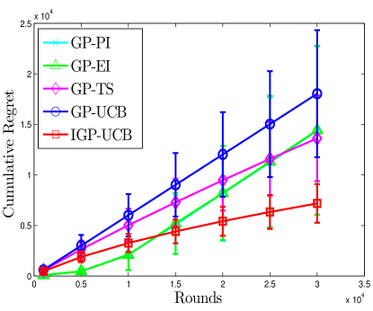
Figure 1: Cumulative regret for functions lying in the RKHS corresponding to (a) Squared Exponential kernel and (b) Mat$\acute{e}$rn kernel.

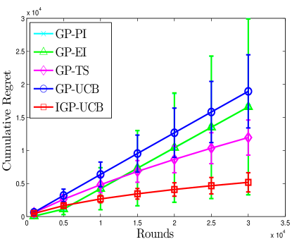
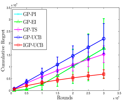
Figure 2: Cumulative regret for functions lying in the GP corresponding to (a) Squared Exponential kernel and (b) Mat$\acute{e}$rn kernel.

Standard Test Functions. We consider $2$ well-known synthetic benchmark functions for Bayesian Optimization: Rosenbrock and Hartman3 (see Azimi et al. (2012) for exact analytical expressions). We sample $100\;d$ points uniformly from the domain of each benchmark function, $d$ being the dimension of respective domain, as the decision set. We consider the Squared Exponential kernel with $l=0.2$ and set all parameters exactly as in previous experiment. The cumulative regret for $25$ independent trials on Rosenbrock and Hartman3 benchmarks is shown in Figure 3. We see GP-EI/PI perform better than the rest, while IGP-UCB and GP-TS show competitive performance. Here no algorithm is aware of the underlying kernel function, hence we conjecture that the UCB- and TS- based algorithms are somewhat less robust on the choice of kernel than EI/PI.

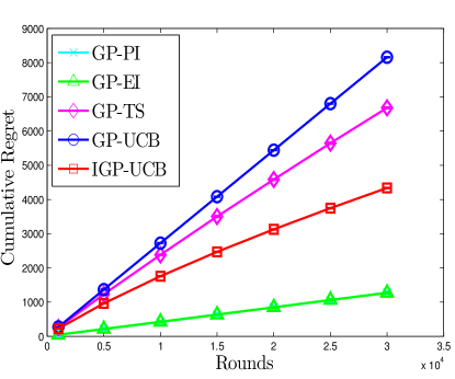
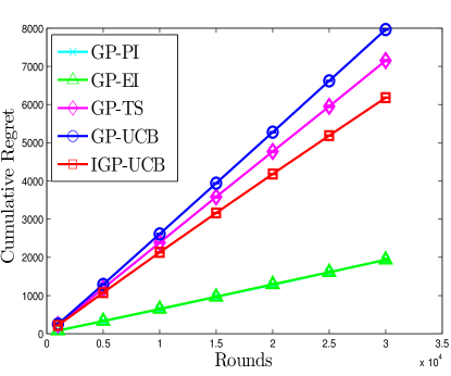
Figure 3: Cumulative regret for (a) Rosenbrock and (b) Hartman3 benchmark function.

Temperature Sensor Data. We use temperature data collected from 54 sensors deployed in the Intel Berkeley Research lab between February 28th and April 5th, 2004 with samples collected at 30 second intervals. We tested all algorithms in the context of learning the maximum reading of the sensors collected between 8 am to 9 am. We take measurements of first 5 consecutive days (starting Feb. 28th 2004) to learn algorithm parameters. Following Srinivas et al. (2009), we calculate the empirical covariance matrix of the sensor measurements and use it as the kernel matrix in the algorithms. Here $R^{2}$ is set to be $5\%$ of the average empirical variance of sensor readings and other algorithm parameters is set similarly as in the previous experiment with $\gamma_{t}=1$ (found via cross-validation). The functions for testing consist of one set of measurements from all sensors in the two following days and the cumulative regret is plotted over all such test functions. From Figure 4, we see that IGP-UCB and GP-UCB performs the same, while GP-TS outperforms all its competitors.

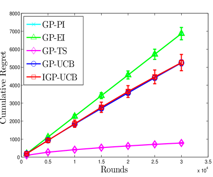
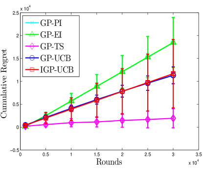
Figure 4: Cumulative regret plots for (a) temperature data and (b) light sensor data.

Light Sensor Data. We take light sensor data collected in the CMU Intelligent Workplace in Nov 2005, which is available online as Matlab structure and contains locations of $41$ sensors, $601$ train samples and $192$ test samples. We compute the kernel matrix, estimate the noise and set other algorithm parameters exactly as in the previous experiment. Here also GP-TS is found to perform better than the others, with IGP-UCB performing better than GP-EI/PI (Figure 4).

Related work. An alternative line of work pertaining to $\mathcal{X}$-armed bandits Kleinberg et al. (2008); Bubeck et al. (2011); Carpentier and Valko (2015); Azar et al. (2014) studies continuum-armed bandits with smoothness structure. For instance, Bubeck et al. (2011) show that with a Lipschitzness assumption on the reward function, algorithms based on discretizing the domain yield nontrivial regret guarantees, of order $\Omega(T^{\frac{d+1}{d+2}})$ in $\mathbb{R}^{d}$. Other Bayesian approaches to function optimization are GP-EI Močkus (1975), GP-PI Kushner (1964), GP-EST Wang et al. (2016) and GP-UCB, including the contextual Krause and Ong (2011), high-dimensional Djolonga et al. (2013); Wang et al. (2013), time-varying Bogunovic et al. (2016) safety-aware Gotovos et al. (2015), budget-constraint Hoffman et al. (2013) and noise-free De Freitas et al. (2012) settings. Other relevant work focuses on best arm identification problem in the Bayesian setup considering pure exploration Grünewälder et al. (2010). For Thompson sampling (TS), Russo and Van Roy (2014) analyze the Bayesian regret of TS, which includes the case where the target function is sampled from a GP prior. Our work obtains the first frequentist regret of TS for unknown, fixed functions from an RKHS.

7 Conclusion

For bandit optimization, we have improved upon the existing GP-UCB algorithm, and introduced a new GP-TS algorithm. The proposed algorithms perform well in practice both on synthetic and real-world data. An interesting case is when the kernel function is also not known to the algorithms a priori and needs to be learnt adaptively. Moreover, one can consider classes of time varying functions from the RKHS, and general reinforcement learning with GP techniques. There are also important questions on computational aspects of optimizing functions drawn from GPs.

Appendix

A. Proof of Theorem 1

For a function $g:D\rightarrow\mathbb{R}$ and a sequence of reals $n\equiv(n_{t})_{t=1}^{\infty}$, define for any $t\geq 0$

$$M_{t}^{g,n}=\exp\Big{(}\varepsilon_{1:t}^{T}g_{1:t,n}-\frac{R^{2}}{2}\left\lVert g_{1:t,n}\right\rVert^{2}\Big{)},$$

where the vector $g_{1:t,n}:=[g(x_{1})+n_{1},\ldots,g(x_{t})+n_{t}]^{T}$. We first establish the following technical result, which resembles Abbasi-Yadkori et al. (2011, Lemma 8).

Lemma 2

For fixed $g$ and $n$, $\{M_{t}^{g,n}\}_{t=0}^{\infty}$ is a super-martingale with respect to the filtration $\{\mathcal{F}_{t}\}_{t=0}^{\infty}$.

Proof  First, define

$$\Delta_{t}^{g,n}:=\exp\Big{(}\varepsilon_{t}(g(x_{t})+n_{t})-\frac{R^{2}}{2}(g(x_{t})+n_{t})^{2}\Big{)}.$$

Since $x_{t}$ is $\mathcal{F}_{t-1}$-measurable and $\varepsilon_{t}$ is $\mathcal{F}_{t}$-measurable, $M_{t}^{g,n}$ as well as $\Delta_{t}^{g,n}$ are $\mathcal{F}_{t}$ measurable. Also, by the conditional $R$-sub-Gaussianity of $\varepsilon_{t}$, we have

$$\forall\lambda\in\mathbb{R},\;\;\mathbb{E}\left[{e^{\lambda\varepsilon_{t}}\;\big{|}\;\mathcal{F}_{t-1}}\right]\leq\exp\left(\frac{\lambda^{2}R^{2}}{2}\right),$$

which in turn implies $\mathbb{E}\left[{\Delta_{t}^{g,n}\;\big{|}\;\mathcal{F}_{t-1}}\right]\leq 1$. We also have

$$\mathbb{E}\left[{M_{t}^{g,n}\;\big{|}\;\mathcal{F}_{t-1}}\right]$$

$$= \mathbb{E}\left[{M_{t-1}^{g,n}\Delta_{t}^{g,n}\;\big{|}\;\mathcal{F}_{t-1}}\right]=M_{t-1}^{g,n}\mathbb{E}\left[{\Delta_{t}^{g,n}\;\big{|}\;\mathcal{F}_{t-1}}\right]\leq M_{t-1}^{g,n},$$

showing that $\{M_{t}^{g,n}\}_{t=0}^{\infty}$ is a non-negative super-martingale and proving the lemma.  
Also observe that $\mathbb{E}\left[{M_{t}^{g,n}}\right]\leq 1$ for all $t$, as

$$\mathbb{E}\left[{M_{t}^{g,n}}\right]\leq\mathbb{E}\left[{M_{t-1}^{g,n}}\right]\leq\cdots\leq\mathbb{E}\left[{M_{0}^{g,n}}\right]=\mathbb{E}\left[{1}\right]=1.$$

Now, let $\tau$ be a stopping time with respect to the filtration $\{\mathcal{F}_{t}\}_{t=0}^{\infty}$. By the convergence theorem for nonnegative super-martingales (Durrett, 2005), $M_{\infty}^{g,n}=\lim\limits_{t\rightarrow\infty}M_{t}^{g,n}$ exists almost surely, and thus $M_{\tau}^{g,n}$ is well-defined. Now let $Q_{t}^{g,n}=M_{\min\{\tau,t\}}^{g,n}$, $t\geq 0$, be a stopped version of $\{M_{t}^{g,n}\}_{t}$. By Fatou’s lemma (Durrett, 2005),

$$\mathbb{E}\left[{M_{\tau}^{g,n}}\right] = \mathbb{E}\left[{\lim_{t\rightarrow\infty}Q_{t}^{g,n}}\right]=\mathbb{E}\left[{\liminf_{t\rightarrow\infty}Q_{t}^{g,n}}\right]$$ (8)

$$\leq \liminf_{t\rightarrow\infty}\mathbb{E}\left[{Q_{t}^{g,n}}\right]$$

$$= \liminf_{t\rightarrow\infty}\mathbb{E}\left[{M_{\min\{\tau,t\}}^{g,n}}\right]\leq 1,$$

since the stopped super-martingale $\left(M_{\min\{\tau,t\}}^{g,n}\right)_{t}$ is also a super-martingale (Durrett, 2005).

Now, let $\mathcal{F}_{\infty}$ be the $\sigma$-algebra generated by $\{\mathcal{F}_{t}\}_{t=0}^{\infty}$, and let $N\equiv(N_{t})_{t=1}^{\infty}$ be a sequence of independent and identically distributed Gaussian random variables with mean $0$ and variance $\eta$, independent of $\mathcal{F}_{\infty}$. Let $h:D\to\mathbb{R}$ be a random function distributed according to the Gaussian process measure $GP_{D}(0,k)$, and independent of both $\mathcal{F}_{\infty}$ and $(N_{t})_{t=1}^{\infty}$.

For each $t\geq 0$, define $M_{t}=\mathbb{E}\left[{M_{t}^{h,N}\;\big{|}\;\mathcal{F}_{\infty}}\right]$. In words, $(M_{t})_{t}$ is a mixture of super-martingales of the form $M_{t}^{g,n}$, and it is not hard to see that $(M_{t})_{t}$ is also a (non-negative) super-martingale w.r.t. the filtration $\{\mathcal{F}_{t}\}_{t}$, hence $M_{\infty}=\lim\limits_{t\rightarrow\infty}M_{t}$ is well-defined almost surely. We can write

$$\mathbb{E}\left[{M_{t}}\right]=\mathbb{E}\left[{M_{t}^{h,N}}\right]=\mathbb{E}\left[{\mathbb{E}\left[{M_{t}^{h,N}\;\big{|}\;h,N}\right]}\right]\leq\mathbb{E}\left[{1}\right]=1\;\;\forall t.$$

An argument similar to (8) also shows that $\mathbb{E}\left[{M_{\tau}}\right]\leq 1$ for any stopping time $\tau$. Now, without loss of generality, we assume $R=1$ (this can always be achieved through appropriate scaling), and compute

$$M_{t} = \mathbb{E}\left[{\exp\Big{(}\varepsilon_{1:t}^{T}h_{1:t,N}-\frac{1}{2}\left\lVert h_{1:t,N}\right\rVert^{2}\Big{)}\;\big{|}\;\mathcal{F}_{\infty}}\right]$$

$$= \int_{\mathbb{R}^{D}}\int_{\mathbb{R}^{t}}\exp\Big{(}\varepsilon_{1:t}^{T}([h(x_{1})\ldots h(x_{t})]^{T}+z)-\frac{1}{2}\left\lVert[h(x_{1})\ldots h(x_{t})]^{T}+z\right\rVert^{2}\Big{)}d\mu_{1}(h)d\mu_{2}(z)$$

$$= \int_{\mathbb{R}^{t}}\exp\Big{(}\varepsilon_{1:t}^{T}\lambda-\frac{1}{2}\left\lVert\lambda\right\rVert^{2}\Big{)}f(\lambda)d\lambda,$$

where $\mu_{1}$ is the Gaussian process measure $GP_{D}(0,k)$ over the function space $\mathbb{R}^{D}\equiv\{g:D\to\mathbb{R}\}$, $\mu_{2}$ is the multivariate Gaussian distribution on $\mathbb{R}^{t}$ with mean $0$ and covariance $\eta I$ where $I$ is the identify, $du$ is standard Lebesgue measure on $\mathbb{R}^{t}$, and $f$ is the density of the random vector $[h(x_{1})\ldots h(x_{t})]^{T}+z$, which is distributed as the multivariate Gaussian $\mathcal{N}(0,K_{t}+\eta I)$ given the sampled points $x_{1},\ldots,x_{t}$ up to round $t$, where $K_{t}$ is the induced kernel matrix at time $t$ given by $K_{t}(i,j)=k(x_{i},x_{j})$, $1\leq i,j\leq t$. (Note: $K_{t}$ is not positive definite and invertible when there are repetitions among $(x_{1},\ldots,x_{t})$, but $K_{t}+\eta I$ is).

Thus, we have

$$M_{t} =\frac{1}{\sqrt{(2\pi)^{t}\det(K_{t}+\eta I)}}\int_{\mathbb{R}^{t}}\exp\Bigg{(}\varepsilon_{1:t}^{T}\lambda-\frac{\left\lVert\lambda\right\rVert^{2}}{2}-\frac{\left\lVert\lambda\right\rVert^{2}_{(K_{t}+\eta I)^{-1}}}{2}\Bigg{)}d\lambda$$

$$= \frac{\exp\Big{(}\frac{\left\lVert\varepsilon_{1:t}\right\rVert^{2}}{2}\Big{)}}{\sqrt{(2\pi)^{t}\det(K_{t}+\eta I)}}\int_{\mathbb{R}^{t}}\exp\Bigg{(}-\frac{\left\lVert\lambda-\varepsilon_{1:t}\right\rVert^{2}}{2}-\frac{\left\lVert\lambda\right\rVert^{2}_{(K_{t}+\eta I)^{-1}}}{2}\Bigg{)}d\lambda.$$

Now for positive-definite matrices $P$ and $Q$

$$\left\lVert x-a\right\rVert_{P}^{2}+\left\lVert x\right\rVert_{Q}^{2}=\left\lVert x-(P+Q)^{-1}Pa\right\rVert_{P+Q}^{2}+\left\lVert a\right\rVert_{P}^{2}-\left\lVert Pa\right\rVert_{(P+Q)^{-1}}^{2}.$$

Therefore,

$$\left\lVert\lambda-\varepsilon_{1:t}\right\rVert_{I}^{2}+\left\lVert\lambda\right\rVert^{2}_{(K_{t}+\eta I)^{-1}}$$

$$= \left\lVert\lambda-(I+(K_{t}+\eta I)^{-1})^{-1}I\varepsilon_{1:t}\right\rVert_{I+(K_{t}+\eta I)^{-1}}^{2}+\left\lVert\varepsilon_{1:t}\right\rVert_{I}^{2}-\left\lVert I\varepsilon_{1:t}\right\rVert_{(I+(K_{t}+\eta I)^{-1})^{-1}}^{2},$$

which yields

$$M_{t} = \frac{1}{\sqrt{(2\pi)^{t}\det(K_{t}+\eta I)}}\exp\Big{(}\frac{1}{2}\left\lVert\varepsilon_{1:t}\right\rVert_{(I+(K_{t}+\eta I)^{-1})^{-1}}^{2}\Big{)}$$

$$\times\int_{\mathbb{R}^{t}}\exp\Big{(}-\frac{1}{2}\left\lVert\lambda-(I+(K_{t}+\eta I)^{-1})^{-1}\varepsilon_{1:t}\right\rVert^{2}_{I+(K_{t}+\eta I)^{-1}}\Big{)}d\lambda$$

$$= \frac{1}{\sqrt{\det(K_{t}+\eta I)\det((K_{t}+\eta I)^{-1}+I)}}\exp\Big{(}\frac{1}{2}\left\lVert\varepsilon_{1:t}\right\rVert_{(I+(K_{t}+\eta I)^{-1})^{-1}}^{2}\Big{)}$$

$$= \frac{1}{\sqrt{\det(I+K_{t}+\eta I)}}\exp\Big{(}\frac{1}{2}\left\lVert\varepsilon_{1:t}\right\rVert_{(I+(K_{t}+\eta I)^{-1})^{-1}}^{2}\Big{)},$$

since for any positive definite matrix $A\in\mathbb{R}^{t}$,

$$\int_{\mathbb{R}^{t}}\exp\Big{(}-\frac{1}{2}(x-a)^{T}A(x-a)\Big{)}dx=\int_{\mathbb{R}^{t}}\exp\Big{(}-\frac{1}{2}\left\lVert x-a\right\rVert_{A}^{2}\Big{)}dx=\sqrt{(2\pi)^{t}/\det(A)}.$$

Now as $\mathbb{E}\left[{M_{\tau}}\right]\leq 1$, using Markov’s inequality gives, for any $\delta\in(0,1)$,

$$\mathbb{P}\left[{\left\lVert\varepsilon_{1:\tau}\right\rVert_{((K_{\tau}+\eta I)^{-1}+I)^{-1}}^{2}>2\ln\Big{(}\sqrt{\det((1+\eta)I+K_{\tau})}/\delta\Big{)}}\right]$$ (9)

$$= \mathbb{P}\left[{M_{\tau}>1/\delta}\right]<\delta\mathbb{E}\left[{M_{\tau}}\right]\leq\delta.$$

To complete the proof, we now employ a stopping time construction as in Abbasi-Yadkori et al. (2011). For each $t\geq 0$, define the ‘bad’ event

$$B_{t}(\delta)=\Big{\{}\omega\in\Omega:\left\lVert\varepsilon_{1:t}\right\rVert_{((K_{t}+\eta I)^{-1}+I)^{-1}}^{2}>2\ln\Big{(}\sqrt{\det((1+\eta)I+K_{t})}/\delta\Big{)}\Big{\}},$$

so that

$$\mathbb{P}\left[{\bigcup\limits_{t\geq 0}B_{t}(\delta)}\right]$$

$$= \mathbb{P}\left[{\exists t\geq 0:\left\lVert\varepsilon_{1:t}\right\rVert_{((K_{t}+\eta I)^{-1}+I)^{-1}}^{2}\leq 2\ln\Big{(}\sqrt{\det((1+\eta)I+K_{t})}/\delta\Big{)}}\right],$$

which is the probability required to be bounded by $\delta$ in the statement of the theorem.

Let $\tau^{\prime}$ be the first time when the bad event $B_{t}(\delta)$ happens, i.e., $\tau^{\prime}(\omega):=\min\{t\geq 0:\omega\in B_{t}(\delta)\}$, with $\min\{\emptyset\}:=\infty$ by convention. Clearly, $\tau^{\prime}$ is a stopping time, and

$$\bigcup\limits_{t\geq 0}B_{t}(\delta)=\{\omega\in\Omega:\tau^{\prime}(\omega)<\infty\}.$$

Therefore, we can write

$$\mathbb{P}\left[{\bigcup\limits_{t\geq 0}B_{t}(\delta)}\right]$$

$$= \mathbb{P}\left[{\tau^{\prime}<\infty}\right]$$

$$= \mathbb{P}\left[{\left\lVert\varepsilon_{1:\tau^{\prime}}\right\rVert_{((K_{\tau^{\prime}}+\eta I)^{-1}+I)^{-1}}^{2}>2\ln\Big{(}\sqrt{\det((1+\eta)I+K_{\tau^{\prime}})}/\delta\Big{)},\tau^{\prime}<\infty}\right]$$

$$\leq \mathbb{P}\left[{\left\lVert\varepsilon_{1:\tau^{\prime}}\right\rVert_{((K_{\tau^{\prime}}+\eta I)^{-1}+I)^{-1}}^{2}>2\ln\Big{(}\sqrt{\det((1+\eta)I+K_{\tau^{\prime}})}/\delta\Big{)}}\right]\leq\delta,$$

by the inequality (9).

When $K_{t}$ is positive definite (and hence invertible) for each $t\geq 1$, one can use a similar construction as in Part 1, with $\eta=0$ (i.e., $N$ is the all-zeros sequence with probability 1), to recover the corresponding conclusion (6) with $\eta=0$.  

Proof of Lemma 1

Define, for each time $t$, the $t\times\infty$ matrix $\Phi_{t}:=[\varphi(x_{1})\cdots\varphi(x_{t})]^{T}$, and observe that $V_{t}=I+\Phi_{t}^{T}\Phi_{t}$ and $K_{t}=\Phi_{t}\Phi_{t}^{T}$. With this, we can compute

$$\left\lVert S_{t}\right\rVert^{2}_{V_{t}^{-1}} =S_{t}^{T}V_{t}^{-1}S_{t}=\sum_{s=1}^{t}\varepsilon_{s}\varphi(x_{s})^{T}\left(I+\Phi_{t}^{T}\Phi_{t}\right)^{-1}\sum_{s=1}^{t}\varepsilon_{s}\varphi(x_{s})$$

$$=\varepsilon_{1:t}^{T}\Phi_{t}\left(I+\Phi_{t}^{T}\Phi_{t}\right)^{-1}\Phi_{t}^{T}\varepsilon_{1:t}$$

$$=\varepsilon_{1:t}^{T}\Phi_{t}\Phi_{t}^{T}\left(\Phi_{t}\Phi_{t}^{T}+I\right)^{-1}\varepsilon_{1:t}$$

$$=\varepsilon_{1:t}^{T}K_{t}\left(K_{t}+I\right)^{-1}\varepsilon_{1:t}$$

$$=\varepsilon_{1:t}^{T}\left(K_{t}^{-1}+I\right)^{-1}\varepsilon_{1:t}=\left\lVert\varepsilon_{1:t}\right\rVert^{2}_{\left(K_{t}^{-1}+I\right)^{-1}},$$

completing the proof.

B. Information Theoretic Results

Lemma 3

For every $t\geq 0$, the maximum information gain $\gamma_{t}$, for the points chosen by Algorithm 1 and 2 satisfy, almost surely, the following :

$$\gamma_{t} \geq \frac{1}{2}\ln(\det(I+\lambda^{-1}K_{t})),$$

$$\gamma_{t} \geq \frac{1}{2}\sum_{s=1}^{t}\ln(1+\lambda^{-1}\sigma_{s-1}^{2}(x_{s})).$$

Proof  At round $t$ after observing the reward vector $y_{1:t}$ at points $A_{t}=\{x_{1},\ldots,x_{t}\}\subset D$, the information gain - by the algorithm - about the unknown reward function $f$ is given by the mutual information between $f_{1:t}$ and $y_{1:t}$ sampled at points $A_{t}$:

$$I(y_{1:t};f_{1:t})=H(y_{1:t})-H(y_{1:t}\;\big{|}\;f_{1:t}),$$

where $y_{1:t}=f_{1:t}+\varepsilon_{1:t}=[y_{1},\ldots,y_{t}]^{T}$, $f_{1:t}=[f(x_{1}),\ldots,f(x_{t})]^{T}$ and $\varepsilon_{1:t}=[\varepsilon_{1},\ldots,\varepsilon_{t}]^{T}$. Clearly, given $f_{1:t}$ the randomness - as perceived by the algorithm - in $y_{1:t}$ are only in the noise vector $\varepsilon_{1:t}$ and thus

$$H(y_{1:t}\;\big{|}\;f_{1:t})=\frac{1}{2}\ln(\det(2\pi e\lambda v^{2}I))\\ =\frac{t}{2}\log(2\pi e\lambda v^{2}),$$

as $\varepsilon_{1:t}$ is assumed to follow the distribution $\mathcal{N}(0,\lambda v^{2}I)$ and $H(\mathcal{N}(\mu,\Sigma))=\frac{1}{2}\ln(\det(2\pi e\Sigma))$. Now $y_{1:t}$ sampled at points $A_{t}$ is believed to be distributed as $\mathcal{N}(0,v^{2}(K_{t}+\lambda I))$, which gives $H(y_{1:t})=\frac{1}{2}\ln(\det(2\pi ev^{2}(\lambda I+K_{t})))=\frac{t}{2}\log(2\pi e\lambda v^{2})+\frac{1}{2}\ln(\det(I+\lambda^{-1}K_{t}))$, and therefore

$$I(y_{1:t};f_{1:t})=\frac{1}{2}\ln(\det(I+\lambda^{-1}K_{t})).$$ (10)

Again, conditioned on reward vector $y_{1:s-1}$ observed at points $A_{s-1}$, the reward $y_{s}$ at round $s$ observed at $x_{s}$ is believed to follow the distribution $\mathcal{N}(\mu_{s-1}(x_{s}),v^{2}(\lambda+\sigma_{s-1}^{2}(x_{s})))$, which gives $H(y_{s}\;\big{|}\;y_{1:s-1})=\frac{1}{2}\ln(2\pi ev^{2}(\lambda+\sigma_{s-1}^{2}(x_{s})))=\frac{1}{2}\ln(2\pi e\lambda v^{2})+\frac{1}{2}\ln(1+\lambda^{-1}\sigma_{s-1}^{2}(x_{s}))$. Now by chain rule $H(y_{1:t})=\sum_{s=1}^{t}H(y_{s}\;\big{|}\;y_{1:s-1})=\frac{t}{2}\ln(2\pi e\lambda v^{2})+\frac{1}{2}\sum_{s=1}^{t}\ln(1+\lambda^{-1}\sigma_{s-1}^{2}(x_{s}))$, and therefore

$$I(y_{1:t};f_{1:t})=\frac{1}{2}\sum_{s=1}^{t}\ln(1+\lambda^{-1}\sigma_{s-1}^{2}(x_{s})).$$ (11)

Now $I(y_{1:t};f_{1:t})$ is a function of $A_{t}\subset D$, the random points chosen by the algorithm and thus

$$I(y_{1:t};f_{1:t})\leq\max\limits_{A\subset D:\left|A\right|=t}I(y_{A};f_{A})=\gamma_{t},\;\;\text{a.s.},$$

Now the proof follows from Equation 10 and 11.  

Lemma 4

Let $x_{1},\ldots x_{t}$ be the points selected by the algorithms. The sum of predictive standard deviation at those points can be expressed in terms of the maximum information gain. More precisely,

$$\sum_{t=1}^{T}\sigma_{t-1}(x_{t})\leq\sqrt{4(T+2)\gamma_{T}}.$$

Proof  First note that, by Cauchy-Schwartz inequality, $\sum_{t=1}^{T}\sigma_{t-1}(x_{t})\leq\sqrt{T\sum_{t=1}^{t}\sigma_{t-1}^{2}(x_{t})}$. Now since $0\leq\sigma_{t-1}^{2}(x)\leq 1$ for all $x\in D$ and by our choice of $\lambda=1+\eta,\eta\geq 0$, we have $\lambda^{-1}\sigma_{t-1}^{2}(x_{t})\leq 2\ln(1+\lambda^{-1}\sigma_{t-1}^{2}(x_{t}))$, where in the last inequality we used the fact that for any $0\leq\alpha\leq 1$, $\ln(1+\alpha)\geq\alpha/2$. Thus we get $\sigma_{t-1}^{2}(x_{t})\leq 2\lambda\ln(1+\lambda^{-1}\sigma_{t-1}^{2}(x_{t}))$. This implies

$$\sum_{t=1}^{T}\sigma_{t-1}(x_{t})\leq\sqrt{2T\sum_{t=1}^{T}\lambda\ln(1+\lambda^{-1}\sigma_{t-1}^{2}(x_{t}))}\leq\sqrt{4T\lambda\sum_{t=1}^{T}\frac{1}{2}\ln(1+\sigma_{t-1}^{2}(x_{t}))}\leq\sqrt{4T(1+\eta)\gamma_{T}},$$

where the last inequality follows from Lemma 3. Now the result follows by choosing $\eta=2/T$.  

C. Proof of Theorem 2

First define $\varphi(x)$ as $k(x,\cdot)$, where $\varphi:\mathbb{R}^{d}\rightarrow H$ maps any point $x$ in the primal space $\mathbb{R}^{d}$ to the RKHS $H$ associated with kernel function $k$. For any two functions $g,h\in H$, define the inner product $\langle g,h\rangle_{k}$ as $g^{T}h$ and the RKHS norm $\left\lVert g\right\rVert_{k}$ as $\sqrt{g^{T}g}$. Now as the unknown reward function $f$ lies in the RKHS $H_{k}(D)$, these definitions along with reproducing property of the RKHS imply $f(x)=\langle f,k(x,\cdot)\rangle_{k}=\langle f,\varphi(x)\rangle_{k}=f^{T}\varphi(x)$ and $k(x,x^{\prime})=\langle k(x,\cdot),k(x^{\prime},\cdot)\rangle_{k}=\langle\varphi(x),\varphi(x^{\prime})\rangle_{k}=\varphi(x)^{T}\varphi(x^{\prime})$ for all $x,x^{\prime}\in D$. Now defining $\Phi_{t}:=\big{[}\varphi(x_{1})^{T},\ldots,\varphi(x_{t})^{T}\big{]}^{T}$, we get the kernel matrix $K_{t}=\Phi_{t}\Phi_{t}^{T}$, $k_{t}(x)=\Phi_{t}\varphi(x)$ for all $x\in D$ and $f_{1:t}=\Phi_{t}f$. Since the matrices $(\Phi_{t}^{T}\Phi_{t}+I)$ and $(\Phi_{t}\Phi_{t}^{T}+\lambda I)$ are strictly positive definite and $(\Phi_{t}^{T}\Phi_{t}+\lambda I)\Phi_{t}^{T}=\Phi_{t}^{T}(\Phi_{t}\Phi_{t}^{T}+\lambda I)$, we have

$$\Phi_{t}^{T}(\Phi_{t}\Phi_{t}^{T}+\lambda I)^{-1}=(\Phi_{t}^{T}\Phi_{t}+\lambda I)^{-1}\Phi_{t}^{T}.$$ (12)

Also from the definitions above $(\Phi_{t}^{T}\Phi_{t}+\lambda I)\varphi(x)=\Phi_{t}^{T}k_{t}(x)+\lambda\varphi(x)$, and thus from 12 we deduce that

$$\varphi(x)=\Phi_{t}^{T}(\Phi_{t}\Phi_{t}^{T}+\lambda I)^{-1}k_{t}(x)+\lambda(\Phi_{t}^{T}\Phi_{t}+\lambda I)^{-1}\varphi(x),$$

which gives

$$\varphi(x)^{T}\varphi(x)=k_{t}(x)^{T}(\Phi_{t}\Phi_{t}^{T}+\lambda I)^{-1}k_{t}(x)+\lambda\varphi(x)^{T}(\Phi_{t}^{T}\Phi_{t}+\lambda I)^{-1}\varphi(x).$$

This implies

$$\lambda\varphi(x)^{T}(\Phi_{t}^{T}\Phi_{t}+\lambda I)^{-1}\varphi(x)=k(x,x)-k_{t}(x)^{T}(K_{t}+\lambda I)^{-1}k_{t}(x)=\sigma_{t}^{2}(x)$$ (13)

Now observe that

$$\left|f(x)-k_{t}(x)^{T}(K_{t}+\lambda I)^{-1}f_{1:t}\right| = \left|\varphi(x)^{T}f-\varphi(x)^{T}\Phi_{t}^{T}(\Phi_{t}\Phi_{t}^{T}+\lambda I)^{-1}\Phi_{t}f\right|$$

$$= \left|\varphi(x)^{T}f-\varphi(x)^{T}(\Phi_{t}^{T}\Phi_{t}+\lambda I)^{-1}\Phi_{t}^{T}\Phi_{t}f\right|$$

$$= \left|\lambda\varphi(x)^{T}(\Phi_{t}^{T}\Phi_{t}+\lambda I)^{-1}f\right|$$

$$\leq \left\lVert\lambda(\Phi_{t}^{T}\Phi_{t}+\lambda I)^{-1}\varphi(x)\right\rVert_{k}\left\lVert f\right\rVert_{k}$$

$$= \left\lVert f\right\rVert_{k}\sqrt{\lambda\varphi(x)^{T}(\Phi_{t}^{T}\Phi_{t}+\lambda I)^{-1}\lambda I(\Phi_{t}^{T}\Phi_{t}+\lambda I)^{-1}\varphi(x)}$$

$$\leq B\sqrt{\lambda\varphi(x)^{T}(\Phi_{t}^{T}\Phi_{t}+\lambda I)^{-1}(\Phi_{t}^{T}\Phi_{t}+\lambda I)(\Phi_{t}^{T}\Phi_{t}+\lambda I)^{-1}\varphi(x)}$$

$$= B\;\sigma_{t}(x),$$

where the second equality uses 12, the first inequality is by Cauchy-Schwartz and the final equality is from 13. Again see that

$$\left|k_{t}(x)^{T}(K_{t}+\lambda I)^{-1}\varepsilon_{1:t}\right| = \left|\varphi(x)^{T}\Phi_{t}^{T}(\Phi_{t}\Phi_{t}^{T}+\lambda I)^{-1}\varepsilon_{1:t}\right|$$

$$= \left|\varphi(x)^{T}(\Phi_{t}^{T}\Phi_{t}+\lambda I)^{-1}\Phi_{t}^{T}\varepsilon_{1:t}\right|$$

$$\leq \left\lVert(\Phi_{t}^{T}\Phi_{t}+\lambda I)^{-1/2}\varphi(x)\right\rVert_{k}\left\lVert(\Phi_{t}^{T}\Phi_{t}+\lambda I)^{-1/2}\Phi_{t}^{T}\varepsilon_{1:t}\right\rVert_{k}$$

$$= \sqrt{\varphi(x)^{T}(\Phi_{t}^{T}\Phi_{t}+\lambda I)^{-1}\varphi(x)}\sqrt{(\Phi_{t}^{T}\varepsilon_{1:t})^{T}(\Phi_{t}^{T}\Phi_{t}+\lambda I)^{-1}\Phi_{t}^{T}\varepsilon_{1:t}}$$

$$= \lambda^{-1/2}\sigma_{t}(x)\sqrt{\varepsilon_{1:t}^{T}\Phi_{t}\Phi_{t}^{T}(\Phi_{t}\Phi_{t}^{T}+\lambda I)^{-1}\varepsilon_{1:t}}$$

$$= \lambda^{-1/2}\sigma_{t}(x)\sqrt{\varepsilon_{1:t}^{T}K_{t}(K_{t}+\lambda I)^{-1}\varepsilon_{1:t}}$$

where the second equality is from 12, the first inequality is by Cauchy-Schwartz and the fourth inequality uses both 12 and 13. Now recall that, at round $t$, the posterior mean function $\mu_{t}(x)=k_{t}(x)^{T}(K_{t}+\lambda I)^{-1}y_{1:t}=k_{t}(x)^{T}(K_{t}+\lambda I)^{-1}(f_{1:t}+\varepsilon_{1:t})$, where $f_{1:t}=\big{[}f(x_{1}),\ldots,f(x_{t})\big{]}^{T}$ and $\varepsilon_{1:t}=\big{[}\varepsilon_{1},\ldots,\varepsilon_{t}\big{]}^{T}$. Thus we have

$$\left|\mu_{t}(x)-f(x)\right| \leq \left|k_{t}(x)^{T}(K_{t}+\lambda I)^{-1}\varepsilon_{1:t}\right|+\left|f(x)-k_{t}(x)^{T}(K_{t}+\lambda I)^{-1}f_{1:t}\right|$$

$$\leq \sigma_{t}(x)\Big{(}B+(1+\eta)^{-1/2}\sqrt{\varepsilon_{1:t}^{T}K_{t}(K_{t}+(1+\eta)I)^{-1}\varepsilon_{1:t}}\Big{)},$$

where we have used $\lambda=1+\eta$, where $\eta\geq 0$ as stated in Theorem 1. Now observe that when $K$ is invertible, $K(K+I)^{-1}=((K+I)K^{-1})^{-1}=(I+K^{-1})^{-1}$. Using $K=K_{t}+\eta I$, we get

$$(K_{t}+\eta I)(K_{t}+(1+\eta)I)^{-1}=((K_{t}+\eta I)^{-1}+I)^{-1}.$$

Now see that

$$\varepsilon_{1:t}^{T}K_{t}(K_{t}+(1+\eta)I)^{-1}\varepsilon_{1:t}\leq\varepsilon_{1:t}^{T}(K_{t}+\eta I)(K_{t}+(1+\eta)I)^{-1}\varepsilon_{1:t}=\varepsilon_{1:t}^{T}((K_{t}+\eta I)^{-1}+I)^{-1}\varepsilon_{1:t}$$

Now using Theorem 1, for any $\delta\in(0,1)$, with probability at least $1-\delta$, $\forall t\geq 0,\forall x\in D$, we obtain

$$\left|\mu_{t}(x)-f(x)\right|\leq\sigma_{t}(x)\Big{(}B+\left\lVert\varepsilon_{1:t}\right\rVert_{(K_{t}+\eta I)^{-1}+I)^{-1}}\Big{)}\\ \leq\sigma_{t}(x)\Big{(}B+R\sqrt{2\ln\frac{\sqrt{\det((1+\eta)I+K_{t})}}{\delta}}\Big{)}.\\$$

Now observe that $\det((1+\eta)I+K_{t})=\det(I+(1+\eta)^{-1}K_{t})\det((1+\eta)I)$. Thus we have

$$\ln(\det((1+\eta)I+K_{t}))=\ln(\det(I+(1+\eta)^{-1}K_{t}))+t\ln(1+\eta)\leq 2\gamma_{t}+\eta t,$$

from lemma 3. Now choosing $\eta=2/T$ we have $\left|\mu_{t}(x)-f(x)\right|\leq\sigma_{t}(x)\Big{(}B+R\sqrt{2\big{(}\gamma_{t}+1+\ln(1/\delta)\big{)}}\Big{)}$ and hence the result follows.  

D. Analysis of IGP-UCB (Theorem 3)

Observe that at each round $t\geq 1$, by the choice of $x_{t}$ in Algorithm 1, we have $\mu_{t-1}(x_{t})+\beta_{t}\sigma_{t-1}(x_{t})\geq\mu_{t-1}(x^{\star})+\beta_{t}\sigma_{t-1}(x^{\star})$ and from Lemma 2, we have $f(x^{\star})\leq\mu_{t-1}(x^{\star})+\beta_{t}\sigma_{t-1}(x^{\star})$ and $\mu_{t-1}(x_{t})-f(x_{t})\leq\beta_{t}\sigma_{t-1}(x_{t})$. Therefore for all $t\geq 1$ with probability at least $1-\delta$,

$$r_{t} = f(x^{\star})-f(x_{t})$$

$$\leq \beta_{t}\sigma_{t-1}(x_{t})+\mu_{t-1}(x_{t})-f(x_{t})$$

$$\leq 2\beta_{t}\sigma_{t-1}(x_{t}),$$

and hence $\sum\limits_{t=1}^{T}r_{t}\leq 2\beta_{T}\sum\limits_{t=1}^{T}\sigma_{t-1}(x_{t})$. Now from Lemma 4, $\sum\limits_{t=1}^{T}\sigma_{t-1}(x_{t})=O(\sqrt{T\gamma_{T}})$ and by definition $\beta_{T}\leq B+R\sqrt{2(\gamma_{T}+1+\ln(1/\delta))}$. Hence with probability at least $1-\delta$,

$$R_{T}=\sum\limits_{t=1}^{T}r_{t}=O\Big{(}B\sqrt{T\gamma_{T}}+\sqrt{T\gamma_{T}(\gamma_{T}+\ln(1/\delta))}\Big{)},$$

and thus with high probability,

$$R_{T}=O\Big{(}\sqrt{T}(B\sqrt{\gamma_{T}}+\gamma_{T})\Big{)}.$$

E. Analysis of GP-TS (Theorem 4)

Lemma 5

For any $\delta\in(0,1)$ and any finite subset $D^{\prime}$ of $D$,

$$\mathbb{P}\Big{[}\forall x\in D^{\prime},\left|f_{t}(x)-\mu_{t-1}(x)\right|\leq v_{t}\sqrt{2\ln(\left|D^{\prime}\right|t^{2})}\;\sigma_{t-1}(x)\;\big{|}\;\mathcal{H}_{t-1}\Big{]}\geq 1-1/t^{2},$$

for all possible realizations of history $\mathcal{H}_{t-1}$.

Proof  Fix $x\in D$ and $t\geq 1$. Given history $\mathcal{H}_{t-1}$, $f_{t}(x)\sim\mathcal{N}(\mu_{t-1}(x),v_{t}^{2}\sigma_{t-1}^{2}(x))$. Thus using Lemma $B4$ of Hoffman et al. (2013), for any $\delta\in(0,1)$, with probability at least $1-\delta$

$$\left|f_{t}(x)-\mu_{t-1}(x)\right|\leq\sqrt{2\ln(1/\delta)}\;v_{t}\sigma_{t-1}(x),$$

and now applying union bound,

$$\left|f_{t}(x)-\mu_{t-1}(x)\right|\leq v_{t}\sqrt{2\ln(\left|D^{\prime}\right|/\delta)}\;\sigma_{t-1}(x)\;\;\forall x\in D^{\prime}$$

holds with probability at least $1-\delta$, given any possible realizations of history $\mathcal{H}_{t-1}$. Now setting $\delta=1/t^{2}$, the result follows.  

Definition 1

Define For all $t\geq 1$, $\tilde{c}_{t}=\sqrt{4\ln t+2d\ln(BLrdt^{2})}$ and $c_{t}=v_{t}(1+\tilde{c}_{t})$, where $v_{t}=B+R\sqrt{2(\gamma_{t-1}+1+\ln(2/\delta))}$. Clearly, $c_{t}$ increases with $t$.

Definition 2

Define $E^{f}(t)$ as the event that for all $x\in D$,

$$\left|\mu_{t-1}(x)-f(x)\right|\leq v_{t}\sigma_{t-1}(x),$$

and $E^{f_{t}}(t)$ as the event that for all $x\in D_{t}$,

$$\left|f_{t}(x)-\mu_{t-1}(x)\right|\leq v_{t}\tilde{c}_{t}\sigma_{t-1}(x).$$

Definition 3

Define the set of saturated points $S_{t}$ in discretization $D_{t}$ at round $t$ as

$$S_{t}:=\{x\in D_{t}:\Delta_{t}(x)>c_{t}\sigma_{t-1}(x)\},$$

where $\Delta_{t}(x):=f([x^{\star}]_{t})-f(x)$, the difference between function values at the closest point to $x^{\star}$ in $D_{t}$ and at $x$. Clearly $\Delta_{t}([x^{\star}]_{t})=0$ for all $t$, and hence $[x^{\star}]_{t}\in D_{t}$ is unsaturated at every $t$.

Definition 4

Define filtration $\mathcal{F}^{{}^{\prime}}_{t-1}$ as the history until time $t$, i.e., $\mathcal{F}^{{}^{\prime}}_{t-1}=\mathcal{H}_{t-1}$. By definition, $\mathcal{F}^{{}^{\prime}}_{1}\subseteq\mathcal{F}{{}^{\prime}}_{2}\subseteq\cdots$. Observe that given $\mathcal{F}^{{}^{\prime}}_{t-1}$, the set $S_{t}$ and the event $E^{f}(t)$ are completely deterministic.

Lemma 6

Given any $\delta\in(0,1)$, $\mathbb{P}\left[{\forall t\geq 1,E^{f}(t)}\right]\geq 1-\delta/2$ and for all possible filtrations $\mathcal{F}^{{}^{\prime}}_{t-1}$, $\mathbb{P}\left[{E^{f_{t}}(t)\;\big{|}\;\mathcal{F}^{{}^{\prime}}_{t-1}}\right]\geq 1-1/t^{2}$.

Proof  The probability bound for the event $E^{f}(t)$ follows from Theorem 2 by replacing $\delta$ with $\frac{\delta}{2}$ and for the event $E^{f_{t}}(t)$ follows from Lemma 5 by setting $D^{\prime}=D_{t}$ and $\mathcal{H}_{t-1}=\mathcal{F}^{{}^{\prime}}_{t-1}$.  

Lemma 7 (Gaussian Anti-concentration)

For a Gaussian random variable $X$ with mean $\mu$ and standard deviation $\sigma$, for any $\beta>0$,

$$\mathbb{P}\left[{\frac{X-\mu}{\sigma}>\beta}\right]\geq\frac{e^{-\beta^{2}}}{4\sqrt{\pi}\beta}.$$

Lemma 8

For any filtration $\mathcal{F}^{{}^{\prime}}_{t-1}$ such that $E^{f}(t)$ is true,

$$\mathbb{P}\left[{f_{t}(x)>f(x)\;\big{|}\;\mathcal{F}^{{}^{\prime}}_{t-1}}\right]\geq p,$$

for any $x\in D$, where $p=\frac{1}{4e\sqrt{\pi}}$.

Proof  Fix any $x\in D$. Given filtration $\mathcal{F}^{{}^{\prime}}_{t-1}$, $f_{t}(x)$ is a Gaussian random variable with mean $\mu_{t-1}(x)$ and standard deviation $v_{t}\sigma_{t-1}(x)$ and since event $E^{f}(t)$ is true, $\left|\mu_{t-1}(x)-f(x)\right|\leq c_{1,t}\sigma_{t-1}(x)$. Now using the anti-concentration inequality in Lemma 7, we have

$$\mathbb{P}\left[{f_{t}(x)>f(x)\;\big{|}\;\mathcal{F}^{{}^{\prime}}_{t-1}}\right] = \mathbb{P}\left[{\frac{f_{t}(x)-\mu_{t-1}(x)}{v_{t}\sigma_{t-1}(x)}>\frac{f(x)-\mu_{t-1}(x)}{v_{t}\sigma_{t-1}(x)}\;\big{|}\;\mathcal{F}^{{}^{\prime}}_{t-1}}\right]$$

$$\geq \mathbb{P}\left[{\frac{f_{t}(x)-\mu_{t-1}(x)}{v_{t}\sigma_{t-1}(x)}>\frac{\left|f(x)-\mu_{t-1}(x)\right|}{v_{t}\sigma_{t-1}(x)}\;\big{|}\;\mathcal{F}^{{}^{\prime}}_{t-1}}\right]$$

$$\geq \frac{1}{4\sqrt{\pi}\beta_{t}}e^{-\theta_{t}^{2}},$$

where, from Definition 2, $\theta_{t}=\frac{\left|f(x)-\mu_{t-1}(x)\right|}{v_{t}\sigma_{t-1}(x)}\leq 1$. Therefore $\mathbb{P}\left[{f_{t}(x)>f(x)\;\big{|}\;\mathcal{F}^{{}^{\prime}}_{t-1}}\right]\geq\frac{1}{4e\sqrt{\pi}}$, and hence the result follows.  

Lemma 9

For any filtration $\mathcal{F}^{{}^{\prime}}_{t-1}$ such that $E^{f}(t)$ is true,

$$\mathbb{P}\left[{x_{t}\in D_{t}\setminus S_{t}\;\big{|}\;\mathcal{F}^{{}^{\prime}}_{t-1}}\right]\geq p-1/t^{2}.$$

Proof  At round $t$ our algorithm chooses the point $x_{t}\in D_{t}$, at which the highest value of $f_{t}$, within current decision set $D_{t}$, is attained. Now if $f_{t}([x^{\star}]_{t})$ is greater than $f_{t}(x)$ for all saturated points at round $t$, i.e.,$f_{t}([x^{\star}]_{t})>f_{t}(x),\forall x\in S_{t}$, then one of the unsaturated points (which includes $[x^{\star}]_{t}$) in $D_{t}$ must be played and hence $x_{t}\in D_{t}\setminus S_{t}$. This implies

$$\mathbb{P}\left[{x_{t}\in D_{t}\setminus S_{t}\;\big{|}\;\mathcal{F}^{{}^{\prime}}_{t-1}}\right]\geq\mathbb{P}\left[{f_{t}([x^{\star}]_{t})>f_{t}(x),\forall x\in S_{t}\;\big{|}\;\mathcal{F}^{{}^{\prime}}_{t-1}}\right].$$ (14)

Now form Definition 3, $\Delta_{t}(x)>c_{t}\sigma_{t-1}(x)$, for all $x\in S_{t}$. Also if both the events $E^{f}(t)$ and $E^{f_{t}}(t)$ are true, then from Definition 1 and 2, $f_{t}(x)\leq f(x)+c_{t}\sigma_{t-1}(x)$, for all $x\in D_{t}$. Thus for all $x\in S_{t}$, $f_{t}(x)<f(x)+\Delta_{t}(x)$. Therefore, for any filtration $\mathcal{F}^{{}^{\prime}}_{t-1}$ such that $E^{f}(t)$ is true, either $E^{f_{t}}(t)$ is false, or else for all $x\in S_{t}$, $f_{t}(x)<f([x^{\star}]_{t})$. Hence, for any $\mathcal{F}^{{}^{\prime}}_{t-1}$ such that $E^{f}(t)$ is true,

$$\mathbb{P}\left[{f_{t}([x^{\star}]_{t})>f_{t}(x),\forall x\in S_{t}\;\big{|}\;\mathcal{F}^{{}^{\prime}}_{t-1}}\right]\\ \geq\mathbb{P}\left[{f_{t}([x^{\star}]_{t})>f([x^{\star}]_{t})\;\big{|}\;\mathcal{F}_{t-1}}\right]-\mathbb{P}\left[{\overline{E^{f_{t}}(t)}\;\big{|}\;\mathcal{F}^{{}^{\prime}}_{t-1}}\right]\\ \geq p-1/t^{2},$$

where we have used Lemma 6 and Lemma 8. Now the proof follows from Equation 14.  

Lemma 10

For any filtration $\mathcal{F}^{{}^{\prime}}_{t-1}$ such that $E^{f}(t)$ is true,

$$\mathbb{E}\left[{r_{t}\;\big{|}\;\mathcal{F}^{{}^{\prime}}_{t-1}}\right]\leq\frac{11c_{t}}{p}\mathbb{E}\left[{\sigma_{t-1}(x_{t})\;\big{|}\;\mathcal{F}^{{}^{\prime}}_{t-1}}\right]+\frac{2B+1}{t^{2}},$$

where $r_{t}$ is the instantaneous regret at round $t$.

Proof  Let $\bar{x}_{t}$ be the unsaturated point in $D_{t}$ with smallest $\sigma_{t-1}(x)$, i.e.,

$$\bar{x}_{t}=\mathop{\mathrm{argmin}}\limits_{x\in D_{t}\setminus S_{t}}\sigma_{t-1}(x).$$ (15)

Since $\sigma_{t-1}(\cdot)$ and $S_{t}$ are deterministic given $\mathcal{F}^{{}^{\prime}}_{t-1}$, so is $\bar{x}_{t}$. Now for any $\mathcal{F}^{{}^{\prime}}_{t-1}$ such that $E^{f}(t)$ is true,

$$\mathbb{E}\left[{\sigma_{t-1}(x_{t})\;\big{|}\;\mathcal{F}^{{}^{\prime}}_{t-1}}\right] \geq \mathbb{E}\left[{\sigma_{t-1}(x_{t})\;\big{|}\;\mathcal{F}^{{}^{\prime}}_{t-1},x_{t}\in D_{t}\setminus S_{t}}\right]\mathbb{P}\left[{x_{t}\in D_{t}\setminus S_{t}\;\big{|}\;\mathcal{F}^{{}^{\prime}}_{t-1}}\right]$$ (16)

$$\geq \sigma_{t-1}(\bar{x}_{t})(p-1/t^{2}),$$

where we have used Equation 15 and Lemma 9. Now, if both the events $E^{f}(t)$ and $E^{f_{t}}(t)$ are true, then from Definition 1 and 2, $f(x)-c_{t}\sigma_{t-1}(x)\leq f_{t}(x)\leq f(x)+c_{t}\sigma_{t-1}(x)$, for all $x\in D_{t}$. Using this observation along with Definition 3 and the facts that $f_{t}(x_{t})\geq f_{t}(x)$ for all $x\in D_{t}$ and $\bar{x}_{t}\in D_{t}\setminus S_{t}$, we have

$$\Delta_{t}(x_{t}) = f([x^{\star}]_{t})-f(\bar{x}_{t})+f(\bar{x}_{t})-f(x_{t})$$

$$\leq \Delta_{t}(\bar{x}_{t})+f_{t}(\bar{x}_{t})+c_{t}\sigma_{t-1}(\bar{x}_{t})-f_{t}(x_{t})+c_{t}\sigma_{t-1}(x_{t})$$

$$\leq c_{t}\sigma_{t-1}(\bar{x}_{t})+c_{t}\sigma_{t-1}(\bar{x}_{t})+c_{t}\sigma_{t-1}(x_{t})$$

$$\leq c_{t}\big{(}2\sigma_{t-1}(\bar{x}_{t})+c_{t}\sigma_{t-1}(x_{t})\big{)}.$$

Therefore, for any $\mathcal{F}^{{}^{\prime}}_{t-1}$ such that $E^{f}(t)$ is true, either $\Delta_{t}(x_{t})\leq c_{t}\big{(}2\sigma_{t-1}(\bar{x}_{t})+c_{t}\sigma_{t-1}(x_{t})\big{)}$, or $E^{f_{t}}(t)$ is false. Now from our assumption of bounded variance, for all $x\in D$, $\left|f(x)\right|\leq\left\lVert f\right\rVert_{k}k(x,x)\leq B$, and hence $\Delta_{t}(x)\leq 2\sup\limits_{x\in D}\left|f(x)\right|\leq 2B$. Thus, using Equation 16, we get

$$\mathbb{E}\left[{\Delta_{t}(x_{t})\;\big{|}\;\mathcal{F}^{{}^{\prime}}_{t-1}}\right] \leq \mathbb{E}\left[{c_{t}\big{(}2\sigma_{t-1}(\bar{x}_{t})+c_{t}\sigma_{t-1}(x_{t})\big{)}\;\big{|}\;\mathcal{F}^{{}^{\prime}}_{t-1}}\right]+2B\mathbb{P}\left[{\overline{E^{f_{t}}(t)}\;\big{|}\;\mathcal{F}^{{}^{\prime}}_{t-1}}\right]$$ (17)

$$\leq \frac{2c_{t}}{p-1/t^{2}}\mathbb{E}\left[{\sigma_{t-1}(x_{t})\;\big{|}\;\mathcal{F}^{{}^{\prime}}_{t-1}}\right]+c_{t}\mathbb{E}\left[{\sigma_{t-1}(x_{t})\;\big{|}\;\mathcal{F}^{{}^{\prime}}_{t-1}}\right]+\frac{2B}{t^{2}}$$

$$\leq \frac{11c_{t}}{p}\mathbb{E}\left[{\sigma_{t-1}(x_{t})\;\big{|}\;\mathcal{F}^{{}^{\prime}}_{t-1}}\right]+\frac{2B}{t^{2}},$$

where in the last inequality we used that $1/(p-1/t^{2})\leq 5/p$, which holds trivially for $t\leq 4$ and also holds for $t\geq 5$, as $t^{2}>5e\sqrt{\pi}$. Now using Equation 7, we have the instantaneous regret at round $t$,

$$r_{t}=f(x^{\star})-f([x^{\star}]_{t})+f([x^{\star}]_{t})-f(x_{t})\leq\frac{1}{t^{2}}+\Delta_{t}(x_{t}),$$

and then taking conditional expectation on both sides, the result follows from Equation 17.  

Definition 5

Let us define $Y_{0}=0$, and for all $t=1,\ldots,T$:

$$\bar{r}_{t} = r_{t}\cdot\mathbb{I}\{E^{f}(t)\},$$

$$X_{t} = \bar{r}_{t}-\frac{11c_{t}}{p}\sigma_{t-1}(x_{t})-\frac{2B+1}{t^{2}},$$

$$Y_{t} = \sum_{s=1}^{t}X_{s}.$$

Definition 6

A sequence of random variables $(Z_{t};t\geq 0)$ is called a super-martingale corresponding to a filtration $\mathcal{F}_{t}$, if for all $t$, $Z_{t}$ is $\mathcal{F}_{t}$-measurable, and for $t\geq 1$,

$$\mathbb{E}\left[{Z_{t}\;\big{|}\;\mathcal{F}_{t-1}}\right]\leq Z_{t-1}.$$

Lemma 11 (Azuma-Hoeffding Inequality)

If a super-martingale $(Z_{t};t\geq 0)$, corresponding to filtration $\mathcal{F}_{t}$, satisfies $\left|Z_{t}-Z_{t-1}\right|\leq\alpha_{t}$ for some constant $\alpha_{t}$, for all $t=1,\ldots,T$, then for any $\delta\geq 0$,

$$\mathbb{P}\left[{Z_{T}-Z_{0}\leq\sqrt{2\ln(1/\delta)\sum_{t=1}^{T}\alpha_{t}^{2}}\;}\right]\geq 1-\delta.$$

Lemma 12

$(Y_{t};t=0,...,T)$ is a super-martingale process with respect to filtration $\mathcal{F}^{{}^{\prime}}_{t}$.

Proof  From Definition 6, we need to prove that for all $t\in\{1,\ldots,T\}$ and any possible $\mathcal{F}^{{}^{\prime}}_{t-1}$, $\mathbb{E}\left[{Y_{t}-Y_{t-1}\;\big{|}\;\mathcal{F}^{{}^{\prime}}_{t-1}}\right]\leq 0$, i.e.

$$\mathbb{E}\left[{\bar{r}_{t}|\mathcal{F}^{{}^{\prime}}_{t-1}}\right]\leq\frac{11c_{t}}{p}\mathbb{E}\left[{\sigma_{t-1}(x_{t})|\mathcal{F}^{{}^{\prime}}_{t-1}}\right]+\frac{2B+1}{t^{2}}.$$ (18)

Now if $\mathcal{F}^{{}^{\prime}}_{t-1}$ such that $E^{f}(t)$ is false, then $\bar{r}_{t}=r_{t}\cdot\mathbb{I}\{E^{f}(t)\}=0$, and Equation 18 holds trivially. Moreover, for $\mathcal{F}^{{}^{\prime}}_{t-1}$ such that both $E^{f}(t)$ is true, Equation 18 follows from Lemma 10.  

Lemma 13

Given any $\delta\in(0,1)$, with probability at least $1-\delta$,

$$R_{T}=\sum_{t=1}^{T}r(t)=\frac{11c_{T}}{p}\sum_{t=1}^{T}\sigma_{t-1}(x_{t})+\frac{(2B+1)\pi^{2}}{6}+\frac{(4B+11)c_{T}}{p}\sqrt{2T\ln(2/\delta)},$$

where $T$ is the total number of rounds played.

Proof  First note that from Definition 5 for all $t=1,\ldots,T$,

$$\left|Y_{t}-Y_{t-1}\right|=\left|X_{t}\right|\leq\left|\bar{r}_{t}\right|+\frac{11c_{t}}{p}\sigma_{t-1}(x_{t})+\frac{2B+1}{t^{2}}.$$

Now as $\bar{r}_{t}\leq r_{t}\leq 2\sup\limits_{x\in D}\left|f(x)\right|\leq 2B$ and $\sigma^{2}_{t-1}(x_{t})\leq\sigma^{2}_{0}(x_{t})\leq 1$, we have

$$\left|Y_{t}-Y_{t-1}\right|\leq 2B+\frac{11c_{t}}{p}+\frac{2B+1}{t^{2}}\leq\frac{(4B+11)c_{t}}{p},$$

which follows from the fact that $2B\leq 2Bc_{t}/p$ and also $(2B+1)/t^{2}\leq 2Bc_{t}/p$. Thus, we can apply Azuma-Hoeffding inequality (Lemma 11) to obtain that with probability at least $1-\delta/2$,

$$\sum_{t=1}^{T}\bar{r}_{t} \leq \sum_{t=1}^{T}\frac{11c_{t}}{p}\sigma_{t-1}(x_{t})+\sum_{t=1}^{T}\frac{2B+1}{t^{2}}+\sqrt{2\ln(2/\delta)\sum_{t=1}^{T}\frac{(4B+11)^{2}c_{t}^{2}}{p^{2}}}$$

$$\leq \frac{11c_{T}}{p}\sum_{t=1}^{T}\sigma_{t-1}(x_{t})+\frac{(2B+1)\pi^{2}}{6}+\frac{(4B+11)c_{T}}{p}\sqrt{2T\ln(2/\delta)},$$

as by definition $c_{t}\leq c_{T}$ for all $t\in\{1,\ldots,T\}$. Now, as the event $E^{f}(t)$ holds holds for all $t$ with probability at least $1-\delta/2$ (see Lemma 6), then from Definition 5, $\bar{r}_{t}=r_{t}$ for all $t$ with probability at least $1-\delta/2$. Now by applying union bound, the result follows.  

Proof of Theorem 4

From Lemma 4 we have, $\sum\limits_{t=1}^{T}\sigma_{t-1}(x_{t})=O(\sqrt{T\gamma_{T}})$. Also from Definition 1,

$$C_{T} \leq B+R\sqrt{2(\gamma_{T}+1+\ln(2/\delta))}+\Big{(}B+R\sqrt{2(\gamma_{T}+1+\ln(2/\delta))}\Big{)}\sqrt{4\ln T+2d\ln(BLrdT^{2})}$$

$$= O\Big{(}\sqrt{(\gamma_{T}+\ln(2/\delta))(\ln T+d\ln(BdT))}+B\sqrt{d\ln(BdT)}\Big{)}$$

$$= O\Big{(}\sqrt{(\gamma_{T}+\ln(2/\delta))d\ln(BdT)}\Big{)}.$$

Hence, from Lemma 13, with probability at least $1-\delta$,

$$R_{T}=O\Bigg{(}\sqrt{(\gamma_{T}+\ln(2/\delta))d\ln(BdT)}\cdot\Big{(}\sqrt{T\gamma_{T}}+B\sqrt{T\ln(2/\delta)}\Big{)}\Bigg{)}$$

and thus with high probability,

$$R_{T} = O\Big{(}\sqrt{T\gamma_{T}^{2}d\ln(BdT)}+B\sqrt{T\gamma_{T}d\ln(BdT)}\Big{)}$$

$$= O\Bigg{(}\sqrt{Td\ln(BdT)}\Big{(}B\sqrt{\gamma_{T}}+\gamma_{T}\Big{)}\Bigg{)}.\hskip 75.0pt$$

F. Recursive Updates of Posterior Mean and Covariance

We now describe a procedure to update the posterior mean and covariance function in a recursive fashion through the properties of Schur complement (Zhang (2006)) rather than evaluating Equation 2 and 3 at each round. Specifically for all $t\geq 1$ we show the following:

$$\mu_{t}(x) = \mu_{t-1}(x)+\dfrac{k_{t-1}(x,x_{t})}{\lambda+\sigma^{2}_{t-1}(x_{t})}(y_{t}-\mu_{t-1}(x_{t})),$$ (19)

$$k_{t}(x,x^{\prime}) = k_{t-1}(x,x^{\prime})-\dfrac{k_{t-1}(x,x_{t})k_{t-1}(x_{t},x^{\prime})}{\lambda+\sigma^{2}_{t-1}(x_{t})},$$ (20)

$$\sigma^{2}_{t}(x) = \sigma^{2}_{t-1}(x)-\dfrac{k^{2}_{t-1}(x,x_{t})}{\lambda+\sigma^{2}_{t-1}(x_{t})}.$$ (21)

These update rules make our algorithms easy to implement and we are not aware of any literature which explicitly states or uses these relations.

First we write the matrix $K_{t}+\lambda I$ as $\begin{bmatrix}A&B\\ C&D\end{bmatrix}$, where $A=K_{t-1}+\lambda I$, $B=k_{t-1}(x_{t})$, $C=B^{T}$ and $D=\lambda+k(x_{t},x_{t})$. Now using Schur’s complement we get

$$\begin{bmatrix}A&B\\ C&D\end{bmatrix}^{-1} = \begin{bmatrix}A^{-1}+A^{-1}B\beta CA^{-1}&-A^{-1}B\beta\\ -\beta CA^{-1}&\beta\end{bmatrix}$$

$$= \begin{bmatrix}A^{-1}+\beta A^{-1}BB^{T}A^{-1}&-\beta A^{-1}B\\ -\beta B^{T}A^{-1}&\beta\end{bmatrix}$$

$$= \begin{bmatrix}A^{-1}+\beta\gamma&-\beta\alpha\\ -\beta\alpha^{T}&\beta\end{bmatrix},$$

where $\beta=(D-CA^{-1}B)^{-1}=1/(D-B^{T}A^{-1}B)$, $\gamma=A^{-1}BB^{T}A^{-1}$ and $\alpha=A^{-1}B$. Therefore we have

$$\mu_{t}(x) = k_{t}(x)^{T}(K_{t}+\lambda I)^{-1}y_{1:t}$$

$$= \begin{bmatrix}k_{t-1}(x)^{T}&k(x_{t},x)\end{bmatrix}\begin{bmatrix}A^{-1}+\beta\gamma&-\beta\alpha\\ -\beta\alpha^{T}&\beta\end{bmatrix}\begin{bmatrix}y_{1:{t-1}}\\ y_{t}\end{bmatrix}$$

$$= k_{t-1}(x)^{T}(A^{-1}+\beta\gamma)y_{1:{t-1}}-\beta k(x_{t},x)\alpha^{T}y_{1:{t-1}}-\beta y_{t}\alpha^{T}k_{t-1}(x)+\beta y_{t}k(x_{t},x)$$

$$= k_{t-1}(x)^{T}A^{-1}y_{1:{t-1}}+\beta\Big{(}k_{t-1}(x)^{T}\gamma y_{1:{t-1}}-k(x_{t},x)\alpha^{T}y_{1:{t-1}}-y_{t}\alpha^{T}k_{t-1}(x)+y_{t}k(x_{t},x)\Big{)},$$

where

$$k_{t-1}(x)^{T}A^{-1}y_{1:{t-1}} = k_{t-1}(x)^{T}(K_{t-1}+\lambda I)^{-1}y_{1:{t-1}}=\mu_{t-1}(x),$$

$$k_{t-1}(x)^{T}\gamma y_{1:{t-1}} = k_{t-1}(x)^{T}A^{-1}k_{t-1}(x_{t})k_{t-1}(x_{t})^{T}A^{-1}y_{1:{t-1}}=\left(k_{t-1}(x_{t})^{T}A^{-1}k_{t-1}(x)\right)\mu_{t-1}(x_{t}),$$

$$\alpha^{T}y_{1:{t-1}} = k_{t-1}(x_{t})^{T}A^{-1}y_{1:{t-1}}=\mu_{t-1}(x_{t}),$$

$$\alpha^{T}k_{t-1}(x) = k_{t-1}(x_{t})^{T}A^{-1}k_{t-1}(x).$$

Thus we have

$$\mu_{t}(x) = \mu_{t-1}(x)+\beta\Big{(}k_{t-1}(x_{t})^{T}A^{-1}k_{t-1}(x)\left(\mu_{t-1}(x_{t})-y_{t}\right)+k(x_{t},x)\left(y_{t}-\mu_{t-1}(x_{t})\right)\Big{)}$$

$$= \mu_{t-1}(x)+\beta\left(y_{t}-\mu_{t-1}(x_{t})\right)\left(k(x_{t},x)-k_{t-1}(x_{t})^{T}A^{-1}k_{t-1}(x)\right)$$

$$= \mu_{t-1}(x)+\beta k_{t-1}(x_{t},x)(y_{t}-\mu_{t-1}(x_{t})).$$

Now as

$$D-B^{T}A^{-1}B=\lambda+k(x_{t},x_{t})-k_{t-1}(x_{t})^{T}(K_{t-1}+\lambda I)^{-1}k_{t-1}(x_{t})=\lambda+\sigma_{t-1}^{2}(x_{t}),$$

putting $\beta=1/(\lambda+\sigma^{2}_{t-1}(x_{t}))$, we obtain Equation 19. Again observe that

$$k_{t}(x,x^{\prime})$$

$$= k(x,x^{\prime})-k_{t}(x)^{T}(K_{t}+\lambda I)^{-1}k_{t}(x^{\prime})$$

$$= k(x,x^{\prime})-k_{t-1}(x)^{T}A^{-1}k_{t-1}(x^{\prime})$$

$$+\beta\Big{(}k_{t-1}(x)^{T}\gamma k_{t-1}(x^{\prime})-k(x_{t},x)\alpha^{T}k_{t-1}(x^{\prime})-k(x_{t},x^{\prime})\alpha^{T}k_{t-1}(x)+k(x_{t},x)k(x_{t},x^{\prime})\Big{)}.$$

Now we have

$$k(x,x^{\prime})-k_{t-1}(x)^{T}A^{-1}k_{t-1}(x^{\prime})=k(x,x^{\prime})-k_{t-1}(x)^{T}(K_{t-1}+\lambda I)^{-1}k_{t-1}(x^{\prime})=k_{t-1}(x,x^{\prime}),$$

also

$$k_{t-1}(x)^{T}\gamma k_{t-1}(x^{\prime})-k(x_{t},x)\alpha^{T}k_{t-1}(x^{\prime})$$

$$= k_{t-1}(x)^{T}A^{-1}k_{t-1}(x_{t})k_{t-1}(x_{t})^{T}A^{-1}k_{t-1}(x^{\prime})-k(x_{t},x)k_{t-1}(x_{t})^{T}A^{-1}k_{t-1}(x^{\prime})$$

$$= (k_{t-1}(x)^{T}A^{-1}k_{t-1}(x_{t})-k(x_{t},x))k_{t-1}(x_{t})^{T}A^{-1}k_{t-1}(x^{\prime})$$

$$= -k_{t-1}(x_{t},x)k_{t-1}(x_{t})^{T}A^{-1}k_{t-1}(x^{\prime}),$$

and

$$k(x_{t},x)k(x_{t},x^{\prime})-k(x_{t},x^{\prime})\alpha^{T}k_{t-1}(x) = k(x_{t},x^{\prime})(k(x_{t},x)-k_{t-1}(x_{t})^{T}A^{-1}k_{t-1}(x))$$

$$= k(x_{t},x^{\prime})k_{t-1}(x_{t},x).$$

Putting all these together we get

$$k_{t}(x,x^{\prime}) = k_{t-1}(x,x^{\prime})-\beta\Big{(}k(x_{t},x^{\prime})k_{t-1}(x_{t},x)-k_{t-1}(x_{t},x)k_{t-1}(x_{t})^{T}A^{-1}k_{t-1}(x^{\prime})\Big{)}$$

$$= k_{t-1}(x,x^{\prime})-\beta\Big{(}k_{t-1}(x_{t},x)\Big{(}k(x_{t},x^{\prime})-k_{t-1}(x_{t})^{T}A^{-1}k_{t-1}(x^{\prime})\Big{)}\Big{)}$$

$$= k_{t-1}(x,x^{\prime})-\beta k_{t-1}(x_{t},x)k_{t-1}(x_{t},x^{\prime}).$$

Now Equation 20 and 21 follows by using $\beta=1/(\lambda+\sigma^{2}_{t-1}(x))$ and $\sigma_{t}^{2}(x)=k_{t}(x,x)$.

References

- Abbasi-Yadkori et al. (2011) Yasin Abbasi-Yadkori, Dávid Pál, and Csaba Szepesvári. Improved algorithms for linear stochastic bandits. In Advances in Neural Information Processing Systems, pages 2312–2320, 2011.
- Agrawal and Goyal (2012) Shipra Agrawal and Navin Goyal. Analysis of thompson sampling for the multi-armed bandit problem. In COLT, pages 39–1, 2012.
- Agrawal and Goyal (2013) Shipra Agrawal and Navin Goyal. Thompson sampling for contextual bandits with linear payoffs. In ICML, pages 127–135, 2013.
- Azar et al. (2014) Mohammad Gheshlaghi Azar, Alessandro Lazaric, and Emma Brunskill. Online stochastic optimization under correlated bandit feedback. In ICML, pages 1557–1565, 2014.
- Azimi et al. (2012) Javad Azimi, Ali Jalali, and Xiaoli Fern. Hybrid batch bayesian optimization. arXiv preprint arXiv:1202.5597, 2012.
- Besbes and Zeevi (2009) Omar Besbes and Assaf Zeevi. Dynamic pricing without knowing the demand function: Risk bounds and near-optimal algorithms. Operations Research, 57(6):1407–1420, 2009.
- Bogunovic et al. (2016) Ilija Bogunovic, Jonathan Scarlett, and Volkan Cevher. Time-varying gaussian process bandit optimization. arXiv preprint arXiv:1601.06650, 2016.
- Bubeck et al. (2011) Sébastien Bubeck, Rémi Munos, Gilles Stoltz, and Csaba Szepesvári. X-armed bandits. Journal of Machine Learning Research, 12(May):1655–1695, 2011.
- Carpentier and Valko (2015) Alexandra Carpentier and Michal Valko. Simple regret for infinitely many armed bandits. In ICML, pages 1133–1141, 2015.
- Chiang et al. (2008) Mung Chiang, Prashanth Hande, Tian Lan, and Chee Wei Tan. Power control in wireless cellular networks. Foundations and Trends in Networking, 2(4):381–533, 2008. ISSN 1554-057X. doi: 10.1561/1300000009.
- Dani et al. (2008) Varsha Dani, Thomas P Hayes, and Sham M Kakade. Stochastic linear optimization under bandit feedback. In COLT, pages 355–366, 2008.
- De Freitas et al. (2012) Nando De Freitas, Alex Smola, and Masrour Zoghi. Exponential regret bounds for gaussian process bandits with deterministic observations. arXiv preprint arXiv:1206.6457, 2012.
- de la Pena et al. (2009) Victor H de la Pena, Tze Leung Lai, and Qi-Man Shao. Self-normalized processes. probability and its applications, 2009.
- Djolonga et al. (2013) Josip Djolonga, Andreas Krause, and Volkan Cevher. High-dimensional gaussian process bandits. In Advances in Neural Information Processing Systems, pages 1025–1033, 2013.
- Durrett (2005) Rick Durrett. Probability: Theory and Examples. Brooks/Cole - Thomson Learning, Belmont, CA, 2005.
- Gopalan et al. (2014) Aditya Gopalan, Shie Mannor, and Yishay Mansour. Thompson sampling for complex online problems. In ICML, volume 14, pages 100–108, 2014.
- Gotovos et al. (2015) Alkis Gotovos, ETHZ CH, and Joel W Burdick. Safe exploration for optimization with gaussian processes. 2015.
- Grünewälder et al. (2010) Steffen Grünewälder, Jean-Yves Audibert, Manfred Opper, and John Shawe-Taylor. Regret bounds for gaussian process bandit problems. In AISTATS, pages 273–280, 2010.
- Hoffman et al. (2011) Matthew D Hoffman, Eric Brochu, and Nando de Freitas. Portfolio allocation for bayesian optimization. In UAI, pages 327–336, 2011.
- Hoffman et al. (2013) Matthew W Hoffman, Bobak Shahriari, and Nando de Freitas. Exploiting correlation and budget constraints in bayesian multi-armed bandit optimization. arXiv preprint arXiv:1303.6746, 2013.
- Kaelbling et al. (1996) Leslie Pack Kaelbling, Michael L Littman, and Andrew W Moore. Reinforcement learning: A survey. Journal of artificial intelligence research, 4:237–285, 1996.
- Kaufmann et al. (2012) Emilie Kaufmann, Nathaniel Korda, and Rémi Munos. Thompson sampling: An asymptotically optimal finite-time analysis. In International Conference on Algorithmic Learning Theory, pages 199–213. Springer, 2012.
- Kleinberg et al. (2008) Robert Kleinberg, Aleksandrs Slivkins, and Eli Upfal. Multi-armed bandits in metric spaces. In Proceedings of the fortieth annual ACM symposium on Theory of computing, pages 681–690. ACM, 2008.
- Krause and Ong (2011) Andreas Krause and Cheng S Ong. Contextual gaussian process bandit optimization. In Advances in Neural Information Processing Systems, pages 2447–2455, 2011.
- Kushner (1964) Harold J Kushner. A new method of locating the maximum point of an arbitrary multipeak curve in the presence of noise. Journal of Basic Engineering, 86(1):97–106, 1964.
- Maillard (2016) Odalric-Ambrym Maillard. Self-normalization techniques for streaming confident regression. 2016.
- Močkus (1975) J Močkus. On bayesian methods for seeking the extremum. In Optimization Techniques IFIP Technical Conference, pages 400–404. Springer, 1975.
- Rasmussen and Williams (2006) Carl Edward Rasmussen and Christopher KI Williams. Gaussian processes for machine learning. 2006.
- Rusmevichientong and Tsitsiklis (2010) Paat Rusmevichientong and John N. Tsitsiklis. Linearly parameterized bandits. Math. Oper. Res., 35(2):395–411, May 2010.
- Russo and Van Roy (2014) Daniel Russo and Benjamin Van Roy. Learning to optimize via posterior sampling. Mathematics of Operations Research, 39(4):1221–1243, 2014.
- Schölkopf and Smola (2002) Bernhard Schölkopf and Alexander J Smola. Learning with kernels: support vector machines, regularization, optimization, and beyond. MIT press, 2002.
- Smart and Kaelbling (2000) William D Smart and Leslie Pack Kaelbling. Practical reinforcement learning in continuous spaces. In ICML, pages 903–910, 2000.
- Srinivas et al. (2009) Niranjan Srinivas, Andreas Krause, Sham M Kakade, and Matthias Seeger. Gaussian process optimization in the bandit setting: No regret and experimental design. arXiv preprint arXiv:0912.3995, 2009.
- Valko et al. (2013) Michal Valko, Nathaniel Korda, Rémi Munos, Ilias Flaounas, and Nelo Cristianini. Finite-time analysis of kernelised contextual bandits. arXiv preprint arXiv:1309.6869, 2013.
- Wang et al. (2016) Zi Wang, Bolei Zhou, and Stefanie Jegelka. Optimization as estimation with gaussian processes in bandit settings. In International Conf. on Artificial and Statistics (AISTATS), 2016.
- Wang et al. (2013) Ziyu Wang, Masrour Zoghi, Frank Hutter, David Matheson, N Freitas, et al. Bayesian optimization in high dimensions via random embeddings. AAAI Press/International Joint Conferences on Artificial Intelligence, 2013.
- Zhang (2006) Fuzhen Zhang. The Schur complement and its applications, volume 4. Springer Science & Business Media, 2006.