Ultra-Dense Networks: Is There a Limit to
Spatial Spectrum Reuse?

Abstract

The aggressive spatial spectrum reuse (SSR) by network densification using smaller cells has successfully driven the wireless communication industry onward in the past decades. In our future journey toward ultra-dense networks (UDNs), a fundamental question needs to be answered. Is there a limit to SSR? In other words, when we deploy thousands or millions of small cell base stations (BSs) per square kilometer, is activating all BSs on the same time/frequency resource the best strategy? In this paper, we present theoretical analyses to answer such question. In particular, we find that both the signal and interference powers become bounded in practical UDNs with a non-zero BS-to-UE antenna height difference and a finite UE density, which leads to a constant capacity scaling law. As a result, there exists an optimal SSR density that can maximize the network capacity. Hence, the limit to SSR should be considered in the operation of future UDNs.

I Introduction

From 1950 to 2000, the wireless network capacity has increased around 1 million fold, in which an astounding 2700× gain was achieved through an aggressive spatial spectrum reuse (SSR) via network densification using smaller cells [1]. Generally speaking, SSR means that all the cells in the area of interest simultaneously reuse the same frequency spectrum. Thus, the wireless network capacity has the potential to grow linearly as the SSR increases, as each cell can make an independent and equal contribution to it, given that the inter-cell interference remains tolerable. The aforementioned 2700× gain stands as a glorious testimony to the fulfillment of such potential.

In the first decade of 2000, network densification continued to fuel the 3rd Generation Partnership Project (3GPP) 4th-generation (4G) Long Term Evolution (LTE) networks, and is expected to remain as one of the main forces to drive the 5th-generation (5G) New Radio (NR) beyond 2020 [2]. In particular, the orthogonal deployment of dense small cell networks (SCNs), in which small cells and macrocells operate in different frequency bands [2], have gained much momentum in the past years. This is because such deployment provides a large SSR with easy network management due to the avoidance of inter-tier interference.

However, as we walk down the path of network densification, and gradually enter the realm of ultra-dense networks (UDNs), things start to deviate from the traditional understanding. In particular, several fundamental questions arise:

• The signal power of a typical user equipment (UE) should increase as a network goes ultra-dense. But is there a limit to such increase of the signal power?

• The aggregate interference power of the typical UE should also increase as a network goes ultra-dense. But is there a limit to such increase of the aggregate interference power?

• Which component will grow faster as a network densifies, the signal or the aggregate interference power?

• More importantly, is there a limit to the SSR? In other words, when we deploy thousands or millions of small cell base stations (BSs) per square kilometer, is activating all BSs on the same time/frequency resource the best strategy, as we have practiced in the last half century? Should we explore alternative solutions?

In this paper, we answer this fundamental question via theoretical analyses.

II Related Work

Before 2015, the common understanding on UDNs was that the density of BSs would not affect the per-BS coverage probability performance [3] in an interference-limited and fully-loaded wireless network, where the coverage probability is defined as the probability that the signal-to-interference-plus-noise ratio (SINR) of a typical UE is above a SINR threshold $\gamma$. Such phenomenon is referred to as the SINR invariance. The intuition of the SINR invariance is that the increase in the aggregate interference power caused by a denser network would be exactly compensated by the increase in the signal power due to the reduced distance between transmitters and receivers [3]. Consequently, the network capacity should scale linearly as the BS density increases in a fully-loaded UDN. Such conclusion, however, was obtained with considerable simplifications on network conditions and propagation environment.

Recently, a few noteworthy studies have followed and revisited the network performance analysis of UDNs using more practical assumptions [5, 6, 7, 8, 9, 10], such as

• a general multi-piece path loss model with probabilistic line-of-sight (LoS) and non-LoS (NLoS) transmissions,

• a non-zero BS-to-UE antenna height difference $L$, and

• a non-fully-loaded network with a finite UE density $\rho$.

The inclusion of these more realistic assumptions significantly changed the previous conclusion on the SINR invariance [3], indicating that the coverage probability performance of UDNs is neither a convex nor a concave function with respect to the BS density. In particular, two seemingly contradictory performance behaviors can be observed in [9] and [10], both considering a general multi-piece path loss model recommended by the 3GPP.

First, if we consider a practical non-zero BS-to-UE antenna height difference $L$, then the coverage probability is shown to crash as the BS density increases in a fully-loaded UDN. This is caused by a severe SINR decrease in UDNs [9]. The intuition of such SINR decrease is that the signal power becomes bounded in UDNs due to the lower-bound on the BS-to-UE distance, as a UE cannot be closer than $L$ to its serving BS.

Second, if we consider a practical finite UE density $\rho$, then the coverage probability is shown to take off as the BS density increases. This is caused by a soaring SINR increase in UDNs [10]. The intuition of such SINR increase is that the aggregate interference power becomes bounded in UDNs due to the partial activation of a finite density of BSs to serve a finite density of UEs. In more detail, a large number of BSs can switch off their transmission modules in UDNs, entering into idle mode, if there is no active UE within their coverage areas. As a result, the number of interfering BSs and also the SSR are limited by the finite number of UEs.

Considering that the above two seemingly contradictory performance behaviors (i.e., SINR decrease and increase) manifest themselves in UDNs, it is of great interest to investigate their trade-offs. Which one prevails in UDNs? Such study will eventually reveal the answer to the fundamental question: Is there a limit to the SSR? Our short answer is YES.

III Network Scenario and System Model

In this section, we present the network scenario and the wireless system model considered in this paper.

III-A Network Scenario

We consider a downlink (DL) cellular network with BSs deployed on a plane according to a homogeneous Poisson point process (HPPP) $\Phi$ with a density of $\lambda$ $\textrm{BSs/km}^{2}$. Active DL UEs are also Poisson distributed in the considered network with a density of $\rho$ $\textrm{UEs/km}^{2}$. Here, we only consider active UEs in the network because non-active UEs do not trigger any data transmission, the typical density of which is around $\rho=300\thinspace\textrm{UEs/km}^{2}$ [2].

In practice, a BS will enter an idle mode if there is no UE connected to it, which reduces the interference to neighboring UEs as well as the energy consumption of the network. The set of active BSs is thus depending on the user association strategy (UAS). In this paper, we assume a practical UAS as in [7], where each UE is connected to the BS having the maximum average received signal strength, which will be formally presented in Subsection III-B. Since UEs are randomly and uniformly distributed in the network, the active BSs should follow another HPPP distribution $\tilde{\Phi}$, the density of which is $\tilde{\lambda}$ $\textrm{BSs/km}^{2}$ [4]. Such $\tilde{\lambda}$ also characterizes the SSR because only active BSs use the frequency spectrum. Moreover, note that $\tilde{\lambda}\leq\lambda$ and $\tilde{\lambda}\leq\rho$, since one UE is served by at most one BS, and that a larger $\rho$ results in a larger $\tilde{\lambda}$. From [4], $\tilde{\lambda}$ can be calculated as

$$\tilde{\lambda}=\lambda\left[1-\frac{1}{\left(1+\frac{\rho}{q\lambda}\right)^{q}}\right],$$ (1)

where an empirical value of 3.5 was suggested for $q$ in [4].

III-B Wireless System Model

The two-dimensional (2D) distance between a BS and a UE is denoted by $r$. Moreover, the absolute antenna height difference between a BS and a UE is denoted by $L$. Thus, the 3D distance between a BS and a UE can be expressed as

$$w=\sqrt{r^{2}+L^{2}}.$$ (2)

Note that the value of $L$ is in the order of several meters [11].

Following [7], we adopt a general path loss model, where the path loss $\zeta\left(w\right)$ is a multi-piece function of $w$ written as

$$\zeta\left(w\right)=\begin{cases}\zeta_{1}\left(w\right),&\textrm{when }L\leq w\leq d_{1}\\ \zeta_{2}\left(w\right),&\textrm{when }d_{1}<w\leq d_{2}\\ \vdots&\vdots\\ \zeta_{N}\left(w\right),&\textrm{when }w>d_{N-1}\end{cases},$$ (3)

where each piece $\zeta_{n}\left(w\right),n\in\left\{1,2,\ldots,N\right\}$ is modeled as

$$\zeta_{n}\left(w\right)=\begin{cases}\begin{array}[]{l}\zeta_{n}^{{\rm{L}}}\left(w\right)=A_{n}^{{\rm{L}}}w^{-\alpha_{n}^{{\rm{L}}}},\\ \zeta_{n}^{{\rm{NL}}}\left(w\right)=A_{n}^{{\rm{NL}}}w^{-\alpha_{n}^{{\rm{NL}}}},\end{array}&\begin{array}[]{l}\textrm{LoS:}\leavevmode\nobreak\ \textrm{Pr}_{n}^{{\rm{L}}}\left(w\right)\\ \textrm{NLoS:}\leavevmode\nobreak\ 1-\textrm{Pr}_{n}^{{\rm{L}}}\left(w\right)\end{array},\end{cases}$$ (4)

where

• $\zeta_{n}^{{\rm{L}}}\left(w\right)$ and $\zeta_{n}^{{\rm{NL}}}\left(w\right),n\in\left\{1,2,\ldots,N\right\}$ are the $n$-th piece path loss functions for the LoS and the NLoS cases, respectively,

• $A_{n}^{{\rm{L}}}$ and $A_{n}^{{\rm{NL}}}$ are the path losses at a reference 3D distance $w=1$ for the LoS and the NLoS cases, respectively,

• $\alpha_{n}^{{\rm{L}}}$ and $\alpha_{n}^{{\rm{NL}}}$ are the path loss exponents for the LoS and the NLoS cases, respectively.

Moreover, $\textrm{Pr}_{n}^{{\rm{L}}}\left(w\right)$ is the $n$-th piece LoS probability function that a transmitter and a receiver separated by a 3D distance $w$ has an LoS path, which is assumed to be a monotonically decreasing function with respect to $w$. Existing measurement studies have confirmed this assumption [11].

As a special case to show our numerical results in the simulation section, we consider a practical two-piece path loss function and a two-piece exponential LoS probability function, defined by the 3GPP [11]. Specifically, we have $N=2$, $\zeta_{1}^{{\rm{L}}}\left(w\right)=\zeta_{2}^{{\rm{L}}}\left(w\right)=A^{{\rm{L}}}w^{-\alpha^{{\rm{L}}}}$, $\zeta_{1}^{{\rm{NL}}}\left(w\right)=\zeta_{2}^{{\rm{NL}}}\left(w\right)=A^{{\rm{NL}}}w^{-\alpha^{{\rm{NL}}}}$, $\textrm{Pr}_{1}^{{\rm{L}}}\left(w\right)=1-5\exp\left(-R_{1}/w\right)$, and $\textrm{Pr}_{2}^{{\rm{L}}}\left(w\right)=5\exp\left(-w/R_{2}\right)$, where $R_{1}=156$ m, $R_{2}=30$ m, and $d_{1}=\frac{R_{1}}{\ln 10}=67.75$ m [11]. For clarity, this path loss case is referred to as the 3GPP Case hereafter.

As discussed before, we assume a practical user association strategy (UAS), in which each UE is connected to the BS giving the maximum average received signal strength (i.e., with the largest $\zeta\left(w\right)$) [6, 7]. Finally, we assume that each BS’s transmission power has a constant value $P$, each BS/UE is equipped with an isotropic antenna, and the multi-path fading between a BS and a UE is modeled as independently identical distributed (i.i.d.) Rayleigh fading [5, 6, 7].

III-C More Network Assumptions in Future Work

Regarding other assumptions, it is important to note that it has been shown in [12] through simulation that the analyses of the following factors/models are not urgent, as they do not change the qualitative conclusions of this type of performance analysis in UDNs:

• A deterministic non-Poisson distributed BS/UE density.

• A BS density dependent transmission power.

• A more accurate multi-path modeling with Rician fading.

• An additional modeling of correlated shadow fading.

Thus, we will focus on presenting our most fundamental results in this paper, and show the minor impacts of the above factors/models in the journal version of this work.

IV Main Result

In this section, we study the coverage probability performance and the network capacity in terms of the area spectral efficiency (ASE) of a typical UE located at the origin $o$.

IV-A The Coverage Probability

First, we investigate the coverage probability that the SINR of the typical UE at the origin $o$ is above a threshold $\gamma$:

$$p^{{\rm{cov}}}\left(\lambda,\rho,\gamma\right)=\textrm{Pr}\left[\mathrm{SINR}>\gamma\right],$$ (5)

where the SINR is computed by

$$\mathrm{SINR}=\frac{P\zeta\left(w\right)h}{I_{{\rm{agg}}}+P_{{\rm{N}}}},$$ (6)

where $h$ is the channel gain, which is modeled as an exponentially distributed random variable (RV) with a mean of one due to our consideration of Rayleigh fading, presented in Subsection III-B, $P$ and $P_{{\rm{N}}}$ are the BS transmission power and the additive white Gaussian noise (AWGN) power at each UE, respectively, and $I_{{\rm{agg}}}$ is the aggregate interference given by

$$I_{{\rm{agg}}}=\sum_{i:\,b_{i}\in\tilde{\Phi}\setminus b_{o}}P\beta_{i}g_{i},$$ (7)

where $b_{o}$ is the BS serving the typical UE, and $b_{i}$, $\beta_{i}$ and $g_{i}$ are the $i$-th interfering BS, the path loss from $b_{i}$ to the typical UE and the multi-path fading channel gain associated with such link (also exponentially distributed RVs), respectively. Note that, in (7), only the BSs in $\tilde{\Phi}\setminus b_{o}$ inject effective interference into the network, where $\tilde{\Phi}$ denotes the set of the active BSs. In other words, the BSs in idle mode are not taken into account in the computation of $I_{{\rm{agg}}}$.

Based on the general path loss model in (3) and the adopted UAS, in Theorem 1, we present our main result on the asymptotic performance of $p^{{\rm{cov}}}\left(\lambda,\rho,\gamma\right)$ in UDNs, i.e., $\underset{\lambda\rightarrow+\infty}{\lim}p^{\textrm{cov}}\left(\lambda,\rho,\gamma\right)$.

Theorem 1.

Considering the general path loss model in (3) and the adopted UAS, $\underset{\lambda\rightarrow+\infty}{\lim}p^{\textrm{cov}}\left(\lambda,\rho,\gamma\right)$ can be derived as

$$\underset{\lambda\rightarrow+\infty}{\lim}p^{\textrm{cov}}\left(\lambda,\rho,\gamma\right)=\underset{\lambda\rightarrow+\infty}{\lim}{\rm{Pr}}\left[\frac{P\zeta_{1}^{{\rm{L}}}\left(L\right)h}{I_{{\rm{agg}}}+P_{{\rm{N}}}}>\gamma\right]=\exp\left(-\frac{P_{{\rm{N}}}\gamma}{P\zeta_{1}^{{\rm{L}}}\left(L\right)}\right)\underset{\lambda\rightarrow+\infty}{\lim}\mathscr{L}_{I_{{\rm{agg}}}}^{{\rm{L}}}\left(\frac{\gamma}{P\zeta_{1}^{{\rm{L}}}\left(L\right)}\right),$$ (8)

where $\underset{\lambda\rightarrow+\infty}{\lim}\mathscr{L}_{I_{{\rm{agg}}}}^{{\rm{L}}}\left(s\right)$ with $s=\frac{\gamma}{P\zeta_{1}^{{\rm{L}}}\left(L\right)}$ is given by

$$\underset{\lambda\rightarrow+\infty}{\lim}\mathscr{L}_{I_{{\rm{agg}}}}^{{\rm{L}}}\left(s\right)=\exp\left(-2\pi\rho\int_{0}^{+\infty}\frac{{\rm{Pr}}^{{\rm{L}}}\left(\sqrt{u^{2}+L^{2}}\right)u}{1+\left(sP\zeta^{{\rm{L}}}\left(\sqrt{u^{2}+L^{2}}\right)\right)^{-1}}du\right)\exp\left(-2\pi\rho\int_{0}^{+\infty}\frac{\left[1-{\rm{Pr}}^{{\rm{L}}}\left(\sqrt{u^{2}+L^{2}}\right)\right]u}{1+\left(sP\zeta^{{\rm{NL}}}\left(\sqrt{u^{2}+L^{2}}\right)\right)^{-1}}du\right).$$ (9)

Proof:

See Appendix A. ∎

From Theorem 1, we propose a new SINR invariance law in Theorem 2.

Theorem 2.

A new SINR invariance law: If $L>0$ and $\rho<+\infty$, then $\underset{\lambda\rightarrow+\infty}{\lim}p^{\textrm{cov}}\left(\lambda,\rho,\gamma\right)$ becomes a constant that is independent of $\lambda$ in UDNs.

Proof:

See Appendix B. ∎

Theorem 2 indicates that (i) the SINR decrease effect due to the non-zero BS-to-UE antenna height difference $L$ and (ii) the SINR increase due to the finite UE density $\rho$ and the BS idle mode capability counter-balance each other in practical UDNs with $L>0$ and $\rho<+\infty$. Note that here the study on $\left\{L,\rho\right\}$ is finally complete because:

• The case of $L=0$ and $\rho=+\infty$ has been studied in [5, 6, 7], showing that $\underset{\lambda\rightarrow+\infty}{\lim}p^{\textrm{cov}}\left(\lambda,\rho,\gamma\right)$ is a function of $\alpha_{n}^{{\rm{L}}}$.

• The case of $L>0$ and $\rho=+\infty$ has been studied in [9], showing that $\underset{\lambda\rightarrow+\infty}{\lim}p^{\textrm{cov}}\left(\lambda,\rho,\gamma\right)=0$.

• The case of $L=0$ and $\rho<+\infty$ has been studied in [10], showing that $\underset{\lambda\rightarrow+\infty}{\lim}p^{\textrm{cov}}\left(\lambda,\rho,\gamma\right)=1$.

• The case of $L>0$ and $\rho<+\infty$ is characterized by Theorem 2, which reflects the most practical SCN deployment among the above cases.

From Theorem 2, it is trivial to show that for a given $\left\{L,\rho\right\}$, $\underset{\lambda\rightarrow+\infty}{\lim}p^{\textrm{cov}}\left(\lambda,\rho,\gamma\right)$ decreases as $\gamma$ increases. This is because a higher SINR requirement naturally leads to a lower coverage probability. Thus, in Lemmas 3 and 4, we only address how $\underset{\lambda\rightarrow+\infty}{\lim}p^{\textrm{cov}}\left(\lambda,\rho,\gamma\right)$ varies with $L$ and $\rho$, respectively.

Lemma 3.

For a given $\left\{\rho,\gamma\right\}$, $\underset{\lambda\rightarrow+\infty}{\lim}p^{\textrm{cov}}\left(\lambda,\rho,\gamma\right)$ decreases as $L$ increases.

Proof:

See Appendix C. ∎

Lemma 4.

For a given $\left\{L,\gamma\right\}$, $\underset{\lambda\rightarrow+\infty}{\lim}p^{\textrm{cov}}\left(\lambda,\rho,\gamma\right)$ decreases as $\rho$ increases, according to a power law with respect to $\rho$. More specifically, we have

$$\underset{\lambda\rightarrow+\infty}{\lim}p^{\textrm{cov}}\left(\lambda,\rho,\gamma\right)=c\left(\gamma\right)g^{\rho}\left(\gamma\right),$$ (10)

where $c\left(\gamma\right)$ and $g\left(\gamma\right)$ are expressed as

$$c\left(\gamma\right)=\exp\left(-\frac{P_{{\rm{N}}}\gamma}{P\zeta_{1}^{{\rm{L}}}\left(L\right)}\right),$$ (11)

and

$$g\left(\gamma\right) = \exp\left(-2\pi\int_{0}^{+\infty}\frac{{\rm{Pr}}^{{\rm{L}}}\left(\sqrt{u^{2}+L^{2}}\right)u}{1+\left(sP\zeta^{{\rm{L}}}\left(\sqrt{u^{2}+L^{2}}\right)\right)^{-1}}du\right)$$ (12)

$$\times\exp\left(-2\pi\int_{0}^{+\infty}\frac{\left[1-{\rm{Pr}}^{{\rm{L}}}\left(\sqrt{u^{2}+L^{2}}\right)\right]u}{1+\left(sP\zeta^{{\rm{NL}}}\left(\sqrt{u^{2}+L^{2}}\right)\right)^{-1}}du\right),$$

where $s=\frac{\gamma}{P\zeta_{1}^{{\rm{L}}}\left(L\right)}$.

Proof:

See Appendix D. ∎

The intuitions of Lemmas 3 and 4 are explained as follows,

• The signal power becomes bounded in UDNs due to the lower-bound on the BS-to-UE distance, as a UE cannot be closer than $L$ to a BS. Moreover, a larger $L$ implies a tighter bound on the signal power, which leads to the decrease of $\underset{\lambda\rightarrow+\infty}{\lim}p^{\textrm{cov}}\left(\lambda,\rho,\gamma\right)$, as shown in Lemma 3.

• The aggregate interference power becomes bounded in UDNs due to the activation of a finite density of BSs (i.e., $\tilde{\lambda}$) to serve a finite density of UEs (i.e., $\rho$). Moreover, a larger $\rho$ results in a larger $\tilde{\lambda}$, relaxing the bound on the aggregate interference power, which leads to the decrease of $\underset{\lambda\rightarrow+\infty}{\lim}p^{\textrm{cov}}\left(\lambda,\rho,\gamma\right)$, as shown in Lemma 4. Such decrease follows a power law with respect to $\rho$, because an HPPP distribution of UEs with $\rho\thinspace\textrm{UEs/km}^{2}$ can be decomposed into $\rho$ independent HPPP ones with $1\thinspace\textrm{UEs/km}^{2}$ each, and the coverage criterion (5) should be satisfied for each one of these HPPP distributions. This yields a power law with respect to $\rho$.

IV-B The Area Spectral Efficiency

Next, we investigate the network capacity performance in terms of the area spectral efficiency (ASE) in $\textrm{bps/Hz/km}^{2}$, which is defined as [7]

$$A^{{\rm{ASE}}}\left(\lambda,\rho,\gamma_{0}\right)=\tilde{\lambda}\int_{\gamma_{0}}^{+\infty}\log_{2}\left(1+\gamma\right)f_{\mathit{\Gamma}}\left(\lambda,\rho,\gamma\right)d\gamma,$$ (13)

where $\gamma_{0}$ is the minimum working SINR in a practical SCN, and $f_{\mathit{\Gamma}}\left(\lambda,\rho,\gamma\right)$ is the probability density function (PDF) of the SINR $\gamma$ observed at the typical UE for particular values of $\rho$ and $\lambda$. Based on the definition of $p^{{\rm{cov}}}\left(\lambda,\rho,\gamma\right)$ in (5) and the partial integration theorem shown in [8], (13) can be reformulated as

$$A^{{\rm{ASE}}}\left(\lambda,\rho,\gamma_{0}\right) = \frac{\tilde{\lambda}}{\ln 2}\int_{\gamma_{0}}^{+\infty}\frac{p^{{\rm{cov}}}\left(\lambda,\rho,\gamma\right)}{1+\gamma}d\gamma$$ (14)

$$+\tilde{\lambda}\log_{2}\left(1+\gamma_{0}\right)p^{{\rm{cov}}}\left(\lambda,\rho,\gamma_{0}\right).$$

Note that $\tilde{\lambda}$ (i.e., the SSR density) is used in the expression of $A^{{\rm{ASE}}}\left(\lambda,\rho,\gamma_{0}\right)$ because only active BSs make an effective contribution to the ASE, and that according to (1), $\tilde{\lambda}$ (i.e., the SSR density) is a finite value since $\rho<+\infty$.

IV-C A Constant Capacity Scaling Law

From Theorem 5 and the expression of the ASE in (14), we propose a capacity scaling law for UDNs in Theorem 5.

Theorem 5.

A constant capacity scaling law: If $L>0$ and $\rho<+\infty$, then $\underset{\lambda\rightarrow+\infty}{\lim}A^{{\rm{ASE}}}\left(\lambda,\rho,\gamma_{0}\right)$ becomes a constant that is independent of $\lambda$ in UDNs. In more detail, $\underset{\lambda\rightarrow+\infty}{\lim}A^{{\rm{ASE}}}\left(\lambda,\rho,\gamma_{0}\right)$ is given by

$$\underset{\lambda\rightarrow+\infty}{\lim}A^{{\rm{ASE}}}\left(\lambda,\rho,\gamma_{0}\right)=\frac{\rho}{\ln 2}\int_{\gamma_{0}}^{+\infty}\frac{\underset{\lambda\rightarrow+\infty}{\lim}p^{{\rm{cov}}}\left(\lambda,\rho,\gamma\right)}{1+\gamma}d\gamma+\rho\log_{2}\left(1+\gamma_{0}\right)\underset{\lambda\rightarrow+\infty}{\lim}p^{{\rm{cov}}}\left(\lambda,\rho,\gamma_{0}\right),$$ (15)

where $\underset{\lambda\rightarrow+\infty}{\lim}p^{{\rm{cov}}}\left(\lambda,\rho,\gamma\right)$ is obtained from Theorem 1, and it is independent of $\lambda$ in UDNs.

Proof:

See Appendix E. ∎

The implication of this capacity scaling law in Theorem 5 is profound, which will be discussed in the following.

Remark 1: As discussed in Section I, the conclusion in [3] was that the network capacity should scale linearly as the BS density $\lambda$ increases in a fully-loaded UDN (i.e., the SSR density is also $\lambda$). Such conclusion gave us a linear capacity scaling law and showed an optimistic future for 5G.

Remark 2: The implication of Theorem 5 is quite different. Specifically, the network densification should be stopped at a certain level for a given UE density $\rho$, because both the coverage probability and the network capacity will respectively reach a maximum constant value, thus showing a practical future for 5G. Any network densification beyond such level of BS density is a waste of both money and energy.

Remark 3: Recently some concerns about network capacity collapsing in UDNs have emerged, e.g., the capacity crash due to a non-zero BS-to-UE antenna height difference [9, 13], thus showing a pessimistic future for 5G. However, it should be noted that such concern was regarding a fully-loaded UDN. Our results on the constant capacity scaling law addresses this concern. In more detail, even if the UE density is infinite, the network capacity crash can still be avoided by activating a finite subset of BSs (i.e., the SSR density is less than $\lambda$) to serve a finite subset of UEs (i.e., the selected UE density is $\rho$). In other words, instead of letting the network capacity crash with an aggressive SSR density $\lambda$, our capacity scaling law points out another approach of dialing the network back to an SSR density less than $\lambda$, and thus greatly limiting the amount of inter-cell interference in the network. As a result, the network capacity crash can be completely avoided.

Remark 4: Following the leads in Remark 2, Theorem 5 shows that $A^{{\rm{ASE}}}\left(\lambda,\rho,\gamma_{0}\right)$ in (14) reaches $\underset{\lambda\rightarrow+\infty}{\lim}A^{{\rm{ASE}}}\left(\lambda,\rho,\gamma_{0}\right)$ when $\lambda\rightarrow+\infty$. However, achieving such performance limit might be cost-inefficient due to the investment on the deployment of BSs as $\lambda\rightarrow+\infty$. Thus, we further propose a BS deployment problem as follows.

   For a given UE density $\rho$, there exists an optimal BS density $\lambda^{*}$ that can achieve a performance result of $A^{{\rm{ASE}}}\left(\lambda,\rho,\gamma_{0}\right)$ that is with a gap of $\epsilon$-percent from $\underset{\lambda\rightarrow+\infty}{\lim}A^{{\rm{ASE}}}\left(\lambda,\rho,\gamma_{0}\right)$, i.e., $\displaystyle\underset{\lambda}{\textrm{maximize}}$ $\displaystyle 1$ s.t. $\displaystyle\frac{\left|\underset{\lambda\rightarrow+\infty}{\lim}A^{{\rm{ASE}}}\left(\lambda,\rho,\gamma_{0}\right)-A^{{\rm{ASE}}}\left(\lambda,\rho,\gamma_{0}\right)\right|}{\underset{\lambda\rightarrow+\infty}{\lim}A^{{\rm{ASE}}}\left(\lambda,\rho,\gamma_{0}\right)}=\epsilon.$ (16)

Note that the solution $\lambda^{*}$ to the BS deployment problem (16) would answer the fundamental question of “for a given UE density $\rho$, how dense an UDN should be?”. It makes sense that such question and answer should depend on the UE density $\rho$. The intuition is that network densification should be stopped at $\lambda^{*}$, because the network capacity saturates at $\lambda^{*}$ with a performance gap of $\epsilon$-percent from $\underset{\lambda\rightarrow+\infty}{\lim}A^{{\rm{ASE}}}\left(\lambda,\rho,\gamma_{0}\right)$. As shown by (16), the BS deployment problem solution can be found by numerical search over $A^{{\rm{ASE}}}\left(\lambda,\rho,\gamma_{0}\right)$, the details of which are omitted here for brevity, but a numerical example will be shown in the next section.

Remark 5: Following the leads in Remark 3, we further investigate (15) and observe that $\underset{\lambda\rightarrow+\infty}{\lim}A^{{\rm{ASE}}}\left(\lambda,\rho,\gamma_{0}\right)$ should be a concave function with regard to $\rho$, which implies an optimal UE density $\rho^{*}$ that can maximize $\underset{\lambda\rightarrow+\infty}{\lim}A^{{\rm{ASE}}}\left(\lambda,\rho,\gamma_{0}\right)$. This is because

• Lemma 4 states that $\underset{\lambda\rightarrow+\infty}{\lim}p^{\textrm{cov}}\left(\lambda,\rho,\gamma\right)$ decreases as $\rho$ increases,

• while $\rho$ also linearly scales the terms in (15) (i.e., the SSR density $\tilde{\lambda}$ converges to $\rho$ in UDNs due to the limit of one UE per active BS), and

• thus, there should exist an optimal UE density $\rho^{*}$ that can maximize $\underset{\lambda\rightarrow+\infty}{\lim}A^{{\rm{ASE}}}\left(\lambda,\rho,\gamma_{0}\right)$ in (15), which mitigates the network capacity crash as discussed in Remark 3.

Considering the general expression of the ASE in (14), we can make such optimization problem more general and propose a UE scheduling problem as follows.

   For a given BS density $\lambda$, there exists an optimal UE density $\rho^{*}$ that can maximize $A^{{\rm{ASE}}}\left(\lambda,\rho,\gamma_{0}\right)$, i.e., $\displaystyle\underset{\rho}{\textrm{maximize}}$ $\displaystyle A^{{\rm{ASE}}}\left(\lambda,\rho,\gamma_{0}\right)$ s.t. $\displaystyle 0<\rho\leq\lambda.$ (17)

Note that the solution $\rho^{*}$ to the UE scheduling problem (17) would answer the fundamental question of “for a given BS density $\lambda$, what is the optimal user load $\rho^{*}$ that can maximize the ASE?”. Note that such optimal user load $\rho^{*}$ and the given BS density $\lambda$ implicitly yields an optimal SSR density $\tilde{\lambda}^{*}$ from (1). Unlike the BS deployment problem (16), the UE scheduling problem (17) is more complicated to solve. Due to the page limit, we will investigate the solution of (17) in the journal version of this work, but a numerical example will be shown in the next section.

V Simulation and Discussion

In this section, we present numerical results to validate the accuracy of our analysis. According to Tables A.1-3~A.1-7 of [11], we adopt the following parameters for the 3GPP Case: $\alpha^{{\rm{L}}}=2.09$, $\alpha^{{\rm{NL}}}=3.75$, $A^{{\rm{L}}}=10^{-10.38}$, $A^{{\rm{NL}}}=10^{-14.54}$, $P=24$ dBm, $P_{{\rm{N}}}=-95$ dBm (with a noise figure of 9 dB).

V-A Validation of the Coverage Probability Performance

In Fig. 1, we display the coverage probability for the 3GPP Case with $\gamma=0\,\textrm{dB}$.

Fig. 1: The coverage probability $p^{\textrm{cov}}\left(\lambda,\gamma\right)$ vs. $\lambda$ for the 3GPP Case with $\gamma=0\,\textrm{dB}$ and various values of $\rho$ and $L$.

Here, solid lines, markers, and dash lines represent analytical results, simulation results, and $\underset{\lambda\rightarrow+\infty}{\lim}p^{\textrm{cov}}\left(\lambda,\rho,\gamma\right)$ derived in Theorem 1, respectively. Note that the analytical results of $p^{\textrm{cov}}\left(\lambda,\rho,\gamma\right)$ are obtained from [9] with $\lambda$ replaced by $\tilde{\lambda}$. From this figure, we can observe that:

• When the BS density is at around $\lambda\in\left[10^{2},10^{3}\right]\,\textrm{BSs/km}^{2}$, $p^{\textrm{cov}}\left(\lambda,\rho,\gamma\right)$ decreases with $\lambda$. This is due to the transition of a large number of interfere paths from NLoS to LoS, which accelerates the growth of the aggregate inter-cell interference [5, 6, 7].

• When $\lambda\in\left[10^{3},10^{5}\right]\,\textrm{BSs/km}^{2}$, $p^{\textrm{cov}}\left(\lambda,\rho,\gamma\right)$ continuously increases thanks to the BS idle mode operations [10], i.e., the signal power continues increasing with the network densification, while the aggregate interference power becomes bounded, as only BSs serving active UEs are turned on.

• When $\lambda>10^{5}\,\textrm{BSs/km}^{2}$, $p^{\textrm{cov}}\left(\lambda,\rho,\gamma\right)$ gradually reaches its limit characterized by Theorem 1, which verifies the SINR invariance law in Theorem 2. Numerically speaking, the gap between the analytical results of $p^{\textrm{cov}}\left(\lambda,\rho,\gamma\right)$ and those of $\underset{\lambda\rightarrow+\infty}{\lim}p^{\textrm{cov}}\left(\lambda,\rho,\gamma\right)$ are less than 0.5 % for all of the investigated cases when $\lambda=10^{6}\,\textrm{BSs/km}^{2}$, which validates the accuracy of Theorem 1.

• As shown in Fig. 1, when $\rho=300\,\textrm{UEs/km}^{2}$, the limit of $p^{\textrm{cov}}\left(\lambda,\rho,\gamma\right)$ with $L=3.5\,\textrm{m}$ is larger than that with $L=8.5\,\textrm{m}$, thus verifying Lemma 3.

• As shown in Fig. 1, when $L=8.5\,\textrm{m}$, the limit of $p^{\textrm{cov}}\left(\lambda,\rho,\gamma\right)$ with $\rho=300\,\textrm{UEs/km}^{2}$ is 0.806, while that with $\rho=600\,\textrm{UEs/km}^{2}$ is 0.65, which equals to the square of 0.806, thus verifying the power law of $\rho$ in Lemma 4.

V-B Validation of the Constant Capacity Scaling Law

In Fig. 2, we plot the ASE results for the 3GPP Case with $\gamma_{0}=0\,\textrm{dB}$, $L=8.5\,\textrm{m}$ and various values of $\rho$. Since $A^{{\rm{ASE}}}\left(\lambda,\rho,\gamma_{0}\right)$ is calculated from the results of $p^{\textrm{cov}}\left(\lambda,\rho,\gamma\right)$ using (14), and because the analysis on $p^{\textrm{cov}}\left(\lambda,\rho,\gamma\right)$ has been validated in Subsection V-A, we only show the analytical results of $A^{{\rm{ASE}}}\left(\lambda,\rho,\gamma_{0}\right)$ in Fig. 2. From this figure, we can observe that:

• As discussed in Remark 1, due to its simplistic assumptions, the linear capacity scaling law [3] shows an optimistic but unrealistic future for 5G UDNs in Fig. 2.

• The constant capacity scaling law in Theorem 5 is validated for UDNs with a non-zero $L$ and a finite $\rho$, showing a practical future for 5G UDNs in Fig. 2, which has been discussed in Remark 2 and Remark 3.

• For a given $\rho$, e.g., $\rho=300\,\textrm{UEs/km}^{2}$, the value of $A^{{\rm{ASE}}}\left(\lambda,\rho,\gamma_{0}\right)$ saturates as $\lambda\rightarrow+\infty$, which justifies the BS deployment problem (16) addressed in Remark 4. For example, for the following set of parameter values: $\rho=300\,\textrm{UEs/km}^{2}$, $L=8.5\,\textrm{m}$ and $\gamma_{0}=0\,\textrm{dB}$, we can calculate $\underset{\lambda\rightarrow+\infty}{\lim}A^{{\rm{ASE}}}\left(\lambda,\rho,\gamma_{0}\right)$ using Theorem 5 and obtain its value as $784.4\,\textrm{bps/Hz/km}^{2}$. Considering a performance gap of $\epsilon=5$ percent (i.e., a target ASE of $745.2\,\textrm{bps/Hz/km}^{2}$), it is easy to find the solution to problem (16) as $\lambda^{*}=33420\,\textrm{BSs/km}^{2}$. Such BS density means that any network densification beyond this level will generate no more than $5\,\%$ of the maximum ASE.

• For a given $\lambda$, e.g., $\lambda=10^{6}\,\textrm{BSs/km}^{2}$, it is interesting to see that $A^{{\rm{ASE}}}\left(\lambda,\rho,\gamma_{0}\right)$ is indeed a concave function of $\rho$, i.e., $A^{{\rm{ASE}}}\left(\lambda,\rho,\gamma_{0}\right)$ increases when $\rho\in\left[300,600\right]\,\textrm{UEs/km}^{2}$ and decreases when $\rho\in\left[1000,2000\right]\,\textrm{UEs/km}^{2}$. Hence, it justify the UE scheduling problem (17) addressed in Remark 5. For example, for the following set of parameter values: $\lambda=10^{6}\,\textrm{BSs/km}^{2}$, $L=8.5\,\textrm{m}$ and $\gamma_{0}=0\,\textrm{dB}$, we can find the solution to problem (17) as $\rho^{*}=804\,\textrm{UEs/km}^{2}$ with a maximum ASE of $928.2\,\textrm{bps/Hz/km}^{2}$. Such optimal value of $\rho^{*}$ can be translated to an optimal SSR density of $803.58\,\textrm{SSR/km}^{2}$ from (1). Note that activating all BSs with a full SSR density of $10^{6}\,\textrm{SSR/km}^{2}$ will lead to the ASE crash [9, 13], i.e., an ASE of $0\,\textrm{bps/Hz/km}^{2}$.

• Note that the ASE crawls (not increasing quickly) when $\lambda\in\left[10^{2},10^{3}\right]\,\textrm{BSs/km}^{2}$, which is due to the transition of a large number of interfere paths from NLoS to LoS [7].

  

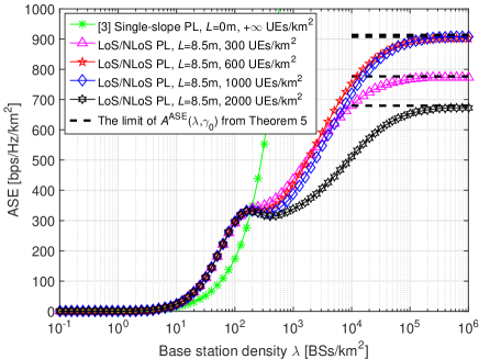
  Fig. 2: The ASE $A^{{\rm{ASE}}}\left(\lambda,\gamma_{0}\right)$ vs. $\lambda$ with $\gamma_{0}=0\,\textrm{dB}$ for the 3GPP Case with $\gamma_{0}=0\,\textrm{dB}$, $L=8.5\,\textrm{m}$ and various values of $\rho$.

VI Conclusion

A constant capacity scaling law has been shown for UDNs. Such law has two profound implications. First, network densification should be stopped at a certain BS density for a given UE density, because the network capacity reaches a limit. Such BS density can be found by solving the BS deployment problem presented in this paper. Second, there exists an optimal SSR density that can maximize the network capacity. In other words, when we deploy thousands or millions of BSs per square kilometer, the best strategy is not activating all BSs on the same time/frequency resource. Such optimal SSR density as well as the corresponding UE density can be found by solving the UE scheduling problem proposed in this paper.

Appendix A: Proof of Theorem 1

As $\lambda\rightarrow+\infty$, we have that $r\rightarrow 0$ and $w\rightarrow L$ in (2). Consequently, the path loss of this link should be dominantly characterized by the first-piece LoS path loss function (i.e., $\zeta_{1}^{{\rm{L}}}\left(w\right)$), which supports the use of $\zeta_{1}^{{\rm{L}}}\left(w\right)$ in such case. Thus, $\underset{\lambda\rightarrow+\infty}{\lim}p^{\textrm{cov}}\left(\lambda,\rho,\gamma\right)$ can be derived as

$$\underset{\lambda\rightarrow+\infty}{\lim}p^{\textrm{cov}}\left(\lambda,\rho,\gamma\right) = \underset{\lambda\rightarrow+\infty}{\lim}{\rm{Pr}}\left[\mathrm{SINR}>\gamma\left|\zeta\left(w\right)=\zeta_{1}^{{\rm{L}}}\left(L\right)\right.\right]$$ (18)

$$\overset{(a)}{=} \underset{\lambda\rightarrow+\infty}{\lim}{\rm{Pr}}\left[\frac{P\zeta_{1}^{{\rm{L}}}\left(L\right)h}{I_{{\rm{agg}}}+P_{{\rm{N}}}}>\gamma\right]$$

$$= \underset{\lambda\rightarrow+\infty}{\lim}{\rm{Pr}}\left[h>\frac{\left(I_{{\rm{agg}}}+P_{{\rm{N}}}\right)\gamma}{P\zeta_{1}^{{\rm{L}}}\left(L\right)}\right],$$

where (6) is plugged into the step (a) of (18). Considering that the complementary cumulative distribution function (CCDF) of $h$ gives ${\rm{Pr}}\left[h>x_{1}+x_{2}\right]=\exp\left(-x_{1}\right)\exp\left(-x_{2}\right)$ and with some mathematical manipulations, we can arrive at (8).

Then, we can further derive $\mathscr{L}_{I_{{\rm{agg}}}}^{{\rm{L}}}\left(s\right)$ with $s=\frac{\gamma}{P\zeta_{1}^{{\rm{L}}}\left(L\right)}$ as

$\mathscr{L}_{I_{{\rm{agg}}}}^{{\rm{L}}}\left(s\right)$

$$= \mathbb{E}_{\left[I_{{\rm{agg}}}\right]}\left\{\exp\left(-sI_{{\rm{agg}}}\right)\right\}$$ (19)

$$\overset{(a)}{=} \mathbb{E}_{\left[\tilde{\Phi}\setminus b_{o},\left\{\beta_{i}\right\},\left\{g_{i}\right\}\right]}\left\{\exp\left(-s\sum_{i\in\Phi/b_{o}}P\beta_{i}g_{i}\right)\right\}$$

$$\overset{(b)}{=} \exp\left(-2\pi\tilde{\lambda}\int_{0}^{\infty}\left(1-\mathbb{E}_{\left[g\right]}\left\{\exp\left(-sP\beta\left(\sqrt{u^{2}+L^{2}}\right)g\right)\right\}\right)udu\right)$$

$$\overset{(c)}{=} \exp\left(-2\pi\tilde{\lambda}\int_{0}^{+\infty}\frac{{\rm{Pr}}^{{\rm{L}}}\left(\sqrt{u^{2}+L^{2}}\right)u}{1+\left(sP\zeta^{{\rm{L}}}\left(\sqrt{u^{2}+L^{2}}\right)\right)^{-1}}du\right)$$

$$\times\exp\left(-2\pi\tilde{\lambda}\int_{0}^{+\infty}\frac{\left[1-{\rm{Pr}}^{{\rm{L}}}\left(\sqrt{u^{2}+L^{2}}\right)\right]u}{1+\left(sP\zeta^{{\rm{NL}}}\left(\sqrt{u^{2}+L^{2}}\right)\right)^{-1}}du\right),$$

where the step (a) of (19) comes from (7), the step (b) of (19) is obtained from Campbell’s theorem [3], and $\mathbb{E}_{\left[g\right]}\left\{\exp\left(-sxg\right)\right\}=\frac{1}{1+sx}$ is plugged into the step (c) of (19) and the aggregate interference from both LoS and NLoS paths are considered therein. Finally, from (1), we have that $\underset{\lambda\rightarrow+\infty}{\lim}\tilde{\lambda}=\rho$, which yields the result of $\underset{\lambda\rightarrow+\infty}{\lim}\mathscr{L}_{I_{{\rm{agg}}}}^{{\rm{L}}}\left(\frac{\gamma}{P\zeta_{1}^{{\rm{L}}}\left(L\right)}\right)$ in (9) and thus concludes our proof.

Appendix B: Proof of Theorem 1

Due to the page limit, here we only provide the key steps of the proof. The proof is mainly consisted of two parts, where (i) in (8), $\exp\left(-\frac{P_{{\rm{N}}}\gamma}{P\zeta_{1}^{{\rm{L}}}\left(L\right)}\right)$ is a function of $L$ and $\gamma$. Note that in reality it is a value very close to 1 because usually we have $P\zeta_{1}^{{\rm{L}}}\left(L\right)\gg P_{{\rm{N}}}$, and (ii) in (9), $\underset{\lambda\rightarrow+\infty}{\lim}\mathscr{L}_{I_{{\rm{agg}}}}^{{\rm{L}}}\left(\frac{\gamma}{P\zeta_{1}^{{\rm{L}}}\left(L\right)}\right)$ is a function of $L$, $\rho$ and $\gamma$.

Appendix C: Proof of Lemma 3

Due to the page limit, here we only provide the key steps of the proof. The proof is mainly consisted of two parts, where for a given $\left\{\rho,\gamma\right\}$, (i) in (8), we have that $\exp\left(-\frac{P_{{\rm{N}}}\gamma}{P\zeta_{1}^{{\rm{L}}}\left(L\right)}\right)$ decreases as $L$ increases, and (ii) in (9), we have that $s=\frac{\gamma}{P\zeta_{1}^{{\rm{L}}}\left(L\right)}$ increases as $L$ increases, and $L$ quickly becomes irrelevant in the integrals of (9) because $L$ appears in the term $\sqrt{u^{2}+L^{2}}$ and the integrals are performed on $u$ toward $u=+\infty$, which leads to the conclusion that $\underset{\lambda\rightarrow+\infty}{\lim}\mathscr{L}_{I_{{\rm{agg}}}}^{{\rm{L}}}\left(s\right)$ is a decreasing function of $s$, and thus $L$.

Appendix D: Proof of Lemma 4

Due to the page limit, here we only provide the key steps of the proof. First, from (9) we conclude that $\exp\left(-\frac{P_{{\rm{N}}}\gamma}{P\zeta_{1}^{{\rm{L}}}\left(L\right)}\right)$$\approx 1$ because usually we have $P\zeta_{1}^{{\rm{L}}}\left(L\right)\gg P_{{\rm{N}}}$ in an interference-limited UDN. Second, the rest of the proof is apparent from the results in Theorem 1.

Appendix E: Proof of Theorem 5

Due to the page limit, here we only provide the key steps of the proof. As $\lambda\rightarrow+\infty$, the ASE in (14) approaches a limit that is independent of $\lambda$. This is because (i) from Theorem 1, we can get that both $\underset{\lambda\rightarrow+\infty}{\lim}p^{\textrm{cov}}\left(\lambda,\rho,\gamma\right)$ and $\underset{\lambda\rightarrow+\infty}{\lim}p^{{\rm{cov}}}\left(\lambda,\rho,\gamma_{0}\right)$ are independent of $\lambda$, and (ii) from (1) we have that $\underset{\lambda\rightarrow+\infty}{\lim}\tilde{\lambda}=\rho$, which is also independent of $\lambda$ and has been plugged into (15). Therefore, $\underset{\lambda\rightarrow+\infty}{\lim}A^{{\rm{ASE}}}\left(\lambda,\rho,\gamma_{0}\right)$ is independent of $\lambda$ as $\lambda\rightarrow+\infty$, which completes our proof.

References

- [1] W. Webb, Wireless Communications: The Future. John Wiley & Sons Ltd., 2007.
- [2] D. L pez-P rez, M. Ding, H. Claussen, and A. Jafari, “Towards 1 Gbps/UE in cellular systems: Understanding ultra-dense small cell deployments,” IEEE Communications Surveys Tutorials, vol. 17, no. 4, pp. 2078–2101, Jun. 2015.
- [3] J. Andrews, F. Baccelli, and R. Ganti, “A tractable approach to coverage and rate in cellular networks,” IEEE Transactions on Communications, vol. 59, no. 11, pp. 3122–3134, Nov. 2011.
- [4] S. Lee and K. Huang, “Coverage and economy of cellular networks with many base stations,” IEEE Communications Letters, vol. 16, no. 7, pp. 1038–1040, Jul. 2012.
- [5] X. Zhang and J. Andrews, “Downlink cellular network analysis with multi-slope path loss models,” IEEE Transactions on Communications, vol. 63, no. 5, pp. 1881–1894, May 2015.
- [6] T. Bai and R. Heath, “Coverage and rate analysis for millimeter-wave cellular networks,” IEEE Transactions on Wireless Communications, vol. 14, no. 2, pp. 1100–1114, Feb. 2015.
- [7] M. Ding, P. Wang, D. L pez-P rez, G. Mao, and Z. Lin, “Performance impact of LoS and NLoS transmissions in dense cellular networks,” IEEE Transactions on Wireless Communications, vol. 15, no. 3, pp. 2365–2380, Mar. 2016.
- [8] M. D. Renzo, W. Lu, and P. Guan, “The intensity matching approach: A tractable stochastic geometry approximation to system-level analysis of cellular networks,” IEEE Transactions on Wireless Communications, vol. 15, no. 9, pp. 5963–5983, Sep. 2016.
- [9] M. Ding and L pez-P rez, “Performance impact of base station antenna heights in dense cellular networks,” to appear in IEEE Transactions on Wireless Communications, arXiv:1704.05125 [cs.NI], Sep. 2017. [Online]. Available: https://arxiv.org/abs/1704.05125
- [10] M. Ding, D. L pez-P rez, G. Mao, and Z. Lin, “Performance impact of idle mode capability on dense small cell networks with LoS and NLoS transmissions,” to appear in IEEE Transactions on Vehicular Technology, arXiv:1609.07710 [cs.NI], Sep. 2017.
- [11] 3GPP, “TR 36.828: Further enhancements to LTE Time Division Duplex for Downlink-Uplink interference management and traffic adaptation,” Jun. 2012.
- [12] M. Ding and D. L pez-P rez, “On the performance of practical ultra-dense networks: The major and minor factors,” The IEEE Workshop on Spatial Stochastic Models for Wireless Networks (SpaSWiN) 2017, pp. 1–8, May 2017.
- [13] I. Atzeni, J. Arnau, and M. Kountouris, “Performance analysis of ultra-dense networks with elevated base stations,” arXiv:1703.06069 [cs.IT], Mar. 2017. [Online]. Available: http://arxiv.org/abs/1703.06069