Spectral approximation of fractional PDEs in image processing and phase field modeling

Abstract

Fractional differential operators provide an attractive mathematical tool to model effects with limited regularity properties. Particular examples are image processing and phase field models in which jumps across lower dimensional subsets and sharp transitions across interfaces are of interest. The numerical solution of corresponding model problems via a spectral method is analyzed. Its efficiency and features of the model problems are illustrated by numerical experiments.

AMS subject classification 35S15, 26A33, 65R20, 65N12, 65N35, 49M05, 49K20

1 Introduction

Let $\mathbb{T}^{d}$, $d\geq 1$, be the $d$-dimensional torus. The purpose of this paper is to study the approximation of problems involving the fractional Laplace operator of order $2s$

$$(-\Delta)^{s}\equiv(-\Delta_{\mathbb{T}^{d}})^{s}$$

using the Fourier spectral method and to illustrate the importance of fractional differential operators. Such operators appear in various models with periodic boundary conditions, see [18, 28, 32]. The approach discussed here extends to problems with other boundary conditions such as Dirichlet or Neumann boundary conditions. For a discussion on nonhomogeneous boundary conditions we refer to [2].

Motivated by applications including fracture mechanics and turbulence, see [24, 16, 21], problems with fractional derivatives have recently gained a lot of interest. Several experiments suggest the presence of fractional derivatives, for instance, the electrical signal propagation in a cardiac tissue [10]. The appearance of fractional derivatives there is attributed to the heterogeneity of the underlying medium. A question arises: can one, for example, tailor the diffusion coefficient in [10] to get the same effects as the fractional model? Indeed to arrive at a direct evidence justifying the presence of fractional derivatives is a difficult question to address. This paper is an attempt to partially address this question by considering two specific applications where the presence of spectral fractional operators makes a significant difference. In particular, we illustrate the effect and advantages of fractional derivatives on two, by now, classical problems: image denoising and phase field modeling.

A well-known total variation based image denoising model is the so-called Rudin–Osher–Fatemi (ROF) model [33] which seeks a minimizer $u\in BV(\mathbb{T}^{d})\cap L^{2}(\mathbb{T}^{d})$ for

$$E(u)=|Du|(\mathbb{T}^{d})+\frac{\alpha}{2}\|u-g\|^{2}.$$ (1.1)

Here $\mathbb{T}^{d}$ denotes the image domain, $\|\cdot\|$ is the norm in $L^{2}(\mathbb{T}^{d};\mathbb{C})$ with corresponding inner product $(\cdot,\cdot)$, and $\alpha>0$ is a regularization parameter. The function $g\mathrel{\mathop{\mathchar 58\relax}}\mathbb{T}^{d}\rightarrow\mathbb{C}$ represents the given observed possibly noisy image. The first term in $E$ is the total variation $|Du|(\mathbb{T}^{d})$ which has a regularizing effect but at the same time allows for discontinuities which may represent edges in the image. The second term is the fidelity term which measures the distance to the given image. Often, weaker norms such as the $H^{-1}$ norm are considered to define the latter term. While the existence and uniqueness of a minimizer can be established via the direct method of calculus of variations, the non-differentiability of the total variation is challenging from a computational point of view. In fact, a non-exhaustive list of papers that have attempted to resolve this are [5, 7, 15, 27, 19, 25, 30, 6]. Another question to ask is, whether natural images belong to $BV(\mathbb{T}^{d})\cap L^{2}(\mathbb{T}^{d})$. The paper [26] shows that natural images are incompletely represented by $BV(\mathbb{T}^{d})$ functions. We will handle both these shortcomings by replacing the total variation term in (1.1) by a squared fractional Sobolev norm. In other words, we propose to minimize

$$E(u)=\frac{1}{2}\|(-\Delta)^{s/2}u\|^{2}+\frac{\alpha}{2}\|(-\Delta)^{-\beta/2}(u-g)\|^{2},$$ (1.2)

with $0<s<1$ and $\beta\in[0,1]$. The first order necessary and sufficient optimality condition determines the unique minimizer $u$ via

$$(-\Delta)^{s}u+\alpha(-\Delta)^{-\beta}(u-g)=0\quad\mbox{in }\mathbb{T}^{d},$$ (1.3)

which is a linear elliptic partial differential equation (PDE) that can be efficiently solved using, for instance, the Fourier spectral method (which is the focus of this paper) or the so-called Caffarelli-Silvestre extension (in $\mathbb{R}^{n}$) [11] and the Stinga-Torrea extension (in bounded domains) [32, 37], see also [31]. Our experiments reveal that the fractional model (1.3) leads to results which are comparable to those provided by the ROF model but at a significantly reduced computational effort (see Section 4). We remark that fractional derivatives have been used in image processing before; see [13, 14], where the authors use spectral methods, and [23], where the authors use the finite element method. However, in both these cases the authors solve a fractional dynamical system with initial condition given by $g$. For completeness, we also refer to [4] where the authors consider a fractional norm equivalent regularization in the context of optimal control problems and parameter identification problems – this equivalent norm was realized using a mutilevel approach.

A mathematical justification of our choice of (1.2) as a substitute to (1.1) is given next. We seek $u$ solving (1.3) in a fractional Sobolev space $H^{s}(\mathbb{T}^{d})$. Moreover, we notice that if $g\in L^{\infty}(\mathbb{T}^{d})$ then following Theorem 3.5 part (1)(b) of [38] it is possible to show that $u\in L^{\infty}(\mathbb{T}^{d})$, see also [3]. We will next see that $BV(\mathbb{T}^{d})\cap L^{\infty}(\mathbb{T}^{d})$ is contained in $H^{s}(\mathbb{T}^{d})$ for $s<1/2$. Indeed by Lemma 38.1 of [39] we have the following continuous embedding

$$BV(\mathbb{T}^{d})\cap L^{\infty}(\mathbb{T}^{d})\subset B^{1/2}_{2,\infty}(\mathbb{T}^{d})$$

where $B^{1/2}_{2,\infty}(\mathbb{T}^{d})$ is a Besov space. In addition, using Proposition 1.2 of [20], see also [29, pg. 1222] and [41, Section 3], we have the following continuous embedding

$$B^{1/2}_{2,\infty}(\mathbb{T}^{d})\subset H^{s}(\mathbb{T}^{d})$$

provided that $s<1/2$. Finally, combining the inclusions we arrive at

$$BV(\mathbb{T}^{d})\cap L^{\infty}(\mathbb{T}^{d})\subset H^{s}(\mathbb{T}^{d}),$$

which justifies our energy functional (1.2). We remark that the regularizing quadratic term in (1.2) does not have the gradient sparsity property of the total variation norm. This effect however cannot be proven for the ROF model in general due the presence of the quadratic fidelity term but is certainly visible in experiments.

As a second example we consider gradient flows of the energy functional

$$E_{\varepsilon}(u)=\frac{1}{2}\|(-\Delta)^{s/2}u\|^{2}+\varepsilon^{-2}\int_{\mathbb{T}^{d}}F(u)\;dx$$ (1.4)

with initial condition $u(0)=u_{0}$. The $L^{2}$-gradient flow of (1.4) leads to the fractional Allen–Cahn equation

$$\begin{aligned} \partial_{t}u+(-\Delta)^{s}u+\varepsilon^{-2}f(u)&=0\;\quad\mbox{in }(0,T)\times\mathbb{T}^{d},\\ u(0,\cdot)&=u_{0}\quad\mbox{in }\mathbb{T}^{d},\end{aligned}$$ (1.5)

where $0<s<1$, $T>0$, and $f=F^{\prime}$ is typically nonlinear in $u$. Moreover,

$$\varepsilon^{-2}\mathrel{\mathop{\mathchar 58\relax}}=\left\{\begin{array}[]{ll}\widetilde{\varepsilon}^{-2s}&\mbox{if }s\in(0,1/2),\\ |\log\widetilde{\varepsilon}|&\mbox{if }s=1/2,\\ \widetilde{\varepsilon}^{1-2s}&\mbox{if }s\in(1/2,1)\end{array}\right.$$

where $0<\widetilde{\varepsilon}<1$. When $s=1$, we set $\varepsilon^{-2}\mathrel{\mathop{\mathchar 58\relax}}=\widetilde{\varepsilon}^{-2}$. The $H^{-\alpha}$ gradient flow, with $\alpha\in(0,1]$ leads to the fractional Cahn–Hilliard equation

$$\begin{aligned} (-\Delta)^{-\alpha}\partial_{t}u+(-\Delta)^{s}u+\varepsilon^{-2}f(u)&=0\quad\;\mbox{in }(0,T)\times\mathbb{T}^{d},\\ u(0,\cdot)&=u_{0}\quad\mbox{in }\mathbb{T}^{d},\end{aligned}$$ (1.6)

By testing (1.6) with a constant function it is easy to check that (1.6) is mass conserving. We note that throughout this article we consider $\widetilde{\varepsilon}$ as a fixed small number. The aforementioned scaling of $\widetilde{\varepsilon}$ is the right scaling to obtain a sharp interface limit as $\widetilde{\varepsilon}\to 0$ we refer the reader to [35]. We remark that even though the optimality system in case of image denoising is linear (1.3), the system for the fractional phase field model is nonlinear (1.6) and controlling these nonlinearities in the presence of fractional derivatives turned out to be a nonobvious task.

When $s=1$, a standard numerical method requires a fine mesh resolution around interfaces to capture sharp transitions [8]. The fully discrete scheme proposed in this paper is unconditionally stable and supported by a rigorous error analysis. In our experiments we observe that using the spectral method and choosing small values for $s$, it is possible to obtain sharp interfaces on relatively coarse meshes and moderate values for $\widetilde{\varepsilon}$.

We remark that the use of spectral methods in the context of phase field models (when $s=1$, $\alpha=0$ or $\alpha=1$) has been considered before, see [9, 17]. We further remark that the recent paper [36] also investigates a fractional Allen–Cahn equation and uses the fractional Riemann-Liouville derivative which is different from our definition. In addition, few analytical details are provided. We also refer to [1] which discusses analytical properties of a fractional Cahn–Hilliard equation with fixed $s=1$. The authors report that the dynamics in case $\alpha>0$ and $s=1$ are closer to the classical Cahn-Hilliard equation than to the Allen-Cahn equation. The error analysis provided there is restricted to spatial discretizations while the used fully discrete scheme treats the nonlinearity explicitly and is hence only conditionally stable.

We remark that the goal of this article is to show possible applications of fractional PDEs. The simple image denoising problem serves as a model problem in which the effect of fractional derivatives of different order becomes directly apparent. The nonlinear evolution model defined by the fractional phase field equation combines different effects so that an interpretation of the effect of fractional derivatives of different order requires a more careful interpretation. Our experiments are meant to illustrate these effects for different parameters $s$.

This paper is organized as follows: In Section 2 we recall facts about spectral interpolation estimates in fractional Sobolev spaces. The fractional Laplace operator and its discretization by the spectral method are addressed in Section 3. We present the details on the fractional image denoising problem in Section 4. Section 5 is devoted to a general error analysis for a numerical scheme covering both the fractional Allen–Cahn and Cahn–Hilliard equations. We conclude with several illustrative numerical examples in Section 6.

2 Spectral approximation

In this section we specify notation needed to define the discrete Fourier transformation and recall elementary approximation results in fractional Sobolev spaces.

2.1 Discrete Fourier transformation

We consider the $2\pi$-periodic torus $\mathbb{T}^{d}$ and the set of grid points $(x_{j}\mathrel{\mathop{\mathchar 58\relax}}j\in\mathbb{N}_{n}^{d})$ on $\mathbb{T}^{d}$ defined by $x_{j}=(j_{1},\dots,j_{d})\frac{2\pi}{n},$ where $\mathbb{N}_{n}^{d}=\big{\{}j=(j_{1},\dots,j_{d})\in\mathbb{Z}^{d}\mathrel{\mathop{\mathchar 58\relax}}0\leq j_{i}\leq n-1\big{\}}.$ A family of grid functions $(\Phi^{k}\mathrel{\mathop{\mathchar 58\relax}}k\in\mathbb{Z}_{n}^{d})$ is defined by

$$\Phi^{k}=\big{(}e^{{\mathrm{i}k\cdot x}_{j}}\mathrel{\mathop{\mathchar 58\relax}}j\in\mathbb{N}_{n}^{d}\big{)},$$

where $\mathbb{Z}_{n}^{d}=\big{\{}k=(k_{1},\dots,k_{d})\in\mathbb{Z}^{d}\mathrel{\mathop{\mathchar 58\relax}}-n/2\leq k_{i}\leq n/2-1\big{\}}$ and $\mathrm{i}^{2}=-1$. For grid functions $V=(v_{j}\mathrel{\mathop{\mathchar 58\relax}}j\in\mathbb{N}_{n}^{d})$ and $W=(w_{j}\mathrel{\mathop{\mathchar 58\relax}}j\in\mathbb{N}_{n}^{d})$ we define the discrete scalar product

$$(V,W)_{n}=\frac{(2\pi)^{d}}{n^{d}}\sum_{j\in\mathbb{N}_{n}^{d}}v_{j}\overline{w}_{j}.$$

The associated norm is denoted $\|\cdot\|_{n}$. Notice that the family $(\Phi^{k}\mathrel{\mathop{\mathchar 58\relax}}k\in\mathbb{Z}_{n}^{d})$ defines an orthogonal basis for the space of grid functions with $\|\Phi^{k}\|_{n}=(2\pi)^{d/2}$. The discrete Fourier transform of a grid function $V=(v_{j}\mathrel{\mathop{\mathchar 58\relax}}j\in\mathbb{N}_{n}^{d})$ is the coefficient vector $\widetilde{V}=(\widetilde{v}_{k}\mathrel{\mathop{\mathchar 58\relax}}{k\in\mathbb{Z}_{n}^{d}})$ with

$$\widetilde{v}_{k}=(V,\Phi^{k})_{n}.$$

With these coefficients we have $V=(2\pi)^{-d}\sum_{k\in\mathbb{Z}_{n}^{d}}\widetilde{v}_{k}\Phi^{k}.$

2.2 Trigonometric interpolation

We consider the space of trigonometric polynomials defined via

$$\mathcal{S}_{n}=\big{\{}v_{n}\in C(\mathbb{T}^{d};\mathbb{C})\mathrel{\mathop{\mathchar 58\relax}}v_{n}(x)=\sum_{k\in\mathbb{Z}_{n}^{d}}c_{k}\varphi^{k}(x),\,c_{k}\in\mathbb{C}\big{\}},$$

with the functions $\varphi^{k}(x)=e^{\mathrm{i}k\cdot x}$ which define an orthogonal basis for $\mathcal{S}_{n}$ with respect to the inner product in $L^{2}(\mathbb{T}^{d};\mathbb{C})$. With $v\in C(\mathbb{T}^{d};\mathbb{C})$ we associate a grid function $V=(v_{j}\mathrel{\mathop{\mathchar 58\relax}}{j\in\mathbb{N}_{n}^{d}})$ via $v_{j}=v(x_{j})$, $j\in\mathbb{N}_{n}^{d}$. Notice that for $v_{n},w_{n}\in\mathcal{S}_{n}$ with associated grid functions $V,W$ we have

$$(v_{n},w_{n})=(V,W)_{n}.$$

The discrete Fourier transformation gives rise to a nodal interpolation operator.

Definition 1.

Given $v\in C(\mathbb{T}^{d};\mathbb{C})$ with nodal values $V=(v_{j}\mathrel{\mathop{\mathchar 58\relax}}{j\in\mathbb{N}_{n}^{d}})$ and discrete Fourier coefficients $\widetilde{V}=(\widetilde{v}_{k}\mathrel{\mathop{\mathchar 58\relax}}{k\in\mathbb{Z}_{n}^{d}})$, the trigonometric interpolant $I_{n}v\in\mathcal{S}_{n}$ of $v$ is defined via

$$I_{n}v=\frac{1}{(2\pi)^{d}}\sum_{k\in\mathbb{Z}_{n}^{d}}\widetilde{v}_{k}\varphi^{k}.$$

Remark 2.

(i) Note that $I_{n}v(x_{j})=v(x_{j})$ for all ${j\in\mathbb{N}_{n}^{d}}$.
(ii) We have $\widetilde{v}_{k}=(v,\varphi^{k})_{n}$ for all ${k\in\mathbb{Z}_{n}^{d}}$.
(iii) We have $(I_{n}v,w_{n})_{n}=(v,w_{n})_{n}$ for all $w_{n}\in\mathcal{S}_{n}$ and $v\in C(\mathbb{T}^{d};\mathbb{C})$.

The (continuous) Fourier transform of a function $v\in L^{2}(\mathbb{T}^{d};\mathbb{C})$ is the coefficient vector $\widehat{V}=(\widehat{v}_{k}\mathrel{\mathop{\mathchar 58\relax}}k\in\mathbb{Z}^{d})$ defined by

$$\widehat{v}_{k}=(v,\varphi^{k}).$$

Note that here the $L^{2}$ inner product is used instead of its discrete approximation. With respect to convergence in $L^{2}(\mathbb{T}^{d};\mathbb{C})$ we have that $v=(2\pi)^{-d}\sum_{k\in\mathbb{Z}^{d}}\widehat{v}_{k}\varphi^{k},$ and, in particular, Plancherel’s formula $(v,w)=(2\pi)^{-d}(\widehat{v},\widehat{w})_{\ell^{2}(\mathbb{Z}^{d})}$.

2.3 Approximation in Sobolev spaces

We analyze the approximation properties of the interpolation operator $I_{n}$ in terms of Sobolev norms and with the help of the $L^{2}$ projection onto $\mathcal{S}_{n}$ which is obtained by truncation of the Fourier series of a function.

Definition 3.

The $L^{2}$ projection $P_{n}\mathrel{\mathop{\mathchar 58\relax}}L^{2}(\mathbb{T}^{d};\mathbb{C})\to\mathcal{S}_{n}$ is for $v\in L^{2}(\mathbb{T}^{d};\mathbb{C})$ defined by the condition that for all $w_{n}\in\mathcal{S}_{n}$ we have

$$(P_{n}v,w_{n})=(v,w_{n}).$$

Note that for every $v\in L^{2}(\mathbb{T}^{d};\mathbb{C})$ we have $P_{n}v=\sum_{k\in\mathbb{Z}_{n}^{d}}\widehat{v}_{k}\varphi^{k}$. The following definition is motivated by the fact that $(\widehat{\partial^{\alpha}v})_{k}=\mathrm{i}^{|\alpha|}k^{\alpha}\widehat{v}_{k}$ for every $\alpha\in\mathbb{N}_{0}^{d}$.

Definition 4.

Given $\mu\geq 0$ the Sobolev space $H^{\mu}(\mathbb{T}^{d};\mathbb{C})$ consists of all functions $v\in L^{2}(\mathbb{T}^{d};\mathbb{C})$ with

$$|v|_{\mu}^{2}=\sum_{k\in\mathbb{Z}^{d}}|k|^{2\mu}|\widehat{v}_{k}|^{2}<\infty.$$

Its dual $H^{-\mu}(\mathbb{T}^{d};\mathbb{C})$ consists of all linear functionals $\psi\mathrel{\mathop{\mathchar 58\relax}}H^{\mu}(\mathbb{T}^{d};\mathbb{C})\to\mathbb{C}$ with

$$|\psi|_{-\mu}^{2}=\sum_{k\in\mathbb{Z}^{d}\setminus\{0\}}|k|^{-2\mu}|\widehat{\psi}_{k}|^{2}<\infty,$$

where $\widehat{\psi}_{k}=\psi(\phi_{k})$.

The Sobolev spaces allow us to quantify approximation properties of the operators $P_{n}$ and $I_{n}$. We refer the reader to Chapter 8 in [34] for details.

Lemma 5 (Projection error).

For $\lambda,\mu\in\mathbb{R}$ with $\lambda\leq\mu$ and $v\in H^{\mu}(\mathbb{T}^{d};\mathbb{C})$ we have

$$|v-P_{n}v|_{\lambda}\leq\Big{(}\frac{n}{2}\Big{)}^{-(\mu-\lambda)}|v|_{\mu}.$$

By comparing $P_{n}$ and $I_{n}$ we obtain a trigonometric interpolation estimate. It is shown in Remark 8.3.1 of [34] that the conditions of the following result cannot be improved in general.

Lemma 6 (Interpolation error).

If $\mu>d/2$, $0\leq\lambda\leq\mu$, and $v\in H^{\mu}(\mathbb{T}^{d};\mathbb{C})$ we have

$$|v-I_{n}v|_{\lambda}\leq c_{d,\lambda,\mu}\Big{(}\frac{n}{2}\Big{)}^{-(\mu-\lambda)}|v|_{\mu}$$

with a constant $c_{d,\lambda,\mu}>0$ that is independent of $v$ and $n$.

We conclude the section with an inverse estimate. Particularly, for every function $v_{n}\in\mathcal{S}_{n}$ and $r\geq s$ we have that

$$|v_{n}|_{r}\leq\max_{{k\in\mathbb{Z}_{n}^{d}}}|k|^{r-s}|v_{n}|_{s}\leq\Big{(}\frac{n}{2}\Big{)}^{r-s}|v_{n}|_{s}.$$ (2.1)

3 Fractional Laplace operator

We define subspaces of Sobolev spaces via

$$\accentset{\circ}{H}^{r}(\mathbb{T}^{d};\mathbb{C})=\big{\{}v\in H^{r}(\mathbb{T}^{d};\mathbb{C})\mathrel{\mathop{\mathchar 58\relax}}\widehat{v}_{0}=0\big{\}}.$$

For $r\geq 0$ the subspaces consist of Sobolev functions with vanishing mean. On the subspaces $\accentset{\circ}{H}^{r}(\mathbb{T}^{d};\mathbb{C})$ the corresponding seminorms $|\cdot|_{r}$ are norms.

Definition 7.

For $s,\mu\geq 0$ and $v\in H^{\mu}(\mathbb{T}^{d};\mathbb{C})$ the fractional Laplacian of $v$ is the (generalized) function $(-\Delta)^{s}v\in\accentset{\circ}{H}^{\mu-2s}(\mathbb{T}^{d};\mathbb{C})$ defined by

$$(-\Delta)^{s}v=\frac{1}{(2\pi)^{d}}\sum_{k\in\mathbb{Z}^{d}{\setminus\{0\}}}|k|^{2s}\widehat{v}_{k}\varphi^{k}.$$

Given $f\in L^{2}(\mathbb{T}^{d};\mathbb{C})$ with vanishing mean the fractional Poisson problem seeks $u\in\accentset{\circ}{H}^{s}(\mathbb{T}^{d};\mathbb{C})$ with

$$(-\Delta)^{s}u=f.$$ (3.1)

The unique solution to (3.1) is given by

$$u=\frac{1}{(2\pi)^{d}}\sum_{k\in\mathbb{Z}^{d}{\setminus\{0\}}}|k|^{-2s}\widehat{f}_{k}\varphi^{k},$$ (3.2)

and in fact satisfies $u\in\accentset{\circ}{H}^{2s}(\mathbb{T}^{d};\mathbb{C})$. More generally, for $f\in\accentset{\circ}{H}^{\mu}(\mathbb{T}^{d};\mathbb{C})$ we have

$$|u|_{\mu+2s}=|f|_{\mu},$$

i.e., the fractional Laplacian defines an isometric isomorphism

$$(-\Delta)^{s}\mathrel{\mathop{\mathchar 58\relax}}\accentset{\circ}{H}^{r}(\mathbb{T}^{d};\mathbb{C})\to\accentset{\circ}{H}^{r-2s}(\mathbb{T}^{d};\mathbb{C}).$$

We define the fractional Laplace operator of negative order as the inverse of $(-\Delta)^{s}$, i.e.,

$$(-\Delta)^{-s}=\big{(}(-\Delta)^{s}\big{)}^{-1}\mathrel{\mathop{\mathchar 58\relax}}\accentset{\circ}{H}^{r}(\mathbb{T}^{d};\mathbb{C})\to\accentset{\circ}{H}^{r+2s}(\mathbb{T}^{d};\mathbb{C}).$$

Note that for $r,s\in\mathbb{R}$ and $v\in\accentset{\circ}{H}^{r}(\mathbb{T}^{d};\mathbb{C})$ with $(-\Delta)^{s}v\in L^{2}(\mathbb{T}^{d};\mathbb{C})$ we have

$$|v|_{s}=\|(-\Delta)^{s/2}v\|.$$

If $s\leq r$ we have the continuous embedding property

$$|v|_{s}\leq|v|_{r}.$$ (3.3)

The discretized fractional Poisson problem seeks for a given $f_{n}\in\mathcal{S}_{n}$ with vanishing mean a function $u_{n}\in\mathcal{S}_{n}$ with

$$(-\Delta)^{s}u_{n}=f_{n}.$$ (3.4)

The uniquely defined solution is given by

$$u_{n}=\frac{1}{(2\pi)^{d}}\sum_{{k\in\mathbb{Z}_{n}^{d}}{\setminus\{0\}}}|k|^{-2s}\widetilde{f}_{k}\varphi^{k}.$$ (3.5)

There are two noticeable differences between the continuous (3.2) and the discrete solutions (3.5). Besides the finite and the infinite sums, $u_{n}$ contains the discrete Fourier coefficients $\widetilde{f}_{k}$ and $u$ contains the continuous Fourier coefficients $\widehat{f}_{k}$. The following a priori error estimates hold.

Theorem 8.

Let $u$ and $u_{n}$ solve the continuous (3.1) and the discrete (3.4) problems, respectively. We have

$$|u-u_{n}|_{s}\leq|f-f_{n}|_{-s}.$$

In particular, if $f\in\accentset{\circ}{H}^{\mu}(\mathbb{T}^{d};\mathbb{C})$ and $f_{n}=P_{n}f$ we have

$$|u-u_{n}|_{s}\leq\Big{(}\frac{n}{2}\Big{)}^{-(\mu+s)}|f|_{\mu},$$

while if $f\in\accentset{\circ}{H}^{\nu}(\mathbb{T}^{d};\mathbb{C})$ with $\nu>d/2$ and $f_{n}=I_{n}f$ we have

$$|u-u_{n}|_{s}\leq c_{d,0,\nu}\Big{(}\frac{n}{2}\Big{)}^{-\nu}|f|_{\nu}.$$

Proof.

In view of (3.1) and (3.4) we have

$$|u-u_{n}|_{s}^{2} =\big{(}(-\Delta)^{s}(u-u_{n}),u-u_{n}\big{)}$$

$$=\big{(}f-f_{n},u-u_{n}\big{)}$$

$$\leq|f-f_{n}|_{-s}|u-u_{n}|_{s}.$$

This implies the general estimate and in combination with Lemma 5 the estimate in case $f_{n}=P_{n}f$. With (3.3) and Lemma 6 we deduce that

$$|f-I_{n}f|_{-s}\leq\|f-I_{n}f\|\leq c_{d,0,\nu}\Big{(}\frac{n}{2}\Big{)}^{-\nu}|f|_{\nu}$$

which implies the estimate. ∎

4 Fractional image denoising

Our second problem is a replacement of the ROF image denoising model (1.1). Given an image $g\in L^{2}(\mathbb{T}^{d};\mathbb{C})$ we propose to minimize

$$E(u)=\frac{1}{2}\|(-\Delta)^{s/2}u\|^{2}+\frac{\alpha}{2}\|(-\Delta)^{-\beta/2}(u-g)\|^{2},$$ (4.1)

with $0<s<1$ and $\beta\in[0,1]$. The minimization is carried out over $H^{s}(\mathbb{T}^{d};\mathbb{C})$ when $\beta=0$ and over $\accentset{\circ}{H}^{s}(\mathbb{T}^{d};\mathbb{C})$ when $\beta$ is positive. In the latter case we assume that $g$ has a vanishing mean. The existence and uniqueness of a minimizer follows by using the direct method in the calculus of variations. The first order necessary and sufficient optimality condition determines the unique minimizer $u$ via

$$(-\Delta)^{s}u+\alpha(-\Delta)^{-\beta}u=\alpha(-\Delta)^{-\beta}g\quad\mbox{in }\mathbb{T}^{d}.$$ (4.2)

We note that since $g\in L^{2}(\mathbb{T}^{d};\mathbb{C})$, we have $u\in H^{2(s+\beta)}(\mathbb{T}^{d};\mathbb{C})$. In particular, the solution to (4.2) is

$$u=\frac{\alpha}{(2\pi)^{d}}\sum_{k\in\mathbb{Z}^{d}}\big{(}|k|^{2(s+\beta)}+\alpha\big{)}^{-1}\widehat{g}_{k}\varphi^{k}.$$

The discretized problem seeks for a given $g_{n}\in\mathcal{S}_{n}$ a function $u_{n}\in\mathcal{S}_{n}$ with

$$(-\Delta)^{s}u_{n}+\alpha(-\Delta)^{-\beta}u_{n}=\alpha(-\Delta)^{-\beta}g_{n}.$$ (4.3)

The uniquely defined solution is given by

$$u_{n}=\frac{\alpha}{(2\pi)^{d}}\sum_{{k\in\mathbb{Z}_{n}^{d}}}\big{(}|k|^{2(s+\beta)}+\alpha\big{)}^{-1}\widetilde{g}_{k}\varphi^{k}$$

Theorem 9.

Let $u$ and $u_{n}$ solve the continuous and the discrete problems (4.3) and (4.2), respectively. We have that

$$|u-u_{n}|_{s}^{2}+\frac{\alpha}{2}|u-u_{n}|_{-\beta}^{2}\leq\frac{\alpha}{2}|g-g_{n}|_{-\beta}^{2}.$$

In particular, if $g\in H^{\mu}(\mathbb{T}^{d};\mathbb{C})$ and $g_{n}=P_{n}g$ we have

$$|u-u_{n}|_{s}+(\alpha/2)^{1/2}|u-u_{n}|_{-\beta}\leq\alpha^{1/2}\Big{(}\frac{n}{2}\Big{)}^{-(\mu+\beta)}|g|_{\mu},$$

while if $g\in H^{\nu}(\mathbb{T}^{d};\mathbb{C})$ with $\nu>d/2$ and $g_{n}=I_{n}g$ we have

$$|u-u_{n}|_{s}+(\alpha/2)^{1/2}|u-u_{n}|_{-\beta}\leq\alpha^{1/2}c_{d,0,\nu}\Big{(}\frac{n}{2}\Big{)}^{-\nu}|g|_{\nu}.$$

Proof.

Testing the difference of (4.2) and (4.3) by $u-u_{n}$ implies that

$$\begin{split}|u-u_{n}|_{s}^{2}+\alpha|u-u_{n}|_{-\beta}^{2}&=\alpha\big{(}(-\Delta)^{-\beta}(g-g_{n}),u-u_{n}\big{)}\\ &\leq\frac{\alpha}{2}|g-g_{n}|_{-\beta}^{2}+\frac{\alpha}{2}|u-u_{n}|_{-\beta}^{2}.\end{split}$$

The estimates follow from using $(a+b)^{2}\leq 2(a^{2}+b^{2})$ and arguing as in the proof of Theorem 8. ∎

5 Fractional phase field equations

Given parameters $\alpha,s\geq 0$ we recall the fractional Cahn-Hilliard equation (1.6)

$$(-\Delta)^{-\alpha}\partial_{t}u+(-\Delta)^{s}u=-\varepsilon^{-2}f(u)$$ (5.1)

on a $d$-dimensional torus $\mathbb{T}^{d}$ and with initial condition $u(0)=u_{0}$. We recall that $\alpha=0$ gives rise to the fractional Allen–Cahn equation (1.5). Below we will impose the restrictions $s>0$ and $s\geq\alpha$.

We assume a splitting of the nonnegative potential $F$ into convex and concave parts $F^{cx}$ and $F^{cv}$ which induces a decomposition of $f=F^{\prime}$ into a monotone and an antimonotone part

$$f=f^{cx}+f^{cv}.$$

We assume for simplicity that $f^{cx}$ and $f^{cv}$ are smooth and Lipschitz continuous. The latter condition is justified by a maximum principle in the case for the Allen–Cahn equation and $L^{\infty}$ bounds for solutions of the Cahn–Hilliard equation [12] corresponding to $(\alpha,s)=(0,1)$ and $(\alpha,s)=(1,1)$, respectively.

5.1 Numerical scheme and error analysis

The numerical scheme computes iterates $(u_{n}^{k})_{k=0,\dots,K}\subset\mathcal{S}_{n}$ via

$$(-\Delta)^{-\alpha}d_{t}u_{n}^{k}+(-\Delta)^{s}u_{n}^{k}+\varepsilon^{-2}I_{n}f^{cx}(u_{n}^{k})=-\varepsilon^{-2}I_{n}f^{cv}(u_{n}^{k-1}).$$ (5.2)

where $d_{t}w^{k}=(w^{k}-w^{k-1})/\tau$ with $\tau>0$ being the time step-size and $u_{n}^{0}$ is a suitable approximation of $u^{0}$. By applying the operator $(-\Delta)^{\alpha}$ and testing the resulting identity with constant functions we observe the mass conservation property $(d_{t}u_{n}^{k},1)=0$ if $\alpha>0$. Existence of the iterates is established via convex minimization problems; if the convex part of $F$ is quadratic then $f^{cx}$ is linear and the scheme (5.2) defines a linear system of equations. The scheme is unconditionally energy stable in the sense that we have

$$|d_{t}u_{n}^{k}|_{-\alpha}^{2}+\frac{\tau}{2}|d_{t}u_{n}^{k}|_{s}^{2}+d_{t}E_{\varepsilon}^{n}(u_{n}^{k})\leq 0,$$

with the discrete energy functional

$$E_{\varepsilon}^{n}(v_{n})=\frac{1}{2}\|(-\Delta)^{s/2}v_{n}\|^{2}+\varepsilon^{-2}\big{(}F(v_{n}),1\big{)}_{n}.$$

This follows from testing (5.2) with $d_{t}u_{n}^{k}$, using

$$\big{(}(-\Delta)^{s}u_{n}^{k},d_{t}u_{n}^{k}\big{)}=\frac{1}{2}d_{t}\|(-\Delta)^{s/2}u_{n}^{k}\|^{2}+\frac{\tau}{2}\|(-\Delta)^{s/2}d_{t}u_{n}^{k}\|^{2},$$

and noting that as a consequence of convexity and concavity we have

$$\begin{split}\big{(}f^{cx}(u_{n}^{k}),d_{t}u_{n}^{k}\big{)}_{n}&\geq\big{(}d_{t}F^{cx}(u_{n}^{k}),1\big{)}_{n},\\ \big{(}f^{cv}(u_{n}^{k-1}),d_{t}u_{n}^{k}\big{)}_{n}&\geq\big{(}d_{t}F^{cv}(u_{n}^{k}),1\big{)}_{n}.\end{split}$$

Assuming initial data with $E_{\varepsilon}^{n}(u_{n}^{0})\leq c$ as $n\to\infty$, the energy estimate provides a priori bounds on interpolants of the approximations which allows us to select an accumulation point

$$u\in H^{1}([0,T];H^{-\alpha}(\mathbb{T}^{d}))\cap L^{\infty}([0,T];H^{s}(\mathbb{T}^{d}))$$

as $\tau\to 0$ and $n\to\infty$. Its identification as a solution for the fractional Cahn–Hilliard equation follows from the Aubin–Lions lemma provided that $s>0$. Uniqueness of solutions is a consequence of the assumed Lipschitz continuity of $f$. For an error analysis we note that $u\in C([0,T];L^{2}(\mathbb{T}^{d}))$, let $u^{k}=u(t_{k})$ with $t_{k}=k\tau$, and define

$$e_{n}^{k}=u_{n}^{k}-P_{n}u^{k},$$

where $P_{n}$ is the orthogonal projection given in Definition 3. Note that we have $(P_{n}v,w_{n})_{n}=(P_{n}v,w_{n})$ but $(v,w_{n})_{n}\neq(v,w_{n})$ unless $v$ belongs to $\mathcal{S}_{n}$. We omit the subscript $n$ whenever the scalar product is applied to two functions belonging to $\mathcal{S}_{n}$. For ease of readability we abbreviate

$$f_{\varepsilon}=\varepsilon^{-2}f,\quad f_{\varepsilon}^{cx}=\varepsilon^{-2}f^{cx},\quad f_{\varepsilon}^{cv}=\varepsilon^{-2}f^{cv}.$$

The sequences $(u_{n}^{k})$ and $(u^{k})$ satisfy the discrete equations

$$\begin{split}(-\Delta)^{-\alpha}d_{t}u_{n}^{k}+(-\Delta)^{s}u_{n}^{k}&=-I_{n}f_{\varepsilon}(u_{n}^{k})-I_{n}\big{(}f_{\varepsilon}^{cv}(u_{n}^{k-1})-f_{\varepsilon}^{cv}(u_{n}^{k})\big{)},\\ (-\Delta)^{-\alpha}d_{t}P_{n}u^{k}+(-\Delta)^{s}P_{n}u^{k}&=-P_{n}f_{\varepsilon}(u^{k})+(-\Delta)^{-\alpha}P_{n}(d_{t}u^{k}-\partial_{t}u^{k}),\end{split}$$

where we used that $P_{n}$ commutes with $(-\Delta)^{r}$ for every $r\in\mathbb{R}$. Subtracting the identities leads to the error equation

$$(-\Delta)^{-\alpha}d_{t}e_{n}^{k}+(-\Delta)^{s}e_{n}^{k}=A_{n}^{k}+B_{n}^{k}+C_{n}^{k},$$

with the discretization errors

$$\begin{split}A_{n}^{k}&=-I_{n}f_{\varepsilon}(u_{n}^{k})+P_{n}f_{\varepsilon}(u^{k}),\\ B_{n}^{k}&=-I_{n}\big{(}f_{\varepsilon}^{cv}(u_{n}^{k-1})-f_{\varepsilon}^{cv}(u_{n}^{k})\big{)},\\ C_{n}^{k}&=-(-\Delta)^{-\alpha}P_{n}(d_{t}-\partial_{t})u^{k}.\end{split}$$

Testing the error equation with $e_{n}^{k}$ shows that we have

$$\begin{split}\frac{1}{2}d_{t}|e_{n}^{k}|_{-\alpha}^{2}+\frac{\tau}{2}|d_{t}e_{n}^{k}|_{-\alpha}^{2}+|e_{n}^{k}|_{s}^{2}=(A_{n}^{k},e_{n}^{k})+(B_{n}^{k},e_{n}^{k})+(C_{n}^{k},e_{n}^{k}).\end{split}$$

To bound the first term on the right-hand side we insert $f_{\varepsilon}(u_{n}^{k})$, use Lemma 6, the inverse estimate (2.1), and insert $P_{n}u^{k}$ to deduce with the Lipschitz continuity of $f_{\varepsilon}$ that

$$\begin{split}(A_{n}^{k},e_{n}^{k})&=-\big{(}I_{n}f_{\varepsilon}(u_{n}^{k})-f_{\varepsilon}(u_{n}^{k})+f_{\varepsilon}(u_{n}^{k})-f_{\varepsilon}(u^{k}),e_{n}^{k}\big{)}\\ &\leq c_{d,0,1}n^{-1}|f_{\varepsilon}(u_{n}^{k})|_{1}\|e_{n}^{k}\|+|f_{\varepsilon}|_{\text{Lip}}\|u_{n}^{k}-u^{k}\|\|e_{n}^{k}\|\\ &\leq c_{d,0,1}n^{-1}|f_{\varepsilon}|_{\text{Lip}}|u_{n}^{k}|_{1}\|e_{n}^{k}\|+|f_{\varepsilon}|_{\text{Lip}}\big{(}\|u_{n}^{k}-P_{n}u^{k}\|+\|P_{n}u^{k}-u^{k}\|\big{)}\|e_{n}^{k}\|\\ &\leq|f_{\varepsilon}|_{\text{Lip}}\big{(}c_{d,0,1}n^{-s}|u_{n}^{k}|_{s}+\|P_{n}u^{k}-u^{k}\|\big{)}\|e_{n}^{k}\|+|f_{\varepsilon}|_{\text{Lip}}\|e_{n}^{k}\|^{2}.\end{split}$$

For the second term we have that

$$(B_{n}^{k},e_{n}^{k})\leq\tau|f_{\varepsilon}|_{\text{Lip}}\|d_{t}u_{n}^{k}\|\|e_{n}^{k}\|\leq\tau n^{\alpha}|f_{\varepsilon}|_{\text{Lip}}|d_{t}u_{n}^{k}|_{-\alpha}\|e_{n}^{k}\|,$$

where we used the inverse estimate $\|w_{n}\|\leq n^{\alpha}|w_{n}|_{-\alpha}$ if $\alpha>0$. For the third term we assume that $u\in C^{2}([0,T];H^{-\alpha}(\mathbb{T}^{d}))$ and estimate

$$(C_{n}^{k},e_{n}^{k})=((-\Delta)^{-\alpha}[\partial_{t}-d_{t}]u^{k},e_{n}^{k})\leq\frac{\tau}{2}\sup_{t\in[0,T]}|\partial_{t}^{2}u(t)|_{-\alpha}|e_{n}^{k}|_{\alpha}$$

A combination of the estimates, multiplication by $\tau$, and summation over $k=1,2,\dots,K$, yield that

$$\begin{split}&\frac{1}{2}|e_{n}^{K}|_{-\alpha}^{2}+\tau\sum_{k=1}^{K}|e_{n}^{k}|_{s}^{2}\leq\frac{1}{2}|e_{n}^{0}|_{-\alpha}^{2}+K\tau|f_{\varepsilon}|_{\text{Lip}}\max_{k=1,\dots,K}\big{(}c_{d,0,1}n^{-s}|u_{n}^{k}|_{s}+\|u^{k}-P_{n}u^{k}\|\big{)}^{2}\\ &\quad+K\tau^{3}n^{2\alpha}|f_{\varepsilon}|_{\text{Lip}}\max_{k=1,\dots,K}|d_{t}u_{n}^{k}|_{-\alpha}^{2}+K\tau^{3}\sup_{t\in[0,T]}|\partial_{t}^{2}u(t)|_{-\alpha}^{2}\\ &\quad+3|f_{\varepsilon}|_{\text{Lip}}\tau\sum_{k=1}^{K}\|e_{n}^{k}\|^{2}+\frac{\tau}{4}\sum_{k=1}^{K}|e_{n}^{k}|_{\alpha}^{2}.\end{split}$$

If $\alpha=0$ we may directly apply the discrete Gronwall lemma to obtain an error estimate. If $\alpha>0$ we assume $\alpha\leq s$, require that $(u_{n}^{0},1)=(u^{0},1)$ so that $(e_{n}^{k},1)=0$, and use the bound

$$\|e_{n}^{k}\|^{2}\leq|e_{n}^{k}|_{-s}|e_{n}^{k}|_{s}\leq|e_{n}^{k}|_{-\alpha}|e_{n}^{k}|_{s},$$

to deduce with Young’s inequality the estimate

$$E_{n}^{K}=\frac{1}{2}|e_{n}^{K}|_{-\alpha}^{2}+\frac{\tau}{2}\sum_{k=1}^{K}|e_{n}^{k}|_{s}^{2}\leq D_{0}+D_{1}\tau\sum_{k=1}^{K}E_{n}^{k}.$$

Here, $D_{0}$ is the sum of the first four terms on the right-hand side of the above estimate and $D_{1}=2(3|f_{\varepsilon}|_{\text{Lip}})^{2}$. The discrete Gronwall lemma leads to the estimate

$$E_{n}^{K}\leq 2D_{0}\exp(D_{1}T)$$

for all $K$ with $K\tau\leq T$ provided that $\tau D_{1}\leq 1/2$. With the triangle inequality and approximation estimates for $P_{n}$ we obtain the following error estimate.

Theorem 10.

Let $u\in C([0,T];H^{s}(\mathbb{T}^{d}))\cap C^{2}([0,T];H^{-\alpha}(\mathbb{T}^{d}))$ solve (1.6) and let the sequence $(u_{n}^{k})_{k=0,\dots,K}\subset\mathcal{S}_{n}$ be defined via (5.2). There exists a constant $c_{\varepsilon}>0$ such that we have

$$\max_{k=1,\dots,K}|u(t_{k})-u_{n}^{k}|_{-\alpha}\leq c_{\varepsilon}(\tau+\tau n^{\alpha}+n^{-s})$$

for all $\tau>0$ and $n\in\mathbb{N}$.

The constant $c_{\varepsilon}$, in general, depends exponentially on $\varepsilon^{-1}$. For the derivation of this estimate we used the indicated regularity assumption. By standard arguments, see [40] the regularity assumption on the exact solution can be weakened to the conditions

$$u\in L^{\infty}([0,T];H^{s}(\mathbb{T}^{d})),\quad\partial_{t}^{2}u\in L^{2}([0,T];H^{-\alpha}(\mathbb{T}^{d})).$$

The suboptimal term $\tau n^{\alpha}$ corresponds to the semi-implicit treatment of the nonlinearity which makes the scheme (5.2) fully practical.

5.2 Improved error estimate via spectral bounds

A significantly improved error estimate can be obtained if additional analytical knowledge about the evolution is available, e.g., in the form of lower bounds for the principal eigenvalue

$$\lambda(t)=\min_{v\in H^{s}(\mathbb{T}^{d})}\frac{|v|_{s}^{2}+\varepsilon^{-2}\big{(}f^{\prime}(u(t))v,v\big{)}}{|v|_{-\alpha}^{2}}.$$

For ease of presentation we only consider the fractional Allen–Cahn equation with $\alpha=0$ and outline the main arguments following [22, 8]. We focus on the contribution to the error equation resulting from the nonlinearity and write it with abstract consistency functionals $\mathcal{C}_{n}^{k}$ as

$$d_{t}e_{n}^{k}+(-\Delta)^{s}e_{n}^{k}=\mathcal{C}_{n}^{k}+\varepsilon^{-2}P_{n}\big{(}f(u^{k})-f(u_{n}^{k})\big{)}.$$

A precise formula for $\mathcal{C}_{n}^{k}$ is obtained from subtracting the projected partial differential equation evaluated at $t_{k}$ onto $\mathcal{S}_{n}$ from the numerical scheme as above, e.g., in case of a fully implicit numerical scheme with a nodal interpolation of the nonlinear term we have

$$\begin{split}\mathcal{C}_{n}^{k}&=-\varepsilon^{-2}\big{(}P_{n}f(u_{n}^{k})-I_{n}f(u_{n}^{k})\big{)}+\varepsilon^{-2}P_{n}f(u^{k})+d_{t}P_{n}u^{k}+(-\Delta)^{s}P_{n}u^{k}\\ &=-\varepsilon^{-2}\big{(}P_{n}f(u_{n}^{k})-I_{n}f(u_{n}^{k})\big{)}+P_{n}\big{(}d_{t}u^{k}-\partial_{t}u(t_{k})\big{)}.\end{split}$$

To relate the error equation to the principal eigenvalue we require a controlled failure of monotonicity for $f$ in the sense that there exists a constant $c_{f}>0$ such that for all $a,b\in\mathbb{R}$ we have

$$\big{(}f(a)-f(b)\big{)}(a-b)\geq f^{\prime}(a)(a-b)^{2}-c_{f}|a-b|^{3}.$$

With this estimate we deduce with $c_{f}^{\prime}=\|f^{\prime}\|_{L^{\infty}(\mathbb{R})}$ that

$$\begin{split}\frac{1}{2}d_{t}&\|e_{n}^{k}\|^{2}+\frac{\tau}{2}\|d_{t}e^{n}_{k}\|^{2}+|e_{n}^{k}|_{s}^{2}\\ &=-\varepsilon^{-2}\big{(}f(u^{k})-f(u_{n}^{k}),e_{n}^{k}\big{)}+(\mathcal{C}_{n}^{k},e_{n}^{k})\\ &\leq-\varepsilon^{-2}\big{(}f^{\prime}(u^{k})e_{n}^{k},e_{n}^{k}\big{)}+c_{f}\varepsilon^{-2}\|e_{n}^{k}\|_{L^{3}(\mathbb{T}^{d})}^{3}+\frac{\varepsilon^{-2}}{2}|\mathcal{C}_{n}^{k}|_{-s}^{2}+\frac{\varepsilon^{2}}{2}|e_{n}^{k}|_{s}^{2}\\ &\leq-(1-\theta)\varepsilon^{-2}\big{(}f^{\prime}(u^{k})e_{n}^{k},e_{n}^{k}\big{)}+\theta\varepsilon^{-2}c_{f}^{\prime}\|e_{n}^{k}\|^{2}\\ &\qquad+c_{f}\varepsilon^{-2}\|e_{n}^{k}\|_{L^{3}(\mathbb{T}^{d})}^{3}+\frac{\varepsilon^{-2}}{2}|\mathcal{C}_{n}^{k}|_{-s}^{2}+\frac{\varepsilon^{2}}{2}|e_{n}^{k}|_{s}^{2}.\end{split}$$

We incorporate the eigenvalue $\lambda^{k}=\lambda(t_{k})$ via

$$-\varepsilon^{-2}\big{(}f^{\prime}(u^{k})e_{n}^{k},e_{n}^{k}\big{)}\leq|e_{n}^{k}|_{s}^{2}-\lambda^{k}\|e_{n}^{k}\|^{2}.$$

Choosing $\theta=\varepsilon^{2}$ and letting $\mu^{k}=\max\{-\lambda^{k},0\}$ thus leads to the estimate

$$\begin{split}\frac{1}{2}d_{t}\|e_{n}^{k}\|^{2}+|e_{n}^{k}|_{s}^{2}\leq&(1-\varepsilon^{2})|e_{n}^{k}|_{s}^{2}+\mu^{k}\|e_{n}^{k}\|^{2}\\ &+c_{f}^{\prime}\|e_{n}^{k}\|^{2}+c_{f}\varepsilon^{-2}\|e_{n}^{k}\|_{L^{3}(\mathbb{T}^{d})}^{3}+\frac{\varepsilon^{-2}}{2}|\mathcal{C}_{n}^{k}|_{-s}^{2}+\frac{\varepsilon^{2}}{2}|e_{n}^{k}|_{s}^{2}.\end{split}$$

Rearranging terms gives

$$\begin{split}d_{t}&\|e_{n}^{k}\|^{2}+\varepsilon^{2}|e_{n}^{k}|_{s}^{2}\leq 2\big{(}\mu^{k}+c_{f}^{\prime})\|e_{n}^{k}\|^{2}+2c_{f}\varepsilon^{-2}\|e_{n}^{k}\|_{L^{3}(\mathbb{T}^{d})}^{3}+\varepsilon^{-2}|\mathcal{C}_{n}^{k}|_{-s}^{2}.\end{split}$$

In an inductive argument we may assume that $\varepsilon^{-2}\|e_{n}^{k}\|_{L^{3}(\mathbb{T}^{d})}^{3}\leq c\|e_{n}^{k}\|^{2}$ and use the discrete Gronwall lemma to obtain an error estimate that depends exponentially on the principal eigenvalue $\lambda^{k}$. Hence, if $\lambda^{k}$ is uniformly bounded from below the resulting error estimate depends only algebraically on $\varepsilon^{-1}$. More generally, it suffices to assume that a discrete time integral of $\lambda^{k}$ is uniformly bounded from below. This allows us to cover large classes of evolutions including topological changes.

6 Numerical Examples

In this Section, we present several numerical examples. In Section 6.1 we discuss the approximation of the fractional Poisson problem. Section 6.2 is devoted to image denoising problem. In Section 6.3 we study features of the fractional Allen–Cahn equation. We conclude with experiments for the fractional Cahn–Hilliard equation in Section 6.4.

6.1 Approximation of the Poisson problem

To construct a nonsmooth solution for the fractional Poisson problem we first let $w\in C(\mathbb{T})$ be defined via

$$w(x)=\begin{cases}x,&x\leq\pi,\\ 2\pi-x,&x\geq\pi.\end{cases}$$

Since $w(0)=w(2\pi)$ we find for $k\neq 0$ with an integration-by-parts that

$$\widehat{w}_{k}=\int_{0}^{2\pi}w(x)e^{-{\mathrm{i}k\cdot x}}\,{\mathrm{d}}x=\frac{1}{\mathrm{i}k}(1-e^{-\mathrm{i}kx})\int_{0}^{\pi}e^{-{\mathrm{i}k\cdot x}}\,{\mathrm{d}}x=\frac{1}{(\mathrm{i}k)^{2}}\big{(}1-(-1)^{k}\big{)}^{2},$$

i.e., $\widehat{w}_{k}=-4/k^{2}$ if $k$ is odd and $\widehat{w}_{k}=0$ if $k$ is even. We have $\widehat{w}_{0}=\pi^{2}$. We then let $u\in C(\mathbb{T}^{d})$ be for $x\in\mathbb{T}^{d}$ defined via

$$u(x)=\prod_{i=1}^{d}w(x_{i})-\frac{\pi^{2d}}{(2\pi)^{d}}.$$

We have $\widehat{u}_{k}=\widehat{w}_{k_{1}}\cdots\widehat{w}_{k_{d}}$ if $k\neq 0$ and $\widehat{u}_{0}=0$. We set $f=(-\Delta)^{s}u$, i.e., for ${k\in\mathbb{Z}_{n}^{d}}$ let $\widehat{f}_{k}=|k|^{2s}\widehat{u}_{k}$. Note that $f\in L^{2}(\mathbb{T}^{d})$ if and only if $s<1/2$. We choose the approximation $f_{n}=P_{n}f$ which is explicitly available here. The output for $s=1/2$ and $n=16$ is displayed in Figure 1. In contrast to solutions of the classical Poisson problem we observe here the occurrence of kinks in the solution.

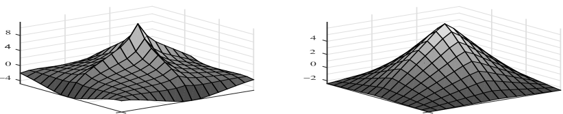
Figure 1: Functions $P_{n}f$ and $u_{n}$ for the fractional Poisson problem with $s=1/2$ and $n=16$.

6.2 Fractional image denoising

The fractional Laplacian with $s<1/2$ is closely related to the total variation norm (see Section 1) which motivates its application in image processing. Given a noisy image $g\in L^{2}(\mathbb{T}^{d})$ we define a regularized image $u\in H^{2s}(\mathbb{T}^{d})$ via

$$(-\Delta)^{s}u+\alpha(u-g)=0.$$

The fidelity parameter $\alpha$ penalizes the deviation of $u$ from $g$ in the $L^{2}$ metric. Alternatively, this distance can be taken in the weaker metric of $H^{-1}(\mathbb{T}^{d})$ which leads to the equation

$$(-\Delta)^{s}u+\alpha(-\Delta)^{-1}(u-g)=0,$$

where we assume that $g$ has vanishing mean and look for $u$ with vanishing mean. The results of two experiments are displayed in the rows of Figure 2. In the first experiment we set $s=0.42$, $\alpha=10$, and $n=1566$. In the second experiment we used $s=0.35$, $\alpha=5\times 10^{3}$ and $n=256$. The first and second columns display the original and noisy images, respectively. The third and fourth columns show the results of $L^{2}$ and $H^{-1}$ fidelity. We note that in the first example, where the additive noise is normally distributed with mean zero and standard deviation $0.15$, the $L^{2}$-fidelity almost perfectly recovers the original image reflecting the fact that for Gaussian noise this is statistically the optimal choice. In the second example where the noise is given by the nodal interpolant of the sinusoidal function

$$\xi(x_{1},x_{2})=5\sin(20\pi x_{1})\sin(20\pi x_{2})$$

we obtain better recovery using the $H^{-1}$-fidelity. We remark that it took 0.2 sec and 0.006 sec to solve the first and the second problem in Matlab on a MacBook Pro with an 2.8 GHz Intel Core i7 processor (16 GB 1600 MHz DDR3 RAM).

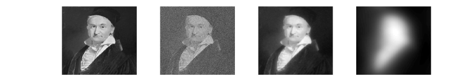
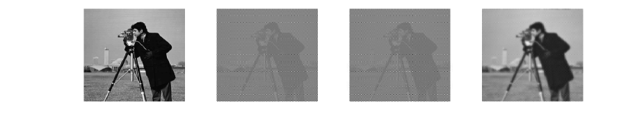
Figure 2: Original and noisy image, regularized images for $L^{2}$ and $H^{-1}$ fidelity terms. In the case of first example we have set $s=0.42$, $\alpha=10$, and $n=1566$. In the second example we have $s=0.35$, $\alpha=5\times 10^{3}$ and $n=256$. The recovery is satisfactory using the $L^{2}$-fidelity in the first example. In the second example, recovery is better in case of the $H^{-1}$-fidelity term.

Comparison between fractional and total variation

We next compare the fractional and the total variation (TV) based models (1.1) with the help of three examples. This comparison was carried out in Python which was specifically chosen due to the availability of SciKit-Image toolbox [42]. In all the examples we assume that original image denoted by $o$ (without noise) is known. For the fractional case we compute the optimal parameters $(s,\alpha)$ by solving a minimization problem: $\min_{u}$ $\|u-o\|^{2}$, subject to $u$ solving $(-\Delta)^{s}u+\alpha(u-g)=0.$ We further assume that $(s,\alpha)$ lies in a closed convex set, i.e., $0.05\leq s\leq 0.5$ and $1\leq\alpha\leq 50$. We solve this optimization problem using an in-built optimization algorithm in Python. The corresponding optimization problem for TV is solved for $\alpha$ using a genetic algorithm.

Our first example uses a picture of Gauss (cf. Figure 3, top row). The left image is the original image with $n=n_{x}=n_{y}=1566$. Our second example (cf. Figure 3, middle row) uses a synthetic image with $n=n_{x}=n_{y}=1500$. Our final example (cf. Figure 3, bottom row) is based on an in-built image from SciKit with different number of points in the $x$ and $y$ directions, i.e., $n_{x}=400$, $n_{y}=600$. We note that even though the approach discussed in Section 4 assumes $n=n_{x}=n_{y}$ it is directly extended to this case where $n_{x}\neq n_{y}$. In the second column (from the left), in all the examples, we have added a normally distributed noise with mean zero and standard deviation $0.15$, we denote the resulting noisy image by $g$.

For the fractional case the optimal parameters are $(s,\alpha)=(0.49,50)$ for the first example and $(s,\alpha)=(0.5,50)$ for the second and third examples. On the other hand, for TV case the optimal parameters are $\alpha=3.58$, $\alpha=1.0$, and $\alpha=8.74$, respectively. Using these parameters we solve the corresponding image denoising problems using the fractional approach (third column from the left) and compare the results with the in-built TV algorithm from [42]. We observe that the two approaches give comparable results in all three examples. The fractional approach is significantly cheaper as only two discrete Fourier transformations have to be computed. The CPU times for implementations of the fractional and TV approach in Matlab and Python, respectively, are provided in the caption of Figure 3. They show a reduction of the computing times by factors 10-100. We remark that certain aspects in the Chambolle–Pock algorithm implemented in Scikit such as the specification of a suitable stopping criterion and choice of step-sizes may lead to different results.

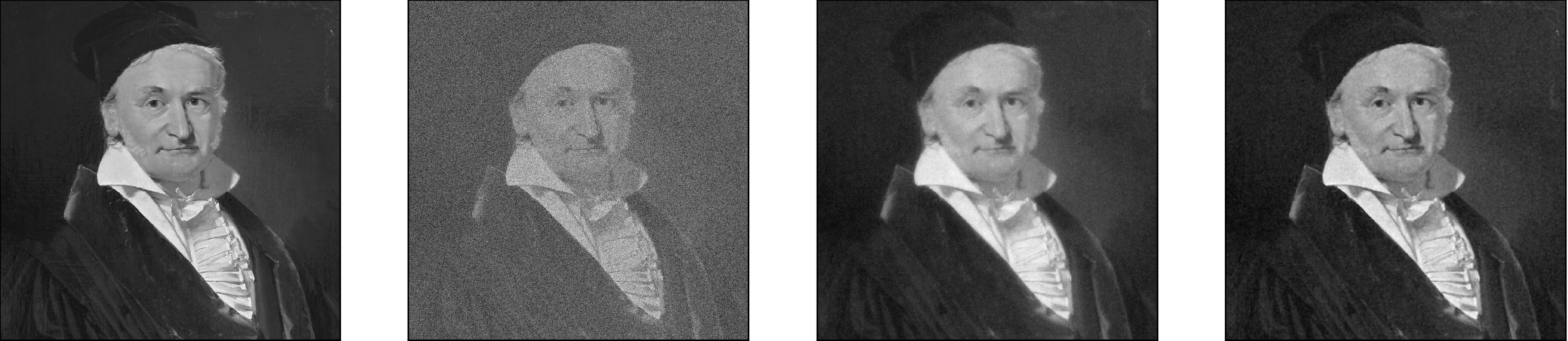
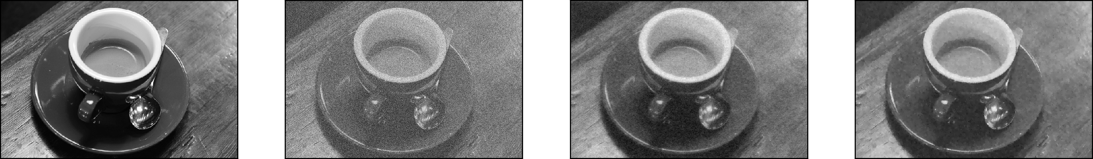
Figure 3: Original and noisy image, regularized images for $L^{2}$ fidelity with fractional and total variation (TV) approaches. The optimized parameters $s$ and $\alpha$ are given as follows - Example 1: $(s,\alpha)=(0.49,50)$ (fractional) and $\alpha=3.58$ (TV); Example 2: $(s,\alpha)=(0.5,50)$ (fractional) and $\alpha=1$ (TV); Example 3: $(s,\alpha)=(0.5,50)$ (fractional) and $\alpha=8.74$ (TV). The last two columns are corresponding reconstructions for the fractional and TV method. While the results are comparable the computing times differ significantly: Example 1: 0.2 sec (fractional) and 2.1 sec (TV); Example 2: 0.1 sec (fractional), 6.1 sec (TV); Example 3: 0.01 sec (fractional) and 0.2 (TV).

6.3 Fractional Allen–Cahn equation

We consider the fractional Allen-Cahn equation (1.5) with a given initial function $u_{0}\in L^{2}(\mathbb{T}^{d})$. The function $f$ is the derivative of a double well potential $F$ with quadratic growth, i.e.,

$$F(u)=\frac{1}{2}\frac{(1-u^{2})^{2}}{1+u^{2}},\quad f(u)=u-\frac{4u}{(1+u^{2})^{2}},$$

which leads to linear systems of equations in our semi-implicit time discretization. Snapshots of the evolutions with $\widetilde{\varepsilon}=1/8$, $n=512$, and $\Delta t=1/100$ at $t=1$, $t=4$, $t=12$, and $t=20$ (rowwise) are shown in Figure 4. The first column corresponds to $s=1$, second to $s=0.45$, third to $s=0.30$, and finally fourth to $s=0.15$. Clearly the interface in case of a fractional model is sharper, however the dynamics are slower.

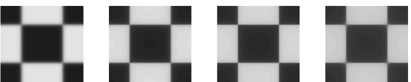
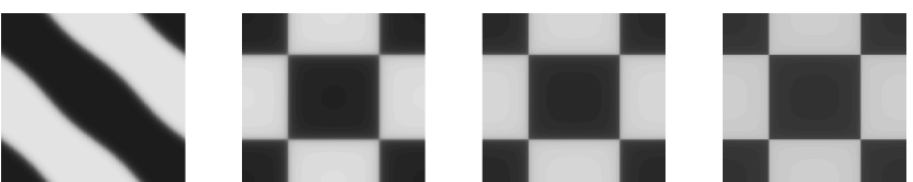
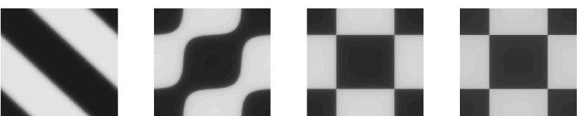
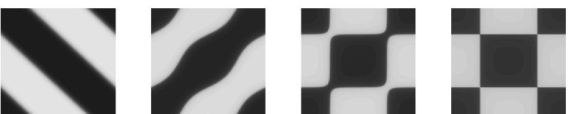
Figure 4: Snapshots of Allen–Cahn evolutions with $n=512$ at times $t=1$, $t=4$, $t=12$, and $t=20$ (rowwise), respectively. Columns represent $s=1$, $s=0.45$, $s=0.30$, and $s=0.15$, respectively. In all cases we have set $\widetilde{\varepsilon}=1/8$.

6.4 Fractional Cahn-Hilliard equation

We next study the fractional Cahn–Hilliard equation specified in (1.6) defining $F$ and $f$ as in Subsection 6.3. In a first experiment we define the initial condition $u_{0}$ as

$$u_{0}(x_{1},x_{2})=\begin{cases}1&\text{if }(x_{1}-\frac{2\pi}{3})^{2}+(x_{2}-\pi)^{2}<(\frac{\pi}{3})^{2}\\ &\mbox{ or }(x_{1}-\frac{4\pi}{3})^{2}+(x_{2}-\pi)^{2}<(\frac{\pi}{3})^{2},\\ -1&\mbox{otherwise}.\end{cases}$$

Snapshots of the evolutions with $\widetilde{\varepsilon}=1/8$, $n=512$, and $\Delta t=1/100$ at $t=0.25$, $t=0.50$, $t=2$, and $t=3$ (rowwise) are shown in Figure 5 for $s=1$, $s=0.45$, $s=0.30$, and $s=0.15$ (columnwise) with $\alpha=1$ in all cases.

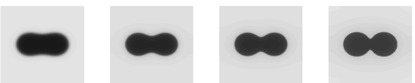
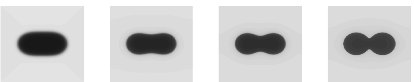
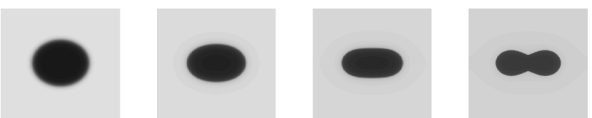
Figure 5: Snapshots of Cahn–Hilliard evolutions with $n=512$ where the rows correspond to $t=0.25$, $t=0.50$, $t=2$, and $t=3$, respectively. Columns represent $s=1$, $s=0.45$, $s=0.30$, and $s=0.15$, respectively. In all cases we have set $\widetilde{\varepsilon}=1/8$ and $\alpha=1$.

In a second experiment we focus on the coarsening dynamics of the fractional phase field equation. As in [1] the initial condition is given by $u_{0}=2\phi-1+\delta$ where $\delta$ is a random perturbation uniformly distributed in [-0.2,0.2]. Snapshots of the evolutions with $\phi=0.5$, $\widetilde{\varepsilon}=1/8$, $n=512$, and $\Delta t=1/100$ at $t=0.25$, $t=0.5$, $t=1$, and $t=1.5$ (rowwise) are shown in Figure 6. The first two columns correspond to $\alpha=1$ with $s=1$ and $s=0.20$, respectively. The last two columns are obtained with $\alpha=1/2$ with $s=1$ and $s=0.20$, respectively.

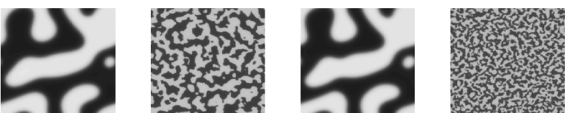
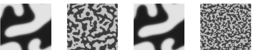
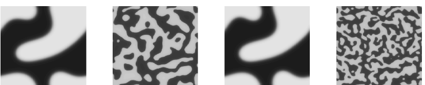
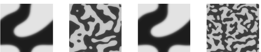
Figure 6: Snapshots of Cahn–Hilliard evolutions at $t=0.25$, $t=0.5$, $t=1$, and $t=1.5$ for $\widetilde{\varepsilon}=1/8$ (rowwise). The first two columns represent $s=1$ and $s=0.20$, respectively with $\alpha=1$. The last two columns correspond to $s=1$ and $s=0.20$, respectively but here $\alpha=1/2$.

Funding

The work of the first author is partially supported by NSF grant DMS-1521590.

References

- [1] M. Ainsworth and Z. Mao. Analysis and Approximation of a Fractional Cahn–Hilliard Equation. SIAM J. Numer. Anal., 55(4):1689–1718, 2017.
- [2] H. Antil, J. Pfefferer, and S. Rogovs. Fractional operators with inhomogeneous boundary conditions: Analysis, control, and discretization. arXiv preprint arXiv:1703.05256, 2017.
- [3] H. Antil, J. Pfefferer, and M. Warma. A note on semilinear fractional elliptic equation: analysis and discretization. To appear: ESAIM: M2AN, 2017.
- [4] U. Aßmann and A. Rösch. Regularization in Sobolev spaces with fractional order. Numer. Funct. Anal. Optim., 36(3):271–286, 2015.
- [5] S. Bartels. Total variation minimization with finite elements: convergence and iterative solution. SIAM J. Numer. Anal., 50(3):1162–1180, 2012.
- [6] S. Bartels. Numerical methods for nonlinear partial differential equations, volume 47 of Springer Series in Computational Mathematics. Springer, Cham, 2015.
- [7] S. Bartels. Broken Sobolev space iteration for total variation regularized minimization problems. IMA J. Numer. Anal., 36(2):493–502, 2016.
- [8] S. Bartels, R. Müller, and C. Ortner. Robust a priori and a posteriori error analysis for the approximation of Allen-Cahn and Ginzburg-Landau equations past topological changes. SIAM J. Numer. Anal., 49(1):110–134, 2011.
- [9] B. Benešová, C. Melcher, and E. Süli. An implicit midpoint spectral approximation of nonlocal Cahn-Hilliard equations. SIAM J. Numer. Anal., 52(3):1466–1496, 2014.
- [10] A. Bueno-Orovio, D. Kay, V. Grau, B. Rodriguez, and K. Burrage. Fractional diffusion models of cardiac electrical propagation: role of structural heterogeneity in dispersion of repolarization. Journal of The Royal Society Interface, 11(97):20140352, 2014.
- [11] L. Caffarelli and L. Silvestre. An extension problem related to the fractional Laplacian. Comm. Part. Diff. Eqs., 32(7-9):1245–1260, 2007.
- [12] L.A. Caffarelli and N.E. Muler. An bound for solutions of the Cahn-Hilliard equation. Arch. Rational Mech. Anal., 133(2):129–144, 1995.
- [13] A.S. Carasso and A.E. Vladár. Fractional diffusion, low exponent lévy stable laws, and ‘slow motion’denoising of helium ion microscope nanoscale imagery. Journal of research of the National Institute of Standards and Technology, 117:119, 2012.
- [14] A.S. Carasso and A.E. Vladár. Recovery of background structures in nanoscale helium ion microscope imaging. Journal of research of the National Institute of Standards and Technology, 119:683, 2014.
- [15] T.F. Chan and P. Mulet. On the convergence of the lagged diffusivity fixed point method in total variation image restoration. SIAM J. Numer. Anal., 36(2):354–367, 1999.
- [16] W. Chen. A speculative study of -order fractional laplacian modeling of turbulence: Some thoughts and conjectures. Chaos, 16(2):1–11, 2006.
- [17] N. Condette, C. Melcher, and E. Süli. Spectral approximation of pattern-forming nonlinear evolution equations with double-well potentials of quadratic growth. Math. Comp., 80(273):205–223, 2011.
- [18] M. Dabkowski. Eventual regularity of the solutions to the supercritical dissipative quasi-geostrophic equation. Geom. Funct. Anal., 21(1):1–13, 2011.
- [19] J. Dahl, P.C. Hansen, S.H. Jensen, and T.L. Jensen. Algorithms and software for total variation image reconstruction via first-order methods. Numer. Algorithms, 53(1):67–92, 2010.
- [20] R. Danchin. Estimates in Besov spaces for transport and transport-diffusion equations with almost Lipschitz coefficients. Rev. Mat. Iberoamericana, 21(3):863–888, 2005.
- [21] D. del Castillo-Negrete, B. A. Carreras, and V. E. Lynch. Fractional diffusion in plasma turbulence. Physics of Plasmas, 11(8):3854–3864, 2004.
- [22] X. Feng and A. Prohl. Numerical analysis of the Allen-Cahn equation and approximation for mean curvature flows. Numer. Math., 94(1):33–65, 2003.
- [23] P. Gatto and J.S. Hesthaven. Numerical approximation of the fractional Laplacian via -finite elements, with an application to image denoising. J. Sci. Comput., 65(1):249–270, 2015.
- [24] J. Ge, M.E. Everett, and C.J. Weiss. Fractional diffusion analysis of the electromagnetic field in fractured media—part 2: 3d approach. Geophysics, 80(3):E175–E185, 2015.
- [25] T. Goldstein and S. Osher. The split Bregman method for -regularized problems. SIAM J. Imaging Sci., 2(2):323–343, 2009.
- [26] Y. Gousseau and J.-M. Morel. Are natural images of bounded variation? SIAM J. Math. Anal., 33(3):634–648, 2001.
- [27] M. Hintermüller and K. Kunisch. Total bounded variation regularization as a bilaterally constrained optimization problem. SIAM J. Appl. Math., 64(4):1311–1333, 2004.
- [28] A. Kiselev, F. Nazarov, and A. Volberg. Global well-posedness for the critical 2D dissipative quasi-geostrophic equation. Invent. Math., 167(3):445–453, 2007.
- [29] T. Kühn and T. Schonbek. Compact embeddings of Besov spaces into Orlicz and Lorentz-Zygmund spaces. Houston J. Math., 31(4):1221–1243 (electronic), 2005.
- [30] A. Marquina and S. Osher. Explicit algorithms for a new time dependent model based on level set motion for nonlinear deblurring and noise removal. SIAM J. Sci. Comput., 22(2):387–405 (electronic), 2000.
- [31] R.H. Nochetto, E. Otárola, and A.J. Salgado. A PDE approach to fractional diffusion in general domains: a priori error analysis. Found. Comput. Math., 15(3):733–791, 2015.
- [32] L. Roncal and P.R. Stinga. Fractional Laplacian on the torus. Commun. Contemp. Math., 18(3):1550033, 26, 2016.
- [33] L.I. Rudin, S. Osher, and E. Fatemi. Nonlinear total variation based noise removal algorithms. Physica D: Nonlinear Phenomena, 60(1):259–268, 1992.
- [34] J. Saranen and G. Vainikko. Periodic integral and pseudodifferential equations with numerical approximation. Springer Monographs in Mathematics. Springer-Verlag, Berlin, 2002.
- [35] O. Savin and E. Valdinoci. -convergence for nonlocal phase transitions. Ann. Inst. H. Poincaré Anal. Non Linéaire, 29(4):479–500, 2012.
- [36] F. Song, C. Xu, and G.E. Karniadakis. A fractional phase-field model for two-phase flows with tunable sharpness: algorithms and simulations. Comput. Methods Appl. Mech. Engrg., 305:376–404, 2016.
- [37] P. R. Stinga and J. L. Torrea. Extension problem and Harnack’s inequality for some fractional operators. Comm. Part. Diff. Eqs., 35(11):2092–2122, 2010.
- [38] P.R. Stinga and B. Volzone. Fractional semilinear Neumann problems arising from a fractional Keller-Segel model. Calc. Var. Partial Differential Equations, 54(1):1009–1042, 2015.
- [39] L. Tartar. An introduction to Sobolev spaces and interpolation spaces, volume 3 of Lecture Notes of the Unione Matematica Italiana. Springer, Berlin; UMI, Bologna, 2007.
- [40] V. Thomée. Galerkin finite element methods for parabolic problems, volume 25 of Springer Series in Computational Mathematics. Springer-Verlag, Berlin, 1997.
- [41] J. Toft. Embeddings for modulation spaces and Besov spaces. Blekinge Institute of Technology, 2001.
- [42] S. van der Walt, J.L. Schönberger, J. Nunez-Iglesias, F. Boulogne, J.D. Warner, N. Yager, E. Gouillart, T. Yu, and the scikit-image contributors. scikit-image: image processing in Python. PeerJ, 2:e453, 6 2014.