Effect of strong magnetic fields on the crust-core transition and inner crust of neutron stars

Abstract

The Vlasov equation is used to determine the dispersion relation for the eigenmodes of magnetized nuclear and neutral stellar matter, taking into account the anomalous magnetic moment of nucleons. The formalism is applied to the determination of the dynamical spinodal section, a quantity that gives a good estimation of the crust-core transition in neutron stars. We study the effect of strong magnetic fields, of the order of $10^{15}-10^{17}$ G, on the extension of the crust of magnetized neutron stars. The dynamical instability region of neutron-proton-electron ($npe$) matter at subsaturation densities is determined within a relativistic mean field model. It is shown that a strong magnetic field has a large effect on the instability region, defining the crust-core transition as a succession of stable and unstable regions due to the opening of new Landau levels. The effect of the anomalous magnetic moment is non-negligible for fields larger than 10¹⁵ G. The complexity of the crust at the transition to the core and the increase of the crust thickness may have direct impact on the properties of neutrons stars related with the crust.

I Introduction

Magnetars form a class of strongly magnetized neutron stars that includes soft $\gamma$-ray repeaters and anomalous X-ray pulsars duncan ; usov ; pacz . These stars have strong surface magnetic fields of the order of $10^{13}-10^{15}$ G sgr and, if isolated, present relatively large spin periods, of the order of 2–12 s. In fact, until now, no isolated X-ray pulsar has been detected with a spin period longer than 12 s. This feature has recently been attributed in Ref. pons13 to the fast decay of the magnetic field, if the existence of a resistive amorphous layer at the bottom of the inner crust is confirmed. It was discussed in Ref. pons13 that this amorphous matter, characterized by a large impurity parameter, corresponds to the matter formed by the pasta phases proposed in Ref. pethick83 , which result from the competition between the long-range Coulomb repulsion and short-range nuclear attraction. The inner crust pasta phases have been calculated within different formalisms, including the compressible liquid drop model pethick83 , classical and quantum molecular dynamics models pasta , the Thomas-Fermi approximation within relativistic nuclear models shen98 ; maruyama05 ; avancini08 , Hartree-Fock calculations with both non-relativistic and relativistic modelsgogelein08 ; newton09 ; pais12 , see Ref. oertel16 for a review of more recent works, including calculations of interest for core-collapse supernova. A recent investigation of the conductivity properties of the pasta phases has shown that topological defects affect the electrical conductivity of the system, originating a larger impurity parameter schneider16 . However, in Ref. yakovlev15 , the author has analyzed the electron transport properties in nuclear pasta phases in the mantle of a magnetized neutron star, and obtained an enhancement of the electrical conductivity. Nevertheless, it was stressed that further studies are necessary, since the contribution of non-spherical pasta clusters introduce uncertainties, and possible impurities and defects in nuclear pasta should also be considered.

Nuclear matter at subsaturation densities is characterized by a liquid-gas phase transition mueller95 . Moreover, since nuclear matter is formed by two different types of particles, protons and neutrons, mechanical and chemical instabilities may lead both to the fragmentation of a nuclear system in heavy ion collisions and an isospin distillation effect colonna02 ; chomaz04 . The region of instability in the isospin space characterized by the proton and neutron densities is limited by the spinodal surface providencia06 . This surface is defined, from a thermodynamic perspective, as the locus where the free energy curvature goes to zero, and, from a dynamical perspective, as the surface where the eigenmodes of matter go to zero. Both surfaces coincide if perturbations of infinity wave length are considered in the dynamical description. Spinodal decomposition has been applied to study the fragmentation of finite nuclear systems within a self-consistent quantum approach in Refs. colonna02 ; chomaz04 , and it was shown that the liquid-gas phase transition of asymmetric systems would induce a fractional distillation of the system.

Stellar matter in neutron stars is composed of protons, neutrons, electrons and possibly muons at subsaturation densities. These components are in $\beta$-equilibrium, and leptons are necessary to neutralize matter. As referred above, at subsaturation density, stellar matter is essentially clusterized, possibly forming pasta phases at the higher densities. The crust-core phase transition may be determined from the pasta phase calculations, but it has also been shown that a very good estimation is obtained from the thermodynamical spinodal of proton-neutron matter, or even better, the dynamical spinodal of proton-neutron-electron matter avancini08 ; avancini10 . In fact, the same crust-core transition density has been obtained in Ref. avancini08 , when applying a Thomas-Fermi description of the pasta phase and a dynamical spinodal calculation.

Understanding the properties of the crust of neutron stars is essential because observations of neutron stars are directly affected by them. In particular, an important quantity is the fractional moment of inertia of the crust Worley08 ; Lattimer00 . This quantity, as suggested in Ref. link99 , is crucial for the interpretation of the so-called glitches, sudden breaks in the regular rotation of the star. Presently, it is still not clear whether the crust is enough to describe the glitches correctly, or if the core also contributes, since entrainment effects couple the superfluid neutrons to the solid crust chamel13 ; glitch2 .

We will study in the present work the effect of a strong magnetic field on the crust-core transition, applying a dynamical spinodal formalism, which has shown to give a good prediction of this transition for zero magnetic field. This will be carried out using the relativistic Vlasov formalism, applied to relativistic nuclear models nielsen91 ; providencia06 ; umodes06a , and based on a field theoretical formulation walecka . The normal modes of stellar matter will be calculated and special attention will be given to the unstable modes. We will only consider longitudinal modes that propagate in the direction of the magnetic field. The effect of the magnetic field on the spinodal surface, the crust-core transition of $\beta$-equilibrium matter, the size of the clusters in the clusterized phase, and the fractional moment of inertia of the crust will be studied.

Previously, there have already been studies that analyze the effect of the magnetic field on the thermodynamical spinodal aziz08 , and the pasta phases in the inner crust lima13 , however, both studies have been performed for magnetic fields more intense than the ones expected to exist in the crust of a magnetar. The effect of the magnetic field on the outer crust was analyzed in Ref. chamel12 , within an Hartree-Fock-Bogoliubov calculation, and it was shown that the Landau quantization of the electron motion could affect the outer crust equation of state, giving rise to more massive outer crusts than the expected in usual neutron stars. Also, the neutron drip density and pressure are affected by a strong magnetic field, showing typical quantum oscillations, which shift the transition outer-inner crust to larger or smaller densities chamel15 , according to the field intensity. The present work aims at studying the effect of the magnetic field on the crust-core transition, and completes the one in Ref. fang16 , where this study was first introduced. We present the formalism that was not introduced in Ref. fang16 , and we discuss the importance of including the anomalous magnetic field. A relativistic mean-field (RMF) model, that satisfies several accepted laboratory and astrophysical constraints fortin16 ; dutra14 , will be considered. This is important because, depending on the proton fraction, which is determined by the density dependence of the symmetry energy, the magnetic field will have a weaker or stronger effect. We will also choose realistic proton fractions in the range of densities of interest. The paper is organized as follows: in section II, the formalism is introduced, in section III, the results of the calculations are presented and discussed, and, finally, in the last section, the main conclusions are drawn.

II Formalism

In this work, we describe stellar matter within the nuclear RMF formalism under the effect of strong magnetic fields broderick ; aziz08 . We also analyze the effect of the anomalous magnetic moment (AMM) in the calculation of the dynamical spinodals. In Subsection II.1, the Lagrangian density of the RMF model is presented and in subsection II.2, the Vlasov formalism is discussed in detail.

II.1 RMF model under strong magnetic fields

We consider a system of nucleons with mass $M$ that interact with and through meson fields. This system is neutralized by electrons because we also want to describe stellar matter. The charged particles, protons and electrons, interact through the static electromagnetic field $A^{\mu}$, $A^{\mu}=(0,0,Bx,0),$ so that $\bf B$=$B$ $\hat{z}$ and $\nabla\cdot{\bf A}=$0. We consider that the electromagnetic field is externally generated, which means that only frozen-field configurations are considered in the calculations.

The Lagrangian density of our system, with $c=\hbar=$1, reads

$${\cal L}=\sum_{i=p,n}{\cal L}_{i}+{\cal L}_{e}+{\cal L}_{A}+\cal L_{\sigma}+{\cal L}_{\omega}+{\cal L}_{\rho}+{\cal L}_{\omega\rho},$$ (1)

where ${\cal L}_{i}$ is the nucleon Lagrangian density, given by

$${\cal L}_{i} = \bar{\psi}_{i}\left[\gamma_{\mu}iD^{\mu}-M^{*}-\frac{1}{2}\mu_{N}\kappa_{b}\sigma_{\mu\nu}F^{\mu\nu}\right]\psi_{i},$$ (2)

with

$$M^{*} = M-g_{s}\phi,$$ (3)

$$iD^{\mu} = i\partial^{\mu}-g_{v}V^{\mu}-\frac{g_{\rho}}{2}\boldsymbol{\tau}\cdot\mathbf{b}^{\mu}-eA^{\mu}\frac{1+\tau_{3}}{2},$$ (4)

and the electron Lagrangian density, ${\cal L}_{e}$, together with the electromagnetic term, ${\cal L}_{A}$, are given by

$${\cal L}_{e} = \bar{\psi}_{e}\left[\gamma_{\mu}\left(i\partial^{\mu}+eA^{\mu}\right)-m_{e}\right]\psi_{e},$$ (5)

$${\cal L}_{A} = -\frac{1}{4}F_{\mu\nu}F^{\mu\nu}.$$ (6)

The electromagnetic coupling constant is given by $e=\sqrt{4\pi/137}$, and $\tau_{3}=\pm 1$ is the isospin projection for protons ($+1$) and neutrons ($-1$). The nucleon AMM are introduced via the coupling of the baryons to the electromagnetic field tensor, $F_{\mu\nu}=\partial_{\mu}A_{\nu}-\partial_{\nu}A_{\mu}$, with $\sigma_{\mu\nu}=\frac{i}{2}\left[\gamma_{\mu},\gamma_{\nu}\right]$, and strength $\kappa_{b}$, with $\kappa_{n}=-1.91315$ for the neutron, and $\kappa_{p}=1.79285$ for the proton. $\mu_{N}$ is the nuclear magneton. The contribution of the anomalous magnetic moment of the electrons is negligible duncan00 , hence it will not be considered.

We consider three meson fields, where the isoscalar part is associated with the scalar sigma ($\sigma$) field $\phi$ with mass $m_{s}$, and the vector omega ($\omega$) field $V^{\mu}$ with mass $m_{v}$, whereas the isospin dependence comes from the isovector-vector rho ($\rho$) field $b^{i}_{\mu}$ (where $\mu$ stands for the four-dimensional spacetime indices and $i$ is the three-dimensional isospin direction index) with mass $m_{\rho}$. The associated Lagrangians are

$${\cal L}_{\sigma} = \frac{1}{2}\left(\partial_{\mu}\phi\partial^{\mu}\phi-m_{s}^{2}\phi^{2}-\frac{1}{3}\kappa\phi^{3}-\frac{1}{12}\lambda\phi^{4}\right),$$

$${\cal L}_{\omega} = -\frac{1}{4}\Omega_{\mu\nu}\Omega^{\mu\nu}+\frac{1}{2}m_{v}^{2}V_{\mu}V^{\mu},$$

$${\cal L}_{\rho} = -\frac{1}{4}\mathbf{B}_{\mu\nu}\cdot\mathbf{B}^{\mu\nu}+\frac{1}{2}m_{\rho}^{2}\mathbf{b}_{\mu}\cdot\mathbf{b}^{\mu},$$ (7)

where $\Omega_{\mu\nu}=\partial_{\mu}V_{\nu}-\partial_{\nu}V_{\mu}$, and $\mathbf{B}_{\mu\nu}=\partial_{\mu}\mathbf{b}_{\nu}-\partial_{\nu}\mathbf{b}_{\mu}-g_{\rho}(\mathbf{b}_{\mu}\times\mathbf{b}_{\nu})$.

The NL3$\omega\rho$ model hor01 , that we are going to consider throughout the calculations, has an additional nonlinear term, ${\cal L}_{\omega\rho}$, that mixes the $\omega$ and $\rho$ mesons, allowing to soften the density dependence of the symmetry energy above saturation density. This term is given by

$$\mathcal{L}_{\omega\rho} = \Lambda_{v}g_{v}^{2}g_{\rho}^{2}V_{\mu}V^{\mu}\mathbf{b}_{\mu}\cdot\mathbf{b}^{\mu}.$$ (8)

Some of the saturation properties of NL3$\omega\rho$ are: the binding energy, $B=-16.2$ MeV, the saturation density, $\rho=0.148$ fm^-3, the incompressibility, $K=272$ MeV, the symmetry energy, $J=31.7$ MeV, and its slope, $L=55.5$ MeV. The model satisfies the constraints imposed by microscopic calculations of neutron matter neutron , and it predicts stars with masses above 2$M_{\odot}$, even when hyperonic degrees of freedom are considered fortin16 .

II.2 Dynamical spinodal under strong magnetic fields

In this subsection, we show in detail the formalism already introduced in Ref. fang16 , where the dynamical spinodals are calculated within the Vlasov formalism, as previously discussed in providencia06 ; nielsen91 ; pais16V .

The distribution function for $npe$ matter at position $\mathbf{r}$, instant $t$, and momentum $\mathbf{p}$, is given by

$$f({\bf r},{\bf p},t)=\mbox{diag}(f_{p},\,f_{n},\,f_{e})$$ (9)

and $h=\mbox{diag}\left(h_{p},h_{n},h_{e}\right)$ is the corresponding one-body hamiltonian, where

$$h_{i} = \epsilon_{i}+{\cal V}^{i}_{0},\quad\epsilon_{i}=\sqrt{(\bar{\boldsymbol{p}}^{i}_{z})^{2}+\bar{m}_{i}^{2}},\quad i=p,e\;$$ (10)

$$h_{n} = \epsilon_{n}+{\cal V}^{n}_{0},\;\epsilon_{n}=\sqrt{\left(\bar{\boldsymbol{p}}_{z}^{n}\right)^{2}+\left({\epsilon^{n}_{\perp}}-s\mu_{N}\kappa_{n}B\right)^{2}},$$ (11)

with $\bar{\boldsymbol{p}}^{i}=\boldsymbol{p-\mathcal{V}}^{i}$, and

$$\bar{m}_{p} = \sqrt{M^{*2}+2\nu eB}-s\mu_{N}\kappa_{p}B,$$

$$\bar{m}_{e} = \sqrt{m^{*2}_{e}+2\nu eB},$$

$$\epsilon^{n}_{\perp} = \sqrt{M^{*2}+\left(\bar{\boldsymbol{p}}_{\perp}^{n}\right)^{2}},$$

$${{{\cal V}^{n}_{\mu}}} = g_{v}{V}_{\mu}-\frac{g_{\rho}}{2}\,{b}_{\mu},$$

$${\cal V}^{p}_{\mu} = g_{v}V_{\mu}+\frac{g_{\rho}}{2}\,b_{\mu}+e\,A_{\mu},$$

$${\cal V}^{e}_{\mu} = -e\,A_{\mu}.$$

$\nu=n+\frac{1}{2}-{\rm sgn}(q)\frac{s}{2}=0,1,2,\ldots$ enumerates the Landau levels of the fermions with electric charge $q$, and $s$ is the quantum number spin, with $+1$ for spin up, and $-1$ for spin down. The vectors (${\boldsymbol{p}},\,{\boldsymbol{V}},...$) are defined along parallel ($\boldsymbol{p}_{z},\,\boldsymbol{V}_{z},...$) and perpendicular (${\boldsymbol{p}_{\perp}},\,{\boldsymbol{V}_{\perp}},...$) directions, since the magnetic field is taken in the $z$-direction.

The Vlasov equation is given by

$$\frac{\partial f_{i}}{\partial t}+\{f_{i},h_{i}\}=0,\;i=p,\,n,\,e,$$ (12)

and describes the time evolution of the distribution function. $\{,\}$ denotes the Poisson brackets.

The equations, describing the time evolution of the fields $\phi$, $V^{\mu}$, $A^{\mu}$, and the third component of the $\rho$-field $b_{3\mu}=(b_{0},\mathbf{b})$, are derived from the Euler-Lagrange formalism:

$$\frac{\partial^{2}\phi}{\partial t^{2}}-\nabla^{2}\phi+m_{s}^{2}\phi+\frac{\kappa}{2}\phi^{2}+\frac{\lambda}{6}\phi^{3}=g_{s}[\rho^{p}_{s}+\rho^{n}_{s}]\;,$$ (13)

$$\frac{\partial^{2}V_{\mu}}{\partial t^{2}}-\nabla^{2}V_{\mu}+m_{v}^{2}V_{\mu}\,+2\Lambda_{v}g_{v}^{2}g_{\rho}^{2}{b}_{3\mu}\cdot{b}^{3\mu}V_{\mu}=\,g_{v}[j^{p}_{\mu}+j^{n}_{\mu}]\;,$$ (14)

$$\frac{\partial^{2}b_{3\mu}}{\partial t^{2}}-\nabla^{2}b_{3\mu}+m_{\rho}^{2}b_{3\mu}\,+2\Lambda_{v}g_{v}^{2}g_{\rho}^{2}V_{\mu}V^{\mu}{b}_{3\mu}=\,\frac{g_{\rho}}{2}[j^{p}_{\mu}-j^{n}_{\mu}]\;,$$ (15)

$$\frac{\partial^{2}A_{\mu}}{\partial t^{2}}-\nabla^{2}A_{\mu}\,=\,e[j^{p}_{\mu}-j^{e}_{\mu}]\;,$$ (16)

where the scalar densities are given by

$$\rho^{p}_{s}({\bf r},t)=\frac{eB}{(2\pi)^{2}}\sum_{\nu,s}\int dp_{z}f_{p}\frac{\bar{m}_{p}M^{*}}{(\bar{m}_{p}+s\mu_{N}\kappa_{p}B)\epsilon_{p}}\;,$$

$$\rho^{n}_{s}({\bf r},t)=\frac{1}{(2\pi)^{3}}\sum_{s}\int d^{3}pf_{n}\left(1-\frac{s\mu_{N}\kappa_{n}B}{\sqrt{M^{*2}+p^{2}_{\perp}}}\right)\frac{M^{*}}{\epsilon_{n}}\;,$$

and the components of the four-current density are

$$j^{i}_{0}({\bf r},t) = \rho_{i}=\frac{eB}{(2\pi)^{2}}\sum_{\nu,s}\int f_{i}({\bf r},{\bf p},t)dp_{z},\quad i=p,e\;,$$

$$j^{n}_{0}({\bf r},t) = \rho_{n}=\frac{1}{(2\pi)^{3}}\sum_{s}\int f_{n}({\bf r},{\bf p},t)d^{3}p\;,$$

$${\bf j}^{i}({\bf r},t) = \frac{eB}{(2\pi)^{2}}\sum_{\nu,s}\int f_{i}({\bf r},{\bf p},t)\frac{\bar{\boldsymbol{p}}^{i}_{z}}{\epsilon_{i}}dp_{z},\quad i=p,e,$$

$${\bf j}^{n}({\mathbf{r}},t) = \frac{1}{(2\pi)^{3}}\sum_{s}\int f_{n}({\mathbf{r}},{\mathbf{p}},t)d^{3}p$$ (17)

$$\times \left[\frac{\bar{\boldsymbol{p}}^{n}_{z}}{\epsilon_{n}}+\frac{\bar{\boldsymbol{p}}^{n}_{\perp}}{\epsilon_{n}}\left(1-\frac{s\mu_{N}\kappa_{n}B}{\sqrt{M^{*2}+(\bar{\boldsymbol{p}}^{n}_{\perp})^{2}}}\right)\right]\;,$$

As explained in Ref. fang16 , the summation in $\nu$ in the above expressions terminates at $\nu_{max}^{i}\,(i=p,e)$, which is the largest value of $\nu$ for which the square of the Fermi momenta of the particle is still positive, and which corresponds to the closest integer from below, defined by the ratio

$$\nu_{max}^{p} = \frac{(\epsilon^{p}_{F}+s\mu_{N}\kappa_{p}B)^{2}-{M^{*}}^{2}}{2eB},$$

$$\nu_{max}^{e} = \frac{{\epsilon^{e}_{F}}^{2}-m_{e}^{2}}{2eB},$$

where $\epsilon^{p}_{F}$ and $\epsilon^{e}_{F}$ are the Fermi energies of protons and electrons, respectively.

At zero temperature, the ground state of the system is characterized by the Fermi momenta $P_{F}^{i}\,(i=p,n,e),$ and is described by the equilibrium distribution function

$$f_{0}({\bf r},{\bf p})=\mbox{diag}[\Theta(P_{F}^{p2}-p^{2}),\Theta(P_{F}^{n2}-p^{2}),\Theta(P_{F}^{e2}-p^{2})],$$

where

$$P^{p}_{F} = \sqrt{\epsilon^{p}_{F}-\bar{m}_{p}^{2}},$$

$$P^{n}_{F} = \sqrt{\gamma-\sqrt{\gamma^{2}-\beta}},$$

$$P^{e}_{F} = \sqrt{\epsilon^{e}_{F}-\bar{m}_{e}^{2}},$$

are the Fermi momenta of protons, neutrons and electrons, with

$$\gamma = \alpha+2\left(s\mu_{N}\kappa_{n}B\right)^{2}\left(1-x^{2}\right),$$

$$\alpha = \epsilon^{n2}_{F}-M^{*2}-\left(s\mu_{N}\kappa_{n}B\right)^{2},$$

$$\beta = \alpha^{2}-4\left(s\mu_{N}\kappa_{n}B\right)^{2}M^{*2},$$

and $x=\cos\theta^{\prime}$, $\theta^{\prime}$ being the polar angle. The equilibrium state is also defined by the constant mesonic fields, that are given by the following equations

$$m_{s}^{2}\phi_{0}+\frac{\kappa}{2}\phi_{0}^{2}+\frac{\lambda}{6}\phi_{0}^{3}=g_{s}\rho_{s}^{(0)},$$ (18)

$$m_{v}^{2}\,V_{0}^{(0)}+2\Lambda_{v}g_{v}^{2}g_{\rho}^{2}V_{0}^{(0)}b_{0}^{(0)2}\,=\,g_{v}j_{0}^{(0)},$$ (19)

$$m_{\rho}^{2}\,b_{0}^{(0)}+2\Lambda_{v}g_{v}^{2}g_{\rho}^{2}V_{0}^{(0)2}b_{0}^{(0)}\,=\,\frac{g_{\rho}}{2}j_{3,0}^{(0)},$$ (20)

$$V^{(0)}_{i}\,=b_{i}^{(0)}\,=\,A_{0}^{(0)}\,=\,A_{i}^{(0)}\,=\,0,$$ (21)

where $\rho_{s}^{(0)}$, $j_{0}^{(0)}$, $j_{3,0}^{(0)}$ are the equilibrium scalar density, the nuclear density, and the isospin density, respectively. The spatial components of ${V^{\mu}},\,{b^{\mu}}$ and ${A^{\mu}}$ are zero because there are no currents in the system.

The collective modes, which are obtained considering small oscillations around the equilibrium state, are given by the solutions of the linearized equations of motion. The deviations from equilibrium are described by

$$f_{i} = f_{0i}+\delta f_{i}\;,$$

$$\phi = \phi_{0}+\delta\phi\;,$$

$$V_{0} = V_{0}^{(0)}+\delta V_{0}\;,\quad V_{i}\,=\,\delta V_{i}\;,$$

$$b_{0} = b_{0}^{(0)}+\delta b_{0}\;,\quad b_{i}\,=\,\delta b_{i}\;,$$

$$A_{0} = \delta A_{0}\;,A_{i}\,=\,\delta A_{i}.$$

The fluctuations $\delta f_{i}$ are written as

$$\delta f_{i}\,=\,\{S_{i},f_{0i}\}\,=\,-\{S_{i},p^{2}\}\delta(P^{i2}_{F}-p^{2})\;,$$ (22)

where $S_{i}$ are the components of a generating function defined in $npe$ space, $S({\bf r},{\bf p})=\mbox{diag}(S_{p},S_{n},S_{e}).$

The linearized Vlasov equations for $\delta f_{i}$,

$$\frac{d\delta f_{i}}{dt}+\{\delta f_{i},h_{0i}\}+\{f_{0i},\delta h_{i}\}=0,$$

are equivalent to the following time evolution equations nielsen91 :

$$\frac{\partial S_{i}}{\partial t}+\{S_{i},h_{0i}\}=\delta h_{i},\;i=p,\,n,\,e,$$ (23)

where

$$\delta h_{p} = -\frac{{p}_{z}\cdot\delta{\cal V}_{z}^{p}}{\epsilon_{static}^{p}}-\frac{g_{s}\,M^{*}\bar{m}_{p}}{\epsilon_{static}^{p}(\bar{m}_{p}+s\mu_{N}\kappa_{p}B)}\delta\phi+\delta{\cal V}_{0p},$$

$$\delta h_{n} = -\frac{{p}_{z}\delta{\cal V}_{z}^{n}}{\epsilon_{static}^{n}}-\frac{g_{s}\,M^{*}}{\epsilon_{static}^{n}}\left(1-\frac{s\mu_{N}\kappa_{n}B}{\sqrt{M^{*2}+{\bf p_{\perp}}^{2}}}\right)\delta\phi+\delta{\cal V}_{0n},$$

$$\delta h_{e} = e\left[\frac{{p_{z}}\delta{A_{z}}}{\epsilon_{static}^{e}}-\delta{A}_{0}\right],$$ (24)

with

$$\epsilon_{static}^{p} = \sqrt{p^{2}_{z}+\bar{m}_{p}^{2}},$$

$$\epsilon_{static}^{e} = \sqrt{p^{2}_{z}+\bar{m}_{e}^{2}},$$

$$\epsilon_{static}^{n} = \sqrt{p^{2}_{z}+\left(\sqrt{M^{*2}+p^{2}_{\perp}}-s\mu_{N}\kappa_{n}B\right)^{2}}.$$

In the present work, only the longitudinal modes are considered, with momentum $\boldsymbol{k}$ in the direction of the magnetic field, and a frequency $\omega$. They are described by the following ansatz

$$\left(\begin{array}[]{c}S_{j}({\bf r},{\bf p},t)\\ \delta\phi\\ \delta\zeta_{0}\\ \delta\zeta_{i}\end{array}\right)=\left(\begin{array}[]{c}{\cal S}_{\omega}^{j}(p,{\rm cos}\theta)\\ \delta\phi_{\omega}\\ \delta\zeta_{\omega}^{0}\\ \delta\zeta_{\omega}^{i}\end{array}\right){\rm e}^{i(\omega t-{\bf k}_{z}\cdot{\bf r})}\;,$$ (25)

where $j=p,\,n\,,e$, $\zeta=V,\,b,A$ represent the vector fields, and $\theta$ is the angle between ${\bf p}$ and ${\bf k}_{z}$.

For these modes, we get $\delta V_{\omega}^{x}=\delta V_{\omega}^{y}=0$, $\delta b_{\omega}^{x}=\delta b_{\omega}^{y}=0$ and $\delta A_{\omega}^{x}=\delta A_{\omega}^{y}=0$. Calling $\delta V_{\omega}^{z}=\delta V_{\omega}$, $\delta b_{\omega}^{z}=\delta b_{\omega}$ and $\delta A_{\omega}^{z}=\delta A_{\omega}$, we have $\delta{\cal V}_{i,z}=\delta{\cal V}_{\omega}^{i}{\rm e}^{i(\omega t-{\bf k}_{z}\cdot{\bf r})},\qquad\delta{\cal V}_{0i}=\delta{\cal V}_{\omega}^{0i}{\rm e}^{i(\omega t-{\bf k}_{z}\cdot{\bf r})}.$ Replacing the ansatz (25) in Eqs. (23), we get

$$i(\omega-\omega_{0p}\xi){\cal S}_{\omega}^{p}(\xi) = -g_{s}\frac{M^{*}}{\epsilon_{F}^{p}}\left(\frac{\bar{m}_{p}}{\bar{m}_{p}+s\mu_{N}\kappa_{p}B}\right)\delta\phi_{\omega}-V_{F}^{p}\xi\delta{\cal V}_{\omega}^{p}+\delta{\cal V}_{\omega}^{0p}\;,$$ (26)

$$i(\omega-\omega_{0n}x){\cal S}_{\omega}^{n}(x) = -g_{s}\frac{M^{*}}{\epsilon_{F}^{n}}\left(1-\frac{s\mu_{N}\kappa_{n}B}{\sqrt{M^{*2}+P_{F}^{n2}(1-x^{2})}}\right)\delta\phi_{\omega}-V_{F}^{n}x\delta{\cal V}_{\omega}^{n}+\delta{\cal V}_{\omega}^{0n}\;,$$ (27)

$$i(\omega-\omega_{0e}\xi){\cal S}_{\omega}^{e}(\xi) = e\left(V_{F}^{e}\xi\delta A_{\omega}-\delta A_{\omega}^{0}\right)\;,$$ (28)

$$\left(\omega^{2}-k^{2}-m^{2}_{s,eff}\right)\delta\phi_{\omega} = -\frac{ig_{s}M^{*}}{(2\pi)^{2}}\left[\sum_{\nu,s,\xi}\frac{eBk_{z}}{\epsilon_{F}^{p}}\frac{\bar{m}_{p}\xi{\cal S}_{\omega}^{p}(\xi)}{(\bar{m}_{p}+s\mu_{N}\kappa_{p}B)}\right.$$ (29)

$$\left.+P_{F}^{n}\omega_{0n}\sum_{s}\int_{-1}^{1}x{\cal S}^{n}_{\omega}(x)\left(1-\frac{s\mu_{N}\kappa_{n}B}{\sqrt{M^{*2}+P_{F}^{n2}(1-x^{2})}}\right)dx\right]$$

$$\left(\omega^{2}-k^{2}-m^{2}_{v,eff}\right)\delta V_{\omega}^{0} = \chi\delta b_{\omega}^{0}-\frac{ig_{v}}{(2\pi)^{2}}\left(\sum_{\nu,s,\xi}eBk_{z}\xi{\cal S}_{\omega}^{p}(\xi)+P_{F}^{n}\epsilon_{F}^{n}\omega_{on}\int_{-1}^{1}x{\cal S}^{n}_{\omega}(x)dx\right)\;,$$ (30)

$$\left(\omega^{2}-k^{2}-m^{2}_{\rho,eff}\right)\delta b_{\omega}^{0} = \chi\delta V_{\omega}^{0}-\frac{ig_{\rho}}{2(2\pi)^{2}}\left(\sum_{\nu,s,\xi}eBk_{z}\xi{\cal S}_{\omega}^{p}(\xi)-P_{F}^{n}\epsilon_{F}^{n}\omega_{on}\int_{-1}^{1}\,x{\cal S}^{n}_{\omega}(x)dx\right)\;,$$ (31)

$$\left(\omega^{2}-k^{2}\right)\delta A_{\omega}^{0} = -\frac{e^{2}B}{(2\pi)^{2}}ik_{z}\sum_{\nu,s,\xi}\xi({\cal S}_{\omega}^{p}(\xi)-{\cal S}_{\omega}^{e}(\xi))\;,$$ (32)

where

$$\omega_{0i} = k_{z}V_{F}^{i}=k_{z}P_{F}^{i}/\epsilon_{F}^{i},\,i=p,n,e,$$

$$m^{2}_{s,eff} = m_{s}^{2}+\kappa\phi_{0}+\frac{\lambda}{2}\phi_{0}^{2}+g_{s}^{2}\frac{d\rho_{s}}{dM^{*}},$$

$$m^{2}_{v,eff} = m_{v}^{2}+2\Lambda_{v}g_{v}^{2}g_{\rho}^{2}b_{0}^{(0)2}$$

$$m^{2}_{\rho,eff} = m_{\rho}^{2}+2\Lambda_{v}g_{v}^{2}g_{\rho}^{2}V_{0}^{(0)2}$$

with $\xi=\pm 1,x={\rm cos}\theta$, and $\chi=4\Lambda_{v}g_{v}^{2}g_{\rho}^{2}V_{0}^{(0)}b_{0}^{(0)}$. From the continuity equation for the density currents, we get for the components of the vector fields

$$k_{z}\,\delta V_{\omega} = \omega\delta V_{\omega}^{0}-\frac{\omega}{\omega_{v}^{2}}\chi\delta b_{\omega}^{0}$$ (33)

$$k_{z}\,\delta b_{\omega} = \omega\delta b_{\omega}^{0}-\frac{\omega}{\omega_{\rho}^{2}}\chi\delta V_{\omega}^{0}$$ (34)

$$k_{z}\,\delta A_{\omega} = \omega\delta A_{\omega}^{0}$$ (35)

with $\omega_{v}^{2}=\omega^{2}-k^{2}-m^{2}_{v,eff}$ and $\omega_{\rho}^{2}=\omega^{2}-k^{2}-m^{2}_{\rho,eff}$.

Substituting the set of equations (29)-(32) into Eqs. (26)-(28), we get a set of five independent equations of motion in terms of the amplitudes of the proton and neutron scalar density fluctuations, $A^{ps}_{\omega,\nu,s}$, $A^{ns}_{\omega,s}$, respectively, and in terms of the amplitudes of the proton, neutron and electron vector density fluctuations, $A^{p}_{\omega,\nu,s}$, $A^{n}_{\omega,s}$, $A^{e}_{\omega,\nu,s}$, respectively. These equations are given by

$$\left(\begin{array}[]{ccccc}a_{11}&a_{12}&a_{13}&a_{14}&a_{15}\\ a_{21}&a_{22}&a_{23}&a_{24}&a_{25}\\ a_{31}&a_{32}&a_{33}&a_{34}&0\\ a_{41}&a_{42}&a_{43}&a_{44}&0\\ 0&a_{52}&0&0&a_{55}\\ \end{array}\right)\left(\begin{array}[]{c}\sum_{\nu,s}A^{ps}_{\omega,\nu,s}\\ \sum_{\nu,s}A^{p}_{\omega,\nu,s}\\ \sum_{s}A^{ns}_{\omega,s}\\ \sum_{s}A^{n}_{\omega,s}\\ \sum_{\nu,s}A^{e}_{\omega,\nu,s}\end{array}\right)=0.$$ (36)

The eigenmodes $\omega$ of the system correspond to the solutions of the dispersion relation obtained by the equations written above. The coefficients $a_{ij}$ and the amplitudes are given in the Appendix. The density fluctuations can be written as

$$\delta\rho_{n}/\delta\rho_{p}=\frac{A_{\omega,s}^{n}}{eBA_{\omega,\nu,s}^{p}},$$ (37)

$$\delta\rho_{e}/\delta\rho_{p}=\frac{A_{\omega,\nu,s}^{e}}{A_{\omega,\nu,s}^{p}}.$$ (38)

At low densities, the system has unstable modes, that are characterized by an imaginary frequency, $\omega$. The dynamical spinodal surface in the ($\rho_{p},\rho_{n}$) space, for a given wave vector $\mathbf{k}$, is obtained by imposing $\omega=0$. Inside this unstable region, we also calculate the mode with the largest growth rate, $\Gamma$, defined as $\omega=i\Gamma$. This mode is the one responsible for the formation of instabilities. By taking its half-wavelength, we can get a good estimation of the size of the clusters (liquid) that appear in the mixed (liquid-gas) phase, i.e. in the inner crust of the stars umodes06a .

III Numerical results and discussions

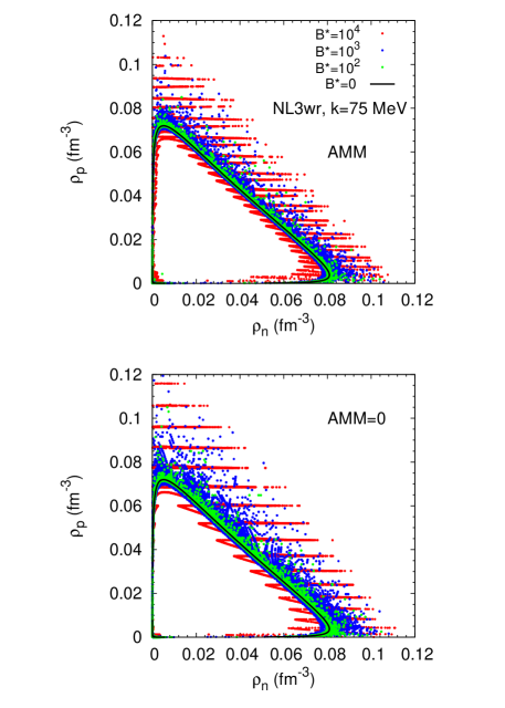
Figure 1: Dynamical spinodal for NL3$\omega\rho$, a momentum transfer of $k=75$ MeV, and $B^{*}=10^{4}$ (red), $B^{*}=10^{3}$ (blue), and $B^{*}=10^{2}$ (green) with AMM (top) and without AMM (bottom). A comparison with the $B=0$ (black lines) results is also made.

In the present section, we discuss the effects of strong magnetic fields on the structure of the inner crust of magnetars. In particular, we analyse the dynamical spinodals for the NL3$\omega\rho$ model for three different values of the magnetic field: $B=4.41\times 10^{15}$ G, $B=4.41\times 10^{16}$ G, and $B=4.41\times 10^{17}$ G. These values correspond to $B^{*}=10^{2}$, $B^{*}=10^{3}$, and $B^{*}=10^{4}$, where $B=B^{*}B_{ce}$, with $B_{ce}=4.41\times 10^{13}$ G, being the electron critical magnetic field. In fact, the most intense fields detected on the surface of a magnetar are not larger than $2\times 10^{15}$ G, i.e. one or two orders of magnitude smaller than the two more intense fields considered in this study. However, in Refs. kiuchi08 ; rezzolla12 , the authors obtained toroidal fields more intense than 10¹⁷G in stable configurations, meaning that in the interior of the stars, stronger fields may be expected.

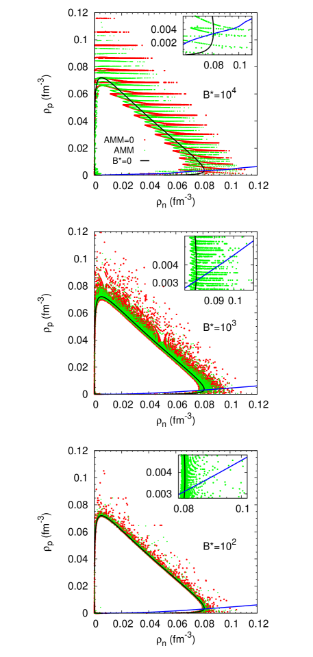
Figure 2: Dynamical spinodal for NL3$\omega\rho$, a momentum transfer of $k=75$ MeV, with AMM (green) and without AMM (red), for $B^{*}=10^{4}$ (top), $B^{*}=10^{3}$ (middle), and $B^{*}=10^{2}$ (bottom). A comparison with the $B=0$ (black lines) results is also made. The EoS for $\beta-$equilibrium matter is also shown.

In Fig. 1, we show the dynamical spinodal sections in the ($\rho_{p}$,$\rho_{n}$) space for the magnetic fields mentioned above, with (top) and without (bottom panels) AMM. The black lines represent the spinodal section when the magnetic field is zero. The calculations were performed with $k=75$ MeV, which is a value of the transferred momentum that gives a spinodal section very close to the envelope of the spinodal sections. These sections have been obtained numerically by solving the dispersion relation (36) for $\omega=0$. This was performed looking for the solutions at a fixed proton fraction, and for each solution, a point was obtained. The solutions form a large connected region for the lower proton and neutron densities, plus extra disconnected domains that do not occur at $B=0$. The point-like appearance of the sections is a numerical limitation. A higher resolution in ($\rho_{p}$,$\rho_{n}$) would complete the gaps.

First we compare the results obtained omitting the AMM contribution (bottom panel). The structure of the spinodal section obtained for the strongest field considered, $B^{*}=10^{4}$, clearly shows the effect of the Landau quantization, as already shown in Ref. fang16 : there are instability regions that extend to much larger densities than the $B=0$ spinodal section, while there are also stable regions that at $B=0$ would be unstable. This is due to the fact that the energy density becomes softer, just after the opening of a new Landau level, and harder when the Landau level is most filled. The spinodal section has a large connected section at the lower densities and extra disconnected regions. If smaller fields are considered, the structure found for $B^{*}=10^{4}$ is still present, but at a much smaller scale due to the increase of the number of Landau levels, see detail in the inset of the middle panel of Fig. 2, for $B^{*}=10^{3}$. It is clear that the spinodal section tends to the $B=0$ one, as the magnetic field intensity is reduced.

In the top panel of Fig. 1, we show the same three spinodal sections, but with the inclusion of the AMM for the protons and neutrons. The overall conclusions taken for the spinodals without the AMM are still valid, although the section acquires more structure when the AMM is included since, for each Landau level, the proton spin up and spin down levels have different energies. This difference originates a doubling of the bands, which are easily identified for $B^{*}=10^{4}$. Besides, these bands are also affected by the neutron AMM. The spinodal sections obtained with AMM are smaller, as it is seen from Fig. 2, where, for each field intensity, $B^{*}=10^{4}$ (top), $10^{3}$ (middle), and $10^{2}$ (bottom), the spinodal section without (red) and with (green) AMM are plotted. Although the inclusion of the AMM does not have a very strong effect because the proton and neutron anomalous magnetic moments are small, these effects are not negligible, and, in fact, they reduce the instability sections. In the three panels of Fig. 2, we include an inset panel where we have zoomed in the spinodal with AMM in a small range of densities to show that, although in a smaller scale, the structure is similar to the one shown for $B^{*}=10^{4}$.

For neutron-rich matter, as the one occurring in neutron stars, the instability regions extend to densities almost 40% larger than the crust-core transition density for $B=0$. The effect of the magnetic field is larger precisely when the proton fraction is smaller. We have included in the three panels of Fig. 2 a curve that represents the densities ($\rho_{p},\rho_{n}$) at $\beta$-equilibrium, including the contribution of the AMM. The curves cross an alternation of stable and unstable regions, indicating the existence of a complex crust-core transition, see the insets for detail. The beginning of an homogeneous matter is shifted to larger densities, 0.100 fm^-3 for $B^{*}=10^{4}$, 0.103 fm^-3 for $B^{*}=10^{3}$, and 0.105 fm^-3 for $B^{*}=10^{2}$, corresponding to the pressures 0.818 MeV$/$ fm³, 0.833 MeV$/$ fm³, and 0.863 MeV$/$ fm³, respectively. This complex transition region with a thickness of $\sim 0.02$ fm^-3, even for the weaker fields, will have strong implications in the structure of the inner crust of magnetars.

We will discuss later in more detail the crust-core transition region in the presence of magnetic fields.

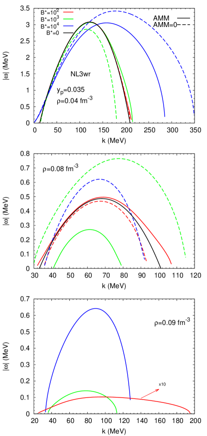
Figure 3: Growth rates, $|\omega|$, as a function of the momentum, $k$, for NL3$\omega\rho$, a proton fraction of $y_{p}=0.035$, and $B^{*}=10^{2}$ (red), $B^{*}=10^{3}$ (black), and $B^{*}=10^{4}$ (blue) with AMM (solid) and without AMM (dashed lines), for a fixed baryonic density of $\rho=0.04$ fm^-3 (top), $\rho=0.08$ fm^-3 (middle), and $\rho=0.09$ fm^-3 (bottom). The growth rates for $B^{*}=10^{2}$ in the bottom panel are multiplied by a factor of 10 and are obtained for $\rho=0.0903$ fm^-3.

The solution of the dispersion relation inside the spinodal section gives pure imaginary frequencies, indicating that the system is unstable to the propagation of a perturbation with the corresponding wave number in the density range where this occurs. The modulus of the frequency, designated as growth rate, indicates how the system evolves into a two-phase configuration. The evolution will be dictated by the largest growth rate chomaz04 ; providencia06 .

As an example, in Fig. 3, we show the growth rates, $|\omega|$, as a function of the transferred momentum $k$, for fixed values of the baryonic density: $\rho=0.04$ fm³ (top), $\rho=0.08$ fm³ (middle), and $\rho=0.09$ fm³ (bottom panels). We consider a fixed proton fraction of 0.035, which is an average value found for NL3$\omega\rho$ within a Thomas-Fermi calculation of the inner crust grill12 , and we choose the same values for the magnetic field as in the previous figures. The growth rates with (solid) and without (dashed) AMM are plotted together with the growth rate at $B=0$ (black line).

We first consider $\rho=0.04$ fm^-3, far from the transition to homogeneous matter. The smaller the field, the smaller the effect of the AMM, and for $B^{*}=10^{2}$, the two curves superimpose, and are almost coincident with the $B=0$ result. The effect of the AMM for the two larger fields is non-negligible, and may go in opposite direction because its behavior is closely related with the filling of the Landau levels. The instability does not exist for the two smaller fields at $k$ close to zero. This is the behavior discussed in Ref. providencia06 and is directly related to the $1/k^{2}$ divergence of the Coulomb field. However, for $B^{*}=10^{4}$, and since the electron and proton densities are small, the attractive nuclear interaction is strong enough to drag the electrons, keeping the instability until $k=0$. This is not anymore the case for the two larger densities considered, because in these two cases, the nuclear interaction is not able to compensate for the larger densities of charged particles. The stronger nuclear attraction for $B^{*}=10^{4}$ is also observed for the large values of $k$: the instability is still present for $k>300$ MeV, well above the maximum $k$ attained for $B=0$, indicating that the attractiveness of the nuclear force is stronger at short ranges.

The two larger densities have been chosen because they are at the $B=0$ crust-core transition or above, and this is the most sensitive region to the presence of a strong magnetic field. Due to the alternation between stable and unstable regions, it is highly probable that for one of the field intensities, no instability is present for the particular density value considered. This explains the non appearance of the curve with AMM for $B^{*}=10^{4}$ and $\rho=0.08$ fm^-3. It also explains why the behaviors with and without AMM are so different for $B^{*}=10^{3}$: the value of the density considered picks up the instability region more or less close to the limit of the instability region. In this case, also the maximum growth rates occur for different wave numbers. For $B^{*}=10^{2}$, the results with and without AMM differ, and are not anymore coincident with the $B=0$ result, as seen for $\rho=0.04$ fm^-3. However, the maximum growth rate occurs at similar wave numbers in the three cases.

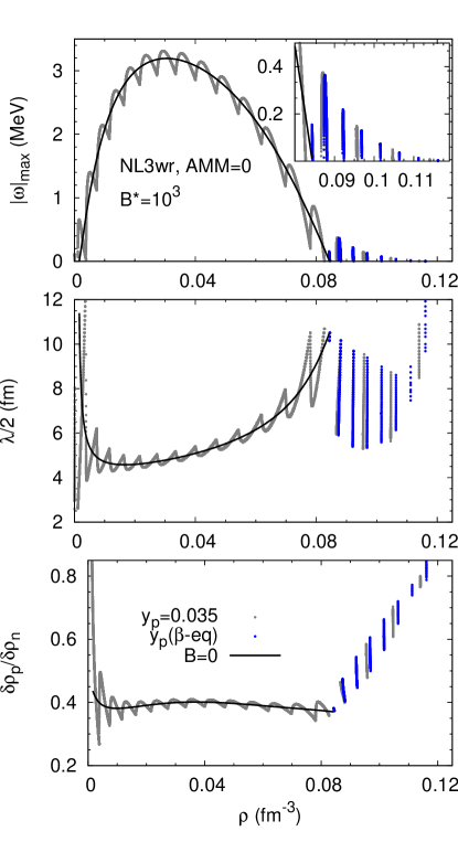
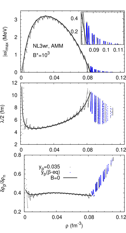
Figure 4: Largest growth rate (top panels), the corresponding half-wavelength (middle panels), and the proton-neutron density fluctuation ratio (bottom panels) versus density for NL3$\omega\rho$, and a magnetic field of $B^{*}=10^{3}$, without (left panels) and with (right panels) AMM. Results with the $B=0$ (black solid lines) calculation are also shown for comparison. The blue points correspond to a calculation with a proton fraction equal to the one found in $\beta-$equilibrium matter, above $\rho_{t}=0.0843$ fm^-3, the $B=0$ crust-core transition density. The gray points correspond to a fixed proton fraction of 0.035 in the whole density range.

Finally, we consider the larger density, $\rho\sim 0.09$ fm^-3, approximately 10% above the crust-core transition density, when no field is considered. For $B=0$, this density belongs to the core, and corresponds to homogeneous matter. However, for the three intensities of the magnetic field we have been considering, $B^{*}=10^{2},\,10^{3},\,10^{4}$, this is inside or close to a region of instability. For $B^{*}=10^{2}$, we have taken $\rho=0.0903$ fm^-3, and multiplied the growth rate by a factor of 10 in the figure. We conclude that the growth rates decrease with the magnetic field, showing a convergence for the $B=0$ result when no instability exists.

In the following, we shall consider that the behavior of the system will be determined by the largest growth rate, $|\omega|_{max}$, the mode that drives the system into a separation of a high and a low density phases. As in Ref. providencia06 , we will consider that half wave-length of the maximum growth rate mode is a good estimation of the order of magnitude of the size of the clusters which are formed, as shown in Ref. avancini08 , where the size of the clusters obtained within a Thomas-Fermi calculation were compared with the half-wave length associated to the most unstable mode. These quantities are plotted in Figs. 4, and 5.

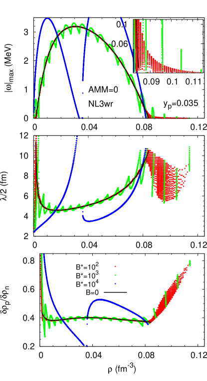
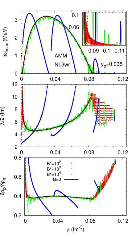
Figure 5: Largest growth rate (top panels), the corresponding half-wavelength (middle panels), and the proton-neutron density fluctuation ration (bottom panels) versus density for NL3$\omega\rho$, with a proton fraction of $y_{p}=0.035$, and without (left panels) and with (right panels) AMM. Three different values of $B$ are considered: $B^{*}=10^{2}$ (red), $B^{*}=10^{3}$ (green), and $B^{*}=10^{4}$ (blue). A comparison with the $B=0$ (black lines) results is also made.

In Fig. 4, the largest growth rates (top panels), the corresponding half-wave length (middle panels), and the $\delta\rho_{p}/\delta\rho_{n}$ ratio are shown for $B^{*}=10^{3}$. The left panels show the calculations performed without AMM, and the right panels take the AMM into account. In all figures, the $B=0$ results are represented by a black curve, in grey we show the results with a fixed proton fraction of 0.035, and in blue we take, above the $B=0$ crust-core transition density, the proton fraction as the one found in $\beta-$equilibrium matter. In Fig. 5, the same quantities calculated with three different magnetic field intensities, $B^{*}=10^{2},10^{3}$, and $10^{4}$, are compared. In this figure, all results were obtained with a fixed proton fraction $y_{p}=0.035$.

Table 1: Transition densities and pressures for the magnetic fields considered in this study, together with the correspondent fractional moment of inertia of the neutron star crust, for a star of $M=1.4$ M_⊙ and $R=13.734$ km. Also shown are the crust thicknesses, $\Delta R$, the thickness due to the inhomogeneous region found when $B\neq$0, $\Delta R^{\prime}=R(\rho_{1})-R(\rho_{2})$, and the difference to the $B=0$ result, $\Delta R_{B}=\Delta R-\Delta R(B=0)$. The results shown take into account AMM. The transition densities are calculated when $|\omega|=0$ (see top panels of Figs. 4 and 5, and the text for more details). The values for $\rho_{2}$ correspond to the calculations with a $\beta-$equilibrium matter proton fraction.

$B^{*}$	$\rho_{1}$	$\rho_{2}$	$P_{1}$	$P_{2}$	$\Delta R$	$\Delta R^{\prime}$	$\Delta R_{B}$	$\frac{\Delta I_{cr}}{I}$
	(fm-3)	(fm-3)	$\left(\frac{\mbox{MeV}}{\mbox{fm}^{3}}\right)$	$\left(\frac{\mbox{MeV}}{\mbox{fm}^{3}}\right)$	(m)	(m)	(m)
0	0.0843	0.0843	0.5196	0.5196	1368	0	0	0.0676
$10^{2}$	0.0837	0.1044	0.5119	0.8541	1551	185	182	0.0968
$10^{3}$	0.0808	0.1096	0.4758	0.9743	1609	257	240	0.1056
$10^{4}$	0.0654	0.0998	0.3274	0.8095	1503	260	134	0.0922

The effect that had already been identified with the spinodal sections is clearly shown in theses figures: the unstable regions occur well beyond the $B=0$ crust-core transition at 0.0843 fm^-3, and extend until $\rho_{t}=0.11$ fm^-3, 40% larger than the $B=0$ transition density. However, above 0.082 fm^-3, the unstable regions alternate with stable ones. This effect was first discussed in Ref. fang16 . The transition densities that define the limits of the region of alternating stable and unstable regions have been labelled $\rho_{1}$ and $\rho_{2}$, and are shown in Table 1. The transition density $\rho_{1}$ defines the first time $|\omega|$ goes to zero, and the density $\rho_{2}$ defines the onset of the homogeneous matter, meaning that we have a range of densities between $\rho_{1}$ and $\rho_{2}$ where unstable and stable regions alternate. At $B=0$, both densities coincide, i.e. $\rho_{1}=\rho_{2}$. The density $\rho_{2}$ is determined by taking the $\beta-$equilibrium matter proton fraction above the $B=0$ crust-core transition, and $\rho_{1}$ is calculated with the fixed $y_{p}=0.035$ proton fraction, obtained from the $B=0$ calculations of the pasta phases, since $\rho_{1}$ is a density that lies below the $B=0$ crust-core transition. Taking the $\beta$-equilibrium proton fraction, instead of the fixed 0.035, has a non-negligible effect, and, in fact, reduces the instability region, because the $\beta$-equilibrium condition predicts larger proton fractions, and the larger the proton densities, the smaller the effects due to the magnetic field. In particular, for $B^{*}=10^{4}$, $\rho_{2}$ is $\sim 0.01$ fm^-3 smaller, taking $y_{p}^{\beta-eq}$ instead of $y_{p}=0.035$. This difference is $\sim 0.005$ fm^-3 for $B^{*}=10^{2}$, and $\sim 0.002$ fm^-3 for $B^{*}=10^{3}$. The discrete feature of the Landau levels results in a non-monotonic behavior of this quantity for the larger values of $B^{*}$.

Besides $\rho_{1}$ and $\rho_{2}$, in Table 1, we also give the pressure at these two densities and the fractional moment of inertia of the crust, a quantity that depends directly on the pressure and density at the crust-core transition, and that has an important impact in explaining pulsar glitches. The fractional moments of inertia were calculated from the approximate expression given in Worley08 ; Lattimer00 :

$$\frac{\Delta I_{cr}}{I} \simeq \frac{28\pi P_{t}R^{3}}{3M}\frac{(1-1.67\beta-0.6\beta^{2})}{\beta}$$ (39)

$$\times \left[1+\frac{2P_{t}(1+5\beta-14\beta^{2})}{\rho_{t}m_{b}\beta^{2}}\right]^{-1}\,,$$

where $\Delta I_{cr}$ is the crust moment of inertia, $I$ is the total star moment of inertia, $P_{t}$ and $\rho_{t}$ are the crust-core transition pressure and density, respectively, $M$ and $R$ are the gravitational mass and radius of the star, $\beta=GM/R$ is the compactness parameter, and $m_{b}$ is the nucleon mass. In Table 1, the crust thickness, $\Delta R=R(0)-R(\rho_{2})$, the thickness of the region between $\rho_{1}$ and $\rho_{2}$, $\Delta R^{\prime}=R(\rho_{1})-R(\rho_{2})$, and the difference between the crust thicknesses at $B=0$ and $B\neq 0$, $\Delta R_{B}=\Delta R-\Delta R(B=0)$, are also displayed. These results take into account the AMM, and they have been calculated for a star with $M=1.4$ M_⊙, and a radius of $R=13.734$ km. For the calculation of the fractional moment of inertia of the crust, we took for $P_{t}$ and $\rho_{t}$ the values of $P_{2}$ and $\rho_{2}$, given in the Table for each magnetic field. Our results for $B=0$ agree with the transition densities and pressures and the moment of inertia of the crust obtained in Ref. fattoyev10 , see tables III and IV. This is expectable, since the same expression for the crustal moment of inertia has been used, as in Refs. Worley08 ; Lattimer00 .

The magnetic field gives rise to larger values of the crust-core transition pressure and density, and these affect directly $\Delta I_{crust}/{I}$. These values are much higher than the prediction in link99 ; glitch2 for the Vela pulsar, 0.016, when no entrainment effects are considered, and they would be high enough for the crust to completely describe the glitch mechanism, even taking into account the effect of entrainment glitch2 ; chamel13 . In fact, in this case the “effective” moment of inertia associated with the fluid is lowered and the constraint inferred from glitches requires that the crustal moment of inertia is $\langle m^{*}_{n}\rangle/m_{n}\sim 4-6$ larger glitch2 , where $m^{*}_{n}$ is the effective neutron mass including entrainment, and $m_{n}$ the bare neutron mass. To explain the Vela glitches, this constraint would be equivalent to requiring a fractional crustal moment of inertia $\sim 0.064-0.096$.

The calculation including the AMM of protons and neutrons presents twice as much unstable regions due to the separation of each proton Landau level in two, with a different spin polarization. The resulting regions are narrower and have smaller growth rates. More information on the properties of this range of densities is obtained from the middle and bottom panels of both Figures. In the middle panel, the half-wave length of the perturbation is plotted, and it gives an estimation of the size of the cluster that will be formed. Within each of these independent unstable regions, the cluster size changes from about 9 fm to about 4 fm in a very narrow density range. Finally, the bottom panel gives some information on the proton content of the dense phase: the clusters will be quite proton rich with a proton-neutron density fluctuation ratio well above the 0.04 ratio of the homogeneous matter.

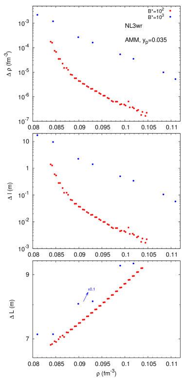
Figure 6: Width of the instability peaks, $\Delta\rho$, (top panel), the thickness of the instability regions, $\Delta l$ (middle panel), and the distance between the instabilities, $\Delta L$ (bottom panel), as a function of the baryonic density, for NL3$\omega\rho$, a proton fraction of $y_{p}=0.035$, $B^{*}=10^{2}$ (red), and $B^{*}=10^{3}$ (blue), with AMM. In the bottom panel, $\Delta L$ obtained with $B^{*}=10^{3}$ is multiplied by a factor of 0.1.

For $B^{*}=10^{2}$ and $10^{3}$, we have made an analysis of the dependence on the density of the width and separation of the instability peaks above the transition density, $\rho_{t}(B=0)$. In the top panel of Fig. 6, the width of these peaks, $\Delta\rho$, is plotted versus the density, and it is seen that it decreases exponentially, showing a steeper decrease for $B^{*}=10^{2}$. We may ask what is the impact of these structures in the neutron star, and, in particular, what is their size. In order to make an estimation, we have considered a 1.4 $M_{\odot}$ star profile, and calculated the localization of the instabilities. This has allowed the determination of the thickness of the instability regions, $\Delta l$, in meters, and the distance between the instabilities, $\Delta L$, also in meters. The results are shown in the middle and bottom panels of Fig. 6, respectively. Some conclusions are in order: for $B^{*}=10^{2}$, the spacing between peaks increases with density from $\sim 6$ m to $~{}\sim 9$ m, until the homogeneous core sets in, while for $B^{*}=10^{3}$, this spacing is one order of magnitude larger; the width of the peaks decreases exponentially from $\sim 1$ m for $\rho=0.085$fm^-3 to $\sim 5$ mm for $\rho=0.1$fm^-3 for $B^{*}=10^{2}$, and is 1-2 orders of magnitude larger if $B^{*}=10^{3}$. In the bottom panel, we may identify two almost parallel curves which correspond to the distance between peaks with the polarization aligned or anti-aligned with the magnetic field.

These properties indicate that at the crust-core transition, matter is very complex and that the magnetic field favors the large charge concentration in the clusters. Even considering matter below the $B=0$ crust-core transition, the present calculation indicates that there is a fast change of the cluster size. This change will probably cause the cluster size and structure to change more strongly with density than it would be expected for $B=0$, giving rise to more heterogeneous matter.

Simulations of the time evolution of the magnetic field at the crust have shown that the existence of amorphous and heterogeneous matter deep in the inner crust, with a high impurity parameter and, therefore, highly resistive, favors a fast decay of the magnetic fields. This has been proposed as an explanation for the non-observation of x-ray pulsars with a period above 12 s pons13 .

IV Conclusions

We present a formalism to calculate the eigenmodes of nuclear and stellar matter in the presence of very strong magnetic fields, as may be found in magnetars. The AMM of protons and neutrons is taken into account and it is shown that it is not negligible for magnetic fields above 10¹⁵ G. Within this formalism, it is possible to estimate the crust-core transition inside neutron stars from the spinodal section, the surface where the eigenmodes go to zero. Inside these surfaces, matter will separate into a dense and a gas phase. This RMF description of stellar matter takes into account both the Coulomb field and finite size effects related to the finite range of nuclear force. We have only considered the propagation of waves in the direction of the magnetic field.

The main objective of this work was to complete the discussion published in Ref. fang16 , where the linearized Vlasov equation was used to determine the importance of taking into account explicitly the effect of magnetic fields of the order of 10¹⁵-$10^{17}$ G on the description of stellar matter at subsaturation densities, in particular, the effect of the magnetic field on the crust-core transition in magnetized neutron stars. It was shown in Refs. broderick ; broderick02 that only fields two to three orders of magnitude stronger than the critical electron magnetic field have a finite effect on the EoS at densities above saturation density, but no discussion has been presented for lower densities of interest for the inner crust. However, in Refs. chamel12 ; chamel15 , the non-negligible effect of the magnetic field on the properties of the outer crust has already been discussed. Even though the largest fields detected on the surface of magnetars are 2$\times 10^{15}$ G on the SGR 1806−20 (see e.g. olausen14 and the McGill Online Magnetar Catalog sgr ), we expect that stronger fields are still realistic, because in Refs. kiuchi08 ; rezzolla12 equilibrium configurations of magnetars with fields well above 10¹⁵ G in the interior have been obtained when a toroidal component of the magnetic field is considered.

The effect of the Landau quantization of the levels of charged particles gives rise to a spinodal section that presents a structure of bands at the border between clusterized and homogeneous matter. As a consequence, it was shown that the transition between the crust and the core of magnetars is defined by a complex region that is $\sim 0.02-0.04$ fm^-3 wide, characterized by a succession of homogeneous and clusterized matter. Calculations have been performed with and without the inclusion of the AMM, and it was shown that the AMM has a non-negligible effect, and, moreover, it contributes to an extra complexity of matter at the crust-core transition.

The determination of the mode associated with the maximum growth rate in the density range delimited by the spinodal section, allowed the estimation of several properties of the clusters that are formed in the unstable regions, in particular, the size and a qualitative charge content. Two different density regions should be considered independently: a) inside the density region delimited by the $B=0$ spinodal, the size and the $\delta\rho_{p}/\delta\rho_{n}$ ratio change along the trend defined by the corresponding $B=0$ results, showing fluctuations around these values, the larger the field the larger the fluctuations; b) the density region outside the $B=0$ spinodal section, where an alternation of unstable and stable regions occurs. In this region, the clusters formed inside the unstable regions vary between $\sim 5-10$ fm inside very small density ranges, and the larger the densities, the larger the proton fraction inside the clusters. In a 1.4 $M_{\odot}$ star, this region has a width of $\sim 200$ m for $B^{*}=10^{2}$, and a bit larger for $B^{*}=10^{3}$ and $10^{4}$. If $B^{*}=10^{2}$, the spacing between peaks is $\sim 6-9$ m, and the width of the peaks decreases exponentially from 1 m at the $B=0$ crust-core transition, to $2\times 10^{-3}$ m at the onset of homogeneous matter. For $B^{*}=10^{3}$ these quantities are 1-2 orders of magnitude larger. Including this complex region in the crust, the crust moment of inertia can be as large as 9-10% the total star moment of inertia, circa 30% larger than the ratio obtained for $B=0$.

These results indicate that it is necessary to study the transport properties, such as electric conductivity and shear viscosity, of this complex matter, see yakovlev15 ; yakovlev15a . Also, the overall properties obtained for stellar matter at subsaturation densities seem to support the occurrence of a larger electrical resistivity in the presence of a strong magnetic field, supporting the existence of a resistive layer deep inside the inner crust of magnetized neutron stars, as proposed in Ref. pons13 , that would cause a fast decay of the magnetic field, and explain the non-observation of isolated pulsars, with periods larger than 12 s.

Appendix

The coefficients $a_{ij}$ of the matrix (36) can be written as:

$$a_{11} = \sum_{\nu,s}\frac{g_{s}}{2\pi^{2}}\frac{G_{\phi_{p}}M^{*}}{\omega_{s}^{2}}\frac{eB}{P_{F}^{p}(s_{p}^{2}-1)},$$

$$a_{12} = -\sum_{\nu,s}\frac{eB}{2\pi^{2}V_{F}^{p}(s_{p}^{2}-1)}\left[\left(1-\frac{\omega^{2}}{k_{z}^{2}}C_{1p}\right)g_{v}D_{1p}\right.$$

$$+ \left.\left(1-\frac{\omega^{2}}{k_{z}^{2}}C_{2p}\right)\frac{g_{\rho}}{2}D_{2p}+\left(1-\frac{\omega^{2}}{k_{z}^{2}}\right)\frac{e^{2}}{\omega_{A}^{2}}\right]-1,$$

$$a_{13} = \sum_{\nu,s}\frac{g_{s}}{2\pi^{2}}\frac{G_{\phi_{p}}M^{*}}{\omega_{s}^{2}}\frac{1}{V_{F}^{p}\epsilon_{F}^{n}(s_{p}^{2}-1)},$$

$$a_{14} = -\sum_{\nu,s}\frac{1}{2\pi^{2}V_{F}^{p}(s_{p}^{2}-1)}\left[\left(1-\frac{\omega^{2}}{k_{z}^{2}}C_{1p}\right)g_{v}D_{1n}\right.$$

$$+ \left.\left(1-\frac{\omega^{2}}{k_{z}^{2}}C_{2p}\right)\frac{g_{\rho}}{2}D_{2n}\right],$$

$$a_{15} = \sum_{\nu,s}\left(1-\frac{\omega^{2}}{k_{z}^{2}}\right)\frac{e^{2}}{2\pi^{2}\omega_{A}^{2}}\frac{eB}{V_{F}^{p}(s_{p}^{2}-1)},$$

$$a_{21} = \frac{\bar{m}_{p}}{\tilde{m}_{p}}a_{11}-1,\quad a_{22}=\frac{\bar{m}_{p}}{\tilde{m}_{p}}(a_{12}+1),$$

$$a_{23} = \frac{\bar{m}_{p}}{\tilde{m}_{p}}a_{13},\quad a_{24}=\frac{\bar{m}_{p}}{\tilde{m}_{p}}a_{14},\quad a_{25}=\frac{\bar{m}_{p}}{\tilde{m}_{p}}a_{15},$$

$$a_{31} = \sum_{s}\frac{g_{s}M^{*}}{(2\pi)^{2}}\frac{eB}{\omega_{s}^{2}\epsilon_{F}^{p}}\epsilon_{F}^{n}P_{F}^{n}L^{*}(s_{n}),$$

$$a_{32} = -\sum_{s}\left[\left(1-\frac{\omega^{2}}{k_{z}^{2}}C_{1n}\right)g_{v}D_{1p}-\left(1-\frac{\omega^{2}}{k_{z}^{2}}C_{2n}\right)\frac{g_{\rho}}{2}D_{2p}\right]$$

$$\times\frac{eB}{4\pi^{2}}\epsilon_{F}^{n}P_{F}^{n}L(s_{n}),$$

$$a_{33} = \sum_{s}\frac{g_{s}M^{*}}{(2\pi)^{2}}\frac{P_{F}^{n}}{\omega_{s}^{2}}L^{*}(s_{n}),$$

$$a_{34} = -\sum_{s}\left[\left(1-\frac{\omega^{2}}{k_{z}^{2}}C_{1n}\right)g_{v}D_{1n}-\left(1-\frac{\omega^{2}}{k_{z}^{2}}C_{2n}\right)\frac{g_{\rho}}{2}D_{2n}\right]$$

$$\times\frac{\epsilon_{F}^{n}P_{F}^{n}L(s_{n})}{4\pi^{2}}-1,$$

$$a_{35} = 0,$$

$$a_{41} = a_{31}\frac{H^{*}(s_{n})}{L^{*}(s_{n})},\quad a_{42}=a_{32}\frac{H(s_{n})}{L(s_{n})},$$

$$a_{43} = a_{33}\frac{H^{*}(s_{n})}{L^{*}(s_{n})}-1,$$

$$a_{44} = (a_{34}+1)\frac{H(s_{n})}{L(s_{n})},\quad a_{45}=0,$$

$$a_{51} = a_{53}=a_{54}=0,$$

$$a_{52} = \sum_{\nu,s}\left(1-\frac{\omega^{2}}{k_{z}^{2}}\right)\frac{e^{2}}{2\pi^{2}\omega_{A}^{2}}\frac{eB}{V_{F}^{e}(s_{e}^{2}-1)},$$

$$a_{55} = -\sum_{\nu,s}\left(1-\frac{\omega^{2}}{k_{z}^{2}}\right)\frac{e^{2}}{2\pi^{2}\omega_{A}^{2}}\frac{eB}{V_{F}^{e}(s_{e}^{2}-1)}-1$$

where $\tilde{m}_{p}=\bar{m}_{p}+s\mu_{N}\kappa_{p}B$, $\omega_{s}^{2}=\omega^{2}-k_{z}^{2}-m^{2}_{s,eff}$, $\omega_{A}^{2}=\omega^{2}-k_{z}^{2}$, and $s_{i}=\frac{\omega}{\omega_{0i}},\,i=p,n,e.$

The remaining coefficients are given by

$$G_{\phi_{p}} = \frac{g_{s}M^{*}\bar{m}_{p}}{\epsilon_{F}^{p}(\bar{m}_{p}+s\mu_{N}\kappa_{p}B)},$$

$$G_{\phi_{n}} = \frac{g_{s}M^{*}}{\epsilon_{F}^{n}}\left(1-\frac{s\mu_{N}\kappa_{n}B}{\sqrt{M^{*2}+P_{F}^{n2}(1-x^{2})}}\right),$$

$$C_{1i} = 1-\frac{\tau_{i}g_{\rho}\chi}{2g_{v}\omega_{\rho}^{2}},$$

$$C_{2i} = 1-\frac{2\tau_{i}g_{v}\chi}{g_{\rho}\omega_{v}^{2}},$$

$$D_{1i} = \frac{\tau_{i}g_{\rho}\chi}{2D_{\nu}}+\frac{g_{v}\omega_{\rho}^{2}}{D_{\nu}},$$

$$D_{2i} = \frac{g_{v}\chi}{D_{\nu}}+\frac{\tau_{i}g_{\rho}\omega_{v}^{2}}{2D_{\nu}},$$

$$D_{\nu} = \omega_{v}^{2}\omega_{\rho}^{2}-\chi,$$

$$L(s_{n}) = \int_{-1}^{1}\frac{x}{(s_{n}-x)}dx,\quad L^{*}(s_{n})=\int_{-1}^{1}\frac{G_{\phi_{n}}xdx}{(s_{n}-x)},$$

$$H(s_{n}) = \int_{-1}^{1}\left(1-\frac{s\mu_{N}\kappa_{n}B}{\sqrt{M^{*2}_{n}+P_{F}^{n2}(1-x^{2})}}\right)\frac{xdx}{(s_{n}-x)},$$

$$H^{*}(s_{n}) = \int_{-1}^{1}\left(1-\frac{s\mu_{N}\kappa_{n}B}{\sqrt{M^{*2}_{n}+P_{F}^{n2}(1-x^{2})}}\right)\frac{G_{\phi_{n}}xdx}{(s_{n}-x)}.$$

The amplitudes of the scalar densities fluctuations, $A^{is}_{\omega,\nu,s}$, and of the vector densities fluctuations, $A^{i}_{\omega,\nu,s}$, are given by

$$A_{\omega,\nu,s}^{ps} = \sum_{\xi}\xi\frac{\bar{m}_{p}}{(\bar{m}_{p}+s\mu_{N}\kappa_{p}B)}S_{\omega,\nu,s}^{p}(\xi),$$

$$A_{\omega,s}^{ns} = \int_{-1}^{1}P_{F}^{n2}x\left(1-\frac{s\mu_{N}\kappa_{n}B}{\sqrt{M^{*2}_{n}+P_{F}^{n2}(1-x^{2})}}\right)S_{\omega,s}^{n}dx,$$

$$A_{\omega,\nu,s}^{p} = \sum_{\xi}\xi S_{\omega,\nu,s}^{p}(\xi),$$

$$A_{\omega,s}^{n} = \int_{-1}^{1}P_{F}^{n2}xS_{\omega,s}^{n}dx,$$

$$A_{\omega,\nu,s}^{e} = \sum_{\xi}\xi S_{\omega,\nu,s}^{e}(\xi),$$

References

• (1) R. C. Duncan and C. Thompson, Astrophys. J. 392, L9 (1992); C. Thompson and R. C. Duncan, Mon. Not. R. Astron. Soc. 275, 255 (1995).
• (2) V. V. Usov, Nature 357, 472 (1992).
• (3) B. Paczyński, Acta Astron. 42, 145 (1992).
• (4) SGR/APX online Catalogue, http://www.physics.mcgill.ca/~pulsar/magnetar/main.html
• (5) J. A. Pons, D. Viganò, and N. Rea, Nature Phys. 9,431 (2013).
• (6) D. G. Ravenhall, C. J. Pethick, and J. R. Wilson, Phys. Rev. Lett. 50, 2066 (1983).
• (7) C. J. Horowitz, M. A. Pérez-García, and J. Piekarewicz, Phys. Rev. C 69, 045804 (2004); Hidetaka Sonoda, Gentaro Watanabe, Katsuhiko Sato, Kenji Yasuoka, and Toshikazu Ebisuzaki, Phys. Rev. C 77, 035806 (2008); A. S. Schneider, D. K. Berry, C. M. Briggs, M. E. Caplan, and C. J. Horowitz, Phys. Rev. C 90, 055805 (2014).
• (8) H. Shen, H. Toki, K. Oyamatsu, K. Sumiyoshi, Nucl. Phys. A 637, 435 (1998).
• (9) T. Maruyama, T. Tatsumi, D. Voskresensky, T. Tanigawa, and S. Chiba, Phys. Rev. C 72, 015802 (2005).
• (10) S. S. Avancini, D. P. Menezes, M. D. Alloy, J. R. Marinelli, M. M. W. Moraes, and C. Providência, Phys. Rev. C 78, 015802 (2008).
• (11) W. G. Newton and J. R. Stone, Phys. Rev. C 79, 055801 (2009).
• (12) H. Pais and J. R. Stone, Phys. Rev. Lett. 109, 151101 (2012).
• (13) P. Gögelein, and H. Müther, Phys. Rev. C 76, 024312 (2007).
• (14) M. Oertel, M. Hempel, T. Klähn, and S. Typel, arXiv:1610.03361 [astro-ph.HE].
• (15) C. J. Horowitz, D. K. Berry, C. M. Briggs, M. E. Caplan, A. Cumming, and A. S. Schneider, Phys. Rev. Lett. 114, 031102 (2015); A. S. Schneider, D. K. Berry, M. E. Caplan, C. J. Horowitz, and Z. Lin, Phys. Rev. C 93, 065806 (2016).
• (16) D. G. Yakovlev, Mon. Not. R. Astron. Soc. 453, 581 (2015).
• (17) H. Mueller, and B. D. Serot, Phys. Rev. C 52, 2072 (1995).
• (18) M. Colonna, Ph. Chomaz, and S. Ayik, Phys. Rev. Lett. 88, 122701 (2002).
• (19) Ph. Chomaz, M. Colonna, and J. Randrup, Phys. Rep. 389, 263 (2004).
• (20) C. Providência, L. Brito, S. S. Avancini, D. P. Menezes, and Ph. Chomaz, Phys. Rev. C 73, 025805 (2006).
• (21) S. S. Avancini, S. Chiacchiera, D. P. Menezes, and C. Providência, Phys. Rev. C 82, 055807 (2010).
• (22) Aaron Worley, Plamen G. Krastev, and Bao-An Li, Astrophys. J. 685, 390 (2008).
• (23) J. M. Lattimer and M. Prakash, Phys. Rep. 333, 121 (2000).
• (24) B. Link, R. I. Epstein, and J. M. Lattimer, Phys. Rev. Lett. 83, 3362 (1999).
• (25) N. Andersson, K. Glampedakis, W. C. G. Ho, and C. M. Espinoza, Phys. Rev. Lett. 109, 241103 (2012).
• (26) N. Chamel, Phys. Rev. C 85, 035801 (2012); Phys. Rev. Lett 110, 011101 (2013).
• (27) M. Nielsen, C. Providência, and J. da Providência, Phys. Rev. C 44, 209 (1991).
• (28) L. Brito, C. Providência, A. M. Santos, S. S. Avancini, D. P. Menezes, and Ph. Chomaz, Phys. Rev. C 74, 045801 (2006).
• (29) B. D. Serot and J. D. Walecka, Adv. Nucl. Phys. 16 , 1 (1986); J. Boguta and A. R. Bodmer, Nucl. Phys. A 292, 413 (1977).
• (30) A. Rabhi, C. Providência, and J. da Providência, J. Phys. G: Nucl. Part. Phys. 35, 125201 (2008).
• (31) R. C. R. de Lima, S. S. Avancini, and C. Providência, Phys. Rev. C 88, 035804 (2013).
• (32) N. Chamel, R. L. Pavlov, L. M. Mihailov, Ch. J. Velchev, Zh. K. Stoyanov, Y. D. Mutafchieva, M. D. Ivanovich, J. M. Pearson, and S. Goriely, Phys. Rev. C 86, 055804 (2012).
• (33) N. Chamel, Zh. K. Stoyanov, L. M. Mihailov, Y. D. Mutafchieva, R. L. Pavlov, and Ch. J. Velchev, Phys. Rev. C 91, 065801 (2015).
• (34) J. Fang, H. Pais, S. S. Avancini, and C. Providência, Phys. Rev. C 94, 062801(R) (2016).
• (35) M. Fortin, C. Providência, A. R. Raduta, F. Gulminelli, J. L. Zdunik, P. Haensel, and M. Bejger, Phys. Rev. C 94, 035804 (2016).
• (36) M. Dutra, O. Lourenço, S. S. Avancini, B. V. Carlson, A. Delfino, D. P. Menezes, C. Providência, S. Typel, and J. R. Stone, Phys. Rev. C 90, 055203 (2014).
• (37) A. Broderick, M. Prakash, and J. M. Lattimer, Astrophys. J. 537, 351 (2000).
• (38) Robert C. Duncan, AIP Conf. Proc. 526, 830 (2000).
• (39) C. J. Horowitz and J. Piekarewicz, Phys. Rev. Lett. 86, 5647 (2001); Phys. Rev. C 64, 062802 (2001).
• (40) K. Hebeler, J. M. Lattimer, C. J. Pethick, and A. Schwenk, Astrophys. J. 773, 11 (2013); S. Gandolfi, J. Carlson, and S. Reddy, Phys. Rev. C 85, 032801 (2012).
• (41) H. Pais, and C. Providência, Phys. Rev. C 94, 015808 (2016).
• (42) K. Kiuchi, and S. Yoshida, Phys. Rev. D 78, 044045 (2008).
• (43) J. Frieben and L. Rezzolla, Mon. Not. R. Astron. Soc. 427, 3406 (2012).
• (44) F. Grill, C. Providência, and S. S. Avancini, Phys. Rev. C 85, 055808 (2012).
• (45) F. J. Fattoyev and J. Piekarewicz, Phys. Rev. C 82, 025810 (2010).
• (46) A. Broderick, M. Prakash, and J. M. Lattimer, Phys. Lett. B 531, 167 (2002).
• (47) S. A. Olausen and V. M. Kaspi, Astrophys. J. Suppl. Series 212, 1 (2014).
• (48) D. D. Ofengeim, and D. G Yakovlev, Europhys. Lett. 112, 59001 (2015).