Self-organization of charged particles in circular geometry

Abstract

The basic principles of self-organization of one-component charged particles, confined in disk and circular parabolic potentials, are proposed. A system of equations is derived, that allows us to determine equilibrium configurations for an arbitrary, but finite, number of charged particles that are distributed over several rings. Our approach reduces significantly the computational effort in minimizing the energy of equilibrium configurations and demonstrates a remarkable agreement with the values provided by molecular dynamics calculations. With the increase of particle number $n>180$ we find a steady formation of a centered hexagonal lattice that smoothly transforms to valence circular rings in the ground state configurations for both potentials.

I Introduction

There is an enormous interest in mesoscopic systems consisting of a finite number of interacting particles in a confined geometry. It is well understood that various phenomena, that are suppressed in a continuous limit, are brought about by finiteness and boundaries of these systems bir . Progress in modern technology allows us to study such phenomena on the same scale, from Bose condensate with some thousand atoms to quantum dots with a few electrons, providing rich information about specific features of correlation effects in mesoscopic systems (see, for example, Ref.fin ). Nowadays, many ideas and concepts introduced, in particular, in condensed matter physics can be realized and analyzed with high accuracy as a function of particle number and boundary properties.

Long ago Wigner predicted that electrons interacting by means of Coulomb forces could create a crystallized structure in a three-dimensional (3D) space at low enough densities and temperatures Wig . At these conditions the potential energy dominates over the kinetic energy and defines equilibrium configurations of electronic systems. This prediction initiated various research lines in diverse branches of physics and chemistry. In particular, the so called Coulomb clusters that result from harmonic confinement of charged particles in two and three dimensions attracted intensive attention, since they are relevant for the description of cold ions in various traps, dusty plasmas, and many other systems.

At moderate number of particles ($\sim 10^{3}$) the properties of spherical Coulomb systems may be analysed in terms of simple shell models, in which the constituting particles create concentric spherical surfaces called shells (see Ref. cio1, and references therein). The crystallization of a one-component plasma for a system size up to $10^{5}$ ions, confined by a spherically symmetric parabolic potential, induced by their mutual Coulomb interaction, has been studied by means of molecular dynamics (MD) simulations 3MD . It was found that the formation of the bcc lattice provides better ground state energies than shell configurations for a number of ions $n\geq 2\times 10^{4}$. Signatures of Wigner crystallization were also observed in two-dimensional (2D) distributions of electrons on the surface of liquid helium hel1 . A phase transition, induced by magnetic field, from an electron liquid to a crystalline structure has also been reported for a 2D electron plasma at a GaAs/AlGaAs heterojunction tr .

In finite mesoscopic systems, with small number of particles, it is, however, difficult to expect a phase transition. In these systems one observes crossovers rather than phase transitions. Therefore, the question of how the Wigner crystallization may settle down in these systems is still an intriguing fundamental problem. Leaving aside proper quantum mechanical descriptions, which due to symmetry do not allow for particle localization (see, e.g., a discussion in Ref.lor ) even a classical picture needs further clarifications. One needs to understand how a symmetry of a restricted geometry affects physical and chemical properties as a function of the number of interacting charged particles. Evidently, the decrease of system size places primary emphasis upon system boundaries. It appears that, in contrast to the 3D case, a 2D system turns out to be more complicated for studies of shell structure and the onset of crystallization in systems with charged particles of one species (see, e.g., a discussion in Ref.jer1 ). It is appropriate at this point to recall that, according to the Earnshaw’s theorem et , classical charges, confined in 2D hard wall, with logarithmic interparticle interaction would end up at the border of the potential (see also a discussion in Ref.lev ).

Meanwhile, the question of how charged particles arrange themselves in a restricted planar geometry attracted a continuous attention for many decades (for a review see 1 ). J.J. Thomson was the first to suggest an instructive solution for interacting electrons, reducing the 3D harmonic oscillator confinement to a circular (2D) harmonic oscilator tom . He developed an analytical approach which enables to trace a self-organization for a small number of electrons ($n<50$) in a family of rings (shells) with a certain number of electrons in each shell (see details in tom1 ). Although the number of particles in outer and inner rings changes as a function of the total number of electrons, each shell is characterised by a certain discrete symmetry. In other words, $n$ point charges, located on the ring, create equidistant nodes on this ring with the angular step $\alpha=2\pi/n$. Similar shell patterns have been found much later by means of Monte–Carlo (MC) calculations loz ; bol for charged particles (ions and electrons) confined by a 2D parabolic and hard-wall potentials (see, e.g., Refs. pet1 ; pet2 for a systematic analysis of small number of charges $n\leq 52$). Ground states of a few electrons in various polygons have also been analysed by means of unrestricted Hartree–Fock and density-functional theory calculations (e.g., ras ; jap ). Structures of polygonal patterns, similar to those obtained with an effective harmonic oscillator confinement, have been observed in experimental measurements epl ; prb79 . In many cases, the polygonal pattern of equally charged particles is sufficiently regular.

From the above analysis, based on MC and MD calculations wor for a relatively small number of charged particles, it follows that the number of stable configurations grows very rapidly with the number of particles. There are many local minima that have energies very close to the global minimum. These metastable states with lower (or higher) symmetry are found with much higher probabilities than the true ground state am ; toni . This picture is akin to a liquid-solid transition, when a rapid cooling gives rise to a glasslike disordered solid rather than a crystal with lower energy. In this case various simulations techniques are too labour-intensive to be chosen for a thorough analysis of the system with increasing particle number. Evidently, a search procedure for the ground state of such systems becomes of paramount importance. One of the major aims of our paper is to provide an effective semi-analytical approach that enables us to describe ground state properties of charged particles in a circular potential as a function of particle number with a good accuracy. In order to avoid a large admixture of metastable states with the ground state we consider particles interacting by means of the Coulomb forces at zero temperature. Although we consider classical systems, our approach could shed light on the nature of self-organization of colloidal particles in organic solvents, charged nanoparticles absorbed at oil-water interfaces, electrons trapped on the surface of liquid helium or ionized plasmas. It is pertinent to note, however, that for such systems the interaction could be more complex than the one considered in our paper (cf. lev1 ).

For completeness we mention that similar problems have been studied in a continuous limit zar ; koul ; mug . In Ref. zar, a classical hydrodynamic approach has been developed to analyze magnetoplasmonic excitations in electron quantum dots. This approach can be viewed as the simplest density-functional theory of a confined electron gas with electronic interactions treated in the Hartree approximation. A general trend of the density distribution in disk and parabolic potentials was considered in the framework of elasticity theory koul ; mug . These approaches are, however, unable to provide a detailed description of the shell structure for finite number of charged particles $(n\leq 1000)$. An asymptotic description of Coulomb systems confined by radially symmetric potentials in two and three dimensions is discussed in Ref. c2, . Although this approach is akin to ours, it lacks the detailed analysis provided in the present paper.

In order to check the validity of our theoretical approach, we also develop and perform MD calculations and compare our predictions with the MD results. In Ref. sup, the reader can find our results corresponding to MD and the semi-analytical approach for $n\leq 200$ particles with a parabolic confinement.

The structure of the paper is as follows. In Sec. II we recapitulate the basic ideas of our approach, briefly discussed in Ref. cnp, for disk geometry, and obtain the analytical formula for the ring-ring interaction. Sec. III is devoted to the extension of our approach for the circular parabolic potential and a comparison of the results obtained under disk and parabolic confinements. In Sec. IV we discuss the basic ideas of our MD approach and compare the results with those obtained within our semi-analytical approach. The main results of our analysis are summarized in Sec. V. In two Appendixes we provide technical details and prove some statements that have been taken for granted in Ref. cnp, .

II Coulomb interaction and cyclic symmetry

II.1 Model system

We study a system of $n$ identical charged particles with Coulomb interactions in a 2D confining potential. The Hamiltonian reads

$$H=\sum_{i=1}^{n}V(r_{i})+\alpha\sum_{i<j}^{n}\frac{1}{|\vec{r}_{i}-\vec{r}_{j}|}\,,$$ (1)

where $r_{i}=|r_{i}|$ is the particle distance to the center of the confining potential, and $\alpha=e^{2}/4\pi\varepsilon_{0}\varepsilon_{r}$ characterizes the interaction strength in the host material. Although we choose electrons as an example, the charged particles could be ions as well.

We consider two confining potentials:

1) a hard-wall (disk) confinement

$$V(r)\,=\,\left\{\begin{array}[]{l}0\,,\qquad\,\,\,\,\,\,r<R\\ \infty\,,\qquad\,\,\,\,\,\,r\geq R\\ \end{array},\right.$$ (2)

2) a circular parabolic potential

$$V(r)=\frac{1}{2}m\omega_{0}^{2}r^{2}\,.$$ (3)

As discussed above, in many numerical simulations, the interaction between a finite number of charged particles leads to the formation of shells in parabolic and disk potentials. These shells consist in a family of rings at different radii, $r_{i}$, which are occupied by a specific number of particles. In each shell $n_{i}$ point charges create equidistant nodes on the ring, with an angular spacing $\alpha_{i}=2\pi/n_{i}$. Although a similar pattern is obtained for the parabolic and disk potentials, the distribution of particles over rings is very different in two cases. Below we will attempt to shed light on the similarity and difference in the self-organization of charged particles in both systems with aid of the semi-analytical approach. The key ingredient of that approach is an effective method for evaluating the various ring-ring energies. The method can be applied to any interaction characterized by the cyclic symmetry.

II.2 Interaction between two rings

We recall that the Coulomb energy of $n$ unit charges $e$, equally distributed over a ring of radius $r$, has the following form tom :

$$E_{n}(r)=\frac{\alpha}{2\,r}\sum_{i=1}^{n-1}\sum_{j=i+1}^{n}\frac{1}{\sin\frac{\pi}{n}(|i-j|)}=\frac{\alpha\,nS_{n}}{4\,r}\,,$$ (4)

$$S_{n}=\sum_{k=1}^{n-1}\frac{1}{\sin\frac{\pi}{n}k}\,.$$ (5)

Below, for the sake of discussion, we use $\alpha=1$, unless stated otherwise. For increasing number of particles several rings build up (e.g., Refs.loz ; bol ; pet1 ; pet2 ; wor ; pet3 ). To compute the total energy we need to add the contribution that is due to ring-ring interactions, which is absent in the Thomson model. This is the first basic ingredient of our approach.

The interaction between two rings with $n$ and $m$ point charges can be expressed as

$$E_{nm}(r_{1},r_{2},\psi) = \sum_{i=1}^{n}\,\sum_{j=1}^{m}\,\epsilon(r_{1},r_{2},\psi^{nm}_{ij}+\psi)$$ (6)

$$= {\rm G}\times\sum_{k=1}^{\rm L}\,\epsilon(r_{1},r_{2},\psi_{k}+\psi)\,,$$

$$\epsilon(r_{1},r_{2},\theta) = (r_{1}^{2}+r_{2}{{}^{2}}-2\,r_{1}\,r_{2}\,\cos\theta)^{-1/2}\,,$$ (7)

where $\psi^{nm}_{ij}=2\,\pi(i/n-j/m)$ and $\psi$ stands for the relative angular offset between both rings. Here, $\{\psi_{k}=\Delta\times k,k=1,\ldots,L\}$ and $L\equiv{\rm LCM}(n,m)$, $G\equiv{\rm GCD}(n,m)=n\times m/L$ are the least common multiple and greatest common divisor of the numbers $(n,m)$, respectively. The ring-ring energy is a periodic function with a $\Delta=2\pi/L$ periodicity. In turn, this result shows that these kind of functions are invariant under angle transformations corresponding to the cyclic group of $L$ elements. The proof of this result is given in Appendix A.

In virtue of the fact that the ring-ring interaction is an even periodic function in the angle $\psi$, it can be expressed by means of a cosine Fourier series

$$E_{nm}(r_{1},r_{2},\psi)=\langle E_{nm}\rangle\!+\!\mbox{$\sum\limits_{\ell=1}^{\infty}$}C_{\ell nm}(r_{1},r_{2})\cos(\ell L\psi).$$ (8)

The average value is obtained by integrating in $\psi$, and, using Eq. (6), we have

$$\langle E_{nm}\rangle=\frac{1}{2\pi}\int_{0}^{2\pi}\!\!\!\!\!d\psi\,E_{nm}(r_{1},r_{2},\psi)$$

$$=\frac{G}{2\pi}\mbox{$\sum\limits_{k=1}^{L}$}\int_{0}^{2\pi}\!\!\!\!\!d\psi\,\epsilon(r_{1},r_{2},\psi_{k}+\psi)\,.$$ (9)

All terms in the sum Eq. (II.2) give the same contribution, and we obtain in terms of the complete elliptic integral of first kind (see Ref. AS, , p. 590)

$$\langle E_{nm}\rangle=\frac{2nm}{\pi r_{>}(1+t)}K(4t/(1+t)^{2})=2nm\frac{K(t^{2})}{\pi r_{>}}\,.$$ (10)

Here, we introduced notations: $r_{>}=\max(r_{1},r_{2})$, $r_{<}=\min(r_{1},r_{2})$, $t=r_{<}/r_{>}$; and used the symmetry property $K(4t/(1+t)^{2})=(1+t)\,K(t^{2})$. It is noteworthy that the average value $\langle E_{nm}\rangle$ is exactly the interaction energy between homogeneously distributed $n$ and $m$ charges over the rings.

In a similar way, the Fourier coefficients corresponding to the fluctuating part of the energy, $\Delta\,E_{nm}=\mbox{$\sum\limits_{\ell=1}^{\infty}$}C_{\ell nm}(r_{1},r_{2})\cos(\ell L\psi)$, are given by

$$C_{\ell nm}(r_{1},r_{2})=\frac{1}{\pi}\int_{0}^{2\pi}\!\!\!\!\!d\psi\,\cos(\ell L\psi)E_{nm}(r_{1},r_{2},\psi)$$

$$=\frac{nm}{\pi}\int_{0}^{2\pi}\!\!\!\!\!d\psi\,\frac{\cos(\ell L\psi)}{\left[r_{1}^{2}+r_{2}^{2}-2r_{1}r_{2}\cos\psi\right]^{1/2}}\,.$$ (11)

We have derived the following analytical expression for this integral $(\ell\geq 1$; see details in Appendix B)

$$C_{\ell nm}(r_{1},r_{2}) = \frac{2nm}{r_{>}}\,\frac{(2\ell L-1)!!}{(\ell L)!}\left(\frac{t}{2}\right)^{\ell L}\times$$

$$\times{}_{2}F_{\mspace{-1.0mu}1}\Bigl{(}1/2\,,\ell L+1/2\,;\ell L+1\,;\,t^{2}\Bigr{)}\,,$$

which is quite convenient for evaluation with symbolic algebra packages.

In particular, at $\ell=0$ one obtains the result (10):

$${}_{2}F_{\mspace{-1.0mu}1}\>\Bigl{(}1/2\,,\,1/2\,;\,1\,;\,z^{2}\Bigr{)}=\frac{2}{\pi}\>K(z^{2})$$

$$\Rightarrow C_{0nm}(r_{1},r_{2})=2nm\frac{K(t^{2})}{\pi r_{>}}\,.$$

III Ground state configurations: semi-analytical approach

Before we tackle the problem of self-organization of charged particles confined in the parabolic potential, it is useful to review briefly the results obtained for the hard-wall (disk) potential.

III.1 Hard-wall confinement

In this case, the total energy is defined as

$$E_{\rm tot}({\bf n},{\bf r},{\boldsymbol{\varphi}})=\sum_{i=1}^{p}E_{n_{i}}+\sum_{i=2}^{p}\sum_{j=1}^{i-1}\,E_{n_{i}n_{j}}(r_{i},r_{j},\varphi_{ij})\,.$$ (13)

Here, ${\bf{n}}\!=\!(n_{1},\ldots,n_{p})$ is a partition of the total number $n$ on $p$ rings with radii ${\bf{r}}\!=\!(r_{1},\ldots,r_{p})$ and offset angles between different rings $(i<j=2,3,\ldots,p)$: $\boldsymbol{\varphi}\!=\!(\varphi_{12},\ldots,\varphi_{1p},\varphi_{23},\ldots)$. We assume $R=r_{1}=1>r_{2}>\cdots>r_{p}$. The numerical analysis cnp demonstrates that

$$E_{n_{i},n_{j}}(r_{i},r_{j},\varphi_{ij})\simeq\langle E_{n_{i},n_{j}}(r_{i},r_{j})\rangle$$ (14)

holds for $n\leq 2000$ with a high accuracy. Therefore, we neglect the dependence on the relative angles $\varphi_{ij}$ , i.e., the fluctuating term $\Delta\,E_{n_{i},n_{j}}$. The total energy of $n$ charged particles in a disk of radius $R$ is then $E_{\rm tot}({\bf n},{\bf r},\boldsymbol{\varphi})\simeq{\cal E}_{\rm avg}({\bf{n},\bf{r}})$ with

$${\cal E}_{\rm avg}({\bf{n},\bf{r}})=\mbox{$\sum\limits_{i=1}^{p}$}\,n_{i}\frac{S_{n_{i}}}{4r_{i}}+\frac{2}{\pi}\mbox{$\sum\limits_{i<j}^{p}$}\,n_{i}\,n_{j}\,\frac{K((r_{j}/r_{i})^{2})}{r_{i}}\,.$$ (15)

The equilibrium configuration of particles can be obtained by minimizing Eq. (15) with respect to $(p,\bf{n},\bf{r})$, i.e., finding the partition corresponding to the lowest total energy. For a given partition, the set of equations that determines the optimal radii $r_{i}$ is

$${\cal F}_{i}=\frac{\pi}{2}(r_{i}/n_{i})\frac{d}{dr_{i}}{\cal E}_{\rm avg}({\bf{n},\bf{r}})=0\,,\quad i=2,\ldots,p\,,$$ (16)

where

$${\cal F}_{i} = r_{i}^{2}\sum_{j=i+1}^{p}{}\,\frac{n_{j}\,{\rm E}((r_{j}/r_{i})^{2})}{r_{j}{{}^{2}}-r_{i}^{2}}-\frac{\pi}{8}S_{n_{i}}+$$

$$+ r_{i}\,\sum_{j=1}^{i-1}{}n_{j}\,\Bigl{(}\frac{r_{j}\,{\rm E}((r_{i}/r_{j})^{2})}{r_{j}^{2}-r_{i}^{2}}-\frac{{\rm K}((r_{i}/r_{j})^{2})}{r_{j}}\Bigr{)}\,.$$

Here ${\rm K}={\rm X_{-1}}\,({\rm E}={\rm X}_{1})$ are complete elliptic integrals of first (second) kind: ${\rm X}_{p}(x)=\int_{0}^{\pi/2}dt\,(1-x\,\sin^{2}t)^{p/2}$. A few standard iterations of Eqs. (16) suffice to reach an optimal energy value (15) for a given partition. By sweeping a grid of different partitions, one can readily find the lowest energy configuration for any fixed $n$.

III.1.1 Structure of magic configurations

Here, we consider ”magic configurations” for $n\leq 395$ charges as an example. The minimization of energy with respect to the ring’s partition numbers $\bf{n}$ leads to the following configurations:

$$\begin{array}[]{ccccccccccc}11:&11\\ 29:&6&23\\ 55:&5&13&37\\ 90:&5&12&20&53\\ 135:&5&12&19&29&70\\ 186:&5&12&19&26&37&87\\ 246:&5&12&18&25&34&46&106\\ 316:&5&11&18&25&33&42&56&126\\ 394:&5&11&18&25&32&40&50&66&147\end{array}$$ (27)

These configurations are characterized by complete $p$ shells, e.g., $p\!\!=\!\!9$ for $n\!\!=\!\!394$. Our results provide an approximate formula for the number $p$ associated with a given particle number

$$p_{H}\simeq[\sqrt{n}/2]\,.$$ (28)

Here we introduce the subindex ”H” associated with a hard-wall potential.

If one electron is added to the configuration with complete $p$ shells, the centered hexagonal configurations (CHCs) start to appear, with a number of electrons $6\,p,\ p=1,2,3\ldots$, surrounding one particle at the centre. This tendency manifests clearly, starting from $n\geq 56$, i.e., we have

$$\begin{array}[]{ccccccccccc}12:&1&11\\ 30:&1&6&23\\ 56:&\bf{1}&\bf{6}&\bf{12}&37\\ 92:&\bf{1}&\bf{6}&\bf{12}&20&53\\ 136:&\bf{1}&\bf{6}&\bf{12}&19&28&70\\ 187:&\bf{1}&\bf{6}&\bf{12}&\bf{18}&26&37&87\\ 248:&\bf{1}&\bf{6}&\bf{12}&\bf{18}&25&34&46&106\\ 317:&\bf{1}&\bf{6}&\bf{12}&\bf{18}&25&32&42&55&126\\ 395:&\bf{1}&\bf{6}&\bf{12}&\bf{18}&\bf{24}&32&40&50&65&147,\end{array}$$ (38)

with the formation of new shells and a sequence of particles in the CHC which is a characteristic property of the centered hexagonal lattice (CHL). Note that for $n\!=\!92\,(1,6,12,20,53)$, $n\!=\!248\,(1,6,12,18,25,34,46,106)$, the onset of the $6\,p$ rule needs one more particle. After formation with each new shell, these recurrent internal CHCs persist till the addition of more particles results in a sequentially increasing occupation of the inner ring, $n_{1}\!\!=\!\!2,3,4,(5)$, and back again. As expected, the span of $n$ values which exhibit this internal CHC increases with $p$.

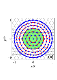
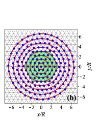
Figure 1: (Color online) Structure of equilibrium configurations for the disk geometry (a) and for the circular parabolic potential (b) for $n=187$. In both systems there are internal (core) rings corresponding to the CHL (green region). Each shell in the core contains a family of circles with radii $R_{k\ell}$ and particle numbers $n_{\rm ring}=6\,p$ (see text). The numerical solution of Eqs. (16), (42) (rings) are compared with the MD results (dots). The calculated energies ${\cal E}_{\rm avg}=23652.9/6099.5$ for disk/parabolic potentials are in a remarkable agreement with the corresponding MD results ${\cal E}_{\rm MD}=23652.2/6098.8$. The core region with ${\{\bf 1},{\bf 6},{\bf 12},{\bf 18},({\bf 24})\}$ particles, exhibits a hexagonal pattern. The valence shells contain $87,37,26$ and $34,34,34,24$ particles with an almost perfect circular structure for the disk geometry and the circular parabolic potential, respectively.

This fact can be understood by considering the arrangement of the CHC points, $\vec{x}_{k,\ell}=k\vec{a}_{1}+\ell\vec{a}_{2}$, given by integers $k,\ell$ and the two primitive Bravais lattice vectors $\vec{a}_{1}=a\,(1,0)$ and $\vec{a}_{2}=a\,(1/2,\sqrt{3}/2)$, where $a$ is the lattice constant. The $n_{p}=6\,p$ sites in the $p\!-\!{\rm th}$ shell are organised in different circular rings with radii $R_{k\ell}=a\,\sqrt{k^{2}+\ell^{2}+k\,\ell}$, where $p=k+\ell$ and $0\leq\ell\leq k$, containing either 6 (if $\ell=0,k$) or 12 (otherwise) particles (see Fig.1a). Up to $p=7$ all these radii are well ordered within and between successive shells, and the model we presented groups them in a single circular shell $n_{\rm ring}=6\,p$. Beyond the seventh shell, however, rings start to overlap (e.g., $R_{7,0}>R_{4,4}$), ultimately distorting this sequence as they depart from the centre. In other words, the CHC becomes broken giving up the reflection symmetry. The comparison of the equilibrium energies and configurations, calculated by means of our semi-analytical model and the MD, can be found in Ref. sup, . We return to this point in Sec.IVB.

The systematic manifestation of the CHL with the increase of particle number $n\geq 187$ can be interpreted as the onset of the centered hexagonal crystallization in the disk geometry. We recall that for infinite systems the hexagonal lattice has the lowest energy of all two-dimensional Wigner Bravais crystals mar . However, in our finite system a crossover takes place from a centered hexagonal lattice to ring localization at large $n$ with the approaching to disk boundary.

Thus, we have found a cyclic self-organization for finite number of charged particles confined in a disk geometry (cf. Refs. pet2, ; mug, ). For centered configurations particles localize in shells, where each $p\!-\!{\rm th}$ internal shell consists in particles distributed over a regular hexagon which is delimited by inscribed and circumscribed rings. This CHC pattern is replaced by a ring organization when approaching the boundary. A natural question arises: how general is this type of organization? Does one find a similar self-organization for other types of circular confinement? As a next example, we consider charged particles confined by an external parabolic potential.

III.2 Parabolic potential

In the case of a circular parabolic potential (3) the Hamiltonian (1) obeys a scaling law. We can express the energy and the coordinates in the following units

$$R=\left(\frac{\alpha}{\beta}\right)^{1/3}\,,\quad e_{0}=\alpha^{2/3}\beta^{1/3}\,,\quad\beta=m\omega_{0}^{2}\,,$$ (39)

where $\alpha=e^{2}/4\pi\varepsilon_{0}\varepsilon_{r}$. In such units the Hamitonian (1) can be written in the following form

$${\cal H}=\frac{H}{e_{0}}=\frac{1}{2}\sum_{i=1}^{n}x_{i}^{2}+\sum_{i<j}^{n}\frac{1}{|\vec{x}_{i}-\vec{x}_{j}|}\,,$$ (40)

where $\vec{x}_{i}=\vec{r}_{i}/R$. In the form (40) the Hamiltonian does not depend on a particular value of the confinement frequency $\omega_{0}$ or the interaction strength $\alpha>0$. Therefore, the following analysis describes universal properties for this confining potential.

III.2.1 Structure of magic configurations

To compare the results of our model with those already obtained in the disk geometry, we also neglect the energy fluctuating term in Eq. (8). Here, we consider the ground-state configurations for $n\leq 200$ (see details in Ref. sup, ). In contrast to the disk geometry, we are forced to find the maximal radius $r_{1}$ as a function of the particle number. In the scaled variables, within our approximation, we have for the total energy

$${\cal E}_{\rm avg}^{S}={\cal E}_{\rm avg}({\bf{n},\bf{x}})+\frac{1}{2}\mbox{$\sum\limits_{i=1}^{p}$}\,n_{i}x_{i}{{}^{2}}\,.$$ (41)

Here, the function ${\cal E}_{\rm avg}({\bf{n},\bf{x}})$ is defined by Eq. (15), where $r_{i}$ is replaced by $x_{i}=r_{i}/R\,,x_{i}>x_{i+1}$. We also introduce the index ”S” associated with the parabolic (soft) potential. The minimal energy configurations are obtained from the solution of the system of equations

$${\cal F}_{i}^{S}={\cal F}_{i}+\frac{\pi}{2}x_{i}^{2}=0\,,\qquad i=1,\ldots,p\,,$$ (42)

where ${\cal F}_{i}$ is determined by Eq. (III.1) with $r_{i}$ replaced by $x_{i}=r_{i}/R$.

The numerical results determine the ”magic configurations” with complete $p$ shells. The structures of these configurations are different from those of the hard-wall potential:

$$\begin{array}[]{ccccccccccc}5:&5\\ 15:&5&10\\ 32:&5&11&16\\ 52:&5&11&16&20\\ 79:&5&11&17&22&24\\ 111:&5&11&17&22&27&29\\ 148:&5&11&17&22&28&32&33\\ 190:&5&11&17&23&28&33&36&37\end{array}$$ (51)

This difference manifests also in the number of rings for the same total number of particles, $n$. Our results yield the following approximate formula for the number of shells

$$p_{S}\simeq[\sqrt{n/2}-1]\,.$$ (52)

Compared to the hard-wall potential, there are more rings in the parabolic confinement (see also Fig. 1). Nevertheless, similar to the disk potential, the addition of one electron starts developing the CHC, with internal shell occupations $6\,p$, $p=1,2,3...$. In contrast to the hard-wall case, the onset of this $6\,p$ rule is slightly delayed after the beginning of each new shell. This is reflected in the following results

$$\begin{array}[]{ccccccccccc}6:&1&5\\ 17:&{\bf 1}&{\bf 6}&10\\ 35:&{\bf 1}&{\bf 6}&{\bf 12}&16\\ 56:&{\bf 1}&{\bf 6}&{\bf 12}&17&20\\ 84:&{\bf 1}&{\bf 6}&{\bf 12}&{\bf 18}&22&25\\ 116:&{\bf 1}&{\bf 6}&{\bf 12}&{\bf 18}&23&27&29\\ 155:&{\bf 1}&{\bf 6}&{\bf 12}&{\bf 18}&{\bf 24}&28&32&34\\ 198:&{\bf 1}&{\bf 6}&{\bf 12}&{\bf 18}&{\bf 24}&29&33&37&38\\ \end{array}$$ (61)

Note that, due to the increase in energy caused by the parabolic potential, less particles are located in this case on the rings close to the boundary. In fact the corresponding scaling for the outer shell occupations are

$$n_{1}^{H} = \Big{[}2.795\,n^{2/3}-3.184\Big{]}\,,$$ (62)

$$n_{1}^{S} = \Big{[}0.2423\,n^{2/3}+6.229\,n^{1/3}-6.375\Big{]}\,.$$

These values are obtained from the fitting of the results at the range $n=2-400(300)$ for the hard wall (parabolic) potential. The analysis of this systematic data for the hard wall confinement also indicates that occupations for subsequent shells are quite accurately predicted ($\pm 1$) by our model. In particular, the second shell occupation is fitted by

$$n_{2}^{H}=\Big{[}1.351\,n^{2/3}-6.566\Big{]}.$$ (63)

In the disk geometry the energy minimization distributes a large part of particles over the perfect circular boundary. This group of charges stipulate the intrinsic ring organization in this geometry. Considering the same number of particles and system size ($r^{S}_{\rm ext}=r^{H}_{\rm ext}$), in the parabolic confinement, obviously $E^{S}_{\rm Coul}>E^{H}_{\rm Coul}$ since the equilibrium configuration $({\bf{n}},\,{\bf{r}})_{H}$ is the one that minimizes Coulomb energy. Moreover, as a consequence of the virial theorem ($E^{S}_{\rm Coul}=2\,E_{\rm HO}$), the total energy $E^{S}=3\,E^{S}_{\rm Coul}/2$ is also bigger. In order to distribute the larger amount of energy in this case the system requires additional shells, absent in the disk geometry, to equilibrate the configuration. As a consequence, in the parabolic confinement the distribution of particles over rings is less inhomogeneous as compared to the disk geometry (see also Fig. 1). In turn, this feature favours the formation of a more extended CHL.

In general, the increase of particle number in a new shell disintegrates slowly the CHL in both systems. As soon as a particle appears at the center, it gives rise to the CHL again. Below, for the sake of discussion we name our semi-analytical approach as the circular model (CM).

IV Molecular dynamics

IV.1 Basic approach

To test our results, we consider in the following both harmonic $V_{\rm ext}(r)=1/2\,m\,\omega_{0}^{2}\,r^{2}$ and hard-wall $V_{\rm ext}(r)=\infty\Theta(r-R)$ confinements. Finding the absolute energy minimum, $E_{\rm gs}$ of the Hamiltonian (1) is a non trivial task. The density of stable states near $E_{\rm gs}$ grows exponentially with the number of charges. Several global optimization techniques have been extensively used to this aim. Metropolis simulated annealing, with temperature $T$ as a control parameter, is particularly effective for short range forces. This method works on the basis of acceptance/rejection of a proposed change in the particle positions (and corresponding change in energy $\Delta E$) with probability $p(\Delta E)=\exp(-\Delta E/k_{\rm B}\,T)$. Random small changes over a single particle at a time are needed in order to guarantee a reasonable acceptance ratio, $r$. Usual practice adjusts the maximum change at any given $T$ as to have $r\sim 1/2$.

In our pursuit of the exact ground state configurations we have used a different approach, based on a quenched molecular dynamics algorithm. The method evolves the particle positions by integrating the equations of motion for the Hamiltonian (1) and adding a friction term which provides a controllable and smooth quenching of velocities

$$m\,\vec{r}_{i}^{\ {}^{\prime\prime}}=-\nabla_{i}\,V(\vec{r}_{i})-b_{\rm f}\,\vec{r}_{i}^{\ {}^{\prime}}\,.$$ (64)

Here $V(\vec{r}_{i})=V_{\rm ext}(r_{i})+\alpha\,\sum_{j\neq i}1/r_{i\,j}$ includes the external potential plus the Coulomb terms, and $b_{\rm f}$ is the parameter controlling the quenching of velocities. Below we discuss in detail our MD approach, using the circular parabolic potential as an example. A few results of the MD calculations for disk are presented in Refs. cnp, ; toni, ; sup, .

With the aid of the units (39), writing $\vec{r}=R\,\vec{x},\ E=e_{0}\,{\cal E}_{\rm MD}$ and $t=\tau/\omega_{0}$, the dynamical equations become independent of the scaling parameters for the harmonic potential

$$\ddot{\vec{x}}_{i}=-\vec{x}_{i}+\sum_{j\neq i}^{N}\frac{\vec{x}_{i}-\vec{x}_{j}}{|\vec{x}_{i}-\vec{x}_{j}|^{3}}-\nu_{\rm f}\,\dot{\vec{x}}_{i}\,,$$ (65)

where $\dot{f}\equiv df/d\tau$ and $\nu_{\rm f}$ is the scaled friction parameter. Given initial positions, the system (65) is evolved by standard centered 3-point derivative formulas, until forces over each particle are within a tolerance value (typically $|\ddot{\vec{x}}_{i}|<10^{-6}$). An advantage of this method over the Metropolis algorithm is that it produces a sensible global move at each iteration, thus requiring less simulation time. The performance of this method for obtaining ground state configurations is better than with usual Monte Carlo simulations, provided a sufficient number of initial conditions are tried. In fact, one of the common errors when using any of these algorithms is to be short in the number of trials and getting as a result an excited state configuration. To avoid as much as possible this scenario, we have included a systematic search of the $n$-particle configuration based on the lowest energy results for $n\!-\!1$ particles. For each of these configurations, the new particle is placed at different random positions. The new distinct configurations for the $n$ system are stored and ordered in energy to be used as starting points for the $n\!+\!1$ system. This strategy is suitable for a systematic search of ground state configurations in an ascending chain of $n$ charge particles.

IV.2 Search strategy for a single case

In the case of a single (large) $n$ confined system, the lowest lying energy results of the circular model, with much less degrees of freedom, provide a convenient way to feed the MD analysis with sensible initial guesses. To prove this point, we have computed the probability distribution of the energy states for $n=317$ charges confined in the disk geometry with three different types of initialization. In all cases the outer shell occupation has been fixed to $n_{1}^{H}=126$ predicted by Eq. (62). In fact, this value corresponds to the actual value associated with the MD absolute energy minimum.

As it is demonstrated in Ref. toni, , there is a remarkable agreement between the CM and MD occupations even for a charge number of subsequent shells. Hence, we aim to assess the effectiveness of the CM prediction for $n_{2}^{H}$, Eq.(63), as a guide to initialize the external particle positions in the MD. To this end we have considered initial configurations characterized by external occupations: $n_{1}=126$ (Set 1); $n_{1}=126,\,n_{2}=55$ (Set 2); $n_{1}=126,\,n_{2}=56$ (Set 3). We have generated 3650, 2000 and 2000 configurations, respectively. In each case $n_{1}$ particles were initially set on the boundary at $r_{1}=1$, and for the last two sets $n_{2}$ particles have been homogeneously distributed at $r_{2}=0.96$.

In order to preserve these external shell occupations the $n_{1},(n_{2})$, particles are frozen at a first stage, until the inner particles slow down (typically after some $500$ time steps). At a second stage, all particles are taken into account and evolved according to Eq. (65). It is worth noticing that the chosen value $r_{2}=0.96$ is higher than the CM result ($r_{2}\simeq 0.91$). The reason is twofold: i) it guarantees the desired $n_{2}$ value for the equilibrated final configuration; ii) at the beginning of the second stage it provides additional excitation energy in the form of monopole oscillations that help to access low energy states. The remaining particles are initialized randomly in the central region.

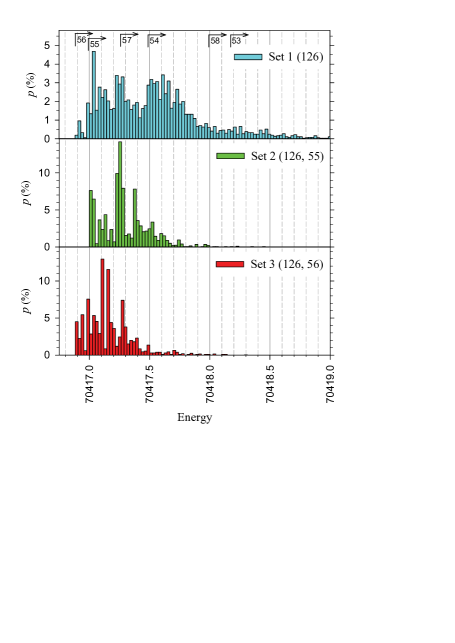
Figure 2: (Color online) Histograms for energy states of $n=317$ charges confined in the disk geometry. The results are obtained with the aid of the MD method by using different initialization procedures. See text for details.

The results for the Set 1 (see Fig. 2, top panel) consists of different final configurations with $n_{2}=53(5\%),54(36\%),55(38\%),56(18\%),57(3\%)$ and $58(0.2\%)$. The arrows indicate the starting energy for each $n_{2}$ value. In this case the low energy states are dominated by configurations with $n_{2}=(55,\,56)$, although just about one out of five runs leads to the $n_{2}$ value shared by the ground state at ${\cal E}_{\rm MD}=70416.883$. The realization of the ground state does not exceed $0.2\%$. The Set 2 (Fig. 2, middle panel) provides the lowest state ${\cal E}_{\rm MD}=70417.000$ with $n_{2}=55$ (the CM partition), which is slightly above the true ground state. The Set 3 (Fig. 2, bottom panel) explores the nearby $n_{2}=56$ configurations, with $n_{2}=n_{2}^{H}$ provided by Eq.(63). In this case the absolute energy minimum is found with a probability $\sim 4.5\%$ which is higher by a factor 25 relative to the probability found for the Set 1. Thus, even if one has to check nearby $n_{2}^{H}\pm 1$ values, the scanning effort clearly benefits from the scalings found within the CM.

For the sake of illustration, we present in Fig. 3 the distribution of charges in the equilibrium configuration obtained by means of our procedure for $n=317$. Three regions are found (see Fig. 3a). The central region (green colored hexagonal area) is comprised of the almost perfect CHL with 1,6 and 12 particles followed by a third shell containing 19 (instead of 18) particles. This additional charge (at the center of the small yellow circle) breaks the hexagonal structure. Its effect propagates to the middle region. Here, together with additional defects, it builds still a hexagonal, although deformed, structure (gray lines are used to indicate the deformed lattice). The last region contains three external rings with 126,56,42 particles. Applying a simple clustering algorithm, that will be discussed below, we can identify circular shells in the MD results (see Fig. 3b). As a result, we obtain the following configuration (126,56,42,33,22,19,12,6,1) compatible with the CM result (126,55,42,32,25,18,12,6,1) (see also sup ).

Below, we compare the MD and the CM results in more details.

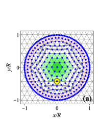
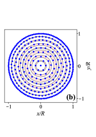
Figure 3: (Color online) Structure of equilibrium configurations for the disk geometry obtained by means of the MD for $n=317$. (a) Distribution of particles versus hexagonal grid. The core (green) region with ${\{\bf 1},{\bf 6},{\bf 12}$) particles exhibits a hexagonal pattern. The additional particle (displayed within the small yellow circle) in the third shell breaks the hexagonal $6\,p$ rule. The intermediate region can still be associated with a deformed hexagonal lattice (gray lines to guide the eye). The valence shells contain $126,56,42$ charges with an almost perfect circular structure. (b) Distribution of particles on various rings, found with the clustering algorithm described in Sec.  IV.C, with number of charges: 126,55,42,32,25,18,12,6,1.

IV.3 Molecular dynamics and the circular model

The numerical solution of the system (15),​​ (III.1) for the hard confinement provides a remarkable agreement with the MD calculations for equilibrium configurations up to $n\!=\!105$, excluding a few cases (see Table I in Ref. cnp, ). Our MD results agree with those of Ref. wor, up to $n\!=\!160$ particles, while we obtain lower energies for $n\!=\!400,500,1000$ and also systematically better values for $n>52$ than those implied in Fig. 8 of Ref. mug, . In Ref. toni, the reader can find the comparison of the MD and the CM results for the disk geometry for $161\leq n\leq 260$. In that paper, we have also demonstrated the usefulness of the CM to speed up the random search method of the true ground state for $n=395$ in the MD calculations, found in Ref.am .

Table 1: Values for the only eleven cases where optimal configurations, obtained with the aid of Eq. (42), disagree with the MD results. The systematic MD results for $n\leq 52$ can be found also in Ref.pet1 .

$n$	${{\cal E}^{S}}_{\rm avg}(n)$	$\delta$	configuration
19	115.1127	0.0208	$(11,7,1)_{2}^{1}$
22	149.7743	0.0571	$(13,8,1)_{1}^{3}$
32	290.7905	0.0655	$(16,11,5,0)_{1}^{4}$
34	323.4146	0.0537	$(16,11,6,1)_{1}^{2}$
36	357.5053	0.0313	$(16,12,7,1)_{3}^{1}$
39	411.3570	0.0392	$(18,13,7,1)_{1}^{4}$
40	430.0216	0.0924	$(18,13,8,1)_{1}^{4}$
41	449.0085	0.1290	$(18,13,8,2)_{1}^{2}$
46	548.6758	0.0976	$(18,15,9,4)_{4}^{1}$
52	678.9715	0.0671	$(20,16,11,5,0)_{1,2}^{4,5}$
53	701.8207	0.1162	$(19,16,11,6,1)_{1}^{2}$

In the case of the parabolic potential we obtain good agreement with the MD results as well, excluding a few cases (see Table 1) up to $n\approx 51$. The difference $\delta={{\cal E}^{S}}_{\rm avg}-{\cal E}_{\rm MD}$ provides the error of our approximation. The rings are counted starting from the external one which is the first ring. The notation $(11,7,1)_{2}^{1}$ means that we have to add one particle in the first ring and remove one particle from the second ring in order to obtain the MD result. Although the total energy errors are very small, the assumptions of our model fail to predict the correct configurations for shown total $n$.

Since in the disk geometry the external radius is fixed ($R=1$), the parabolic potential has one more degree of freedom in terms of collective variables. It is natural to assume that this degree of freedom is related to fluctuations of the external ring radius around some equilibrium radius value (radial fluctuations). As a result, such a motion creates fluctuations in the particle number around some optimal value in the external ring affecting the particle number in the closest ring.

In order to get deeper insight into this phenomenon we have applied a simple clustering algorithm to identify the formation of circular shells in the MD results. At a first stage, we order particles according to their distance to the centre $r_{1}\leq r_{2}\leq\cdots\leq r_{n}$. Next, we define the gaps between consecutive particles $\delta_{i}=r_{i+1}-r_{i}$ and sort them by decreasing value, i.e., $\delta_{i_{1}}\geq\delta_{i_{2}}\geq\cdots\geq\delta_{i_{n-1}}$. By defining the function

$$F_{\rm MD}(p)=\frac{r_{1}+\sum_{k=1}^{p-1}\delta_{i_{k}}}{p}\,,$$ (66)

the optimal groups are found by maximizing the average spatial separation between consecutive groups with respect to the number of shells $p$. Additionally, we impose the constraint $0\leq p(n)-p(n-1)\leq 1$ and detect when a new particle settles at the centre of the structure, $r_{1}\simeq 0$, thus opening a new shell. Once the number of shells is obtained, the related function

$$R_{\rm MD}(n)=\frac{p\,F_{\rm MD}(p)}{r_{n}}$$ (67)

provides a simple measure of how close the MD particle configuration is to a well defined ring structure. Notice that for strict circular configurations, such as those provided by our circular model, $R_{\rm MD}(n)=1$. A significant departure from this maximum value would imply that the particle distribution deviates from the prediction of the CM.

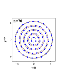
Figure 4: (Color online) Structure of the MD equilibrium configurations for $n=70,71$ charged particles in the circular parabolic potential. In both systems five rings are identified. For $n=70$ the MD configuration is ${\{\bf 3},{\bf 9},{\bf 15},{\bf 20},{\bf 23}\}$, ${\cal E}_{\rm MD}=1135.298$. The circular model predicts the same configuration with ${\cal E}_{\rm avg}^{S}=1135.474$. For $n=71$ the MD (the circular model) configuration is ${\{\bf 4},{\bf 10},{\bf 15},{\bf 21},{\bf 21}\}$ $({\{\bf 4},{\bf 9},{\bf 15},{\bf 20},{\bf 23}\})$, ${\cal E}_{\rm MD}({\cal E}_{\rm avg}^{S})=1163.410\,(1163.579)$.

This fact is illustrated in Fig. 4 where the result of this clustering algorithm is shown for $n=70,71$. The actual values $R_{\rm MD}(70)=0.775$ and $R_{\rm MD}(71)=0.520$ indicate that the system with $n=70$ is quite well described by a ring structure. It is not the case, however, for $n=71$, where the resulting shells have much larger widths. The addition of one particle produces a visible finite size effect which transforms the system from a rigid ring organization to a kind of glasslike behavior. In Fig. 5 the function (67) shows that the MD configurations form a robust circular structure for the disk geometry; its value remains close to the maximum $(\geq 90\%)$ for $n\leq 100$ charged particles. The accumulation of a big fraction of particles on the perfect circular boundary strongly constrains the internal ring organization. In this case the circular model provides a remarkable agreement with the MD results both for the equilibrium configurations and their energies.

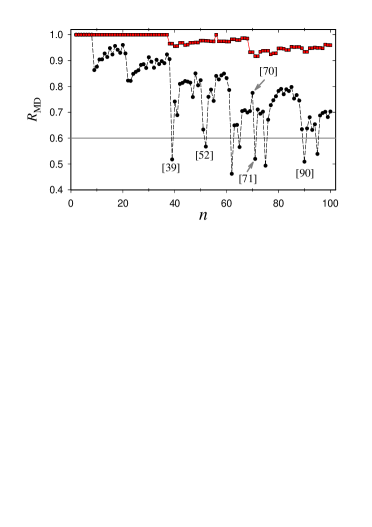
Figure 5: (Color online) The function (67) vs number of charged particles. The results for the disk geometry and the parabolic potential are shown by (red) squares and (black) circles. The arrows indicate the location of $n=70,71$ charge particle configurations discussed on Fig.4.

Conversely, while this function does frequently not drop down below $(\simeq 60\%)$ in the case of the parabolic potential, there are a few cases $n=39,52,62,65,71,75,90...$ that exhibit a visible deviation from a circular distribution. In these cases the system manifests detectable fluctuations in particle positions, driven by a change in the central structure ($n_{p}\!=\!1\to 2\ {\rm or}\ n_{p}\!>\!1\to 1$), that affect the width of the corresponding shells. In general, one observes a kind of cold melting of the system configuration that preserves, however, to some extent the ring structure.

A comparison of the MD results with those of the circular model for the total energy demonstrates a remarkable agreement. Although there is a small disagreement between the results obtained within our model and MD calculations for the ground state configurations, it is noteworthy that the onset of the centered hexagonal lattice in the MD calculations for large $n$ has been clearly recognized with the aid of the circular model.

V Summary

We have developed the method (see Sects. II, III) which allows us to analyze the equilibrium formation and filling of rings with a finite number of particles interacting by means of the Coulomb forces in the case of a circular lateral confinement. As an example, we analyzed disk and parabolic confinements. Our approach is based on the cyclic symmetry of the Coulomb energy between particles distributed over different rings. As a result, the problem of $n$ interacting charged particles is reduced to the description of $p\,(\ll\!\!n)$ rings, with homogeneously distributed integer charges. To test the validity of the method we have also developed the MD approach (Sec. IV) and present the comparison of the results in Ref. sup, .

We have demonstrated that our method is good enough to obtain exact ground state configurations with correct energies, excluding a few particular cases, up to $n\leq\!105$ and $\leq\!51$ for a hard and parabolic confinements, respectively. For bigger systems the solution of the model equations provide also very good approximations to the exact ground state configurations. Indeed, the energy errors do not exceed a small percentage fraction of the exact values. However, this achievement is a necessary but not a sufficient condition to conclude that the CM is effective. The systematic analysis of the CM results provides the estimate for a number of charges $n_{1}$ distributed over the external (boundary) ring for large systems $(n\leq 400)$. Once this number is identified, one has to fix the number of charges on the second ring, the nearest neighbor to the boundary one, based on the CM prediction $n_{2}\pm 1$. At the same time, the inner shell structure, as predicted by the CM, should be disregaded, since it may introduce a bias. With the aid of this strategy the computational effort to get global energy minima is much less than in the MD or simulated annealing (SA) calculations. In fact, both methods are flawed by two major problems. First, due to the long range of Coulomb forces, computing time grows with the number of particles as $n^{3}$. Second, and more important, the number of equilibrium configurations near the absolute energy minimum grows exponentially with $n$. This last fact increases considerably the computational efforts needed to avoid getting stuck at local energy minima, because many different initial condition simulations are needed. Therefore, we believe that an accurate method, capable of explaining shell structure, which works with a much reduced number of variables ($\sqrt{n/2}$ vs $n$) is a remarkable achievement. Moreover, the results obtained by means of our method can be used to feed SA or MD calculations with sensible initial configurations, reducing substantially the amount of scanning normally needed to visit the global energy minima.

In our circular model each $p\!-\!{\rm th}$ shell consists of a set of point charges distributed over a regular hexagon inscribed and circumscribed by two circles. Based on the results of our analysis, we have found that in both potentials the increase of particle number leads to the onset of a centered hexagonal lattice that transforms smoothly to a few circular rings at the boundary. A similar conclusion has been drawn on the basis of the Monte Carlo calculations for $n>150$ charges confined by a circular parabolic potential pet3 , although the authors admitted that their equilibrium configurations are not necessarily true ground states. Based on our results we speculate that this self-organization should be typical for any 2D finite system of identical charges confined by a circularly symmetric potential. We recall, however, that depending on the size of the system one has to take into account the onset of quantum correlations for increasing particle number at a fixed system size (see a discussion in Ref. cnp, ).

Appendix A Cyclic symmetry and the Coulomb sums

We want to prove that

$$\sum_{i=1}^{n}\sum_{j=1}^{m}\,\textrm{F}\!\left[\cos\left(2\pi\left(\frac{i}{n}-\frac{j}{m}\right)\right)\right]=G\,\sum_{k=1}^{L}\,\textrm{F}\!\left[\cos\left(2\pi\frac{k}{L}\right)\right]\ ,$$

where $L\equiv{\rm LCM}(n,m)$ and $G\equiv{\rm GCD}(n,m)=n\times m/L$ are the least common multiple and greatest common divisor of the of numbers $(n,m)$, respectively.

Proof:

Due to the fact that F is a function (every element belonging to the domain is related to a unique element of the image set) it suffices to prove that the multiset of angles $A=\Bigl{\{}2\pi\left(\frac{i}{n}-\frac{j}{m}\right),\;i=1,\ldots,n\,\wedge\,j=1,\ldots,m\Bigr{\}}$ is equal, under the cyclic symmetry, to the multiset $B=\Bigl{\{}2\pi\frac{k}{L}\,,k=1\ldots L\Bigr{\}}$, where each element is repeated $G$ times.

In order to take into account the cyclic symmetry explicitly, we change the numbers $k$ by their associated equivalence classes, defined as $C_{k}=\Bigl{\{}k+\gamma\mspace{1.0mu}L\,,\>\forall\,\gamma\in\mathbb{Z}\Bigr{\}}$. As a result, a $k$-value appearing inside the $B$ multiset has to be read as an unspecified member of the $C_{k}$ class. The set composed by all these classes constitutes a partition of $\mathbb{Z}$ into $L$ classes.

Since any linear combination of two integers $(n,m)$ is equal to a multiple of its greatest common divisor $G={\rm GCD}(n,m)$, we have

$$\frac{i}{n}-\frac{j}{m}=\frac{i\mspace{1.0mu}m-j\mspace{1.0mu}n}{n\mspace{1.0mu}m}=\frac{k\mspace{1.0mu}G}{n\mspace{1.0mu}m}=\frac{k\mspace{1.0mu}G}{L\mspace{1.0mu}G}=\frac{k}{L}\,,$$ (68)

where $k$ is an integer. Evidently, this result allows us to change two sums over the variables $i$ and $j$ by a single suitable sum over the variable $k$.

Note that for the multiset of angles $A$ the substitutions

$$i\rightarrow i+\alpha\mspace{1.0mu}n j\rightarrow j+\beta\mspace{1.0mu}m\ ,$$ and

where $\alpha,\beta\in\mathbb{Z}$, have no practical effect. Furthermore, since a pair of indices $(i,j)$ produces an index $k$ that belongs to the class $C_{k}$, the shifted pair of indices $(i+\alpha\mspace{1.0mu}n,j+\beta\mspace{1.0mu}m)$ produces an index $k^{\prime}$ that also belongs to the class $C_{k}$:

$$(i+\alpha\mspace{1.0mu}n)\mspace{1.0mu}m-(j+\beta\mspace{1.0mu}m)\mspace{1.0mu}n=i\mspace{1.0mu}m-j\mspace{1.0mu}n+(\alpha-\beta)\mspace{1.0mu}L\mspace{1.0mu}G=$$

$$(k+(\alpha-\beta)\mspace{1.0mu}L)\mspace{1.0mu}G\,.$$

Evidently, there are exactly $L$ different $C_{k}$ classes.

Now we show that each class contains G different elements. If there exists a pair $(i,j)$ such that

$$i\mspace{1.0mu}m-j\mspace{1.0mu}n=k\mspace{1.0mu}G\,,$$ (69)

then there are exactly $G$ pairs $(i^{\prime},j^{\prime})$, with the restrictions $1\leq i^{\prime}\leq n$ and $1\leq j^{\prime}\leq m$, such that $i^{\prime}\mspace{1.0mu}m-j^{\prime}\mspace{1.0mu}n=k\mspace{1.0mu}G$. Note that if $(i,j)$ satisfy (69), then all couples of the form

$$\left(i^{\prime}=i+l\mspace{1.0mu}\frac{n}{G}\>,\,j^{\prime}=j+l\mspace{1.0mu}\frac{m}{G}\right)\;,$$

where $l$ is an arbitrary integer, also satisfy  (69), because

$$i^{\prime}\mspace{1.0mu}m-j^{\prime}\mspace{1.0mu}n=\left(i+l\mspace{1.0mu}\frac{n}{G}\right)m-\left(j+l\mspace{1.0mu}\frac{m}{G}\right)n=i\mspace{1.0mu}m-j\mspace{1.0mu}n=k\mspace{1.0mu}G\;.$$

If we restrict the values of $l$ to $0\leq l\leq G-1$, i.e. $G$ different choices, the resulting values $i^{\prime}$ and $j^{\prime}$ are all different. Indeed, in this situation, if $G>1$, the following inequalities hold

$$\frac{n}{G}\leq|i^{\prime}-i^{\prime\prime}|<n \frac{m}{G}\leq|j^{\prime}-j^{\prime\prime}|<m\ .$$ and

If $l=G+\lambda$, with $\lambda=0,1,2,\ldots$ the indices are cyclicly equivalent

$$i+\frac{(G+\lambda)\mspace{1.0mu}n}{G}=i+n+\frac{\lambda\mspace{1.0mu}n}{G}\sim i+\frac{\lambda\mspace{1.0mu}n}{G}\;.$$

Therefore, since there are $n\mspace{1.0mu}m$ pairs, every one of the $L$ different $C_{k}$ classes must contain $G$ pairs. This completes the proof. The fact that we consider a cosine function is irrelevant, since the requirement that $\epsilon(r_{1},r_{2},\theta)$ to be periodic is enough.

Appendix B Coefficients of the Fourier transform

In order to find an analytical expression for the integral (11), we employ the Legendre expansion for the Coulomb potential

$$\frac{1}{\left[r_{1}^{2}+r_{2}^{2}-2\,r_{1}\,r_{2}\,\cos\psi\right]^{1/2}}=\frac{1}{r_{>}}\sum_{u=0}^{\infty}t^{u}P_{u}(\cos\psi)\,,$$

where $r_{>}=\max(r_{1},r_{2})$, $r_{<}=\min(r_{1},r_{2})$, $t=r_{<}/r_{>}$. With the aid of the cosine series for the Legendre polynomials (see Ref. AS, , p. 776)

$$P_{u}(\cos\psi)=\frac{1}{4^{u}}\sum_{v=0}^{u}\binom{2v}{v}\binom{2(u-v)}{u-v}\cos\left((u-2v)\psi\right)\,,$$

we obtain for Eq. (11) the following form

$$C_{\ell nm}(r_{1},r_{2}) = \frac{nm}{r_{>}\pi}\sum_{v=0}^{\infty}\left(\frac{t}{4}\right)^{v}\binom{2v}{v}\sum_{w=0}^{v}\left(\frac{t}{4}\right)^{w}\binom{2w}{w}$$ (70)

$$\times \int_{0}^{2\pi}\cos\left[(w-v)\psi\right]\cos(\ell L\psi)\,d\psi\,,$$

where $u=w+v$. The integral splits in two terms, since $\cos A\cos B=\left[\cos(A+B)+\cos(A-B)\right]/2$. In order to have a nonzero value, the first term with the argument $w=v-lL$ in the cosine function requires $v\geq lL$. As a result, we have

$$C_{\ell nm}(r_{1},r_{2})=\frac{nm}{r_{>}}\sum_{v=\ell L}^{\infty}\left(\frac{t}{4}\right)^{2v-\ell L}\binom{2v}{v}\binom{2(v-\ell L)}{v-\ell L}$$

$$=\frac{nm}{r_{>}}\left(\frac{t}{4}\right)^{\ell L}\sum_{k=0}^{\infty}\binom{2(\ell L+k)}{\ell L+k}\binom{2k}{k}\,\left(\frac{t}{4}\right)^{2k}\,,$$ (71)

where $k=v-\ell L$. The second term yields the same result, that duplicates the expression (71).

This double sum can be expressed in terms of the hypergeometric function. In virtue of the identity

$$\frac{1}{4^{p}}=\frac{\Gamma(p+1/2)}{\sqrt{\pi}{p!}}\,,$$

we arrive at the final form

$$C \!\!\!\!{}_{\ell nm}(r_{1},r_{2})=$$ (72)

$$= \frac{2nm}{r_{>}}\,\frac{t^{\ell L}}{\pi}\,\sum_{k=0}^{\infty}\frac{\Gamma(\ell L+k+1/2)\Gamma(k+1/2)}{\Gamma(\ell L+k+1)k!}t^{2k}$$

$$= \frac{2nm}{r_{>}}\,\frac{t^{\ell L}}{\sqrt{\pi}}\,\frac{\Gamma(\ell L+1/2)}{(\ell L)!}\,\sum_{k=0}^{\infty}\frac{(1/2)_{k}(\ell L+1/2)_{k}}{(\ell L+1)_{k}}\frac{t^{2k}}{k!}$$

$$= \frac{2nm}{r_{>}}\,\frac{(2\ell L-1)!!}{(\ell L)!}\left(\frac{t}{2}\right)^{\ell L}\times$$

$$\times{}_{2}F_{\mspace{-1.0mu}1}\Bigl{(}1/2\,,\ell L+1/2\,;\ell L+1\,;\,t^{2}\Bigr{)}\,.$$

Here, we have used a definition of the hypergeometric function in terms of the Pochhammer symbol $(a)_{b}=\Gamma(a+b)/\Gamma(a)$.

At $\ell L\gg 1$ one can use the asymptotic value for the central binomial coefficients $\binom{2M}{M}/(4^{M})\approx 1/\sqrt{\pi M}$ , where $M=\ell L$. As a result, we obtain the asymptotic limit of Eq. (72):

$$C_{\ell nm}(r_{1},r_{2})\approx\frac{2nm}{\sqrt{\pi}\,r_{>}}\,\sum_{k=0}^{\infty}\frac{\binom{2k}{k}}{4^{k}}\frac{t^{\ell L+2k}}{\sqrt{\ell L+k}}\ .$$

This result shows explicitly the decreasing magnitude of the coefficients accompanying the powers of the variable $t$ in Eq. (II.2) with the increase of the product $\ell\,L$.

Supplemental Material: The MD and Circular Model results

I: Disk geometry

These tables summarize our results corresponding to the minimum energy equilibrium configurations under disk confinement, discussed in Sec.IIIA.

DATA for Table (Eq. (18))

n	CM energies	Configuration	MD energies	Configuration
11:	48.57568	[11]	48.57568	[11]
29:	444.5491	[23,6]	444.5478	[23,6]
55:	1792.007	[37,13,5]	1791.974	[37,13,5]
90:	5115.563	[53,20,12,5]	5115.408	[52,20,12,5,1]
135:	11995.371	[70,29,19,12,5]	11994.978	[70,28,19,12,5,1]
186:	23391.044	[87,37,26,19,12,5]	23390.284	[87,37,26,18,11,6,1]
246:	41743.132	[106,46,34,25,18,12,5]	41741.995	[106,46,34,25,16,12,6,1]
316:	69962.348	[126,56,42,32,25,18,11,5]	69960.435	[126,55,42,33,26,15,12,6,1]
394:	110093.60	[147,66,50,40,32,25,18,11,5]	110090.41	[147,66,50,40,26,26,19,13,6,1]

DATA for Table (Eq. (20))

n	CM energies	Configuration	MD energies	Configuration
12:	59.57568	[11,1]	59.57568	[11,1]
30:	479.0854	[23,6,1]	479.0796	[23,6,1]
56:	1862.734	[37,12,6,1]	1862.650	[37,12,6,1]
92:	5358.578	[53,20,12,6,1]	5358.353	[53,20,12,6,1]
136:	12181.755	[70,28,19,12,6,1]	12181.345	[70,28,19,12,6,1]
187:	23652.947	[87,37,26,18,12,6,1]	23652.188	[87,37,26,18,12,6,1]
248:	42447.440	[106,46,34,25,18,12,6,1]	42446.278	[107,46,34,25,17,12,6,1]
317:	70418.854	[126,55,42,32,25,18,12,6,1]	70416.883	[126,56,42,33,22,19,12,6,1]
395:	110667.59	[147,65,50,40,32,24,18,12,6,1]	110664.44	[147,66,51,40,26,26,19,13,6,1]

II: Parabolic confinement

These tables summarize our results corresponding to the minimum energy equilibrium configurations under parabolic confinement. $E_{\rm MD}$, $E_{\rm CM}$ are the total MD and the Circular Model energies. $R_{\rm avg}$ and $R_{\rm ext}$ are respectively the average radius for the external shell in MD and the external CM radius. All quantities are expressed in parabolic units, defined in the main text. The approximate shell configuration in MD has been obtained by the algorithm described in Sec.IVB. Notice that for specific values of $n$ (e.g., $n=90$) some intermediate shells appear grouped together, indicating rather big particle dispersions within those shells.

Results for $2\leq n\leq 33$

$n$	$E_{\rm MD}$	Configuration	$R_{\rm avg}$	$E_{\rm CM}$	Configuration	$R_{\rm ext}$
2	1.190551	[2]	0.630	1.190551	[2]	0.630
3	3.120126	[3]	0.833	3.120126	[3]	0.833
4	5.827177	[4]	0.985	5.827177	[4]	0.985
5	9.280127	[5]	1.112	9.280127	[5]	1.112
6	13.35587	[5,1]	1.334	13.35587	[5,1]	1.334
7	17.99543	[6,1]	1.414	17.99543	[6,1]	1.414
8	23.29609	[7,1]	1.490	23.29609	[7,1]	1.490
9	29.20266	[7,2]	1.640	29.24607	[7,2]	1.646
10	35.59701	[8,2]	1.699	35.63458	[8,2]	1.704
11	42.47199	[8,3]	1.830	42.50370	[8,3]	1.834
12	49.89776	[9,3]	1.877	49.93147	[9,3]	1.882
13	57.79314	[9,4]	1.992	57.81205	[9,4]	1.995
14	66.21506	[10,4]	2.033	66.23594	[10,4]	2.036
15	75.09498	[10,5]	2.134	75.10986	[10,5]	2.137
16	84.44850	[10,5,1]	2.228	84.49102	[10,5,1]	2.234
17	94.21966	[10,6,1]	2.320	94.23676	[10,6,1]	2.323
18	104.4085	[11,6,1]	2.349	104.4258	[11,6,1]	2.352
19	115.0919	[12,6,1]	2.377	115.1127	[11,7,1]	2.434
20	126.1922	[12,7,1]	2.460	126.2002	[12,7,1]	2.461
21	137.7733	[13,7,1]	2.486	137.7859	[13,7,1]	2.488
22	149.7172	[12,8,2]	2.608	149.7743	[13,8,1]	2.562
23	162.0612	[13,8,2]	2.632	162.1328	[13,8,2]	2.635
24	174.7901	[13,8,3]	2.701	174.8619	[13,8,3]	2.705
25	187.9243	[13,9,3]	2.768	187.9888	[13,9,3]	2.771
26	201.4657	[14,9,3]	2.788	201.5293	[14,9,3]	2.791
27	215.3890	[14,9,4]	2.852	215.4374	[14,9,4]	2.855
28	229.6947	[14,10,4]	2.913	229.7357	[14,10,4]	2.915
29	244.3994	[15,10,4]	2.931	244.4401	[15,10,4]	2.933
30	259.4762	[15,10,5]	2.990	259.5184	[15,10,5]	2.992
31	274.9301	[15,11,5]	3.046	274.9566	[15,11,5]	3.048
32	290.7250	[15,11,5,1]	3.101	290.7905	[16,11,5]	3.064
33	306.8574	[15,11,6,1]	3.156	306.9034	[15,11,6,1]	3.159

Results for $34\leq n\leq 77$

$n$	$E_{\rm MD}$	Configuration	$R_{\rm avg}$	$E_{\rm CM}$	Configuration	$R_{\rm ext}$
34	323.3609	[15,12,6,1]	3.206	323.4146	[16,11,6,1]	3.173
35	340.2139	[16,12,6,1]	3.221	340.2722	[16,12,6,1]	3.223
36	357.4740	[17,12,6,1]	3.235	357.5053	[16,12,7,1]	3.274
37	375.0712	[17,12,7,1]	3.286	375.0966	[17,12,7,1]	3.288
38	393.0063	[17,13,7,1]	3.334	393.0316	[17,13,7,1]	3.335
39	411.3178	[17,13,7,2]	3.379	411.3570	[18,13,7,1]	3.348
40	429.9292	[17,13,8,2]	3.428	430.0216	[18,13,8,1]	3.396
41	448.8795	[17,14,8,2]	3.470	449.0085	[18,13,8,2]	3.443
42	468.1613	[17,14,8,3]	3.517	468.2858	[17,14,8,3]	3.521
43	487.7576	[17,14,9,3]	3.560	487.8788	[17,14,9,3]	3.566
44	507.6915	[18,14,9,3]	3.573	507.7930	[18,14,9,3]	3.576
45	527.9573	[18,15,9,3]	3.613	528.0866	[18,15,9,3]	3.617
46	548.5782	[19,15,9,3]	3.624	548.6758	[18,15,9,4]	3.660
47	569.4976	[18,15,10,4]	3.697	569.5784	[18,15,10,4]	3.701
48	590.7302	[19,15,10,4]	3.708	590.8007	[19,15,10,4]	3.710
49	612.3010	[19,16,10,4]	3.746	612.3879	[19,16,10,4]	3.749
50	634.2032	[20,16,10,4]	3.756	634.2870	[20,16,10,4]	3.758
51	656.3994	[19,16,11,5]	3.822	656.4737	[19,16,11,5]	3.828
52	678.9044	[19,15,11,6,1]	3.858	678.9715	[20,16,11,5]	3.837
53	701.7045	[18,17,11,6,1]	3.920	701.8207	[19,16,11,6,1]	3.906
54	724.7968	[18,17,12,6,1]	3.957	724.9130	[20,16,11,6,1]	3.913
55	748.2062	[19,17,12,6,1]	3.969	748.3280	[20,17,11,6,1]	3.949
56	771.9241	[20,17,12,6,1]	3.981	772.0267	[20,17,12,6,1]	3.985
57	795.9622	[20,18,12,6,1]	4.014	796.0610	[21,17,12,6,1]	3.992
58	820.3013	[21,18,12,6,1]	4.023	820.4069	[21,17,12,7,1]	4.028
59	844.9824	[22,18,12,6,1]	4.031	845.0472	[21,18,12,7,1]	4.062
60	869.9167	[21,18,13,7,1]	4.094	869.9729	[21,18,13,7,1]	4.096
61	895.1684	[22,18,13,7,1]	4.101	895.2196	[22,18,13,7,1]	4.103
62	920.7048	[21,17,14,8,2]	4.155	920.7905	[22,19,13,7,1]	4.136
63	946.5161	[20,19,14,8,2]	4.212	946.6672	[22,19,13,8,1]	4.170
64	972.6175	[21,19,14,8,2]	4.222	972.7978	[22,19,14,8,1]	4.203
65	999.0138	[20,19,14,9,3]	4.270	999.2149	[22,19,14,8,2]	4.236
66	1025.691	[20,20,14,9,3]	4.305	1025.899	[22,19,14,8,3]	4.269
67	1052.661	[20,20,15,9,3]	4.338	1052.847	[22,19,14,9,3]	4.301
68	1079.908	[21,20,15,9,3]	4.345	1080.113	[23,19,14,9,3]	4.306
69	1107.457	[22,20,15,9,3]	4.354	1107.656	[23,19,15,9,3]	4.338
70	1135.298	[23,20,15,9,3]	4.363	1135.474	[23,20,15,9,3]	4.367
71	1163.410	[21,21,15,10,4]	4.429	1163.579	[23,20,15,9,4]	4.398
72	1191.798	[21,21,16,10,4]	4.465	1191.945	[23,20,15,10,4]	4.429
73	1220.463	[22,21,16,10,4]	4.472	1220.627	[23,20,16,10,4]	4.459
74	1249.421	[23,21,16,10,4]	4.481	1249.580	[24,20,16,10,4]	4.464
75	1278.653	[23,21,14,11,5,1]	4.503	1278.801	[24,21,16,10,4]	4.492
76	1308.157	[22,21,16,11,5,1]	4.554	1308.330	[24,21,16,10,5]	4.521
77	1337.925	[22,22,16,11,5,1]	4.583	1338.091	[24,21,16,11,5]	4.550

Results for $78\leq n\leq 119$

$n$	$E_{\rm MD}$	Configuration	$R_{\rm avg}$	$E_{\rm CM}$	Configuration	$R_{\rm ext}$
78	1367.963	[22,22,17,11,5,1]	4.612	1368.158	[24,21,17,11,5]	4.579
79	1398.252	[22,22,17,11,6,1]	4.640	1398.493	[24,22,17,11,5]	4.606
80	1428.827	[22,22,17,12,6,1]	4.669	1429.075	[24,21,17,11,6,1]	4.636
81	1459.672	[22,22,18,12,6,1]	4.696	1459.914	[24,21,17,12,6,1]	4.664
82	1490.795	[23,22,18,12,6,1]	4.702	1491.015	[24,22,17,12,6,1]	4.690
83	1522.175	[23,23,18,12,6,1]	4.727	1522.396	[25,22,17,12,6,1]	4.694
84	1553.845	[24,23,18,12,6,1]	4.733	1554.064	[25,22,18,12,6,1]	4.721
85	1585.785	[24,24,18,12,6,1]	4.757	1586.000	[25,22,18,12,7,1]	4.748
86	1618.019	[25,24,18,12,6,1]	4.764	1618.192	[25,23,18,12,7,1]	4.773
87	1650.497	[24,24,18,13,7,1]	4.812	1650.637	[25,23,18,13,7,1]	4.800
88	1683.217	[24,24,19,13,7,1]	4.837	1683.354	[26,23,18,13,7,1]	4.803
89	1716.199	[24,24,19,13,7,2]	4.860	1716.355	[26,23,19,13,7,1]	4.829
90	1749.437	[24,24,32,6,2,2]	4.888	1749.623	[26,24,19,13,7,1]	4.853
91	1782.929	[24,24,19,14,8,2]	4.912	1783.153	[27,24,19,13,7,1]	4.857
92	1816.674	[24,24,19,14,8,3]	4.934	1816.963	[27,24,19,14,7,1]	4.883
93	1850.697	[24,24,19,14,9,3]	4.957	1850.998	[27,24,19,14,8,1]	4.908
94	1884.964	[24,24,20,14,9,3]	4.984	1885.300	[27,24,19,14,8,2]	4.933
95	1919.486	[25,25,19,14,9,3]	4.990	1919.823	[26,24,19,14,9,3]	4.981
96	1954.254	[25,25,20,14,9,3]	5.013	1954.592	[26,24,20,14,9,3]	5.005
97	1989.285	[25,25,20,15,9,3]	5.038	1989.618	[27,24,20,14,9,3]	5.008
98	2024.569	[25,25,21,15,9,3]	5.061	2024.897	[27,24,20,15,9,3]	5.032
99	2060.131	[26,25,21,15,9,3]	5.066	2060.434	[27,25,20,15,9,3]	5.055
100	2095.931	[26,26,21,15,9,3]	5.088	2096.242	[27,25,20,15,9,4]	5.079
101	2131.979	[26,26,21,14,10,4]	5.112	2132.277	[27,25,20,15,10,4]	5.103
102	2168.273	[26,26,20,16,10,4]	5.136	2168.562	[27,25,21,15,10,4]	5.126
103	2204.812	[26,26,21,16,10,4]	5.158	2205.103	[27,25,21,16,10,4]	5.149
104	2241.601	[26,26,22,16,10,4]	5.180	2241.889	[28,25,21,16,10,4]	5.152
105	2278.670	[27,26,22,16,10,4]	5.185	2278.931	[28,26,21,16,10,4]	5.174
106	2315.960	[26,26,21,16,11,5,1]	5.222	2316.247	[29,26,21,16,10,4]	5.176
107	2353.486	[26,26,22,15,11,6,1]	5.249	2353.799	[28,26,21,16,11,5]	5.220
108	2391.253	[26,26,20,17,12,6,1]	5.273	2391.574	[28,26,22,16,11,5]	5.242
109	2429.264	[26,26,21,17,12,6,1]	5.294	2429.600	[28,26,22,17,11,5]	5.265
110	2467.525	[26,26,21,18,12,6,1]	5.315	2467.872	[29,26,22,17,11,5]	5.267
111	2506.023	[27,27,20,18,12,6,1]	5.320	2506.392	[29,27,22,17,11,5]	5.288
112	2544.754	[27,27,21,18,12,6,1]	5.341	2545.141	[28,26,22,17,12,6,1]	5.332
113	2583.739	[27,27,22,18,12,6,1]	5.361	2584.123	[28,27,22,17,12,6,1]	5.352
114	2622.965	[27,27,23,18,12,6,1]	5.382	2623.339	[29,27,22,17,12,6,1]	5.354
115	2662.432	[27,27,24,18,12,6,1]	5.402	2662.804	[29,27,23,17,12,6,1]	5.375
116	2702.166	[28,28,23,18,12,6,1]	5.406	2702.508	[29,27,23,18,12,6,1]	5.397
117	2742.111	[28,28,24,18,12,6,1]	5.426	2742.473	[30,27,23,18,12,6,1]	5.399
118	2782.346	[29,28,24,18,12,6,1]	5.430	2782.676	[30,28,23,18,12,6,1]	5.419
119	2822.794	[29,29,24,18,12,6,1]	5.449	2823.104	[29,28,23,18,13,7,1]	5.459

Results for $120\leq n\leq 160$ $n$ $E_{\rm MD}$ Configuration $R_{\rm avg}$ $E_{\rm CM}$ Configuration $R_{\rm ext}$ 120 2863.472 [28,28,24,19,12,8,1] 5.489 2863.765 [30,28,23,18,13,7,1] 5.461 121 2904.384 [28,28,41,14,6,2,2] 5.511 2904.669 [30,28,24,18,13,7,1] 5.482 122 2945.520 [28,28,25,17,14,8,2] 5.531 2945.811 [30,28,24,19,13,7,1] 5.502 123 2986.892 [28,28,25,32,6,2,2] 5.550 2987.209 [31,28,24,19,13,7,1] 5.504 124 3028.501 [28,28,42,14,6,3,3] 5.571 3028.839 [31,29,24,19,13,7,1] 5.524 125 3070.333 [29,29,25,16,14,9,3] 5.574 3070.723 [31,29,25,19,13,7,1] 5.544 126 3112.398 [29,29,22,20,14,9,3] 5.594 3112.844 [31,29,25,19,14,7,1] 5.564 127 3154.706 [29,29,25,18,14,9,3] 5.613 3155.173 [31,29,25,19,14,8,1] 5.584 128 3197.232 [29,29,23,20,15,9,3] 5.633 3197.732 [31,29,25,20,14,8,1] 5.604 129 3240.000 [29,29,24,20,15,9,3] 5.652 3240.519 [31,29,25,20,14,8,2] 5.625 130 3282.996 [29,29,24,21,15,9,3] 5.671 3283.503 [30,29,25,20,14,9,3] 5.663 131 3326.229 [29,29,25,21,15,9,3] 5.690 3326.718 [31,29,25,20,14,9,3] 5.664 132 3369.693 [29,29,26,21,15,9,3] 5.708 3370.165 [31,29,25,20,15,9,3] 5.684 133 3413.392 [30,30,26,20,15,9,3] 5.711 3413.863 [31,30,25,20,15,9,3] 5.702 134 3457.312 [30,30,26,21,15,9,3] 5.730 3457.790 [31,30,26,20,15,9,3] 5.721 135 3501.457 [30,30,24,21,16,10,4] 5.750 3501.939 [31,30,26,21,15,9,3] 5.741 136 3545.825 [30,30,27,19,16,10,4] 5.768 3546.313 [31,29,26,21,15,10,4] 5.761 137 3590.431 [30,30,27,20,16,10,4] 5.786 3590.891 [31,30,26,21,15,10,4] 5.779 138 3635.262 [30,30,26,22,16,10,4] 5.805 3635.710 [31,30,26,21,16,10,4] 5.798 139 3680.315 [30,30,27,22,16,10,4] 5.822 3680.751 [32,30,26,21,16,10,4] 5.799 140 3725.602 [30,30,28,22,16,10,4] 5.840 3726.043 [32,31,26,21,16,10,4] 5.817 141 3771.105 [30,30,2,44,17,11,6,1] 5.861 3771.558 [32,31,27,21,16,10,4] 5.835 142 3816.828 [31,31,23,22,17,11,6,1] 5.864 3817.291 [32,31,27,22,16,10,4] 5.854 143 3862.771 [30,30,26,22,17,11,6,1] 5.896 3863.253 [33,31,27,22,16,10,4] 5.855 144 3908.934 [31,31,25,22,17,11,6,1] 5.899 3909.439 [32,31,27,22,16,11,5] 5.891 145 3955.315 [30,30,26,23,17,12,6,1] 5.932 3955.833 [32,31,27,22,17,11,5] 5.909 146 4001.923 [31,31,25,23,17,12,6,1] 5.936 4002.450 [33,31,27,22,17,11,5] 5.910 147 4048.753 [31,31,25,23,18,12,6,1] 5.953 4049.312 [33,32,27,22,17,11,5] 5.927 148 4095.803 [30,30,28,23,18,12,6,1] 5.984 4096.391 [33,32,28,22,17,11,5] 5.945 149 4143.077 [31,31,26,24,18,12,6,1] 5.989 4143.661 [32,31,27,23,17,12,6,1] 5.982 150 4190.571 [30,30,29,24,18,12,6,1] 6.019 4191.146 [33,31,27,23,17,12,6,1] 5.983 151 4238.292 [31,31,28,24,18,12,6,1] 6.022 4238.852 [33,31,28,23,17,12,6,1] 6.000 152 4286.238 [32,32,27,24,18,12,6,1] 6.025 4286.779 [33,32,28,23,17,12,6,1] 6.016 153 4334.404 [32,32,28,24,18,12,6,1] 6.041 4334.920 [33,32,28,23,18,12,6,1] 6.034 154 4382.789 [32,32,29,24,18,12,6,1] 6.058 4383.304 [34,32,28,23,18,12,6,1] 6.035 155 4431.402 [32,32,30,24,18,12,6,1] 6.074 4431.919 [34,32,28,24,18,12,6,1] 6.052 156 4480.240 [33,33,29,24,18,12,6,1] 6.076 4480.739 [33,32,28,24,18,13,7,1] 6.087 157 4529.280 [33,33,30,24,18,12,6,1] 6.092 4529.763 [34,32,28,24,18,13,7,1] 6.087 158 4578.533 [31,31,53,19,14,6,2,2] 6.140 4579.002 [34,32,29,24,18,13,7,1] 6.104 159 4627.983 [32,32,30,41,14,6,2,2] 6.144 4628.461 [34,33,29,24,18,13,7,1] 6.120 160 4677.653 [32,32,53,19,14,6,2,2] 6.159 4678.133 [34,33,29,24,19,13,7,1] 6.137

Results for $161\leq n\leq 200$ $n$ $E_{\rm MD}$ Configuration $R_{\rm avg}$ $E_{\rm CM}$ Configuration $R_{\rm ext}$ 161 4727.551 [33,33,30,41,14,6,2,2] 6.163 4728.043 [35,33,29,24,19,13,7,1] 6.138 162 4777.653 [32,32,54,20,14,6,2,2] 6.192 4778.179 [35,33,29,25,19,13,7,1] 6.155 163 4827.973 [32,32,55,20,14,6,2,2] 6.208 4828.523 [35,33,30,25,19,13,7,1] 6.171 164 4878.503 [31,31,31,25,20,14,9,3] 6.237 4879.078 [35,34,30,25,19,13,7,1] 6.187 165 4929.243 [32,32,55,20,14,6,3,3] 6.241 4929.869 [36,34,30,25,19,13,7,1] 6.188 166 4980.198 [31,31,31,25,21,15,9,3] 6.270 4980.862 [35,34,30,25,19,14,8,1] 6.221 167 5031.363 [32,32,31,45,15,6,3,3] 6.274 5032.046 [35,34,30,25,20,14,8,1] 6.237 168 5082.740 [32,32,31,26,20,15,9,3] 6.288 5083.459 [35,34,30,25,20,14,8,2] 6.254 169 5134.328 [32,32,31,26,21,15,9,3] 6.305 5135.059 [34,34,30,25,20,14,9,3] 6.287 170 5186.133 [32,32,32,26,21,15,9,3] 6.320 5186.850 [35,34,30,25,20,14,9,3] 6.287 171 5238.158 [33,33,57,21,15,6,3,3] 6.323 5238.859 [35,34,30,25,20,15,9,3] 6.303 172 5290.383 [33,33,31,27,21,15,9,3] 6.338 5291.081 [35,34,30,26,20,15,9,3] 6.319 173 5342.830 [33,33,32,27,21,15,9,3] 6.354 5343.522 [35,34,31,26,20,15,9,3] 6.335 174 5395.482 [32,32,32,26,22,16,10,4] 6.382 5396.169 [35,34,31,26,21,15,9,3] 6.351 175 5448.340 [33,64,26,22,16,10,2,2] 6.385 5449.031 [36,34,31,26,21,15,9,3] 6.352 176 5501.406 [33,33,32,27,21,16,10,4] 6.402 5502.099 [36,35,31,26,21,15,9,3] 6.366 177 5554.678 [33,33,32,27,22,16,10,4] 6.416 5555.369 [35,35,31,26,21,15,10,4] 6.398 178 5608.165 [33,33,33,27,22,16,10,4] 6.431 5608.845 [36,35,31,26,21,15,10,4] 6.398 179 5661.871 [34,34,59,22,16,10,2,2] 6.434 5662.526 [36,35,31,26,21,16,10,4] 6.414 180 5715.769 [34,34,32,28,22,16,10,4] 6.449 5716.419 [36,35,31,27,21,16,10,4] 6.430 181 5769.872 [33,33,2,31,47,17,11,6,1] 6.480 5770.531 [36,35,32,27,21,16,10,4] 6.445 182 5824.177 [33,33,33,28,20,17,11,6,1] 6.494 5824.842 [36,35,32,27,22,16,10,4] 6.461 183 5878.689 [33,33,60,5,17,17,11,6,1] 6.506 5879.372 [36,36,32,27,22,16,10,4] 6.475 184 5933.401 [34,34,34,28,18,17,12,6,1] 6.514 5934.105 [37,36,32,27,22,16,10,4] 6.475 185 5988.323 [34,34,1,57,23,17,12,6,1] 6.527 5989.067 [36,36,32,27,22,16,11,5] 6.506 186 6043.450 [34,34,34,25,23,17,12,6,1] 6.542 6044.200 [36,36,32,27,22,17,11,5] 6.522 187 6098.766 [34,34,34,24,24,18,12,6,1] 6.559 6099.538 [37,36,32,27,22,17,11,5] 6.522 188 6154.300 [34,34,34,25,24,18,12,6,1] 6.572 6155.080 [37,36,32,28,22,17,11,5] 6.537 189 6210.038 [34,34,34,26,24,18,12,6,1] 6.586 6210.839 [37,36,32,28,23,17,11,5] 6.552 190 6265.982 [34,34,34,27,24,18,12,6,1] 6.600 6266.794 [37,36,33,28,23,17,11,5] 6.567 191 6322.128 [34,34,34,28,24,18,12,6,1] 6.614 6322.955 [36,36,32,28,23,17,12,6,1] 6.598 192 6378.489 [34,34,34,29,24,18,12,6,1] 6.628 6379.295 [37,36,32,28,23,17,12,6,1] 6.597 193 6435.051 [35,35,34,28,24,18,12,6,1] 6.630 6435.837 [37,36,33,28,23,17,12,6,1] 6.612 194 6491.807 [35,35,34,29,24,18,12,6,1] 6.644 6492.585 [37,36,33,28,23,18,12,6,1] 6.627 195 6548.773 [35,35,35,29,24,18,12,6,1] 6.658 6549.548 [37,37,33,28,23,18,12,6,1] 6.641 196 6605.955 [35,35,35,30,24,18,12,6,1] 6.672 6606.711 [37,37,33,29,23,18,12,6,1] 6.655 197 6663.328 [36,36,34,30,24,18,12,6,1] 6.674 6664.081 [38,37,33,29,23,18,12,6,1] 6.655 198 6720.909 [36,36,35,30,24,18,12,6,1] 6.688 6721.650 [38,37,33,29,24,18,12,6,1] 6.670 199 6778.722 [35,1,35,35,30,44,12,6,1] 6.710 6779.422 [38,37,34,29,24,18,12,6,1] 6.684 200 6836.692 [35,35,35,53,19,13,6,2,2] 6.729 6837.393 [37,37,34,29,24,18,13,7,1] 6.714

References

- (1) J.L. Birman, R.G. Nazmitdinov, and V.I. Yukalov, Phys. Rep. 526, 1 (2013).
- (2) H. Saarikoski, S.M. Reimann, A. Harju, and M. Manninen, Rev. Mod. Phys. 82, 2785 (2010).
- (3) E. Wigner, Phys. Rev. B46, 1002 (1934).
- (4) J. Cioslowsky, J. Chem. Phys. 133, 234902 (2010).
- (5) H. Totsuji, T. Kishimoto, C. Totsuji, and K. Tsuruta, Phys. Rev. Lett. 88, 125002 (2002).
- (6) C.C. Grimes and G. Adams, Phys. Rev. Lett. 42, 795 (1979).
- (7) E.Y. Andrei, G. Deville, D.C. Glattli, F.I.B. Williams, E. Paris, and B. Etienne, Phys. Rev. Lett. 60, 2765 (1988).
- (8) Ll. Serra, R. G. Nazmitdinov, and A. Puente, Phys.Rev. B 68, 035341 (2003).
- (9) J. Cioslowsky and J. Albin, J. Chem. Phys. 136, 114306 (2012).
- (10) S. Earnshaw, Trans. Cambridge Philos. Soc. 7, 97 (1842).
- (11) Y. Levin and J.J. Arenzon, Europhys. Lett. 63, 415 (2003).
- (12) M.J. Bowick and L. Giomi, Adv. Phys. 58, 449 (2009).
- (13) J. J. Thomson, Phil. Mag. 7, 237 (1904).
- (14) B. Partoens and F.M. Peeters, J. Phys.: Condens. Matter 9, 5383 (1997).
- (15) Yu.E. Lozovik and V.A. Mandelshtam, Phys. Lett. A 165, 469 (1992).
- (16) F. Bolton and U. Rössler, Superlatt. Microstruct. 13, 139 (1992).
- (17) V.M. Bedanov and F.M. Peeters, Phys. Rev. B 49, 2667 (1994).
- (18) M. Kong, B. Partoens, A. Matulis, and F.M. Peeters, Phys. Rev. E 69, 036412 (2004).
- (19) E. Räsänen, H. Saarikoski, M.J. Puska, and R.M. Nieminen, Phys. Rev. B 67, 035326 (2003).
- (20) M. Ishizuki, H. Takemiya, T. Okunishi, K. Takeda, and K. Kusakabe Phys. Rev. B 85, 155316 (2012).
- (21) M. Saint Jean, C. Even, and C. Guthmann, Eur. Phys. Lett. 55, 45 (2001).
- (22) E. Rousseau, D. Ponarin, L. Hristakos, O. Avenel, E. Varoquaux, and Y. Mukharsky, Phys. Rev. B 79, 045406 (2009).
- (23) A. Worley, arXiv: physics/060923 (2006).
- (24) P. Amore, Phys. Rev. E 95, 026601 (2017).
- (25) A. Puente, R.G. Nazmitdinov, M. Cerkaski, and K.N. Pichugin, Phys. Rev. E 95, 026602 (2017).
- (26) M. Girotto, A.P. dos Santos, and Y. Levin, J.Phys. Chem.B120, 5817 (2016).
- (27) Z.L. Ye and E. Zaremba, Phys. Rev. B 50, 17217 (1994).
- (28) A.A. Koulakov and B.I. Shklovskii, Philos. Mag. B 77, 1235 (1998); Phys. Rev. B 57, 2352 (1998).
- (29) A. Mughal and M.A. Moore, Phys. Rev. E 76, 011606 (2007).
- (30) J. Cioslowski and J. Albin, J. Chem. Phys. 139, 114109 (2013).
- (31) See Supplemental Material for comparison of equilibrium configurations and energies obtained by means of the MD and the CM calculations.
- (32) M. Cerkaski, R.G. Nazmitdinov, and A.Puente, Phys. Rev. E 91, 032312 (2015).
- (33) M. Kong, B. Partoens, and F.M. Peeters, Phys. Rev. E 67, 021608 (2003).
- (34) M. Abramowitz and I. A. Stegun, Handbook of Mathematical Functions with Formulas, Graphs, and Mathematical Tables Tenth Printing (National Bureau of Standards, Applied Mathematics Series 55, U.S. Government Printing Office, Washington, D.C., 1972).
- (35) L. Bonsall and A.A. Maradudin, Phys. Rev. B 15, 1959 (1977).